An improved random matrix model for the chiral phase transition in QCD at finite chemical potential

Abstract

We consider a lattice-inspired random matrix model for the QCD chiral phase transition at finite chemical potential. Useful features of the usual RMM for QCD at finite $\mu$ are reobtained, some being brought closer to their lattice equivalent. The simple physical requirement of a vanishing quark number density in the broken phase is fulfilled in the limit of a large number of timeslices.

It is argued that the suppression of the partition function at nonzero $\mu$ in the broken phase, seen in the usual RMM, is possibly present in lattice simulations and is simply a result of the discretization in time.

I Introduction

The random matrix model (RMM) for chiral symmetry breaking in QCD at finite chemical potential has been introduced by Stephanov [1]. Significant qualitative insight has resulted from employing the RMM as a schematic model of [lattice] QCD at finite chemical potential [2]. The failure of the quenched approximation in lattice QCD at finite $\mu$ was explained in this context by the non-analyticity of the $N_{f}\rightarrow 0$ limit [1]. An extension of the RMM to include both temperature and chemical potential offers a simple description of the tricritical point in QCD [4].

It was noted early on that the partition function of the RMM at finite $\mu$ is suppressed in the low density phase [5], specifically, it depends on $\mu$ like $e^{-\mu^{2}N}$ where $N$ is the size of the random matrix. The suppression was assigned to averaging over the complex phase of the fermion determinant. The study of the Glasgow method [6] applied to the same model [7] showed that the method requires exponentially large ensembles for convergence. This property was directly traced to the smallness of the partition function close to the critical chemical potential.

However, the decrease of the partition function with $\mu$ below the critical chemical potential in unphysical. One would expect that in the low density phase there is no $\mu$ dependence so that the number density $\langle n\rangle=\partial_{\mu}\ln Z$ is identically zero. In this paper we propose a different way to introduce the chemical potential dependence in a RMM, more similar to lattice calculations.

In the next section we introduce the model and work out the effective theory. The model copies the time-structure of the lattice Dirac operator at finite chemical potential. Using standard RMT methods and some algebraic manipulations we reduce the initial integral over an $N\times N$ matrix to one over an $N_{f}\times N_{f}$ matrix, where $N_{f}$ is the number of quark flavors. Sec.III is devoted to the analysis of the partition function for one flavor, using the saddle point approximation. We identify the phase structure and show the central result of this paper, the $\mu$-independence of the low density phase in the limit of a large number of timeslices. In Sec.IV we show numerical results on the eigenvalue distribution of the model Dirac operator and the zeros of the partition function. The eigenvalues show a strong qualitative similarity to actual lattice results. The zeros of the partition function trace out the boundary between the two phases in the complex plane of the parameters, reinforcing our saddle point analysis. We summarize and discuss our findings in the final section. The Appendix contains technical details used in the derivation of the effective partition function.

II Model

A Definition

Consider a partition function of the generic form

$$Z_{N}(m,\mu)~{}=~{}\int{\cal D}Ce^{-N{\mathrm{t}r}CC^{\dagger}}\det\left(\begin{array}[]{cc}m\otimes\hbox{\zfont 1 \kern-6.99997pt1}_{N}&igC+W(\mu)\\ igC^{\dagger}-W^{\dagger}(-\mu)&m\otimes\hbox{\zfont 1 \kern-6.99997pt1}_{N}\end{array}\right)^{N_{f}}~{}~{}.$$ (3)

which is dictated by the chiral structure, mass ($m$) and chemical potential ($\mu$) dependence of the QCD partition function. The integration is over an $N\times N$ complex matrix $C$, where ${\cal D}C$ is the Haar measure. The size parameter $g$ can be seen as a measure of the strength of the interaction.

The usual choice for the $\mu$-dependence, $W(\mu)=\mu$ is also the simplest one [1, 4, 5]. We wish to build a model whose chemical potential dependence mimics more closely that of the lattice, where the chemical potential enters through factors of $e^{\pm\mu}$ multiplying the forward and backward links [2]. Therefore we imagine that we have $N_{t}$ timeslices with $N_{s}$ points in each of them, so that $N=N_{t}N_{s}$. In the absence of a temperature dependence, we choose

$$W(\mu)~{}=~{}\left(e^{\mu}\hbox{\zfont S \kern-7.5ptS}_{N_{t}}\otimes\hbox{\zfont 1 \kern-6.99997pt1}_{N_{s}}-e^{-\mu}\hbox{\zfont S \kern-7.5ptS}^{T}_{N_{t}}\otimes\hbox{\zfont 1 \kern-6.99997pt1}_{N_{s}}\right)~{}~{},$$ (4)

where $\hbox{\zfont S \kern-7.5ptS}_{N}$ is the forward step matrix of size $N$. This way each block of size $N_{s}$ is coupled to the next and to the previous block through a factor $e^{\pm\mu}$, respectively.

B Reducing the partition function

We start by performing a standard Hubbard-Stratonowitz transformation. This leads to replacing the integration over the complex $N\times N$ matrices $C$ with integration over an $N_{f}\times N_{f}$ complex matrix $\sigma$. The size of the matrix under the determinant can be reduced by 2 via the identity $\det\left(\begin{array}[]{cc}A&B\\ C&D\end{array}\right)=\det(AD-BD^{-1}CD)$ and taking into account that the resulting upper and lower right blocks commute, we obtain

$$Z~{}\sim~{}\int{\cal D}\sigma e^{-N{\mathrm{t}r}\sigma\sigma^{\dagger}}\det\left[\left({\cal M}+g\sigma\right)\left({\cal M}+g\sigma\right)^{\dagger}\otimes\hbox{\zfont 1 \kern-6.99997pt1}_{N_{t}}-\hbox{\zfont 1 \kern-6.99997pt1}_{N_{f}}\otimes\left(e^{\mu}\hbox{\zfont S \kern-7.5ptS}_{N_{t}}-e^{-\mu}\hbox{\zfont S \kern-7.5ptS}^{T}_{N_{t}}\right)^{2}\right]^{N_{s}}~{}~{}.$$ (5)

Note that the two remaining terms under the determinant may be diagonalized simultaneously. In the $N_{f}>1$ case, one may calculate the exact partition function by switching to the distribution of the eigenvalues of $\sigma$. In the following we will simply assume equal masses and $\sigma$ diagonal, effectively leaving us with one flavor. We also assume that $N_{t}$ is even, $N_{t}=2N_{t}^{\prime}$, so the square of the step matrix breaks up into $2\times 2$ blocks, $\hbox{\zfont S \kern-7.5ptS}_{N_{t}}^{2}=\hbox{\zfont S \kern-7.5ptS}_{N_{t}^{\prime}}\otimes\hbox{\zfont 1 \kern-6.99997pt1}_{2}$, and so we can again reduce the size of the matrices by two. Our partition function is now

$$Z~{}\sim~{}\int d^{2}\sigma\sigma e^{-N\sigma\sigma^{*}}\det\left\{\left[(m+g\sigma)(m+g\sigma^{*})+2\right]\otimes\hbox{\zfont 1 \kern-6.99997pt1}_{N_{t}^{\prime}}-e^{2\mu}\hbox{\zfont S \kern-7.5ptS}_{N_{t}^{\prime}}-e^{-2\mu}\hbox{\zfont S \kern-7.5ptS}^{T}_{N_{t}^{\prime}}\right\}^{2N_{s}}~{}~{}.$$ (6)

The matrix under the determinant is of the form considered in the Appendix,

$$Q_{L}(a,x)~{}=~{}\left(\begin{array}[]{cccc}a&x&\cdots&x^{-1}\\ x^{-1}&\ddots&\ddots&\vdots\\ \vdots&\ddots&\ddots&x\\ x&\cdots&x^{-1}&a\end{array}\right)~{}~{}.$$ (11)

with $L=N_{t}^{\prime}$, $a=(m+g\sigma)(m+g\sigma^{*})+2$, and $x=-e^{2\mu}$. The determinant is then

$$\det(Q)~{}=~{}\lambda_{1}(a)^{L}+\lambda_{2}(a)^{L}-(-)^{L}(x^{L}+x^{-L})~{}~{}.$$ (12)

where $\lambda_{12}(a)$ are the two solutions of $\lambda^{2}-a\lambda+1=0$. For simplicity we will assume that $N_{t}^{\prime}$ is even. By convention, if they are real, we define $\lambda=\lambda_{1}$ to be the one larger than $1$ in absolute value. With all this, we have

$$Z~{}\sim~{}\int d^{2}\sigma e^{-N\sigma\sigma^{*}}\prod\limits_{k=1}^{N_{sec}}\left(\lambda(a)^{N_{t}^{\prime}}+\lambda(a)^{-N_{t}^{\prime}}-e^{2\mu N_{t}^{\prime}}-e^{-2\mu N_{t}^{\prime}}\right)^{2N_{s}N_{f}}~{}~{},$$ (13)

where $N=N_{t}N_{s}$, $N_{t}=2N_{t}^{\prime}$, $a=(m+g\sigma)(m+g\sigma)+2$.

III Phase structure

Let us consider the case of one flavor, $N_{f}=1$. The partition function depends on two thermodynamic parameters, the quark mass $m$ and the quark chemical potential, $\mu$. The derivatives with respect to these two quantities are proportional to the chiral condensate $\chi~{}=~{}\frac{1}{N}\partial\ln Z_{N}(m,\mu)/\partial m$ and the quark number density $n~{}=~{}\frac{1}{N}\partial\ln Z_{N}(m,\mu)/\partial\mu$. By changing variables to $\tau=\sigma+m$ it is easy to see that $\chi=\langle 2\Re(\sigma)\rangle$. For positive $m$, the integral over the phase of $\tau$ has a saddle point at $\arg(\tau)=0$, so the integral over $d^{2}\tau$ turns into a radial one. With a further change of variables to $u=\tau^{2}$, we obtain

$$Z(m,\mu,g)\sim e^{-2N_{t}^{\prime}N_{s}\frac{m^{2}}{g^{2}}}\int\limits_{0}^{\infty}du\left\{e^{-N_{t}^{\prime}(u-2\frac{m}{g}u^{1/2})}Q_{N_{t}^{\prime}}(g^{2}u+2;e^{-2\mu})\right\}^{2N_{s}}.$$ (14)

Let us first focus on the $m\rightarrow 0$ behavior, by setting $m=0$ in (14) and bearing in mind that $\chi=2\langle\sqrt{u}\rangle$. We may write the partition function as

$$Z(\mu)~{}\sim~{}\int\limits_{0}^{\infty}due^{-Nu}\left(\lambda(a)^{N_{t}^{\prime}}+\lambda(a)^{-N_{t}^{\prime}}-2\cosh\left(2\mu N_{t}^{\prime}\right)\right)^{2N_{s}}~{}~{},$$ (15)

where now $a=ug^{2}+2$ and $N=2N_{s}N_{t}^{\prime}$. What is new about our partition function in comparison with the usual RMM is that here we have two potentially large numbers, $N_{t}^{\prime}$ and $N_{s}^{\prime}$. Since $N_{s}$ is a large number (in lattice simulations it is of the order of $N_{t}^{3}$, e.g., $500$ for $N_{t}=8$), it is justified to approximate $Z$ by the saddle point result corresponding to the absolute maximum of the function $\Phi$,

$$\left\{e^{-N_{t}^{\prime}u}\left[\lambda(ug^{2}+2)^{N_{t}^{\prime}}+\lambda(ug^{2}+2)^{-N_{t}^{\prime}}-2\cosh(2\mu N_{t}^{\prime})\right)\right\}^{2N_{s}}=\Phi(u,g,N_{t}^{\prime},\mu)^{2N_{s}}~{}~{}.$$ (16)

In actual lattice simulations the number of timeslices $N_{t}=2N_{t}^{\prime}$, is not very large, for instance, in [6], $N_{t}=2N_{t}^{\prime}=8$.

For small $N_{t}$ values out model can be worked out in the traditional manner. The integrand for $N_{t}^{\prime}=2$ and $g=1$ is rewritten as

$$\left\{e^{-4u}\left(\left(u+2\right)^{2}-4\cosh(2\mu)^{2}\right)\right\}^{2N_{s}}=\Phi(u,g,2,\mu)^{2N_{s}}~{}~{}.$$ (17)

The stationary points of the function are at $\bar{u}_{12}=\left(-3\pm\sqrt{9+8\cosh(4\mu)}\right)/2$. Since the integration is from $u=0$, the negative stationary point does not matter, but one needs to take into consideration the endpoint, $u=0$. Altogether, we find two phases, one with $\chi=\langle\sqrt{u}\rangle=0$ for large $\mu$ and one with $\chi\neq 0$ for small $\mu$. They are separated by a first order phase transition at $\mu_{c}=0.1966$, when $\Phi(0,g=1,N_{t}^{\prime}=2,\mu_{c})=\Phi(\bar{u}_{1},g=1,N_{t}^{\prime}=2,\mu_{c})$. Similarly to the usual random matrix model at finite $\mu$, the quark density starts off from zero at $\mu=0$, decreases until $\mu_{c}$, where it has a finite upward jump, and then continues to decrease.

For $N_{t}^{\prime}$ larger than $4$ a closed form solution is not possible. However, the general features of the function $\Phi$ for $u\geq 0$ are similar, in the sense that $\Phi(u,g,N_{t}^{\prime},\mu=0)$ starts off at zero, increases and has exactly one maximum, after which it asymptotically decreases again to zero. For $\mu>0$, the value at $u=0$ is negative, but the initial increase and the unique maximum are preserved for moderate $\mu$ values.

We plot $\bar{u}$, the location $\bar{u}$ of the maximum of $\Phi(u)$, as a function of $\mu$ for various $N_{t}$, in Figure 1. We can see how this quantity, which is directly related to the chiral condensate in the broken phase, $\chi=2\sqrt{\bar{u}}$, becomes increasingly independent of $\mu$ as $N_{t}$ increases. In figure 2 we plot the critical chemical potential $\mu_{c}$ for various values of $N_{t}=2N_{t}^{\prime}$. Again, $\mu_{c}(N_{t})$ quickly converge towards a limiting value.

FIG. 1.: The location $\bar{u}$ of the maximum of $\Phi(u,g=1,N_{t}^{\prime},\mu)$ with respect to $u$ as a function of $\mu$ for various numbers of timeslices, $N_{t}=2N_{t}^{\prime}$. As $N_{t}$ increases, the $\mu$-dependence becomes negligible, leading to a low density phase with identically zero quark number.

FIG. 2.: The value of $\mu_{c}$ for various numbers of timesteps $N_{t}=2N_{t}^{\prime}$, at $g=1$, $m=0$. We define $\mu_{c}$ as the value of mu at which the magnitude of $\Phi$ at $u=0$ equals the value of $\Phi$ at its maximum.

Assuming $N_{t}$ large, things become very clear. The quantities $\lambda(ug^{2}+2)^{\pm 1}$, solutions of a quadratic equation, are always real (for positive $u$), and one of them, $\lambda=\lambda_{1}$ is larger than $1$, and increases with $u$. Therefore the function $e^{-N_{t}^{\prime}u}\lambda(ug^{2}+2)^{N_{t}^{\prime}}$ has a unique maximum (for positive $u$) at $\bar{u}=\sqrt{1+4/g^{4}}-2/g^{2}$ ($\bar{u}=0.236\ldots$ for $g=1$), corresponding to $\bar{\lambda}=g^{2}/2+\sqrt{1+g^{4}/4}$ ($\bar{\lambda}=1.618\ldots$ for $g=1$). For a significantly large $N_{t}^{\prime}$ this maximum is not disturbed by the $1/\lambda$ term. In order for the $\cosh(2\mu N_{t}^{\prime})$ term to matter, $\exp(2\mu)$ has to be comparable to $\bar{\lambda}$, which corresponds to $\mu$ around $\mu_{1}=0.2406\ldots$. However, this does not come into play since the maximum at $\bar{u}$ competes with the absolute value of $\Phi$ at $u=0$, and the approximate condition for the equality of the $\Phi$ values is

$$exp(-2\mu_{c})=exp(-\bar{u})\bar{\lambda}~{}~{},$$ (18)

which gives $\mu_{c}=0.1226\ldots<\mu_{1}$ . Therefore the maximum at $\bar{u}$ ceases to dominate before its location is significantly influenced by $\mu$. The transition between the maximum at $\bar{u}$ and the value at $u=0$ becomes sharper as $N_{t}$ increases.

In Figures 3,4 and 5 we plot the saddle point result for the partition function and the two main observables, the number density and the chiral condensate, for a large number of spatial points ($N_{s}>>1$), and for various $N_{t}^{\prime}$ values. In Figure 3 we plot the logarithm of the absolute value of the partition function, normalized to its value at $\mu=0$, and divided by $N=N_{s}N_{t}=2N_{s}N_{t}^{\prime}$. As we have discussed, the $\mu$-dependence for small $N_{t}$ values is very similar to that seen in the usual random matrix model. The partition function decreases in magnitude with increasing $\mu$ up to the critical chemical potential. As a matter of fact, this suppression persists for all finite $N_{t}$ but it drops quickly in magnitude as $N_{t}$ increases, so that for $N_{t}=40$ the partition function is practically flat between $0$ and $\mu_{c}$. The same trend can be seen in the plot of the number density 4. The decrease of the partition function is translated into a negative number density, which is certainly unphysical. This feature was present in the usual random matrix models, and was discarded as an artifact of the model. Finally, the chiral condensate is also sensitive to $\mu$ even in the low density (or broken) phase. This corresponds directly to the fact that the maximum of $\Phi$ moves as $\mu$ varies.

FIG. 3.: The absolute value of the logarithm of partition function at $m=0$, normalized to its value $Z_{N}^{0}=Z_{N}(\mu=0)$ and divided by $N=N_{s}N_{t}=2N_{s}N_{t}^{\prime}$, in the saddle point approximation with respect to $N_{s}$, for various values of $N_{t}^{\prime}=N_{t}/2$. The value $N_{t}=2N_{t}^{\prime}=8$ corresponds to usual lattice simulations. Notice that for larger $N_{t}$ values the partition function becomes practically flat below $\mu_{c}$.

FIG. 4.: The value of the number density versus the chemical potential, at $m=0$, corresponding to the partition function plotted in Fig.3.

FIG. 5.: The value of the chiral condensate versus the chemical potential, at $m=0$, corresponding to the partition function plotted in Fig.3. The number density and the chiral condensate mutually exclude each other.

An important conclusion we may draw from our analysis is that the physical requirement of $\mu$-independence of the low density phase is ensured by a large $N_{t}$, i.e., a fine enough time discretization. Another interesting point is that the suppression is always present to some extent. This is probably so for Glasgow simulations at finite $\mu$, where the number of timeslices used was as low as $N_{t}=8$. But even for higher numbers of timeslices, the suppression is enhanced by a factor of $N_{t}N_{s}$. Although the suppression decreases significantly faster than $1/N_{t}$, the factor $N_{s}$ is typically very large in lattice simulations, since it is of the order $N_{t}^{3}$. Therefore it is not unlikely that the unphysical artifact seen in the usual RMM, leading to a negative number density, is also present in traditional lattice simulations. In our analysis of the Glasgow method, we have found a connection between the failure of the Glasgow method and the suppression of the partition function.

For $m\neq 0$, $g\neq 1$ the analysis is similar. The $N_{t}\rightarrow\infty$ limit leads to a sharper transition and increasingly $\mu$-independent broken phase. The mass dependence of the partition function is similar to that in the old model. For a positive mass, the exponential in $\Phi$ has a maximum at $u_{0}=m^{2}/g^{2}$, which competes now with the maximum at $\bar{u}$. The location of $\bar{u}$ is also shifted upwards and so is the size of the maximum, while the magnitude of $\Phi(u_{0})$ is only marginally influenced by the mass. As a result, there is a first order phase transition at any $m$, and $\mu_{c}$ increases with $m$. The critical curve in the $m-\mu$ plane is shown in Figure 6, for various $N_{t}^{\prime}$.

FIG. 6.: The value of the critical chemical potential $\mu_{c}$ as a function of the quark mass $m$, for various $N$ values. The critical chemical potential increases with the mass.

The dependence on the size parameter $g$ is also easy to understand. For small $g$ values, $\mu_{c}$ approaches zero, since the value of the maximum of $\Phi$ approaches $1$. For large $g$, $\bar{u}$ approaches $1$ and the value of the maximum grows like $g^{2}$, so $\mu_{c}(g)$ increases logarithmically. In fact, for zero mass we can compute the limiting curve $\mu_{c}(g)$ at $N_{t}\rightarrow\infty$, in a closed form: $\mu_{c}=\frac{1}{2}(\ln\bar{\lambda}-\bar{u})$ where $\bar{\lambda}=\frac{g^{2}}{2}+\sqrt{1+\frac{g^{4}}{4}}$ and $\bar{u}=-\frac{2}{g^{2}}+\sqrt{1+\frac{4}{g^{4}}}$. This curve and $\mu_{c}(g)$ for $N_{t}=8$ and $N_{t}=40$ are plotted in Figure 7.

FIG. 7.: The value of the critical chemical potential $\mu_{c}$ as a function of the parameter $g$, for various $N$ values and in the limiting case. The critical chemical potential increases with $g$ and tends to zero when $g$ vanishes.

The $m$ and $g$-dependence of the phase boundaries is nicely illustrated in the next section, by the partition function zeros. In particular, for small $g$ the zeros are sitting on a contour around the roots of unity. The contours plotted in Figure 11 are obtained by comparing the value of $\Phi$ at $u=0$ and some complex $\mu$ with that of $\Phi(\bar{u},\mu)$, but with $\bar{u}$ obtained at $\Re{\mu=0}$. Even so, the agreement with the line of partition function zeros is very good.

IV Numerical results

A Eigenvalue distribution

It is widely accepted now that the distribution of the eigenvalues in this class of non-hermitian random matrix models is connected to the phase structure defined by a partition function where the determinant has been replaced by its absolute value [1]. While it is likely that the model under consideration is no exception, we will only present numerical results here regarding the distribution of the eigenvalues. These are qualitatively similar to lattice eigenvalue distributions seen in the literature [6, 8].

The eigenvalues in the complex $m$ plane are straightforward to define. They are the eigenvalues of the model Dirac matrix

$$D~{}=~{}\left(\begin{array}[]{cc}0&iC+e^{\mu}\hbox{\zfont S \kern-7.5ptS}_{N_{t}}\otimes\hbox{\zfont 1 \kern-6.99997pt1}_{N_{s}}-e^{-\mu}\hbox{\zfont S \kern-7.5ptS}_{N_{t}}^{T}\otimes\hbox{\zfont 1 \kern-6.99997pt1}_{N_{s}}\\ iC^{\dagger}+e^{\mu}\hbox{\zfont S \kern-7.5ptS}_{N_{t}}\otimes\hbox{\zfont 1 \kern-6.99997pt1}_{N_{s}}-e^{-\mu}\hbox{\zfont S \kern-7.5ptS}_{N_{t}}^{T}\otimes\hbox{\zfont 1 \kern-6.99997pt1}_{N_{s}}&0\end{array}\right)~{}~{}.$$ (21)

Because of the chiral structure, they must come in $\pm$ pairs. In Figure 8 we plot three sets of eigenvalue corresponding to ensembles of $10$ matrices with $N_{t}=8$ and $N_{s}=10$ for a relatively small value of $g=0.3$ and various nonzero $\mu$ values. We recognize the generic pattern with the eigenvalues originally on the imaginary axis (for $\mu=0$), which then spread out gradually in the complex plane as $\mu$ increases. The qualitative similarity with lattice eigenvalues is stronger than for the usual RMM, since here the cloud remains contiguous and only the center is depleted of eigenvalues for large $\mu$, similarly to [8], while in the usual RMM the cloud eventually breaks up into two distinct pieces which are pushed away along the real axis [5].

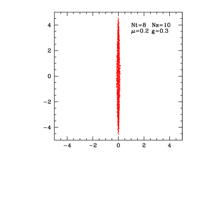
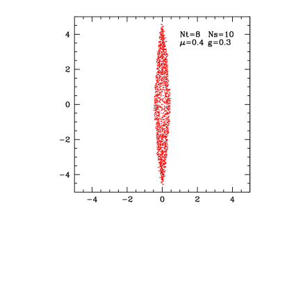
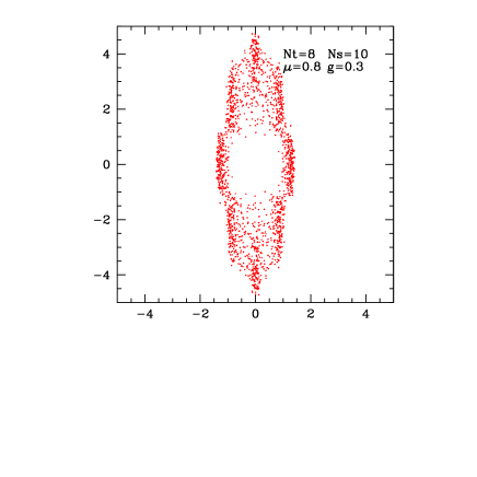
FIG. 8.: Eigenvalues in the mass plane for $N_{t}=8$, $N_{s}=10$, $g=0.3$, $\mu=0.20$, $0.40$, and $0.80$ respectively, from left to right. The initial line of eigenvalues along the imaginary axis widens in the real direction. For combinations of large $\mu$ and small $g$ the eigenvalues are grouped around $N_{t}$ points located symmetrically inside the ellipsoidal cloud.

The eigenvalues corresponding to the $\mu$ dependence are perhaps more interesting from a practical point of view. The natural variable is the fugacity $\xi=e^{\mu}$. We are interested in eigenvalues in the complex fugacity plane, corresponding more closely to the ones calculated in the Glasgow method [6] in lattice simulations. We seek the complex values of the fugacity which cancel the fermion determinant $D+m$ for a given random matrix ’configuration’ $C$. We apply Gibbs’ trick [9] to construct a matrix whose eigenvalues are explicitly the zeros in the fugacity plane. Let us define the matrices

$$G~{} = ~{}\left(\begin{array}[]{cc}m&iC\\ iC^{\dagger}&m\end{array}\right)$$ (24)

$$V~{} = ~{}\left(\begin{array}[]{cc}0&\hbox{\zfont S \kern-7.5ptS}_{N_{t}}\\ \hbox{\zfont S \kern-7.5ptS}_{N_{t}}&0\end{array}\right)$$ (27)

$$\bar{V}~{} = ~{}\left(\begin{array}[]{cc}0&\hbox{\zfont S \kern-7.5ptS}_{N_{t}}^{T}\\ \hbox{\zfont S \kern-7.5ptS}_{N_{t}}^{T}&0\end{array}\right)~{}~{}.$$ (30)

so that the fermion matrix is written $D+m=G+\xi V-\xi^{-}1\bar{V}$. It is straightforward to check that

$$\det(D+m)~{}=~{}\det\left(\xi^{-1}V\right)\det\left(\begin{array}[]{cc}G\bar{V}+\xi\otimes\hbox{\zfont 1 \kern-6.99997pt1}_{N}&\bar{V}\\ \bar{V}&\xi\otimes\hbox{\zfont 1 \kern-6.99997pt1}_{N}\end{array}\right)~{}~{}.$$ (33)

where we again used the formula for reducing the size of the determinant by $2$. Hence we are interested in the eigenvalues of the propagator matrix

$$F(m)~{}=~{}\left(\begin{array}[]{cc}G\bar{V}&\bar{V}\\ \bar{V}&0\end{array}\right)~{}=~{}\left(\begin{array}[]{cc}G&\hbox{\zfont 1 \kern-6.99997pt1}_{N_{t}}\\ \hbox{\zfont 1 \kern-6.99997pt1}_{N_{t}}&0\end{array}\right)\left(\begin{array}[]{cc}\bar{V}&0\\ 0&\bar{V}\end{array}\right).$$ (40)

If the size $g$ of the random matrix is small, the $\xi$-eigenvalues are just the $N_{t}$ order roots of unity. As $g$ increases, they are located in a cloud around those values. The size of the cloud increases with $g$, to the point where the eigenvalues merge into a ring around zero. In figure 9 we plot only the eigenvalues larger than $1$ in absolute value (since if $\xi$ is an eigenvalue, so is $1/\xi$).

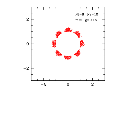
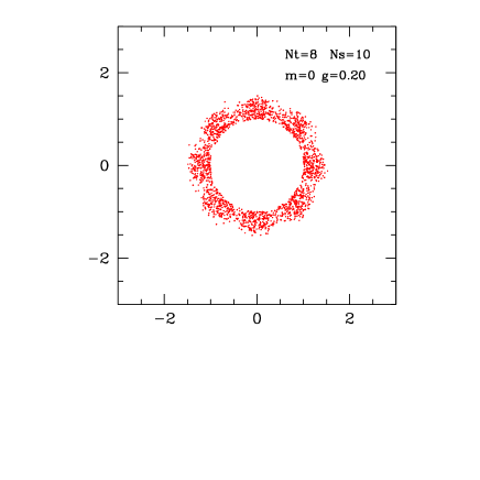
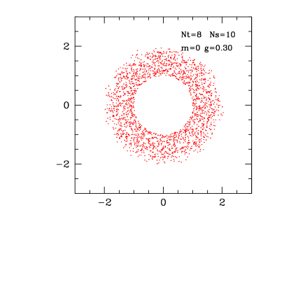
FIG. 9.: Eigenvalues in $\xi_{k}$ the fugacity plane for $N_{t}=8$, $N_{s}=10$, $m=0$ and $g=0.15$, $0.20$, and $0.30$ respectively, from left to right. Only the ones with $|\xi_{k}|\leq 1$ are plotted. For small $g$ the eigenvalues are concentrated around the roots of unity and merge into a circular band as $g$ increases.

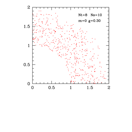
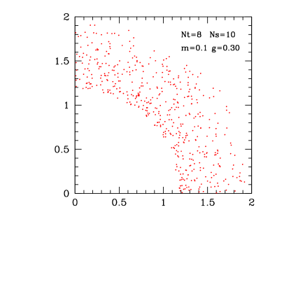
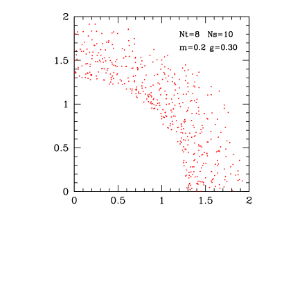
FIG. 10.: Eigenvalues in the fugacity plane for $N_{t}=8$, $N_{s}=10$, $g=0.30$ and $m=0.0$, $0.1$, and $0.2$ respectively, from left to right. Only the ones with $|\xi_{k}|\leq 1$ are plotted. There is gap around $1$ which increases with $m$.

B Partition function zeros

The zeros of the partition function in exactly solvable models provide an interesting link between finite size and continuum properties. In the present case one can easily calculate them by expanding (6) in powers of $e^{\mu}$ or $m$.

It is a well known phenomenon which we have also discussed in some technical detail in [7], that the zeros trace out the analytic continuation of the phase boundaries into the complex plane of the respective model parameter.

This is illustrated in Figure 11, where we show the partition function zeros in the fugacity plane at zero mass, for the same $N_{s}=10$ and two different $N_{t}$ values, $8$ and $40$. The smaller value corresponds to Glasgow simulations [6], where they used eight timeslices. Notice that the zeros are significantly away from a circle, which would be the continuum result. In the same figures we plot the analytical line corresponding to the transition in the complex fugacity plane, for the same $N_{t}$ values, but using the saddle point approximation in $N_{s}$.

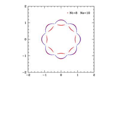
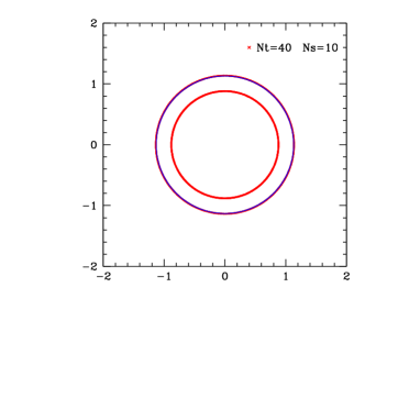
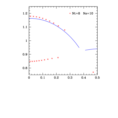
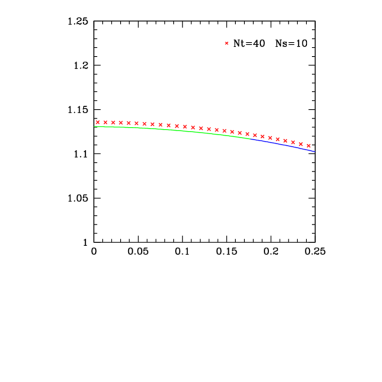
FIG. 11.: Partition function zeros and the analytical curve that separates the two saddle points in the complex $\mu$ plane. The curve within the unit circle is just the ’mirror image’ of the one outside, since everything is symmetric under $\mu\rightarrow 1/\mu$. In the limits of large $N_{t}$, the curves become circles at $|\mu|=\mu_{c}$ and $1/\mu_{c}$ . The partition function zeros trace out nicely the saddle point result, even for a moderate $N_{s}=10$.

In Figures 12 and 13 we plot partition function zeros for $N_{t}=8$ and various values of the quark mass $m$ and the size parameter $g$. As the mass is increased, the two lines of zeros move away from the unit circle. For small values of the size parameter $g$, the zeros sit in loops around the $N_{t}$ order complex roots of unity.

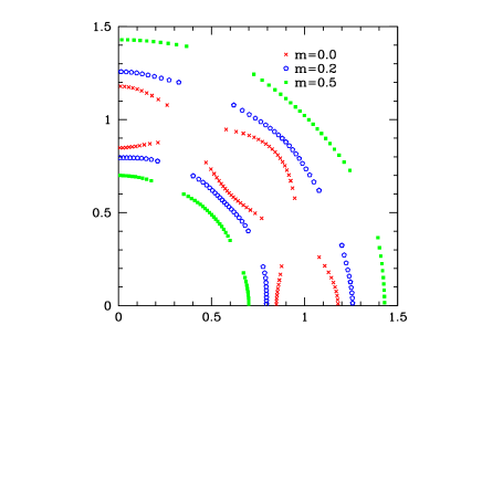
FIG. 12.: Partition function zeros in the complex fugacity plane, for $N_{t}=8$ and $N_{s}=10$, for various mass values.

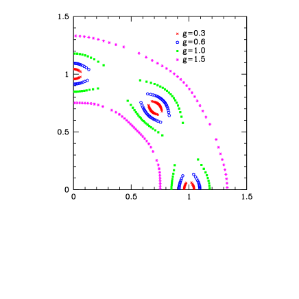
FIG. 13.: Partition function zeros in the complex fugacity plane, for $N_{t}=8$ and $N_{s}=10$, for various values of the size parameter $g$.

V Conclusions

We have constructed a random matrix model for the chiral phase transition at finite chemical potential with a $\mu$ dependence more similar to that in the lattice implementation of the problem. Our approach may be interpreted as ensuring time translation invariance in the large $N_{t}$ limit. We analyzed the model in the saddle point approximation with respect to the number $N_{s}$ of points per timeslice (or number of instanton modes). Similarly to the usual RMM, our model features a first-order phase transition driven by the chemical potential $\mu$. Both the particle number $\langle n\rangle$ and the chiral condensate have a finite jump at this transition. The finite jump, hence the first order character, survive when the quark mass is increased.

We calculated the eigenvalues of the Dirac operator in both the complex quark mass plane and the complex plane of the fugacity, $e^{\mu}$. The distributions of the eigenvalues show a strong qualitative similarity to those encountered in lattice simulations. We also calculated the zeros of the partition function in the fugacity plane for various parameter values and found that their location is well approximated by the phase transition curve obtained from the saddle point analysis of the effective partition function.

The most remarkable property of the model is the $\mu$-independence of the partition function in the low density phase, when the number of timeslices $N_{t}$ is large. As a consequence, the number density is identically zero in this phase. This property is different from what is seen in the traditional RMM [4, 5], where there was a negative number density in the low density phase, which coincided with a suppression of the partition function. Our previous conclusion on the mechanism that made the Glasgow method exponentially slow points precisely towards this suppression as the ultimate source of trouble [7].

For small $N_{t}$ values the suppression of the partition function is significant in this model, too. However, it disappears quickly as $N_{t}$ increases, together with the $\mu$ dependence in the broken phase, as one would expect in continuum QCD. The Glasgow lattice simulations which have been reported [6] employed a small number of timeslices, corresponding to $N_{t}=8$, $N_{t}^{\prime}=4$ in our model. For this value, we find a significant suppression of the partition function. The suppression is further enhanced by the number of spatial points, corresponding to our $N_{s}$, which is of order $N_{t}^{3}$ in a traditional lattice simulation. This leads to the exciting possibility that lattice (Glasgow) simulations of QCD at finite $\mu$ might be plagued by the same problem of a spuriously suppressed partition function, as one finds in the RMM. The suppression is an artifact of time discretization, and could in principle be cured by using a large number of timeslices and a small spatial lattice.

The main argument against excessive enthusiasm is the fact that in the present model, similarly to the usual RMM, we have a major cancellation due to averaging. Averaging over the phases of the determinant achieves a cancellation in the broken or low density phase, namely from the magnitude of the typical determinant, of the order of $\exp(2\mu N)$, a large number, to that of the same determinant at $\mu=0$, which is of the order $1$. This cancellation appears then to be similar to the one seen in the usual RMM. However, in that case the determinant at $\mu\neq 0$ was not significantly larger than $1$, and the cancellation due to phase averaging led to a small number, $\exp(-\mu^{2}N)$. That cancellation coincides with the suppression of the partition function at $\mu\neq 0$ with respect to its value at $\mu=0$. As we have learned from the analysis of the Glasgow method applied to that model, a partition function which is suppressed for some parameter values is very hard to calculate because of the huge precision required.

One should make a distinction between the cancellation brought about by phase averaging, i.e., from $<|det(\mu)|>$ to $<det(\mu)>$, and the suppression of the partition function, i.e., from $<det(0)>$ to $<det(\mu)>$. A partition function like the present one, which is the result of large cancellations during averaging, but does not have significant suppression, in not a priori incalculable from simulations, and might be amenable to a calculable form using an appropriate resummation [13].

Our previous study of Glasgow averaging [7] in the usual RMM indicates the suppression of the partition function, $Z(\mu)/Z(0)<<1$ as the source of trouble. The pattern of false zeros was not driven by the competition between the true partition function and the Stephanov phase (defined by the absolute value of the determinant), but rather between the former and a phase resulting from spoiling the cancellation between various terms of the polynomial expansion of the true partition function. It is probably too early at this point to encourage a new set of lattice Glasgow simulations. However, a reexamination of the Glasgow method in the context of this model might lead to encouraging results.

Our model is similar to those arising from strong-coupling analysis of lattice QCD at finite $\mu$ [10], but it has the simplicity of random matrix models. There is a straightforward connection with RMM models with many Matsubara frequencies [11]. This can be seen by diagonalizing the hopping matrix in the original form of the partition function. Extracting a $T-\mu$ phase diagram from this model is also possible. Introducing a dimensionful lattice spacing $a$ leads to identifying the quantity $aN_{t}$ with the inverse temperature. However, a more careful analysis of the implementation of temperature in this model should precede that.

In summary, we studied a simple model which shows a clear connection between time translation invariance and the physical requirement of having a zero baryon number density in the low density phase of QCD. The careful implementation of time dependence seems to have the potential to cure one of the artifacts that make traditional lattice simulations at finite density virtually impossible.

It would be interesting to see how the introduction of an explicit temperature dependence in this model would change the $\mu-T$ phase diagram that emerges from the usual random matrix model. Also, it would be very interesting to see how the exciting results obtained in the RMM for color superconductivity [12] would be influenced by our method of introducing the chemical potential.

This work has been supported in part by a grant from the U.S. National Science Foundation. Thanks are due to James Osborn, Dirk Rischke, Dominique Toublan, and Jac Verbaarschot for many useful discussions. Ralph Amado, Dirk Rischke and Jac Verbaarschot are thanked for a critical reading of the manuscript. I am grateful to the Nuclear Theory Group at BNL for their hospitality during part of the time the paper was written.

A Derivation of $\det\left(Q_{N}(a,x)\right)$

We wish to study matrices of the form

$${\cal Q}_{L}(a,x)~{}=~{}\left(\begin{array}[]{cccc}a&x&\cdots&x^{-1}\\ x^{-1}&\ddots&\ddots&\vdots\\ \vdots&\ddots&\ddots&x\\ x&\cdots&x^{-1}&a\end{array}\right)~{}~{}=~{}~{}a\otimes\hbox{\zfont 1 \kern-6.99997pt1}_{N}+x\otimes\hbox{\zfont S \kern-7.5ptS}_{N}+x^{-1}\otimes\hbox{\zfont S \kern-7.5ptS}_{N}^{T}.$$ (A5)

which occur in the dual representation of our partition function. This result can also be found in [14]. We derive it here for completeness. The size of the matrix $N$ is an arbitrary positive integer. There are no special restrictions on $a$ and $x$. This determinant is We will calculate the determinant by induction. First, we define an auxiliary matrix,

$$\tilde{\cal Q}_{N}(a,x)~{}=~{}\left(\begin{array}[]{cccc}a&x&\cdots&0\\ x^{-1}&\ddots&\ddots&\vdots\\ \vdots&\ddots&\ddots&x\\ 0&\cdots&x^{-1}&a\end{array}\right)~{}~{}.$$ (A10)

The respective determinants $Q_{N}$ and $\tilde{Q}_{N}$ verify

$$Q_{N}~{}=~{}a\tilde{Q}_{N-1}-2\tilde{Q}_{N-2}-(-)^{N}\left(x^{N}+\frac{1}{x^{N}}\right)~{}~{},$$ (A11)

which is obtained as follows. First expand $Q_{N}$ by its first row, which leads to three sub-determinants, one of them $\tilde{Q}_{N-1}$. Expand again the remaining two by their first column, which leads to two matrices $\tilde{Q}_{N-2}$ and triangular matrices, which give the $x^{\pm N}$ terms. The same trick applied to $\tilde{Q}_{N}$ yields a recursion relation,

$$\tilde{Q}_{N}~{}=~{}a\tilde{Q}_{N-1}-\tilde{Q}{{}_{N}-2}~{}~{}.$$ (A12)

We have $\tilde{Q}_{2}=a^{2}-1$ and $\tilde{Q}_{3}=a^{3}-2a$, which leads to $\tilde{Q}_{0}=1$ and $\tilde{Q}_{1}=a$. The recursion formula (A12) can be solved explicitly. First, notice that the recursion is homogeneous so if two distinct series $\left\{q_{k}\right\}$ and $\left\{q^{\prime}_{k}\right\}$ verify the recursion relation, so will any linear combination of the two series. Of course, there may be at most two linearly independent solutions, since the first two terms of a given solution completely define the whole solution. We seek the solution in the form of a power series, $q_{k}=A\xi^{k}$. The base $\xi$ must then verify the characteristic equation

$$\xi^{2}-a\xi+1=0~{}~{}.$$ (A13)

Consider the two roots of (A13), $\lambda_{12}(a)=\frac{1}{2}\left(a\pm\sqrt{a^{2}-4}\right)$. They are each others’ inverse, $\lambda_{1}(a)=\frac{1}{\lambda_{2}(a)}$, and their sum is $a$. We can then write $\tilde{Q}_{k}=\alpha_{1}\lambda_{1}^{k}+\alpha_{2}\lambda_{2}^{k}$, where the coefficient-a $\alpha_{12}$ are determined from the first two terms in the series, as

$$\alpha_{1}~{}=~{}\frac{\lambda_{1}}{\lambda_{1}-\lambda_{2}}~{}~{};~{}~{}\alpha_{2}~{}=~{}\frac{-\lambda_{2}}{\lambda_{1}-\lambda_{2}}~{}~{}.$$ (A14)

The result $\tilde{Q}_{N}=\frac{\lambda_{1}^{N+1}-\lambda_{2}^{N+1}}{\lambda_{1}-\lambda_{2}}$ finally leads to the following expression for the original determinant:

$$Q_{N}~{}=~{}\lambda^{N}+\lambda^{-N}-(-)^{N}\left(x^{N}+x^{-N}\right)~{}~{}.$$ (A15)

where for simplicity we defined $\lambda\equiv\lambda_{1}=\frac{1}{2}\left(a\pm\sqrt{a^{2}-4}\right)=\frac{1}{\lambda_{2}}$.

REFERENCES

- [1] M.A. Stephanov, Phys. Rev. Lett. 76 (1996) 4472; Nucl. Phys. Proc. Suppl. 53 (1997) 469.
- [2] J. Kogut, H. Matsuoka, M. Stone, H.W. Wyld, Nucl. Phys. B225 (1983) 93.
-
[3]
J.B. Kogut, M.P. Lombardo, D.K. Sinclair,
Phys. Rev. D51 (1995) 1282.
M.P. Lombardo, J.B. Kogut, D.K. Sinclair, Phys. Rev. D54 (1996) 2303. - [4] M.Á. Halász, A.D. Jackson, R.S. Shrock, M.A. Stephanov, J.J.M. Verbaarschot, Phys. Rev. D58 (1998) 096007.
- [5] M.Á. Halász, A.D. Jackson, J.J.M. Verbaarschot, Phys. Rev. D56 (1997) 5140.
-
[6]
I.M. Barbour, S.E. Morrison, E.G. Klepfish, J.B. Kogut, M.P. Lombardo,
Phys. Rev. D56 (1997) 7063.
I.M. Barbour, Nucl. Phys. A642, (1998) 251c. -
[7]
M. A. Halasz, Nucl.Phys. A642 (1998) 342c.
M. A. Halasz, J. C. Osborn, M. A. Stephanov and J. J. Verbaarschot, Phys. Rev. D61, 076005 (2000) -
[8]
H. Markum, R. Pullirsch, T. Wettig, Phys.Rev.Lett. 83 (1999) 484;
B.A. Berg, H. Markum, R. Pullirsch, T. Wettig, hep-lat/9912055. M.P. Lombardo, hep-lat/9908066 - [9] P.E. Gibbs, Phys. Lett. B172 (1986) 53.
- [10] N. Bilic, K. Demeterfi, B. Petersson, Nucl. Phys. B 377 (1992) 651.
-
[11]
R. A. Janik, M. A. Nowak, G. Papp and I. Zahed,
Nucl. Phys. A642, 191 (1998)
R.A. Janik, M.A. Nowak and I. Zahed , Phys. Lett. B392 (1997) 155.
T. Wettig, in Proceedings of “Hirschegg ’97: QCD phase transitions”, eds. H. Feldmeier, J. Knoll, W. Noerenberg, and J. Wambach, p. 69 (GSI, Darmstadt, 1997);
T. Wettig, T. Guhr, A. Sch fer, H. A. Weidenm ller, hep-ph/9701387 -
[12]
B. Vanderheyden and A. D. Jackson,
Phys. Rev. D62, 094010 (2000),
B. Vanderheyden and A. D. Jackson, Phys. Rev. D61, 076004 (2000) - [13] S. Chandrasekharan, U.J. Wiese, Phys.Rev.Lett. 83 (1999) 3116.
- [14] P.E. Gibbs, Phys.Let.. B182 (1986) 369.