Study of Charmonia near the deconfining transition on an anisotropic lattice with O(a) improved quark action

Abstract

We study hadron properties near the deconfining transition in the quenched lattice QCD simulation. This paper focuses on the heavy quarkonium states, such as $J/\psi$ meson. In order to treat heavy quarks at $T>0$, we adopt the $O(a)$ improved Wilson action on anisotropic lattice. We discuss $c\bar{c}$ bound state observing the wave function and compare the meson correlators at above and below $T_{c}$. Although we find a large change of correlator near the $T_{c}$, the strong spatial correlation which is almost the same as confinement phase survives even $T\sim 1.5T_{c}$.

1 Introduction

It is generally believed that the Quantum Choromodynamics (QCD) exhibits a phase transition at some temperature $T_{c}$, and quarks and gluons confined in the low temperature phase are liberated to form the “quark gluon plasma”. At the beginning of 2000, CERN reported that the QGP state had been created in the heavy ion collision experiment[1]. In these experiments, the $J/\psi$ suppression[2] is regarded as the key signal of QGP formation. Since c-quark is heavy ( $m_{c}=1.15\sim 1.35$ GeV[3]) $c\bar{c}$ pair are hard to be generated except by the primary collisions of nucleons in the high energy heavy ion, i.e. the $J/\psi$ is not created with the thermal effects after the QGP formation. Therefor it is expected that the effects of deconfining clearly appear in this signal. Further investigation will be performed in RHIC project at BNL.

On the theoretical side, in spite of the various approaches[4, 5, 6], we are still far from the definite understanding of hadron properties near the transition and the fate of the hadronic states in the plasma phase. Since the phase transition changes the relevant degree of freedom of the system, the model approach which a priori assumes dynamical degrees of the system is difficult to treat physics near the phase transition. We investigate these problems using lattice QCD, which enables us to incorporate the nonperturbative effect of QCD from the first principle.

For a long time, in the lattice QCD simulations, hadron masses at finite temperature have been argued with the spatial correlation (screening mass)[7]. On the other hand, the study of the temporal correlation, which is related to the pole mass, has been started rather recently[8].

The previous work[8] studied hadron properties near the $T_{c}$ based on light quarks. They caught a sign of chiral symmetry restoration above $T_{c}$, and a change of correlators in temporal and spatial direction near the $T_{c}$. From the discussion of wave function, however, they find the same strong spatial correlation at $T>T_{c}$ as that of below $T_{c}$, in other words hadronic mode at a long range survives in the deconfinement phase. At present, there is no well-established way of lattice simulations to attack the spectroscopy at $T>0$. However, our recent work seems one of the best approaches to the problem. It is interesting to apply this analysis to the heavy quarks. In this paper we focus on the heavy quarkonium state, which plays an important role as a signal of the quark gluon plasma formation[2, 9].

Our goal of the investigation is the prediction about $J/\psi$ suppression or mass shift of charmonium[9] as signals of QGP formation and the understanding of hadron properties and nature of QGP phase near the transition.

For the study of charmonium physics at $T>0$ on a lattice, there are several problems. Then we classify these problems into two category, and discuss them individually.

(i)

Precise calculation of temporal correlator of charmonium at $T>0$

(ii)

Extraction of physical properties of charmonium from the correlators

Firstly we consider the former one. In the lattice QCD simulation at $T>0$, we set a temporal lattice extent to $1/T$. At high temperature, one needs the large lattice cutoff to work with the sufficient degrees of freedom in the temporal direction. In order to obtain the detailed information of temporal meson correlators at $T>0$, a high resolution in temporal direction is needed. The large lattice cutoff is also necessary to study a correlator of meson with the heavy quarks because of its rapid decreasing behavior. If one tries to overcome these difficulties with straightforward way, the tremendous large computational power is necessary. In order to get the sufficiently fine resolution with limited computer resources, we use the anisotropic lattice, which has a finer temporal lattice spacing $a_{\tau}$ than the spatial one $a_{\sigma}$.

In this work we adopt the same strategy as the previous work[8] which was tractable to analyze light hadrons at $T>0$. This strategy is as follows. Firstly the mesonic operator are defined, then we observe its correlator and wave function (in the Coulomb gauge) at $T=0$. Next we investigate how they are affected by the temperature. In order to investigate the temperature effects for the state of interest, for example a ground and excited state of charmonium, we have to make the good mesonic operator which has the large overlap with the state. Because we should compare correlators at $T\geq 0$ within shorter temporal lattice extent. The wave function gives hints for existence of mesonic state at $T>0$. Especially we are interested in that of deconfinement phase. In the case of charmonium this wave function is an important quantity concerning the $J/\psi$ suppression.

We prepare two sets of gauge configuration whose lattice spacing are different. We control the temperature by changing temporal lattice extent $N_{t}$. Then above investigation is performed on these configurations.

This paper is organized as follows. In the next section we define the quark action on anisotropic lattice and discuss the dispersion relation of free quark and calibration of quark field. Sect. 3 is the preparation for study of charmonium correlator. Here various parameters of gauge configurations are determined and the calibration are performed. In Sect. 4 we report the charmonium spectroscopy and construction of optimized operator using variational analysis at $T=0$. Sect. 5 describes correlators at $T>0$ and the measurement of the wave function and compare these with results at $T=0$. The last section is the conclusion and discussion.

2 Quark action on the anisotropic lattice

2.1 Quark action

To treat the quark field on the lattice, we adopt the $O(a)$ improved Wilson quark formulation. To construct the quark action on the anisotropic lattice, we follow El-Khadra, Kronfeld and Mackenzie[10], for the following advantages. They expand the lattice Hamiltonian in the power of $a$, and determine the coefficient of each operator by matching the lattice Hamiltonian with the the continuum one except the redundant operators. The resultant action takes the same form as the clover quark action[11] in the limit of $m\rightarrow 0$. On the other hand, in the heavy quark mass region ($m_{q}\gg\Lambda_{QCD}$), the effective-theoretical treatment of the quark action enables us to use it for such a quark on a lattice of moderate cutoff. Since the full quark mass dependence is incorporated, the same form also covers the intermediate quark mass region, and then the small and the large mass regions are smoothly connected. Although our main target in this paper is the charm quark, it would be useful to take the other mass region into account for the future applications. In addition to these advantages, their argument is naturally in accord with the anisotropic lattice. They introduced the different hopping parameters for the spatial and the temporal directions, and proposed to tune them so that the rest and the kinetic mass take the same value. Such a treatment is inevitably required on the anisotropic lattice to assure that the anisotropy of the quark and the gauge fields coincide, especially if one employ the dispersion relation for the definition of the quark field anisotropy.

On the anisotropic lattice, the quark action takes almost the same form as in the Ref. [10] :

$$S_{F}=\sum_{x,y}\bar{\psi}(x)K(x,y)\psi(y),$$ (1)

$$K(x,y) = \delta_{x,y}-\kappa_{\tau}\left\{(1-\gamma_{4})U_{4}(x)\delta_{x+\hat{4},y}+(1+\gamma_{4})U_{4}^{{\dagger}}(x-\hat{4})\delta_{x-\hat{4},y}\right\}$$ (2)

$$\hskip 19.91684pt-\kappa_{\sigma}\sum_{i}\left\{(r-\gamma_{i})U_{i}(x)\delta_{x+\hat{i},y}+(r+\gamma_{i})U_{i}^{{\dagger}}(x-\hat{i})\delta_{x-\hat{i},y}\right\}$$

$$\hskip 19.91684pt-\kappa_{\sigma}c_{E}\sum{i}\sigma_{4i}F_{4i}(x)\delta_{x,y}-r\kappa_{\sigma}c_{B}\sum_{ij}\frac{1}{2}\sigma_{ij}F_{ij}(x)\delta_{x,y}.$$

The spatial and the temporal hopping parameters, $\kappa_{\sigma}$ and $\kappa_{\tau}$ respectively, are related to the bare quark mass $m_{0}$ and the bare anisotropy parameter $\gamma_{F}$ as follows.

$$\kappa_{\sigma} = \frac{1}{2(m_{0}+\gamma_{F}+3r)},$$ (3)

$$\kappa_{\tau} = \gamma_{F}\kappa_{\sigma}.$$ (4)

where the $m_{0}$ is in the spatial lattice unit. In the free quark case, the bare anisotropy $\gamma_{F}$ is taken to be the same value as the cutoff anisotropy $\xi=a_{\sigma}/a_{\tau}$. In practical simulation, the anisotropy parameter receives the quantum effect and should be tuned to give the same renormalized anisotropy for the fermion and the gauge fields. This “calibration” will be described later.

There have been used two choices of the value of the Wilson parameter $r$ for the anisotropic $O(a)$ improved quark action. In this work, we adopt the choice[8] $r=1/\xi$. In this case, the temporal and the spatial directions are treated in the equal manner in the physical unit. As the result, the tree level dispersion relation holds the axis-interchange symmetry in the lowest order of $\vec{p}^{2}$. On the other hand, this choice decreases the masses of doublers which are introduced by the Wilson term to eliminate the unwanted poles at the edges of the Brillouin zone. The dispersion relation is examined in the later part of this section. Alternative choice, $r=1$, are adopted in the Ref. [12, 13, 14]. In this case, the contribution of doublers would not cause any problem, in the cost of manifest axis-interchange symmetry. Since we aim to develop the form applicable to the whole quark mass region, $r=1/\xi^{-1}$ seems preferable especially in the light quark mass region.

Here it is useful to define $\kappa$ so that which has the same relation with the bare quark mass $m_{0}$ as the isotropic case:

$$\frac{1}{\kappa}=\frac{1}{\kappa_{\sigma}}-2(\gamma_{F}+3r-4)\hskip 14.22636pt(\,=2(m_{0}+4)\,).$$ (5)

For the light quark systems, the extrapolation to the chiral limit would be performed in $1/\kappa$. The coefficients of the clover terms, $c_{E}$ and $c_{B}$, depend on the Wilson parameter $r$. In our choice $r=\xi^{-1}$, $c_{E}$ and $c_{B}$ are unity at the tree level.

We apply the mean-field improvement proposed in the Ref. [15]. On the anisotropic lattice, the mean-filed values of the spatial link variable $u_{\sigma}$ and the temporal one $u_{\tau}$ are different from each other. The improvement is achieved by rescaling the link variable as $U_{i}(x)\rightarrow U_{i}(x)/u_{\sigma}$ and $U_{4}(x)\rightarrow U_{4}(x)/u_{\tau}$. This replacement leads the following values for the coefficient of the clover terms.

$$c_{E}=\frac{1}{u_{\sigma}u_{\tau}^{2}},~{}~{}~{}c_{B}=\frac{1}{u_{\sigma}^{3}}.$$ (6)

The determination of mean-field values of the link variable $u_{\sigma}$ and $u_{\tau}$ are described in the next section.

In this paper, our target mass region is around the charm quark mass. The temporal cutoffs in this work are $4.5$ and $6.4$ GeV, and well above the charm quark mass. For these quark mass and $a_{\tau}^{-1}$, the effective-theoretical treatment would not be necessary to be applied. Such consideration will be called for the calculations containing the $b$-quark on the same size of lattice. In the effective-theoretical treatment, the ratio of the spatial and the temporal hopping parameter is tuned so that they give correct dispersion relation of the nonrelativistic quark[10]. On the anisotropic lattice, the calibration automatically incorporates this condition if one use the nonrelativistic dispersion relation as the anisotropy condition.

2.2 Dispersion relation of free quark

Now we consider how the dispersion relation of the free quark is changed by the introduction of anisotropy. Observing the action (2), one notices that the larger anisotropy $\xi$ causes the smaller spatial Wilson term. Then the question is how the contribution of the doubler eliminated by the Wilson term becomes significant. The action (2) leads the free quark propagator,

$$S(p)=\frac{1}{i\gamma_{4}\sin{p_{4}}+i\;\zeta\vec{\gamma}\cdot\vec{S}+m_{t}+(1-\cos p_{4})+\frac{1}{2}r\zeta\vec{\hat{p}}^{2}},$$ (7)

where $\zeta=\xi^{-1}$, $m_{t}=m_{0}\zeta$, $S_{i}=\sin p_{i}$ and $\hat{p_{i}}=2\sin(p_{i}/2)$. Then the dispersion relation of the free quark is

$$\cosh E(\vec{p})=1+\frac{\zeta^{2}\vec{S}^{2}+(m_{t}+\frac{1}{2}r\zeta\vec{\hat{p}}^{2})^{2}}{2(1+m_{t}+\frac{1}{2}r\zeta\vec{\hat{p}}^{2})}.$$ (8)

Neglecting the higher order terms in $\vec{p}$ and in $a$, the relativistic dispersion relation $E^{2}=m^{2}+\zeta^{2}\vec{p}^{2}$ holds for the small quark mass. ($m^{2}=m_{t}^{2}(1-m_{t})$, and $m_{t}$ is the bare parameter.)

Fig. 1 shows the dispersion relation (8) at $\xi=5.3$ and $4.0$ for various values of $m_{t}$. Now let us consider the practical cases that $a_{\tau}^{-1}=4.5$ GeV for $\xi=5.3$ (Set-I) and $a_{\tau}^{-1}=6.4$ GeV for $\xi=4.0$ (Set-II). These values are obtained in our numerical simulations, and described in the next section. In the heavy quarkonium, the typical energy and momentum exchanged inside the meson are in the order of $mv^{2}$ and $mv$ respectively[16]. For the charmonium, $v^{2}\sim 0.3$, then typical scale of the kinetic energy is around $500$ MeV. It is noted that $m_{t}\sim 0.3$ for Set-I and $m_{t}\sim 0.2$ for Set-II correspond to the charm quark mass. Let us consider two quarks inside meson with opposite momenta $p=\pm\pi/a$. Then $2(E(p_{z}=a/\pi)-E(0))\sim 0.5$ GeV and $\sim 1$ GeV for Set-I and Set-II respectively. Although Set-I lattice may not be free from the systematic effect, Set-II would be successfully applicable to the low-lying charmonium system.

For comparison, we also examine the light quark mass region. For Set-I, $m=0.02$–$0.06$ corresponds to 90-270 MeV, which is used in the Ref. [8] as the light quark mass region with the anisotropic Wilson quark action with $r=1$. $E(\vec{p})-E(0)$ rapidly decrease at the edge of the Brillouin zone, and the height at $z=a/\pi$ is around 300 MeV. For two quarks with momenta $p=\pm a/\pi$, additional energy of doublers is $\sim 600$ MeV, and again seems not sufficiently large compared with the typical energy scale transfered inside mesons. In the case of Set-II, this value increases to 1.4 GeV, and seems to be applicable to the meson systems without large systematic effect.

Figure 1: Dispersion relation of anisotropic free quark. Left figure is of Set-I, right one is of Set-II.

2.3 Calibration of quark field

On anisotropic lattice, the anisotropy of quark configuration $\xi_{F}$ must be equal to that of gauge field $\xi$.

$$\xi(\gamma_{G},\gamma_{F})=\xi_{F}(\gamma_{G},\gamma_{F})$$ (9)

Since $\xi$ and $\xi_{F}$ are function of $\gamma_{G}$ and $\gamma_{F}$ in general, a nonperturbative determination of the combination of $\gamma_{G}$ and $\gamma_{F}$ which satisfy the condition (9) requires much effort. In the quenched case, however, these determination are rather easy to be performed, because $\xi$ can be determined independently of $\gamma_{F}$. After the determination of $\xi$, one can tune $\gamma_{F}$ so that the certain observable satisfies the condition (9). We call this procedure as “calibration”.

There are several determinations of $\xi_{F}$. In the Ref. [8], the ratio of the temporal to the spatial meson masses, $\xi_{F}=m_{\sigma}/m_{\tau}$, is used as such a observable. However this is not suitable for the present case, since the charm quark mass is larger than or comparable with the spatial lattice cutoffs. In order to determine $\xi_{F}$, we use the dispersion relation of the free meson[12, 13, 14]. For a heavy quark, one may use the nonrelativistic dispersion relation, $E=m+p^{2}/2m\xi_{F}^{2}$. In this paper, we alternatively use the relativistic dispersion relation of meson for the calibration. This form is also available for the light quark mass region.

We assume that the meson is described by the following lattice Klein-Gordon action.

$$S=\sum_{x}\frac{1}{2\xi_{F}}\phi^{{\dagger}}(x)\left[-\xi_{F}^{2}D_{4}^{\,2}-\vec{D}^{2}+m_{0}^{2}\right]\phi(x),$$ (10)

where $m_{0}$ is in the unit of $a_{\sigma}$. Then the free meson satisfies the dispersion relation

$$\cosh E(\vec{p})=1+\frac{1}{2\xi_{F}^{2}}(\vec{\hat{p}}^{2}+m_{0}^{2}).$$ (11)

Using this relation, one can determine the anisotropy $\xi_{F}$ as

$$\xi_{F}^{2}=\frac{\vec{\hat{p}}^{2}}{2(\cosh E(\vec{p})-\cosh E(0))}$$ (12)

This condition forces the axis-interchange symmetry to the meson field.

3 Lattice setup

3.1 Gauge configuration

The numerical calculations performed on the two sets of anisotropic lattices[17], one is with the standard plaquette action and the other is with Symanzik type improved action at the tree level[18]. These actions are represented with the following form;

$$S_{G} = \frac{\beta}{\gamma_{G}}\sum_{x,i<j\leq 3}\left[c_{11}(1-P_{ij}(x))+c_{12}(2-R_{ij}(x)-R_{ji}(x))\right]$$ (13)

$$+\beta\gamma_{G}\sum_{x,i\leq 3}\left[c_{11}(1-P_{i4}(x))+c_{12}(2-R_{i4}(x)-R_{4i}(x))\right],$$

where the plaquette $P_{\mu\nu}(x)$ and rectangular loop $R_{\mu\nu}(x)$ are defined as follows,

$$P_{\mu\nu}\equiv\frac{1}{3}\mbox{Re}\mbox{Tr}[U_{\mu}(x)U_{\nu}(x+\hat{\mu})U^{\dagger}_{\mu}(x+\hat{\nu})U^{\dagger}_{\nu}(x)]$$ (14)

$$R_{\mu\nu}\equiv\frac{1}{3}\mbox{Re}\mbox{Tr}[U_{\mu}(x)U_{\mu}(x+\hat{\mu})U_{\nu}(x+2\hat{\mu})U^{\dagger}_{\mu}(x+\hat{\nu}+\hat{\mu})U^{\dagger}_{\mu}(x+\hat{\nu})U^{\dagger}_{\nu}(x)].$$ (15)

The standard action is the case with $c_{11}=1$ and $c_{12}=0$, and the improved action is $c_{11}=5/3$ and $c_{12}=-1/12$. The Set-I is the same configurations as used in the Ref. [8]. The parameters for these configurations are summarized in Table 1. These parameters are adopted so that the spatial and temporal lattice extent are about 3 fm respectively.

Both numerical calculations are done on the quenched configurations which are generated by the pseudo-heat bath algorithm with 20,000 thermalization sweeps, the configurations being separated by 2,000 sweeps. These configurations are fixed to Coulomb gauge. The statistical errors are estimated using the jackknife method unless mentioned explicitly.

Set	$c_{11}$	$c_{12}$	size	$\beta$	$\gamma_{G}$	# conf.
Set-I	1	0	$12^{3}\times N_{t}$	5.68	4.00	60
Set-II	5/3	-1/12	$16^{2}\times 24\times N_{t}$	4.56	3.45	120

Table 1: Simulation parameters for the gauge configurations.

We determine the parameters for the gauge field configurations, renormalized anisotropy $\xi(\equiv a_{\sigma}/a_{\tau})$ and spatial cutoff scale $a^{-1}_{\sigma}$. We define the ratios of the Wilson loop on spatial-spatial ($\sigma\sigma$) and spatial-temporal ($\sigma\tau$) plane[19, 20, 21].

$$R_{\sigma}(r,x) = W_{\sigma\sigma}(r,x)/W_{\sigma\sigma}(r+1,x),$$ (16)

$$R_{\tau}(r,t) = W_{\sigma\tau}(r,t)/W_{\sigma\tau}(r+1,t)$$ (17)

Then $\xi$ is determined so that the matching condition, $R_{\sigma}(r,x)=R_{\tau}(r,t=\xi x)$, is satisfied. From this analysis we conclude $\xi=5.3(1)$ (Set-I) and $\xi=3.950(18)$ (Set-II). Cutoff scales are determined from the static quark potential using the physical value of string tension $\sqrt{\sigma_{\mbox{\tiny phys}}}=427\mbox{MeV}$[22]. The spatial cutoff scales are $a_{\sigma}^{-1}=0.85(3)$ GeV (Set-I) and $1.610(14)$ GeV (Set-II) respectively.

From the calculation of Polyakov loops and its susceptibilities, we find that the temperatures of lattices with $N_{t}=18$ (Set-I) and $24$ (Set-II) are both just above $T_{c}$. Then we estimate $T_{c}=250\sim 260$ MeV from the temporal cutoff scale on our lattices. These estimation are consistent with the other quenched lattice results. We prepare the finite temperature gauge configurations at just below $T_{c}$, just above $T_{c}$ and about $1.5T_{c}$ for each sets. These results are summarized in Table 2.

Set	$\xi$	$a_{\sigma}^{-1}$(GeV)	$a_{\tau}^{-1}$(GeV)	$N_{t}(T/T_{c})$
Set-I	5.3(1)	0.85(3)	4.5(2)	72 ($\sim$ 0), 20 (0.93), 16 (1.15), 12 (1.5)
Set-II	3.950(18)	1.610(14)	6.359(62)	96 ($\sim$ 0), 26 (0.93), 22 (1.10), 16 (1.52)

Table 2: Scale parameters for the gauge configuration. The $\xi_{F}$, $a_{\sigma}^{-1}$ and $a_{\tau}^{-1}$ are measured on the configurations at $T=0$ ( $N_{t}=72~{}(\mbox{Set-I}),~{}96~{}(\mbox{Set-II})$). Here the temperatures are roughly estimated in the unit of $T_{c}$.

Here we notice that the hadronic correlator depends on which the sector Polyakov loop stays in $Z_{3}$ space at $T>T_{c}$. Since we treat the quenched QCD as an approximation of the full QCD, we choose the real sector for the value of Polyakov loop at $T>T_{c}$.

3.2 Mean-field value on the anisotropic lattice

We state the calculation of mean-filed value on the anisotropic lattice for the mean-field improvement of the clover coefficients.

There are two commonly used methods. One is determined from the expectation value of plaquette. This is widely used for its easiness to measure. On anisotropic lattice these are determined as follows.

$$u_{\sigma}=\frac{1}{3}\langle\mbox{Re}\mbox{Tr}P_{ij}(x)\rangle^{\frac{1}{4}},~{}~{}u_{\tau}=\frac{1}{3u_{\sigma}}\langle\mbox{Re}\mbox{Tr}P_{i4}(x)\rangle^{\frac{1}{2}}$$ (18)

The other is the trace of link calculated in the Landau gauge.

$$u_{\sigma}=\frac{1}{3}\langle\mbox{Re}\mbox{Tr}U_{i}(x)\rangle,~{}~{}u_{\tau}=\frac{1}{3}\langle\mbox{Re}\mbox{Tr}U_{4}(x)\rangle$$ (19)

In the former case $u_{\tau}$ is greater than the unity on our lattice. Then the latter definition seems more reasonable. In this work we determined the mean-field values in the Landau gauge.

The Landau gauge fixing is realized by maximization of Eq.(20).

$$\sum_{x}\mbox{Re}\mbox{Tr}\left(U_{1}(x)+U_{2}(x)+U_{3}(x)+c_{st}U_{4}(x)\right)$$ (20)

Here, the temporal coefficient $c_{st}$ appears on the anisotropic lattice. We adopt the self-consistent mean-field improvement of $c_{st}$. As the tree level we chose $c_{st}=\xi^{2}$. Using the mean-field improved $c_{st}=\xi^{2}u_{\sigma}/u_{\tau}$ we calculate the mean-field values recursively. We perform these calculation with 20 configurations. In our case, the result of 3rd measurement is consistent with the input $u_{\sigma}/u_{\tau}$ which is determined from the linear interpolation of the tree level and first mean-field improvement result. These results are summarized in Table 3 together with the mean-field improved $c_{E}$ and $c_{B}$. Here we mention that the mean-field improved $\gamma_{G}$ give the reasonable estimation for $\xi$ within 1% (Set-I) and 6% (Set-II) error.

Set	$u_{\sigma}$	$u_{\tau}$	$c_{E}$	$c_{B}$
Set-I	0.75050(16)	0.992436(13)	1.7889	2.3656
Set-II	0.812354(92)	0.9900788(90)	1.5305	1.8654

Table 3: Mean-field value of link variable and mean-field improved clover coefficients for each sets.

3.3 Calibration result

We now turn to the calibration of quark field. It is performed by the Eq.(11) with the momentum $\vec{p}=(0,0,0)$ and $(0,0,1)$ for each mesonic channel, pseudoscalar (Ps) and vector (V). These results are summarized in Fig. 2. These calibrations are performed at the parameters which correspond to the pseudoscalar mass $m_{Ps}\simeq 2.6,~{}3.0$ and $3.4$ GeV respectively.

Figure 2: The left figure shows the calibration for Set-I and the right one is for Set-II. In the both figures, values of $\xi$ ( =5.3(1) (Set-I) and =3.950(18) (Set-II)) are indicated. The three values of $\kappa$ correspond to a pseudoscalar mass $m_{\mbox{\tiny Ps}}\simeq 2.6,~{}3.0$ and $3.4$ GeV respectively.

The detailed definition of meson correlator which is adopted here is shown in Sect. 4.1 In these calculations we use the smeared source function which is determined from the wave function at $1/\kappa=9.868$ (Set-I) and $\kappa=8.797$ (Set-II). Here we mention that the shape of wave function has very weak $\kappa$ dependence.

From the Fig. 2, we find that the $\gamma_{F}$ dependence of $\xi_{F}$ is almost linear and $\kappa$ dependence of its slope is small. The $\gamma_{F}$ which is determined from the pseudoscalar and the vector gives consistent value within the statistical error for each $\kappa$. Especially $\xi_{F}$ for Set-II are in good agreement with the pseudoscalar and the vector. We determine the $\gamma_{F}$ which satisfies the condition of Eq.(9) from the interpolation with the linear fitting. The error of $\gamma_{F}$ is estimated from the error of $\xi$ and $\xi_{F}$. These calibration results are summarized in Table 4. Here we mention that the mean-field improved $\gamma_{F}$ give the reasonable estimation for $\xi_{F}$ within 9% (Set-I) and 1% (Set-II) error.

	$1/\kappa$	$\kappa_{s}$	$\gamma_{F}$
	10.300	0.093545	3.629(91)
Set-I	9.868	0.096098	3.703(84)
	9.480	0.098599	3.765(79)
	9.041	0.110350	3.251(52)
Set-II	8.797	0.113121	3.262(49)
	8.590	0.115564	3.272(47)

Table 4: Calibration results for Set-I and Set-II. These parameters satisfy the condition of $\xi=\xi_{F}$ within the statistical error for the both mesonic channel. The error of $\gamma_{F}$ is estimated from the error of $\xi$ and $\xi_{F}$

4 Results at Zero temperature

4.1 Meson correlators

The mesonic operator which is used in this paper is in the following form,

$${\cal O}^{(\omega)}_{M}(\vec{z},t)=\sum_{\vec{y}}\omega(\vec{y})\bar{q}(\vec{z},t)\gamma_{M}q(\vec{z}+\vec{y},t),$$ (21)

where $\omega(\vec{y})$ is a smearing function and $\gamma_{M}=\gamma_{5}$ and $\gamma_{1}$ for the pseudoscalar and the vector respectively. Using these mesonic operators we construct the meson correlators $G_{M}^{\omega^{\prime}\leftarrow\omega}(t)$ in the Coulomb gauge as the following,

$$G_{M}^{\omega^{\prime}\leftarrow\omega}(t) = \sum_{\vec{z}}\langle{\cal O}^{(\omega^{\prime})}_{M}(\vec{z},t){\cal O}^{(\omega)\dagger}_{M}(0)\rangle$$ (22)

According to our strategy, we need to construct a good operator which has large overlap with the ground state ( or the excited state ) of heavy quarkonium. For this purpose we examine two types of correlators.

In the first type of correlator we use the smeared source and point sink ( $\omega^{\prime}(\vec{y})\propto\delta(\vec{y})$ ), which is already used in the calibration described in Sect. 3.3 . This source function is defined from the measured wave function $w(\vec{x})$[23] so that the smearing reflects the actual distribution of quark and anti-quark. This smearing procedure works well for the suppressing higher excited state to the correlator. The wave function is well fitted to the form

$$w(\vec{y})\propto\exp{(-a|\vec{y}|^{p})}.$$ (23)

The determined parameters $a$ and $p$ are used to generate the smearing function. These correlators are used in the charmonium spectroscopy in the next subsection.

For the study at $T>0$ we need more systematic optimization of the correlators. We apply the variational analysis, and regard the diagonalized correlator as the optimized correlator. This analysis can extract not only the ground state but also the excited state. In this analysis we use the correlators with smeared source and sink, whose smearing functions are determined by solving the Schrödinger equation with the potential model. This technique is mentioned in Sect. 4.3 .

4.2 Charmonium spectroscopy

We show the results of spectroscopy for the heavy quarkonium at $T=0$, which is the basis of the study at $T>0$. In this section we also examine how our action works in the heavy quark system. The pseudoscalar and the vector meson channels are measured with the parameters listed in Table 4. Figure 3 show the effective mass plot at $T=0$. In this calculation we use the correlators with the smeared source introduced in the previous subsection. Here the parameters for the smearing function are $a=0.7096,~{}p=1.1267$ for Set-I and $a=0.2978,~{}p=1.1918$ for Set-II.

Figure 3: Effective masses at $T=0$. The left figure is for Set-I and the right one is Set-II.

The plateaus of the effective mass appear beyond $t\simeq 10$ (Set-I), $20$ (Set-II). Concerning the determination of smearing function our choice works well in heavy quark system. On the other hand in the light quark system the wider smearing function enhances the ground state contribution[8]. In the small $t$ region, contributions from the excited states remain. However this small $t$ region is the main stage of the study at $T>0$. In order to estimate the temperature effects of the ground state contribution at the high temperature, we need further improvement of the mesonic operator. In the next subsection more systematic study with variational analysis is examined.

We fit the correlator to the single exponential form at $t=30$–$36$ (Set-I), $40$–$48$ (Set-II). These results are summarized in Table 5.

	$1/\kappa$	$m_{\mbox{\tiny Ps}}$	$m_{\mbox{\tiny V}}$	HFS
	10.300	0.77934(75)	0.79146(83)	0.01213(26)
Set-I	9.868	0.68235(77)	0.69600(88)	0.01365(30)
	9.480	0.59381(78)	0.60917(91)	0.01535(35)
	9.041	0.54170(39)	0.55050(43)	0.00880(15)
Set-II	8.797	0.47236(39)	0.48238(44)	0.01002(16)
	8.590	0.41029(40)	0.42182(45)	0.01152(18)

Table 5: Spectroscopy for Set-I and Set-II with parameters in Table 4. HFS means the hyperfine splitting for a heavy quarkonium, $m_{\mbox{\tiny Ps}}-m_{\mbox{\tiny V}}$. There results are shown in $a_{\tau}$ unit.

The parameters with $1/\kappa=9.868$ (Set-I) and $1/\kappa=8.797$ (Set-II) in Table 5 correspond approximately to the charm quark. Therefore we study the meson correlators with these parameters in the successive calculations.

Figure 4: Hyperfine splitting for charmonium. On this figure results of the other group are also shown. These groups[14, 25, 26] used the Sommer scale, the string tension and 1P-1S splitting for the determination of the lattice cutoff scale respectively.

Figure 4 shows the hyperfine splitting for charmonium ($m_{J/\psi}-m_{\eta_{c}}$). For comparison, results of other group are shown simultaneously. Here we notice that these results largely depend on how to determine the lattice cutoff scale. Results of Fermilab action on the isotropic lattice[24], whose scale is determined from the physical value of the string tension, are roughly consistent with our results. Results of heavy relativistic action on anisotropic lattice[13] and NRQCD[25] show the similar tendency. These scales are determined from the Sommer scale and the 1P-1S splitting respectively. However, all the quenched results are roughly a half of experimental results $117(2)$MeV[3]. The differences from the experimental value of the hyperfine splitting can be partly explained with the dynamical quark effects[26].

4.3 Variational analysis

We examine the variational analysis for constructing more optimized operators. With this analysis we can construct series of operators which have better matching to the states of interest.

Here we explain the principle of variational analysis briefly. Firstly, we suppose that the state generated by mesonic operator on the lattice is the linear combination of eigenstates for Hamiltonian. Practically we assume that the generated states consist of $N$ linearly independent states. Then we prepare $N$ mesonic operators, which have the same quantum numbers. These operators are constructed with different smearing function $w(\vec{x})$ in Eq.(21). Then we get the $N\times N$ correlator matrix, $C_{M}^{ij}(t)$, as the following,

$$C_{M}^{ij}(t)=\sum_{\vec{z}}\langle{\cal O}_{M}^{(\omega_{i})}(\vec{z},t){{\cal O}_{M}^{(\omega_{j})}}^{\dagger}(0)\rangle.$$ (24)

Because of the symmetric nature of this matrix, we can get the diagonalized correlators which are optimized correlators for the state of interest.

In our study this variational analysis is applied in the minimal space including the ground, such as 1st excited and 2nd excited state. We have to prepare the smearing functions so that this analysis works well in this condition. Thus we construct the smearing functions $\phi_{l}(r)$ using the Schrödinger equation with the potential model,

$$\left[-\frac{1}{2m_{R}}\frac{d^{2}}{dr^{2}}+\frac{l(l+1)}{2m_{R}r^{2}}+V(r)\right]y_{l}(r) = Ey_{l}(r),$$

$$y_{l}(r) = r\phi_{l}(r),$$ (25)

where $V(r)$ is the static quark potential measured on our lattice and $m_{R}=1.5/2$ GeV. The spin interaction is neglected and we calculate only S-state ($l=0$). Figure 5 shows the lowest three solutions $\phi_{0}(r)$ and the measured wave function at $T=0$ for Set-II.

Figure 5: Smearing functions for the variational analysis for Set-II. These are calculated with the Schrödinger equation with the potential model. The circle and square symbols are the wave function measured on the lattice at $T=0$ for the pseudoscalar and the vector respectively.

We calculate the diagonalized correlator using the three types of smearing function in Fig. 5. The orthogonal matrices are obtained at each $t$, then we adopt the averaged one as the orthogonal matrix which is used for the calculation of the diagonalized correlator. With the orthogonal matrix we obtain the diagonalized correlator. Then its effective mass plots (Set-II) are shown in Fig. 6.

Figure 6: Effective mass of diagonalized correlator for Set-II at $T=0$. The left figure is the result of pseudoscalar meson and the right one is that of vector meson. Only ground and 1st excited one are shown because of the large noise for the 2nd excited state.

We fit the these data at $t=10$–$36$ for Set-I and $t=14$–$48$ for Set-II, and get the results summarized in Table 6.

	Ps(2S)	V(2S)	$m_{\mbox{\tiny Ps(2S)}}-m_{\mbox{\tiny Ps(1S)}}$	$m_{\mbox{\tiny V(2S)}}-m_{\mbox{\tiny V(1S)}}$
Set-I	0.7688(34)	0.7794(38)	0.0868(30)	0.0848(33)
(MeV)	3460(155)	3507(157)	391(22)	382(23)
Set-II	0.5641(66)	0.5696(73)	0.0913(64)	0.0869(70)
(MeV)	3587(55)	3622(58)	581(41)	553(45)
Exp. value (MeV) [3]	3594(5)	3685.96(9)	614(5)	589.07(13)

Table 6: Spectroscopy for 2S state and 2S-1S splitting of charmonium. For each sets the upper values are in $a_{\tau}$ unit and the lower one are in physical unit. The error in physical unit includes the error of $a_{\tau}$.

The extracted mass of 1S state are consistent with previous results in Table 5. In the Table 6 results are presented in $a_{\tau}$ unit and physical unit for each sets, where the latter case includes the error of $a_{\tau}$.

The results of 2S-1S splitting are consistent with the experimental values within a statistical error. This is in contrast to the case of the hyperfine splitting in which we obtain the half of the experimental value, 2S-1S splitting is in good agreement with experimental value.

The variational analysis can directly extract one of correlators for the ground and excited states. Therefore this analysis is useful to investigate the excited state of hadron. In the next section we mainly use this analysis at $T>0$.

5 Results at Finite temperature

5.1 Temperature dependence of correlators

In accordance with our strategy the optimized operators which are constructed at $T=0$ are applied to the case at $T>0$. The optimized operators are defined from the variational analysis in the previous section. We construct the correlator matrix at $T>0$ with the same basis ( smearing function ) as $T=0$ ( Fig. 5). Then the orthogonal matrix defined at $T=0$ are operated to this correlator matrix, and its diagonal correlators are discussed in this subsection. Here we call these correlators as $C_{1}(t)$, $C_{2}(t)$ and $C_{3}(t)$ in the order of their effective masses. Figure 7 shows the effective masses of $C_{1}(t)$ and $C_{2}(t)$ for Set-II, although the effective mass of $C_{3}(t)$ is too noisy.

Figure 7: Effective mass of diagonalized correlator for Set-II at $T>0$. Orthogonal matrix at $T=0$ are used for diagonalization. The left figure is the result of the pseudoscalar meson and the right one is that of the vector meson. Because of the large noises only the lowest two effective masses are shown.

Below $T_{c}$ ( $N_{t}=26$ ) we can find the plateau of effective mass. The ground and the excited states seem to be observed below $T_{c}$. The masses of these states are almost the same as $T=0$ or slightly larger. Therefore we conclude that these correlators have little thermal effects at this temperature, and the spectral structure seems to keep the form at $T=0$. However it is difficult to identify the plateau precisely and determine the mass quantitatively with the present statistics. More detailed analysis with higher statistics may open a stage to discuss the potential mass shift of charmonium near to the $T_{c}$[9].

Above $T_{c}$ ( $N_{t}=22$  and  $16$ ) effective masses have no clear plateau in whole $t$ region. These behaviors at least signal significant change of correlators when the system crosses $T_{c}$. This behavior appears noticeably in the effective mass of $C_{2}(t)$. In the case of the light quark system investigated in the Ref. [8], the effective masses increase as $T$ in the pseudoscalar and the vector channels. The observed behavior in present work, however, shows qualitatively different nature of the correlators.

As the comparison with above results, Fig. 8 shows the effective mass plots at $T>0$ for the correlators with smeared source by the wave function and point sink, described in Sect. 4.1 .

Figure 8: Effective masses at $T>0$. The left figure is that of Set-I and the right one is Set-II. In the figures of Set-I, $N_{t}=20,16$ and $12$ correspond to $T/T_{c}\simeq 0.93,1.15$ and $1.5$ respectively. In the figures of Set-II, $N_{t}=26,22$ and $16$ are $T/T_{c}=0.93,1.10$ and $1.53$. The symbols with dotted lines show the case of free quarks.

These results are consistent with the variational analysis. The remarkable change in the vector channel is apparently seen. Then the order of effective masses for the pseudoscalar and the vector mesons is reversed above $T_{c}$, the same as the case of free quark. This phenomenon is also brought about in the system of light quarks[8].

From the results of this subsection, we observed that the temporal mesonic correlators change drastically when the system goes through the deconfining transition. We can consider the several pictures which can explain (consistent with) the change for correlators. One of these pictures is that the mesonic bound state disappear in the deconfinement phase. This is the most interesting case as stated in our motivations. In order to discuss this picture we investigate the correlation between $c$ and $\bar{c}$ in the next subsection.

5.2 Wave function

In this subsection the $c\bar{c}$ bound state at $T>0$, especially in the deconfinement phase, is discussed in the light of “wave function”. The definition of the “wave function” in the Coulomb gauge is as follows.

$$w_{M}(\vec{r},t)=\sum_{\vec{x}}\langle\bar{q}(\vec{x}+\vec{r},t)\gamma_{M}q(\vec{x},t){\cal O}_{M}^{\dagger}(0)\rangle$$ (26)

Here this definition is the same form as the wave function at $T=0$. This wave function shows the spatial correlation between $q$ and $\bar{q}$, and gives us a hint of the mesonic bound state from its $t$ dependence. In the case of free quarks, $q\bar{q}$ has no bound state, then the wave function ought to broaden with $t$. On the other hand suppose quark and anti-quark form a bound state, the wave function holds the stable shape with $t$. We can discuss the existence of such the bound state by observing the $t$-dependence of the wave function. For this purpose we compare the correlation at spatial origin with another spatially separated point at each $t$. Therefore we define the wave function normalized at the spatial origin, $\phi_{M}(\vec{r},t)$, as follows,

$$\phi_{M}(\vec{r},t)=\frac{w_{M}(\vec{r},t)}{w_{M}(\vec{0},t)}.$$ (27)

From now on the wave function denotes this normalized definition.

Since the question is whether wave function has a stable shape or not, it is not necessary to use the optimized operator. Therefore the smeared source function with exponential form defined as with Eq.(23), is used for the analysis of $t$-dependence of the wave function.

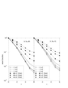
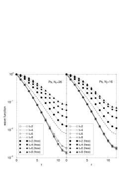
Figure 9: The results of “wave function” : dotted lines (full symbols) show free quark case, and dashed line (no symbol) show the initial shape of “wave function” i.e. shape of source function. The different symbols correspond to the different $t$ step. The result of pseudoscalar is left one, and that of vector is the other. The top figures are for Set-I and the bottom ones are for Set-II.

Fig. 9 shows the results at $T>0$ with the smeared source function which is slightly wider than the observed wave function at $T=0$. The wave functions composed of free quark propagators are also shown together.

As is shown in the Fig. 9, the behaviors of the observed wave functions are clearly different from that of the free quark case at each temperature and in each mesonic channel. In the free quark case the wave functions are broadening as $t$ as expected. On the other hand, the observed wave functions are stable with the slightly narrower shape than source function. These behaviors are independent of the source function.

For a visible expression, we define the averaged orbital radius, $r_{0}$, as

$$r_{0}^{3}(t)=\sum_{z}3z^{2}\phi_{M}(z,t),$$ (28)

where we suppose a spherical symmetric wave function and the sum is over $z$ axis. These $r_{0}(t)$ of Set-I and Set-II are shown in Fig. 10.

Figure 10: $t$ dependence of $r_{0}$. Left figure is for Set-I and right one is for Set-II.

Figure 10 shows the $t$ dependence of $r_{0}$ in the physical unit, where the error estimation takes into account the error of $a_{\sigma}$ and $a_{\tau}$. These results for Set-I and II are roughly consistent with each other. The behavior of observed $r_{0}$ are obviously different from free quark case, and shows the stable behavior with respect to $t$. This asymptotic value for the vector channel is larger than that of the pseudoscalar.

Below $T_{c}$, $r_{0}$ for each channel are almost same as the case of $T=0$. At $T\simeq 1.5T_{c}$ the observed $r_{0}$ are slightly larger than that of $T<T_{c}$. However the wave function, even in the deconfinement phase, seem to have the stable $r_{0}$ independently of the source function. Therefore we conclude the same strong spatial correlation as below $T_{c}$ survives in the deconfinement phase at each mesonic channel.

The results of this subsection seem to suggest the presence of the hadronic state in the deconfinement phase, at least up to $1.5T_{c}$. This is the opposite situation to the picture mentioned in the previous subsection.

6 Conclusion

In this paper we explored the charmonium correlators in the Euclidean temporal direction at $T>0$ using the quenched lattice QCD simulation. The high resolution in the temporal direction is achieved by employing the anisotropic lattice. We examined the thermal effect on the correlators based on the following two quantities: the correlators between the optimized operators tuned at $T=0$, and the $t$-dependence of $q\bar{q}$ wave function.

In the calculation of the wave function in the Coulomb gauge, we found the strong spatial correlation even above $T_{c}$, up to at least $1.5T_{c}$. These results indicate the quark and the anti-quark tend to be close each other even in the deconfinement phase. The similar result is reported in the light quark mass region in the Ref. [8]. In the case of charm quark mass these results suggest that the $J/\psi$ may not easily be resolved until $\sim 1.5T_{c}$. On the other hand, we also observed significant change of the nature of the correlators between the operators optimized at $T=0$. This was signaled by the drastic change of the behavior of effective mass. This situation is interesting, and at the same time puzzling. It is possible to consider several pictures which are able to explain our results. For example, the mesonic spectral function still have some peaks above $T_{c}$, and its width are broadened with thermal effects. Such a situation naturally explains the observed results in this work. The existence of hadronic modes just above $T_{c}$ were also suggested by the previous works[5]. From the analysis of temporal meson correlators at $T>0$, the QCD vacuum still has non-perturbative nature above the phase transition, and far from the perturbative plasma state of quark and gluon. In spite of several systematic uncertainties our results in the present work have important and interesting implications on the fate of hadronic states above the critical temperature.

Our approach is directly applicable to the dynamical configuration. If the full QCD simulation on the anisotropic lattice is appropriately implemented. Then it is interesting to investigate what effect our results receive from the dynamical quarks. To achieve the high resolution in the temporal direction, we adopted the anisotropic lattice and employed the O(a) improved Wilson quark action on it. These implementation also useful to study the heavy particle such as the glueballs[27] and scalar mesons. For the correlators of these states we are inevitably forced to extract the signals at the short time separation. The large temporal lattice cutoff enables us to simulate the heavy particles on lattices of moderate size with keeping the finite lattice cutoff effect small. The detailed information in the temporal direction is also significantly useful for the direct extraction of the spectral function from the lattice data. This approach may give us the further information on the spectral structure of mesons at $T>0$.

7 Acknowledgments

We thank the members of QCD-TARO Collaboration for interesting discussion. H.M. thanks T.Onogi, N.Nakajima and J.Harada for useful discussion. The simulation has been done on Intel Paragon XP/S and NEC HSP at the Institute for Nonlinear Science and Applied Mathematics, Hiroshima University, NEC SX-4 at Research Center for Nuclear Physics, Osaka University and Hitachi SR8000 at KEK. This work is supported by the Grant-in-Aide for Scientific Research by Monbusho, Japan ( No. 10640272, No. 11440080 ). H.M. is supported by the center-of-excellence (COE) program at RCNP, Osaka University.

References

- [1] NA50 Collaboration, Phys. Lett. B477 (2000) 28.
- [2] T. Matsui and H. Satz, Phys. Lett. B178 (1986) 416.
- [3] D.E. Groom et al.(Particle Data Group), Eur. Phys. Jour. C15 (2000) 1.
- [4] For recent review, see e.g. H. Meyer-Ortmanns, Rev. Mod. Phys. 68 (1996) 473.
- [5] C. DeTar, Phys. Rev. D32 (1985) 276; D37 (1988) 2328.
- [6] T. Hatsuda and T. Kunihiro, Phys. Rep. 247 (1994) 221.
- [7] C. DeTar and J.B. Kogut, Phys. Rev. D36 (1987) 2828.
- [8] QCD-TARO Collaboration (Ph. de Forcrand et al.), Nucl. Phys. (Proc. Suppl.) B73 (1999) 420; (Proc. Suppl.) B83 (2000) 411; hep-lat/0008005.
- [9] T. Hashimoto et al, Phys. Rev. Lett. 57 (1986) 2123.
- [10] A. El-Khadra, A. S. Kronfeld and P. B. Mackenzie, Phys. Rev. D55 (1997) 3933.
- [11] B. Sheikholeslami and R. Wohlert, Nucl. Phys. B259 (1985) 572.
- [12] T. R. Klassen, Nucl. Phys. (Proc. Suppl.) B73 (1999) 918.
- [13] P. Chen, hep-lat/0006019.
- [14] A. Ali Khan, et al (CP-PACS Collaboration), hep-lat/0011005
- [15] G. P. Lepage and P. B. Mackenzie, Phys. Rev. D48 (1993) 2250.
- [16] B.A. Thacker and G. P. Lepage, Phys. Rev. D43 (1991) 196.
- [17] F. Karsch, Nucl. Phys. B205 (1982) 285.
- [18] M. Lüscher and P. Weisz, Commun. Math. Phys. 97 (1985) 59; Erratum Commun. Math. Phys. 98 (1985) 433.
- [19] M. Fujisaki et al. (QCD-TARO Collaboration), Nucl. Phys. (Proc. Suppl.) B53 (1997) 426.
- [20] J. Engels, F. Karsch and T. Scheideler, Nucl. Phys. (Proc. Suppl.) B63 (1998) 427.
- [21] T. R. Klassen, Nucl. Phys. B533 (1998) 557.
- [22] E. Eichten et al, Phys. Rev. D21 (1980) 203.
- [23] C. Bernard et al, Phys. Rev. Lett. 68 (1992) 2125.
- [24] P. Boyle (UKQCD Collaboration), hep-lat/9903017.
- [25] N. H. Shakespeare and H. D. Trottier, Phys. Rev. D58 (1998) 034502.
- [26] A. El-Khadra, Nucl. Phys. (Proc. Suppl.) B30 (1993) 449.
- [27] C. J. Morningstar, M. Peardon, Phys. Rev. D56 (1997) 4043.