Non-perturbative Renormalization in Lattice Field Theory

Abstract

I review the strategies which have been developped in recent years to solve the non-perturbative renormalization problem in lattice field theories. Although the techniques are general, the focus will be on applications to lattice QCD. I discuss the momentum subtraction and finite volume schemes, and their application to scale dependent renormalizations. The problem of finite renormalizations is illustrated with the example of explicit chiral symmetry breaking, and I give a short status report concerning Symanzik’s improvement programme to O($a$).

1 INTRODUCTION

A Quantum Field Theory is renormalized by defining the infinite cutoff or continuum limit of the regularized theory. The procedure is familiar in perturbation theory, but is more generally applicable. In particular, the renormalization of asymptotically free theories at low scales requires a genuinely non-perturbative approach. Unfortunately there exist very few analytical tools, and numerical simulations of the lattice regularized theory are often the only method to obtain quantitative results.

One is thus led to discuss renormalization of the lattice field theory and to take the continuum limit based on numerical data. In general this is only possible by making assumptions about the continuum approach. Motivated by Symanzik’s analysis of the cutoff dependence in perturbation theory, one usually assumes that the contiuum limit is reached with power corrections in the lattice spacing $a$, possibly modified by logarithms. In this context “unexpected results” have been presented recently by Hasenfratz and Niedermayer [1, 2]. They find that the continuum approach of a renormalized coupling in the O(3) non-linear sigma model is compatible with being linear in $a$, rather than quadratic, as one would expect for a bosonic model. While the statistical precision of the data is quite impressive, it seems premature to draw conclusions. We also note that there are many results in (quenched) QCD which are well compatible with expectations, and some of them will be presented below. Finally, I will assume the “‘standard wisdom” concerning asymptotic freedom and the operator product expansion (OPE) to be correct. While this has never been established beyond perturbation theory, a numerical check of the OPE in the O(3) model has recently been presented in ref. [3]. For an unconventional point of view regarding asymptotic freedom I refer to ref. [4].

Despite the more general title I will focus on lattice QCD. For one, non-perturbative renormalization techniques in QCD have reached a mature stage, so that systematic errors can be discussed. Second, QCD is a typical example, and the techniques carry over essentially unchanged to other theories.

This article is organized as follows. In sect. 2, I sketch the non-perturbative renormalization procedure for QCD. Then the two classes of schemes are reviewed which have been proposed to solve the problem of scale-dependent renormalization, namely the momentum subtraction schemes (RI/MOM, sect. 3) and finite volume schemes derived from the Schrödinger functional (sect. 4). This is followed by a discussion of finite renormalizations (sect. 5), and O($a$) improvement (sect. 6). I conclude with a remark concerning power divergences.

2 NON-PERTURBATIVE RENORMALIZATION OF QCD

2.1 Determination of fundamental parameters

The free parameters of the QCD action are the bare coupling and the bare quark mass parameters. At low energies the theory is usually renormalized in a hadronic scheme, i.e. one chooses a corresponding number of hadronic observables which are kept fixed as the continuum limit is taken.

Once the theory has been renormalized in this way, no freedom is left and the renormalized parameters in any other scheme are predicted by the theory. Of particular interest is the relation to the renormalized coupling and quark masses in a perturbative scheme. This is equivalent to a determination of the $\Lambda$-parameter and the renormalization group invariant quark masses. For, given the running coupling $\bar{g}$ and quark masses $\overline{m}_{i}$ at scale $\mu$, one finds the exact relations

$$\Lambda = \mu\,(b_{0}\bar{g}^{2})^{-b_{1}/2b_{0}^{2}}\,\exp\left\{-\hbox{$1\over 2b_{0}\bar{g}^{2}$}\right\}$$

$$\times\exp\left\{-\int_{0}^{\bar{g}}{\rm d}x\left[\hbox{$1\over\beta(x)$}+\hbox{$1\over b_{0}x^{3}$}-\hbox{$b_{1}\over b_{0}^{2}x$}\right]\right\},$$

$$M_{i} = \overline{m}_{i}\,(2b_{0}\bar{g}^{2})^{-d_{0}/2b_{0}}$$ (2)

$$\times\exp\left\{-\int_{0}^{\bar{g}}{\rm d}x\left[\hbox{$\tau(x)\over\beta(x)$}-\hbox{$d_{0}\over b_{0}x$}\right]\right\},$$

where $i$ labels the quark flavours. Here, $\beta$ and $\tau$ are renormalization group functions with asymptotic expansions,

$$\beta(g) \sim -b_{0}g^{3}-b_{1}g^{5}+\ldots,$$ (3)

$$\tau(g) \sim -d_{0}g^{2}-d_{1}g^{4}+\ldots.$$ (4)

Note that the renormalization group invariant quark masses are scheme independent, whereas the Lambda parameter changes according to

$$\Lambda^{\prime}=\Lambda\exp\{c^{(1)}/b_{0}\}.$$ (5)

Here, $c^{(1)}$ is the one-loop coefficient relating the renormalized coupling constants $g^{\prime}=g+c^{(1)}g^{3}+{\rm O}(g^{5})$. $\Lambda$ in the $\overline{\rm MS}$ scheme and $M_{i}$ are referred to as the fundamental parameters of QCD.

In order to relate the hadronic scheme to these parameters one may introduce an intermediate renormalization scheme involving quantities which can be evaluated both in perturbation theory and non-perturbatively. An obvious possibility is to take a renormalized coupling and renormalized quark masses which are defined beyond perturbation theory. In such a scheme also the renormalization group functions $\beta$ and $\tau$ are defined non-perturbatively, so that the formulae (2.1,2) can be applied at any scale $\mu$, once the matching to the hadronic scheme has been performed.

2.2 Renormalization of composite operators

In the Standard Model composite operators often arise when the OPE is used to separate widely different scales in a physical amplitude. While the operators are originally defined at high energies (e.g. at $\mu=M_{W}$) and in a perturbative scheme, one is usually interested in their matrix elements between hadronic states. This defines a matching problem between a perturbative renormalization scheme for the operator (e.g. the $\overline{\rm MS}$ scheme) and a hadronic scheme, where a particular hadronic matrix element of the operator assumes a prescribed value.

The problem may again be approached by defining an intermediate renormalization scheme which can be evaluated both non-perturbatively and in perturbation theory. At high energies one may then either convert to a perturbative scheme, or one may construct the renormalization group invariant operator, in close analogy to the fundamental parameters introduced above.

2.3 The problem of scales

The main problem for the lattice approach is due to the large scale differences. In order to measure hadron masses the hadrons have to fit into the (necessarily finite) space-time volume, i.e. $L^{-1}\ll m_{\pi}$. On the other hand, the matching to the intermediate scheme is done via the bare parameters at a matching scale $\mu_{0}$, and one requires $\mu_{0}\ll a_{\rm max}^{-1}$, where $a_{\rm max}$ denotes the largest lattice spacing considered in the continuum extrapolation of the matching condition. As the available lattice sizes $L/a$ are limited, $\mu_{0}$ can not be too large, and perturbation theory at this scale may not be reliable. This ought to be checked by tracing the non-perturbative scale evolution of the renormalized parameters in the intermediate scheme. If the on-set of perturbative evolution is observed around a scale $\mu$, one may then apply the formulae (2.1,2) using the perturbative expressions (3,4).

Combining the various requirements, one gets

$$L^{-1}\ll m_{\pi},\Lambda\ll\mu\ll a^{-1},$$ (6)

and one also wants to vary $a$ in order to take the continuum limit. A naive estimate then leads to ratios $L/a={\rm O}(10^{3})$ which are clearly too large to be realised on a single lattice.

2.4 Shortcut methods

Given a hadronic scheme at fixed $g_{0}$ one may be tempted to avoid introducing the intermediate renormalization scheme by considering the bare coupling and the bare quark masses themselves as running parameters defined at the cutoff scale $a^{-1}$. One may then match directly to, say, the $\overline{\rm MS}$ scheme at scale $\mu=a^{-1}$, by using bare perturbation theory [5]. While this method is quick, it is also very difficult to estimate the error in a reliable way. In particular it is impossible to disentangle renormalization from cutoff effects, as any variation of $a$ is at the same time a variation of the renormalization scale.

3 THE RI/MOM SCHEME

The RI/MOM scheme [6] (RI for “regularization independent”) is a momentum subtraction scheme applied in a non-perturbative context [6, 7, 8, 9, 10, 11, 12, 13, 14]. It plays the rôle of an intermediate renormalization scheme in the sense of the previous section.

3.1 The renormalization procedure

In the RI/MOM scheme one considers correlation functions with external quark states in momentum space. A necessary first step therefore consists in fixing the gauge (usually Landau gauge). One then follows the same procedure as in perturbation theory: first the full quark propagator is computed for a set of momenta and then used to amputate the external legs of the correlation function of interest. The resulting vertex function is then considered as a function of a single momentum, and one imposes that its renormalized counterpart be equal to its tree-level expression at the subtraction point, viz.

$$\Gamma_{\rm R}(p)\bigl{|}_{p^{2}=\mu^{2}}=\Gamma(p)^{\rm tree}.$$ (7)

For example, in the case of a multiplicatively renormalizable quark bilinear operator $O$ eq. (7) determines the operator renormalization constant $Z_{O}(g_{0},a\mu)$ up to the quark wave function renormalization. The latter is then determined by considering the vertex function of a conserved current [6]. Note that the renormalization constant is usually assumed to be quark mass independent. This can be achieved by imposing the renormalization condition (7) in the chiral limit [15].

The RI/MOM scheme may also be used to obtain non-perturbatively defined renormalized parameters. The PCAC and PCVC relations imply that renormalized quark masses can be defined using the inverse renormalization constants of the axial or the scalar density. To define a renormalized gauge coupling one may allow for external gluon states and impose a RI/MOM condition on the 3-gluon vertex function [16, 17].

3.2 Matching to other schemes

Suppose one is interested in a hadronic matrix element of some operator $O$ defined in the $\overline{\rm MS}$ scheme. As a first step one relates the $\overline{\rm MS}$ scheme to the RI/MOM scheme by inserting the renormalized operator in the renormalization condition (7). This determines the finite renormalization constant $Z_{O}^{\overline{\rm MS}}$ relating the operators in the $\overline{\rm MS}$ and RI/MOM schemes, order by order in the renormalized coupling $g^{2}_{\overline{\rm MS}}(\mu)$.

Next, one computes the hadronic matrix element ${\cal M}(a)=\langle h^{\prime}|O|h\rangle$ for a sequence of lattice spacings and sets

$$Z_{O}^{\overline{\rm MS}}\left(g^{2}_{\overline{\rm MS}}(\mu)\right){\cal M}_{\overline{\rm MS}}(\mu)\mathrel{\mathop{=}^{\rm def}}\lim_{a\rightarrow 0}Z_{O}(a\mu){\cal M}(a).$$ (8)

where $\mu$ is fixed in terms of a hadronic scale and all mass parameters are supposed to be renormalized in a hadronic scheme. Here one has used the regularization independence of the RI/MOM condition to define the l.h.s. of this equation. Provided one has previously determined $g_{\overline{\rm MS}}(\mu)$ this completely specifies the matrix element in the $\overline{\rm MS}$ scheme to the calculated order in perturbation theory. Of course, it is assumed that continuum perturbation theory is applicable at the scale $\mu$. Whether this is the case can be checked by repeating the matching procedure at a different scale $\mu^{\prime}$. If the change is compatible with perturbative evolution from $\mu$ to $\mu^{\prime}$ one may use perturbation theory to run to larger scales and extract the renormalization group invariant matrix element.

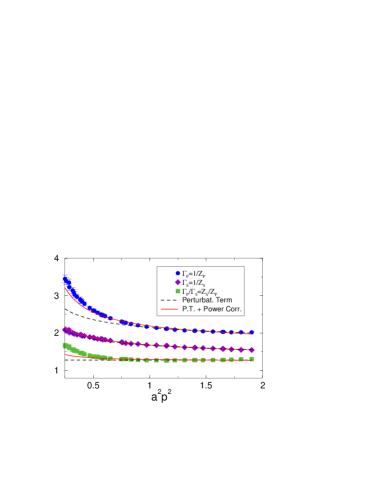
Figure 1: Non-perturbative vs. perturbative scale dependence of the renormalization constants of the scalar and axial density (ref. [12], improved Wilson fermions at $\beta=6.2$).

Figure 2: Renormalization of the quark mass with Kogut-Susskind fermions [11]. $Z_{m}$ should be $p$ independent if continuum perturbation theory was appropriate.

3.3 Examples

Typical examples of operator renormalizations are given in fig. 1, where the renormalization constants for the non-singlet axial and scalar densities are plotted against the renormalization scale, for O($a$) improved Wilson quarks in the quenched approximation at $\beta=6.2$ [12]. Also plotted are the curves obtained in continuum perturbation theory. As one observes good agreement with the perturbative curves, $p$-dependent cutoff effects are small and perturbation theory seems to apply at scales around $\mu\simeq 1/a(\beta=6.2)$.

In order to determine the light quark masses, the JLQCD collaboration renormalizes the scalar density using (quenched) Kogut-Susskind fermions at 3 $\beta$-values corresponding roughly to a variation of the cutoff by a factor of 2 [11]. The renormalization condition is extrapolated to the chiral limit, and the renormalized quark mass is related to the bare mass $m$ through

$$m_{\overline{\rm MS}}(\mu_{0})=\lim_{a\rightarrow 0}Z_{m}(\mu_{0},p,1/a)\,m$$ (9)

The total renormalization factor $Z_{m}$ consists of the non-perturbatively defined renormalization constant at scale $p$ and the perturbative 3-loop evolution factor relating the scales $p$ and $\mu_{0}$. If continuum perturbation theory was adequate between the scales $\mu_{0}=2\,{\rm GeV}$ and $p$, then $Z_{m}$ should be independent of $p$. This is not the case as fig. 2 demonstrates. However, if the continuum extrapolation of eq. (9) is performed for 2 different momenta $p=1.8\,{\rm GeV}$ and $p=2.6\,{\rm GeV}$, the results are nicely compatible, demonstrating that perturbation theory adequately describes the scale evolution in this range of scales. In particular, the window condition $\Lambda\ll\mu$ seems to be satisfied despite the absence of plateaux in fig. 2 at fixed $\beta$.

Further examples can be found in [7, 8, 9, 10, 11, 12, 13, 14]. In particular, the RBC collaboration has applied this scheme to the renormalization of operators in lattice QCD with Domain-Wall fermions [13, 14].

3.4 Merits and problems of the RI/MOM scheme

The RI/MOM scheme provides a versatile framework which can be easily adapted to new renormalization problems. Due to the regularization independence, perturbative calculations can be performed in a continuum scheme, with many results being already available. Furthermore, the use of external quark states is not only helpful in perturbation theory, but also leads to good signals in numerical simulations.

These nice properties come with a price: a non-perturbative gauge fixing procedure cannot avoid Gribov copies [18], and the RI/MOM renormalization conditions may introduce O($a$) effects into the otherwise on-shell O($a$) improved theory. Furthermore, the continuum perturbation theory is done in infinite space-time volume and in the chiral limit, whereas the numerical simulations are performed at finite quark masses and in a finite volume with periodic boundary condition. To satisfy the RI/MOM conditions chiral extrapolations are required and one ought to check for finite volume effects. Finally, the window condition $\Lambda\ll\mu\ll a^{-1}$ may not always be satisfied. In particular, problems may be expected with operators which couple to the pion. In fact, the JLQCD collaboration did not use the axial density in the quark mass renormalization, as the renormalization constant could not be extrapolated to the chiral limit [11]. This behaviour is attributed to a contribution of the Goldstone pole which should vanish at high enough scales [6]. For a more detailed discussion of this problem the reader is referred to refs. [19, 10].

3.5 Modifications of the RI/MOM scheme

At this conference, Y. Zhestkov (RBC collab.) has presented a first attempt to reach higher scales $\mu$ before matching to perturbation theory [13]. First results look promising, although it is not obvious how finite volume, renormalization and cut-off effects can be disentangled systematically. The situation could be simplified if the RI/MOM condition was imposed in a finite volume at constant $\mu L$. This would define a finite volume scheme, and finite-size scaling techniques could then be applied to reach higher scales. However, this means that all the perturbative calculations would have to be re-done in the finite volume set-up.

Finally, attempts are being made to implement off-shell O($a$) improvement of the quark vertex functions and propagators involved in the RI/MOM scheme. A short discussion is deferred to sect. 6.

4 FINITE VOLUME SCHEMES

4.1 Basic requirements

Finite volume schemes are obtained by using the finite extent of space-time to set the renormalization scale [20, 21], i.e. one identifies $\mu=L^{-1}$ in eq. (6). Using recursive finite size scaling methods one may bridge large scale difference, so that eq. (6) reduces to $a\ll L$ for any single lattice, and applicability of perturbation theory, $\Lambda\ll\mu$, is required only for the large scales (i.e. small $L$) covered by the recursion.

Finite volume schemes can be defined in many ways. However, one would like to maintain gauge invariance and respect on-shell improvement. Furthermore, the renormalization conditions should be easy to evaluate both by numerical simulation and in perturbation theory. A large family of renormalization schemes with all of these properties derives from the Schrödinger functional (SF) [22, 23] and is referred to as SF scheme.

4.2 The Schrödinger functional

The SF is the functional integral for QCD on a hyper-cylinder, i.e. all fields are $L$-periodic in the spatial directions, and satisfy Dirichlet boundary conditions at Euclidean times $0$ and $T$. For the quark fields one sets

$${P_{+}\psi|}_{x_{0}=0}= \!\!\rho,\qquad{P_{-}\psi|}_{x_{0}=T}= \!\!\rho^{\prime},$$

$${\bar{\psi}P_{-}|}_{x_{0}=0}= \!\!\bar{\rho},\qquad{\bar{\psi}P_{+}|}_{x_{0}=T}= \!\!\bar{\rho}^{\prime}\,,$$ (10)

with $P_{\pm}=\hbox{$1\over 2$}(1\pm\gamma_{0})$, and the spatial components of the gauge potential take prescribed values $C_{k}$ and $C^{\prime}_{k}$. Renormalizability of QCD in this situation has been discussed in [22, 24], with the result that the SF is finite after the usual renormalization of the parameters and multiplicative renormalization of all fermionic boundary fields by the same renormalization constant.

The SF is a gauge invariant functional of the boundary fields, ${\cal Z}={\cal Z}[\rho^{\prime},\bar{\rho}^{\prime},C^{\prime};\rho,\bar{\rho},C]$, and correlation functions may be defined as usual

$$\langle O\rangle=\left\{{\cal Z}^{-1}\int_{\rm fields}O\,{\rm e}^{-S}\right\}_{\rho=\rho^{\prime}=\bar{\rho}=\bar{\rho}^{\prime}=0},$$ (11)

where O may contain composite operators and boundary fields $\zeta,\bar{\zeta}$, which are obtained by differentiating with respect to the fermionic boundary values, e.g. $\zeta({\bf x})\rightarrow\delta/\delta\bar{\rho}({\bf x}).$ An important point to notice is that the gauge field boundary condition imply that only global gauge transformations are allowed at the boundaries. Bilinear boundary sources like $\bar{\zeta}({\bf x})\Gamma\zeta({\bf y})$ are therefore gauge invariant even for ${\bf x}\neq{\bf y}$.

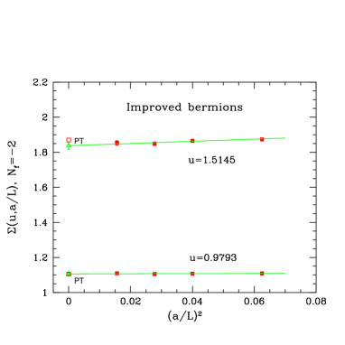
Figure 3: Continuum extrapolation of the step scaling function for the SF coupling with $N_{\rm f}=-2$, using O($a$) improved Wilson “bermions” [27].

4.3 Renormalized coupling

A non-perturbatively defined, gauge invariant running coupling can be obtained by choosing a family of boundary gauge fields depending on a parameter $\eta$ and setting [25]

$$\bar{g}^{2}(L)=\left.{\partial_{\eta}\Gamma_{0}}\over{\partial_{\eta}\Gamma}\right|_{\eta=0,m=0}.$$ (12)

Here, $\Gamma(\eta)=-\ln{\cal Z}[0,0,C^{\prime}(\eta);0,0,C(\eta)]$, is the effective action of the SF with the perturbative expansion,

$$\Gamma=g_{0}^{-2}\Gamma_{0}+\Gamma_{1}+g_{0}^{2}\Gamma_{2}+\ldots.$$ (13)

The numerator in eq. (12) thus ensures the standard normalization of a coupling constant. In eq. (12) $T=L$ is assumed, the boundary gauge fields are scaled with $L$ and the quark masses are set to zero. As a result the SF coupling is a quark mass independent coupling which runs with the scale $L$. Its perturbative relation to the $\overline{\rm MS}$ coupling is known to 2-loop order (cf. [26] and references therein).

For a completely different definition of a finite volume running coupling in the SU(2) pure gauge theory we refer to ref. [29].

4.4 Non-perturbative running

The coupling itself is an observable in numerical simulations, and the theory may now be renormalized in the chiral limit by imposing

$$\bar{g}^{2}(L)=u.$$ (14)

with some numerical value $u$. The coupling at scale $2L$ is then also determined and can be computed as a function of $u$ as follows. One chooses a lattice size $L/a$ and tunes $\beta$ such as to satisfy (14). Then one measures, at the same bare parameters, the SF coupling on a lattice with size $2L/a$. This yields a lattice approximant to the desired function, and by repeating these steps several times with increasing resolution $L/a$ one may take the limit,

$$\bar{g}^{2}(2L)=\sigma(u)=\lim_{a\rightarrow 0}\Sigma(u,a/L)\bigl{|}_{\bar{g}^{2}(L)=u,m=0}.$$ (15)

An example for such an extrapolation in QCD with $N_{\rm f}=-2$ (improved Wilson “bermions” [27]) is shown in fig. 3. Repeating the procedure with different values for $u$ the step-scaling function $\sigma(u)$ can be constructed in some interval $[u_{\rm min},u_{\rm max}]$. Setting $u_{0}=u_{\rm min}$, one computes recursively

$$u_{k}=\sigma(u_{k-1}),\quad k=1,2,\ldots,n.$$ (16)

In this way the scale evolution of the coupling is traced non-perturbatively and can be compared to perturbation theory (cf. figure 4). The ALPHA collaboration has determined the running in quenched QCD [25, 31] and is currently studying the theories with $N_{\rm f}=2$ and $N_{\rm f}=-2$ quark flavours. The corresponding computer programs for the APE1000 machine are being optimized, and the leftmost 3 points in fig. 4 have in fact been produced by the APE1000 as a warm-up exercise.

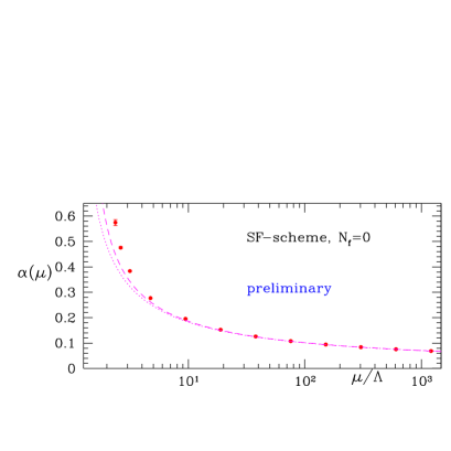
Figure 4: Non-perturbative running of the SF coupling ($N_{\rm f}=0$). For comparison also the perturbative 2-loop and 3-loop curves are shown.

4.5 Operator renormalization

To renormalize a composite operator in the SF scheme one starts by choosing a non-vanishing correlation with a boundary source field. In the case of the axial density $P^{a}=\overline{\psi}\hbox{$\tau^{a}\over 2$}\gamma_{5}\psi$ we define

$$O^{a}=a^{6}\sum_{{\bf y},{\bf z}}\bar{\zeta}({\bf y})\gamma_{5}\hbox{$\tau^{a}\over 2$}\zeta({\bf z}),$$ (17)

and similarly ${O^{\prime}}^{a}$ with the primed fields. Given the correlation functions

$$f_{\rm P}(x_{0})=-\hbox{$1\over 3$}\langle P^{a}(x)O^{a}\rangle,\quad f_{1}=-\hbox{$1\over 3L^{6}$}\langle O^{a}{O^{\prime}}^{a}\rangle,$$ (18)

one may then scale all dimensionfull parameters with $L$, and define the renormalization constant through the ratio [30]

$$Z_{\rm P}(g_{0},a/L)=c{\sqrt{f_{1}}\over{f_{\rm P}(L/2)}},$$ (19)

at vanishing quark masses. Here the ratio has been chosen such that the boundary field renormalization drops out, and the constant $c$ ensures $Z_{\rm P}=1$ to lowest order perturbation theory. One may then define the step scaling function for the renormalization constant,

$$\sigma_{\rm P}(u)=\lim_{a\rightarrow 0}\left.{{Z_{\rm P}(g_{0},2L/a)}\over{Z_{\rm P}(g_{0},L/a)}}\right|_{\bar{g}^{2}(L)=u,m=0}.$$ (20)

The equations,

$$Z_{\rm P}(2L)=\sigma_{\rm P}(u)Z_{\rm P}(L),\quad u=\bar{g}^{2}(L)$$ (21)

are then again solved recursively, using the previous result for the step-scaling function of the SF coupling [31].

4.6 Universality

The step-scaling functions are obtained in the continuum limit and do not depend on the regularization. This is illustrated in fig. 5, which shows the continuum extrapolation of two step scaling functions, defined in complete analogy with $\sigma_{\rm P}$. The simulations have been performed both with improved and unimproved Wilson fermions. Due to incomplete improvement residual O($a$) effects are expected in both cases, and the continuum extrapolated results nicely agree. [32].

In [33] an attempt is being made to relate the bare chiral condensate obtained with Neuberger fermions in [34] to the renormalized axial density in the SF scheme. If successful, the step scaling function $\sigma_{\rm P}$ could be used to extract the renormalization group invariant chiral condensate.

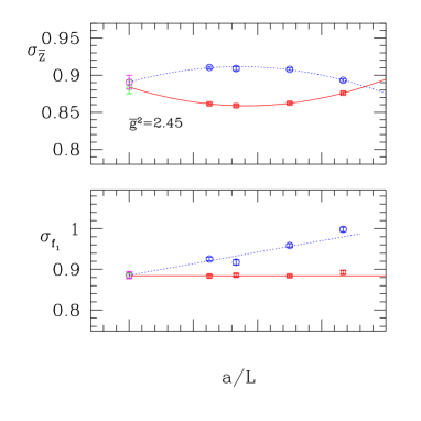
Figure 5: The continuum extrapolation of the two step-scaling functions of ref. [32] illustrate universality of the continuum limit. The lattice data were obtained with both O($a$) improved and unimproved Wilson fermions.

4.7 The static-light axial current

An interesting new development is the application of the SF techniques to QCD with an infinitely heavy “static” quark [35]. This is motivated by the fact that the $b$-quark is too heavy to be treated as a relativistic particle whilst maintaining a physically large volume. Applications to physics involving the b-quark therefore rely on large extrapolations in the quark mass, or on the use of effective theories, such as non-relativistic QCD or heavy quark effective theory. Controlling QCD in the limit of an infinitely heavy $b$-quark could lead to a major improvement for quantities like $F_{B}$, as the extrapolation in the quark mass is promoted to an interpolation.

In ref. [35] the SF for the static light theory has been defined in close analogy to the relativistic case. In particular it was found that the boundary quark fields are again multiplicatively renormalized. The application of Symanzik’s improvement programme reveals that the static action is already O($a$) improved and determines the structure of the improved static light axial current. In the effective theory the renormalization of the axial current is scale dependent and may be performed by imposing a similar condition as discussed above for the axial density. A potential problem is caused by the linear divergence stemming from self-energy corrections to the static quark. Fortunately, the contribution of this counterterm to the static quark propagator is exactly known. It is then possible to choose the ratios of correlation functions and parameters such that both the boundary field normalization and the self-energy counterterms cancel exactly.

The ALPHA collaboration has obtained the step-scaling function in the continuum limit, and the non-perturbative running of (a matrix element) of the current is shown in figure 6. The renormalization problem has thus been solved and work concerning the matrix element $F_{B}^{\rm stat}$ is in progress.

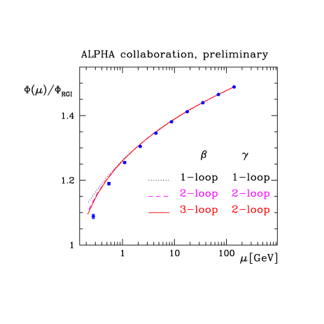
Figure 6: Non-perturbative running of the static-light axial current for $N_{\rm f}=0$. For comparison also the perturbative curves are shown [35].

5 FINITE RENORMALIZATIONS

In cases where a non-anomalous continuum symmetry is broken by the regularization, finite (i.e. scale independent) renormalizations are necessary to restore the symmetry up to cutoff effects. Well-known examples are the space-time symmetry, which is broken up to the discrete symmetry group of the space-time lattice, or global axial symmetries, which are completely broken in lattice QCD with Wilson quarks. In the case of chiral symmetry, the standard solution consists in imposing the validity of continuum chiral Ward identities in the theory at finite lattice spacing [36]. The same idea has been put foward in the case of supersymmetry by Curci and Veneziano [37], and first numerical and perturbative results along these lines have been presented at this conference [38, 39]. A similar treatment of the O(4) Euclidean space-time symmetry appears difficult in practice, as it requires the construction of the energy momentum tensor, which is a non-trivial problem in itself [40]. I will focus on the more familiar problem of explicit chiral symmetry breaking and its consequences.

5.1 Chiral symmetry and Wilson fermions

The explicit breaking of chiral symmetry by the Wilson term entails additive quark mass renormalization, a non-trivial renormalization of the non-singlet axial current,

$$(A_{\rm R})^{a}_{\mu}=Z_{\rm A}(g_{0})A_{\mu}^{a},$$ (22)

and mixing of operators with the wrong nominal chirality. For example, the $\Delta S=2$ operator

$$O^{\Delta S=2}=\sum_{\mu}\left(\bar{s}\gamma_{\mu}(1-\gamma_{5})d\right)^{2},$$ (23)

decomposes in parity even and parity odd parts,

$$O^{\Delta S=2}=O_{\rm VV+AA}-2\,O_{\rm VA}.$$ (24)

which are renormalized differently. While the parity odd operator is multiplicatively renormalized [41], the parity even operator mixes with four other operators of the same dimension,

$$O_{\rm VV+AA}^{\rm sub}=O_{\rm VV+AA}+\sum_{i=1}^{4}z_{i}(g_{0})O_{i}^{[d=6]},$$ (25)

and the subtracted operator is then multiplicatively renormalized.

In order to determine the scale independent renormalization constants $Z_{\rm A}$,$z_{i}$,$Z_{VV+AA}/Z_{VA}$, etc., Bochicchio et al. [36] have suggested to impose continuum axial Ward identities (AWI) as normalization conditions. A generic continuum AWI in the theory with $N_{\rm f}$ mass degenerate quarks has the form

$$\int_{R}{\rm d}^{4}x\left\langle\left(\partial_{\mu}A_{\mu}^{a}(x)-2mP^{a}(x)\right)O(y)O_{\rm ext}\right\rangle$$

$$+\left\langle\Bigl{(}\delta_{\rm A}^{a}O(y)\Bigr{)}O_{\rm ext}\right\rangle=0,$$ (26)

where $R$ is a finite space time region containing $y$, and $O_{\rm ext}$ is an arbitrary product of fields localized outside $R$. A simple example is the PCAC relation which is obtained for $O(y)=\delta(y-x)$. If imposed on the lattice it determines the additive quark mass renormalization constant. Considering axial variations of the axial current, the AWI’s determine the normalization constant $Z_{\rm A}$. More generally the axial Ward identities determine the relative renormalization of operators belonging to the same chiral multiplet, e.g. the scalar and axial densities, or $O_{\rm VA}$ and $O_{\rm VV+AA}$.

Applying AWI’s has become standard in the quenched approximation. At this conference, R. Horsley has presented a first attempt to determine $Z_{\rm A}$ for $N_{\rm f}=2$ flavours of O($a$) improved Wilson fermions [42].

The AWI’s can also be implemented more indirectly by applying the RI/MOM scheme to finite renormalization constants. With the appropriate choice for the renormalization conditions the AWI’s are automatically satisfied at large enough renormalization scales [43].

5.2 Systematic errors and O($a$) ambiguities

There is an infinity of axial Ward identities, and the results for a given scale independent renormalization constant will differ at O($a$) or O($a^{2}$), if the theory is O($a$) improved. One may be tempted to assign a systematic error to the renormalization constant corresponding to a “typical spread” of the results. This is somewhat subjective and unsatisfactory, in particular when the spread is large.

An alternative point of view has been advocated in refs. [44, 45]. One defines a given finite renormalization constant $Z$ by imposing the Ward identity at fixed renormalized parameters. As a result one obtains a smooth function of the bare coupling, $Z(g_{0})$, with relatively small errors.

When $Z(g_{0})$ is used in a continuum extrapolation the O($a$) ambiguity disappears in the limit. This can also be checked explicitly by choosing another renormalization condition which yields a different function $\tilde{Z}(g_{0})$. The difference $Z(g_{0})-\tilde{Z}(g_{0})$ must then vanish in the continuum limit, with an asymptotic rate proportional to $a$ or $a^{2}$. In ref. [45] the ALPHA collaboration has confirmed this expectation with the example of the finite renormalization constant $Z_{m}Z_{\rm P}/Z_{\rm A}$.

5.3 Avoiding finite renormalizations

Some of the scale-independent renormalizations with Wilson type quarks can be avoided by working in a different basis of fields. Such an approach has been presented at last year’s conference [46], and has been dubbed twisted mass QCD (tmQCD). One considers $N_{\rm f}=2$ quark flavours with the lattice action,

$$S_{\rm F}=a^{4}\sum_{x}\overline{\psi}(D_{W}+m_{0}+i\mu_{\rm q}\gamma_{5}\tau^{3})\psi.$$ (27)

Here, $D_{W}$ is the massless Wilson-Dirac operator, $m_{0}$ is the standard bare mass, and $\mu_{\rm q}$ is referred to as twisted mass parameter. This action has already appeared in the literature in different contexts [47, 48]. The new idea consists in renormalizing the theory at finite twisted mass, and in a re-interpretation of the renormalized theory as standard QCD with $N_{\rm f}=2$ mass degenerate quarks. If the renormalization scheme is chosen with care, the formulae relating renormalized tmQCD and standard QCD can be inferred from classical continuum considerations [49].

We thus consider the classical continuum lagrangian

$${\cal L}_{f}=\overline{\psi}\left(D\kern-7.0pt/+m+i\mu_{q}\gamma_{5}\tau^{3}\right)\psi+\bar{s}\left(D\kern-7.0pt/+m_{\rm s}\right)s.$$ (28)

where $\psi$ is a doublet of light quarks, and we have also included the strange quark. A chiral (non-singlet) rotation of the doublet fields,

$$\psi^{\prime} = \exp(i\alpha\gamma_{5}\tau^{3}/2)\psi,$$

$$\overline{\psi}^{\prime} = \overline{\psi}\exp(i\alpha\gamma_{5}\tau^{3}/2),$$ (29)

with $\tan\alpha=\mu_{\rm q}/m_{\rm q}$ transforms the Lagrangian to its standard form,

$${\cal L}^{\prime}_{f}(x)=\overline{\psi}^{\prime}(x)\left(D\kern-7.0pt/+m^{\prime}\right)\psi^{\prime}(x)+\bar{s}\left(D\kern-7.0pt/+m_{\rm s}\right)s,$$ (30)

with the light quark mass $m^{\prime}=(m^{2}+\mu_{\rm q}^{2})^{1/2}\,$. The rotation of the quark and anti-quark fields also induces a rotation of the composite fields. For quark bilinears containing only the light quarks one finds e.g.

$${A^{\prime}}_{\mu}^{1} = \cos(\alpha)A_{\mu}^{1}+\sin(\alpha)V_{\mu}^{2},$$ (31)

$$(\overline{\psi}\psi)^{\prime} = \cos(\alpha)\overline{\psi}\psi+2i\sin(\alpha)P^{3},$$ (32)

and the $\Delta S=2$ operator behaves as follows,

$$O_{\rm VV+AA}^{\prime}=\cos(\alpha)\,O_{\rm VV+AA}-2i\sin(\alpha)\,O_{\rm VA}.$$ (33)

The fields in the primed basis refer to the standard QCD basis, and the primed composite operators are hence interpreted as usual. Working in the twisted basis at $\alpha=\pi/2$ one may use the vector current to compute $F_{\pi}$, obtain the chiral condensate from $P^{3}$ and compute the $K-\bar{K}$ mixing amplitude using the multiplicatively renormalizable operator $O_{\rm VA}$ [41]. Work on tmQCD by the ALPHA collaboration is in progress, and the results of a scaling test have been presented at this conference [50].

A variant of the above proposal concerning $K-\bar{K}$ mixing can also be realized with standard Wilson fermions [51], by using the axial Ward identity (26). One considers an axial variation of $O=O_{\rm VA}$,

$$\delta_{\rm A}^{3}O_{\rm VA}=-\hbox{$1\over 2$}O_{\rm VV+AA},$$ (34)

and chooses $O_{\rm ext}$ as the product of interpolating fields for $K$ and $\bar{K}$. Imposing the AWI on the lattice is equivalent to defining the correlation function involving $O_{\rm VV+AA}$ through the remainder of the AWI, which contains the operator $O_{\rm VA}$. The trick here is that one directly obtains the desired matrix element by choosing $O_{\rm ext}$ appropriately. As in the tmQCD proposal this avoids solving the complicated mixing problem (25), and one is left with a scale dependent multiplicative renormalization for $O_{\rm VA}$. First feasibility tests have been performed and presented at this conference [52].

5.4 Ginsparg-Wilson and Domain-Wall quarks

Massless Ginsparg Wilson fermions are implicitly characterized by a Dirac operator which satisfies the Ginsparg-Wilson relation [53]

$$D\gamma_{5}+\gamma_{5}D=aD\gamma_{5}D.$$ (35)

The Ginsparg Wilson (GW) relation implies an exact chiral symmetry [54], and hence none of the finite renormalization constants discussed in this section is needed [55].

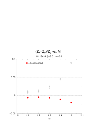
Figure 7: Difference between the axial and the vector current normalization constants as a measure of chiral symmetry violation [59].

An explicit solution of the Ginsparg-Wilson relation has been given by Neuberger [56]. Unfortunately, it is computationally very demanding to implement GW quarks exactly, and the question arises whether an approximation may be good enough in practice. A popular choice are Domain Wall fermions [57], which are formulated in five dimensions. The Dirac operator of the corresponding four-dimensional effective theory becomes an exact solution of the Ginsparg-Wilson relation as the number of lattice sites in the fifth dimension tends to infinity. As the approach is expected to be exponential, one may hope that a small number $N_{s}$ of points in the fifth dimension may already be sufficient.

To check the size of chiral symmetry violations one may pursue the same strategy as in the Wilson case, i.e. one measures to what extent chiral continuum Ward identities are violated. For example, one may measure the difference between vector current and axial current renormalization constants The CP-PACS collaboration has measured both renormalization constants using Ward identities at $m_{f}=0$, on a lattice of size $8^{3}\times 16\times 16$ (cf. fig. 7). The authors use the methods of ref. [44], and therefore impose SF boundary conditions in the physical time direction. Note, however, it that it is not obvious whether this is equivalent to imposing SF boundary conditions in the effective 4-dimensional theory.

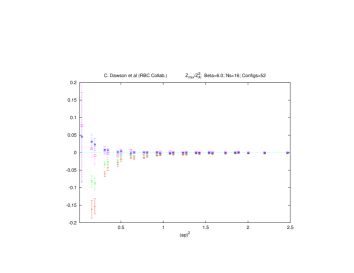
Figure 8: The wrong chirality mixing coefficients for the $\Delta S=2$ operator with domain wall fermions, as determined with the RI/MOM scheme [14].

The Riken-Brookhaven-Columbia (RBC) collaboration has studied the mixing properties of the operator $O_{\rm VV+AA}$ [14]. They follow ref. [60] and determine the wrong chirality mixing coefficients in a RI/MOM scheme. The result for $N_{s}=16$ is shown in fig. 8, and one observes that the coefficients are indeed small, i.e. a factor of 5-10 smaller than the corresponding result with (unimproved) Wilson quarks [61].

The overall impression is that chiral symmetry violations seem to be numerically small in many cases. However, it is also possible to determine the exponent of the exponential approach to a Ginsparg-Wilson solution directly by solving a generalized eigenvalue problem [62, 63]. It turns out that the exponent may be rather small at typical values of $\beta$, and with Wilson’s plaquette action for the gauge fields. This is potentially dangerous, and some modification of the original formulation of Domain Wall Fermions may be necessary (cf. [58] for further details).

6 O($a$) IMPROVEMENT

The purpose of Symanzik improvement [64, 65, 66] is to accelerate the continuum approach of renormalized quantities by introducing appropriate counterterms to both the action and the composite operators of interest. The counterterm structure follows from the symmetries of the regularized theory. Without loss of physical information improvement may be restricted to on-shell quantities, i.e. particle masses, energies and correlation functions of local operators which keep a physical distance from each other. In this case the equations of motion may be used to reduce the number of counterterms.

6.1 On-shell O($a$) improvement with Wilson quarks

The on-shell O($a$) improved action for $N_{\rm f}$ mass degenerate Wilson quarks is given by [67],

$$S_{\rm F}=a^{4}\sum_{x}\overline{\psi}(D_{W}+m_{0}+c_{\rm sw}a\hbox{$i\over 4$}\sigma_{\mu\nu}F_{\mu\nu})\psi,$$ (36)

where $D_{W}$ denotes the standard Wilson-Dirac operator. Other counterterms can be absorbed in the redefinition of the bare parameters. With the subtracted bare quark mass $m_{\rm q}=m_{0}-m_{\rm c}$, these are [68],

$$\tilde{g}_{0}^{2} = g_{0}^{2}(1+b_{\rm g}am_{\rm q}),$$ (37)

$$\widetilde{m}_{\rm q} = m_{\rm q}(1+b_{\rm m}am_{\rm q}),$$ (38)

and renormalized O($a$) improved parameters in a mass independent renormalization scheme take the form

$$g_{\rm R}^{2} = \tilde{g}_{0}^{2}Z_{\rm g}(\tilde{g}_{0}^{2},a\mu),$$ (39)

$$m_{\rm R} = \widetilde{m}_{\rm q}Z_{\rm m}(\tilde{g}_{0}^{2},a\mu).$$ (40)

Improved composite operators are treated similarly. We restrict attention to non-singlet quark bilinear operators, e.g. the axial current,

$$(A_{\rm R})_{\mu}^{a}=Z_{\rm A}(1+b_{\rm A}am_{\rm q})\left\{A_{\mu}^{a}+c_{\rm A}a\partial_{\mu}P^{a}\right\}.$$ (41)

The vector current and the tensor density have similar additive counterterms, and fields are multiplicatively rescaled with a quark mass dependent term and the appropriate $b$-coefficient. Note that all renormalization constants are functions of the improved bare coupling $\tilde{g}_{0}$, whereas the improvement coefficients depend on $g_{0}$.

6.2 O($a$) improvement and chiral symmetry

It is an important observation that all of the above counterterms conflict with chiral symmetry, and thus repair cutoff effects which originate from explicit chiral symmetry breaking. For this reason, lattice QCD with Ginsparg-Wilson quarks is on-shell O($a$) improved, provided the mass term is introduced in the correct way [69].

Concerning Wilson quarks it is a natural question whether axial Ward identities can be imposed as an improvement condition to determine the coefficients non-perturbatively. For those coefficients which already appear in the chiral limit (the $c$-coefficients), this is indeed the case: the integral over the region $R$ in eq. (26) can be converted into a surface integral over $\partial R$, and the axial Ward identity becomes an identity involving on-shell correlation functions only. Away from the chiral limit the answer is more subtle. The Ward identity now contains an off-shell correlation function, which is not expected to be improved.

An exception is the PCAC relation, which leads to an alternative definition of a renormalized O($a$) improved quark mass (40). Requiring equality of the two mass definitions then determines the combination

$$b_{\rm m}-b_{\rm A}+b_{\rm P}+g_{0}^{2}\,{\partial\ln Z\over\partial g_{0}^{2}}\,b_{\rm g},$$ (42)

where $Z=Z_{\rm m}Z_{\rm P}/Z_{\rm A}$ is a finite renormalization constant. Another special case is the coefficient $b_{\rm V}$ which may be determined from the vector Ward identities. Alternatively one may define an O($a$) improved current starting from the conserved current of the exact flavour symmetry, for which one finds $Z_{\rm V}=1$ and $b_{\rm V}=0$.

It is natural to ask whether the situation can be improved by allowing for mass non-degenerate quarks. Unfortunately the general counterterm structure becomes very complicated, i.e. there are many more possible $b$-coefficients [70]. Nevertheless, in the case $N_{\rm f}\geq 3$ these authors conclude that, assuming that $b_{\rm g}$ is known, all but three combinations of $b$-coefficients are indeed determined by Ward identities.

An independent proposal to determine the $b$-coefficients is based on the idea that chiral symmetry is restored at short distances [71]. This implies that the physical quark mass dependence is invariant under a sign change of the mass. As the $am_{\rm q}$ cutoff effects violate this invariance, one may in principle be able to isolate the coefficients. Unfortunately, in order to resolve sufficiently short distances one may need very small lattice spacings so that the method may not apply in the interesting range of $\beta$-values.

The situation becomes much simpler if one restricts attention to the quenched approximation. The coefficient $b_{\rm g}$ then vanishes and an improved bare quark mass parameter $\widetilde{m}_{\rm q}=m_{\rm q}(1+b_{\rm m}am_{\rm q})$ is defined for each flavour individually. Furthermore, the flavour off-diagonal quark bilinear fields are improved with the same $b$-coefficients as in the degenerate case, but with $m_{\rm q}$ replaced by the average of the valence quark masses in the operator [72, 73]. As shown in ref. [73] it is then indeed possible to determine all $b$-coefficients from axial Ward identities. In particular, off-shell correlation functions in the axial Ward identity are avoided by considering a partial chiral limit with two massless flavours and a further quark mass which is accompanied by the $b$-coefficient of interest.

6.3 Results

In perturbation theory the improvement coefficients are known to one-loop order [74, 75, 76, 77]. To this order the coefficients do not depend on $N_{\rm f}$ except for $b_{\rm g}$ [76]. Nonperturbative results have been obtained mostly in the quenched approximation with the exception of $c_{\rm sw}(N_{\rm f}=2)$ [78]. Numerical results exist for $c_{\rm sw}$  [79, 80], $c_{\rm A},b_{\rm V}$ [44] and $c_{\rm V}$ [81]. All these results were obtained by exploiting chiral Ward identities formulated in the Schrödinger functional, and in general the results are obtained as functions of $g_{0}$, for $\beta\geq 6.0$. In ref. [72] the combinations $b_{\rm A}-b_{\rm P}$ and $b_{\rm m}$ were determined for values $\beta\geq 6.2$, by considering the PCAC relation with non-degenerate quarks. Recently Bhattacharya et al. [82] have published the final version of their work with numerical results for all improvement coefficients needed for the improvement of quark bilinear operators. The numerical results are obtained at two $\beta$ values, $6.0$ and $6.2$, using hadronic correlation functions. An example is given in fig. 9.

Figure 9: The combination $b_{\rm A}-b_{\rm V}$ at $\beta=6.2$ is determined by the slope [82].

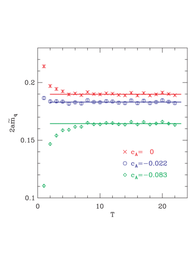
Figure 10: The improvement condition for the coefficient $c_{\rm A}$ at $\beta=6.0$ [82].

Figure 11: Simulation results and fit function for $b_{\rm A}-b_{\rm P}$, determined from an improvement condition imposed at constant physics [45].

Figure 12: The difference between two different determinations of $b_{\rm A}-b_{\rm P}$ at constant physics is plotted against $a/r_{0}$. One observes the expected decrease as the continuum limit is approached [45].

In general, the agreement with previous results is reasonably good, except for $c_{\rm V}$ and $c_{\rm A}$ at $\beta=6.0$. In particular, their preferred value for $c_{\rm A}$ is about $-0.04$ which is roughly half of the value obtained in [79]. Fig. 10 illustrates the sensitivity of the method: It shows the PCAC mass obtained from 2-point functions as a function of time separation. The excited states in the pion channel are sensitive to $c_{\rm A}$ which is tuned such as to extend the plateaux to smaller times. This procedure is repeated for various quark masses and an extrapolation to the chiral limit is performed. Similar results for $c_{\rm A}$ with essentially the same method have been obtained in ref. [83].

Improvement coefficients are intrinsically ambiguous by terms of O($a$). While a large O($a$) ambiguity in the case of $c_{\rm A}$ cannot be excluded, it may also be that the chosen improvement condition is afflicted by large higher order lattice artifacts, resulting in an artificial enhancement of the O($a$) ambiguity. In ref. [79] some checks were carried out to ensure that this does not happen and some alternative improvement conditions have corroborated the previous result for $c_{\rm A}$ at $\beta=6.0$ [84].

The ALPHA collaboration has extended the work of [72] and determined $b_{\rm m}$ and $b_{\rm A}-b_{\rm P}$ covering a range of values $\beta\geq 6.0$. Surprisingly, the $b_{\rm A}-b_{\rm P}$ coefficient shows a rather large O($a$) ambiguity. It was therefore decided to define the improvement condition at “constant physics”, keeping all quark masses and scales fixed in units of a physical scale (cf. sect. 5). The result for the final choice of the improvement condition is shown in figure 11. As expected the difference to an alternative definition decreases with a rate roughly $\propto a$ (cf. fig. 12).

6.4 Off-shell improvement of the gauge fixed theory

In order to render the RI/MOM scheme compatible with O($a$) improvement, one needs to extend improvement to the gauge fixed theory (Landau gauge), and to off-shell quantities, such as the vertex functions and quark propagators entering the RI/MOM renormalization conditions.

According to the authors of ref. [85] (cf. also [86]), this may be achieved by using the on-shell improved action supplemented with a gauge fixing term and the action of the ghost fields. Furthermore, one introduces additional O($a$) counterterms to the composite operators and the quark and anti-quark fields. In the case of gauge invariant quark bilinear operators the only additional counterterms are the ones which vanish by the equations of motion. Improvement of the quark field also requires the introduction of a non-gauge invariant counterterm $\propto a\partial{\kern-5.0pt}/\psi$ and an analogous term for the anti-quark field.

The latter counterterm is not needed in explicit one-loop calculations carried out in ref. [87]. These authors organize the calculation differently, by explicitly subtracting contact terms in the quark propagator and the vertex functions. However, this seems to be equivalent to the effect of those counterterms which vanish by the equations of motion. Finally we mention that some of the additional improvement coefficients for quark bilinear operators have been determined non-perturbatively in ref. [82].

7 CONCLUDING REMARKS

In the last few years a whole arsenal of tools has been created which will help to ultimately solve the non-perturbative renormalization problem of QCD and similar theories. In this talk I have tried to give an impression of the problems and the conceptual and technical progress in the field.

An important omission in this review concerns power divergences. The reason is that power divergences do not only present a technical but above all a serious conceptual challenge. To illustrate the potential problem, assume that QCD is regularized on the lattice with Ginsparg-Wilson quarks, and suppose we want to renormalize the isosinglet scalar density at non-zero quark mass. The structure of the renormalized operator is determined by the symmetries,

$$S^{0}_{\rm R}=Z_{\rm S}\left\{S^{0}+ma^{-2}c_{\rm S}(am,g_{0})\right\},$$ (43)

where $c_{\rm S}$ is a dimensionless coefficient which depends on the bare parameters and is independent of the renormalization scale $\mu$ [88]. To define the renormalized operator one should be able to impose a renormalization condition which does not refer to the regularization. In the chiral limit this is not a problem, as the additive renormalization vanishes exactly. At non-zero mass, however, one must first define a renormalized quark mass, which is only possible up to an intrinsic O($a^{2}$) ambiguity. The renormalization condition for the scalar density now refers to the renormalized quark mass, and one may be worried that the O($a^{2}$) ambiguity combines with the quadratic divergence to produce an O(1) ambiguity in the “renormalized operator”.

The example of the isosinglet scalar density may seem academic, but similar problems are expected in the renormalization of the effective weak hamiltonian. A theoretical solution to this problem might be Symanzik improvement to higher orders. However, this requires the introduction of four-quark operators in the action and does not seem very practical. New ideas may be necessary to either solve or circumvent these difficult renormalization problems, and an interesting new approach has already been proposed [89].

I would like to thank the conference organizers for the opportunity to give this talk. I have benefitted from discussions with many participants at the conference, and in particular with M. Lüscher, R. Petronzio, G.C. Rossi and R. Sommer. Furthermore I thank R. Sommer for critical comments on a draft of this writeup. Support by the European Commission under grant No. FMBICT972442 and by CERN is gratefully acknowledged.

References

- [1] P. Hasenfratz and F. Niedermayer, hep-lat/0006021
- [2] F. Niedermayer, these proceedings
- [3] S. Caracciolo et al., hep-lat/0007044
- [4] E. Seiler, these proceedings
-
[5]
see e.g.
C. Michael, Nucl. Phys. B (Proc. Suppl.) 42 (1995) 147 and references
therein;
C.T.H. Davies et al., Phys. Rev. D56 (1997) 2755 - [6] G. Martinelli et al., Nucl. Phys. B445 (1995) 81
- [7] V. Gimenez et al., Nucl. Phys. B531 (1998) 429
- [8] M. Göckeler et al., Nucl. Phys. B544 (1999) 699
- [9] A. Donini et al., Eur. Phys. J. C10 (1999) 121
- [10] L. Giusti and A. Vladikas, Phys. Lett. B488 (2000) 303
- [11] S. Aoki et al. (JLQCD Collaboration), Phys. Rev. Lett. 82 (1999) 4392
- [12] D. Becirevic et al., Nucl. Phys. (Proc. Suppl.) 83 (2000) 863
- [13] Y. Zhestkov (RBC coll.), these proceedings
- [14] C. Dawson (RBC coll.), these proceedings
- [15] S. Weinberg, Phys. Rev. D8 (1973) 3497
- [16] C. Parrinello, Phys. Rev. D50 (1994) 4217
- [17] B. Alles et al., Nucl. Phys. B502 (1997) 325
- [18] V. N. Gribov, Nucl. Phys. B139 (1978) 1
- [19] J. Cudell, A. Le Yaouanc and C. Pittori Phys. Lett. B454 (1999) 105
- [20] M. Lüscher, P. Weisz and U. Wolff, Nucl. Phys. B359 (1991) 221
- [21] K. Jansen et al., Phys. Lett. B372 (1996) 275
- [22] M. Lüscher et al., Nucl. Phys. B384 (1992) 168
- [23] S. Sint, Nucl. Phys. B421 (1994) 135
- [24] S. Sint, Nucl. Phys. B451 (1995) 416
- [25] M. Lüscher et al, Nucl. Phys. B413 (1994) 481
- [26] A. Bode, P. Weisz and U. Wolff [ALPHA collaboration], Nucl. Phys. B576 (2000) 517
- [27] J. Rolf and U. Wolff, Nucl. Phys. (Proc. Suppl.) 83 (2000) 899
- [28] ALPHA collaboration, work in progress
- [29] G. de Divitiis et al., Nucl. Phys. B422 (1994) 382
- [30] S. Sint and P. Weisz (ALPHA coll.), Nucl. Phys. B545 (1999) 529
- [31] S. Capitani et al., (ALPHA coll.), Nucl. Phys. B544 (1999) 669
- [32] M. Guagnelli, K. Jansen and R. Petronzio Phys. Lett. B457 (1999) 153
- [33] P. Hernandez et al., work in progress
- [34] P. Hernandez et al., Phys. Lett. B469 (1999) 198
- [35] M. Kurth and R. Sommer, hep-lat/0007002
- [36] M. Bochicchio et al., Nucl. Phys. B262 (1985) 331
- [37] G. Curci and G. Veneziano Nucl. Phys. B292 (1987) 555
- [38] A. Feo, these proceedings
- [39] F. Farchioni, these proceedings
- [40] S. Caracciolo et al., Annals Phys. 197 (1990) 119
- [41] C. Bernard et al., Nucl. Phys. (Proc. Suppl.) 4 (1988) 483.
- [42] R. Horsley (UKQCD & QCDSF collabs.), these proceedings
- [43] A. Donini et al., Eur. Phys. J. C10 (1999) 121
- [44] M. Lüscher et al., Nucl. Phys. B491 (1997) 344
- [45] M. Guagnelli et al. (ALPHA collab.), hep-lat/0009021
- [46] R. Frezzotti et al., Nucl. Phys. (Proc. Suppl.) 83 (2000) 941
- [47] S. Aoki, Phys. Rev. D30 (1984) 2653
- [48] W. Bardeen et al., Phys. Rev. D59 (1999) 014507
- [49] R. Frezzotti et al., to appear
- [50] Michele Della Morte, these proceedings
- [51] D. Becirevic et al., Phys. Lett. B487 (2000) 74
- [52] G. Martinelli, these proceedings
- [53] P.H. Ginsparg and K.G. Wilson, Phys. Rev. D25 (1982) 2649
- [54] M. Lüscher, Phys. Lett. B428 (1998) 342
- [55] P. Hasenfratz, Nucl. Phys. B525 (1998) 401
- [56] H. Neuberger, Phys. Lett. B417 (1998) 141
- [57] V. Furman and Y. Shamir, Nucl. Phys. B439 (1995) 54
- [58] P. Vranas, plenary talk (these proceedings)
- [59] CP-PACS collaboration, these proceedings
- [60] A. Donini et al., Phys. Lett. B360 (1995) 83
- [61] S. Aoki et al. (JLQCD collab.), Phys. Rev. D60 (1999) 034511
- [62] R.G. Edwards and U.M. Heller, hep-lat/0005002
- [63] P. Hernandez et al., hep-lat/0007015.
- [64] K. Symanzik, in: Mathematical problems in theoretical physics, eds. R. Schrader et al., Lecture Notes in Physics, Vol. 153 (Springer, New York, 1982)
- [65] K. Symanzik, Nucl. Phys. B226 (1983) 187 and 205
- [66] M. Lüscher and P. Weisz, Commun. Math. Phys. 97 (1985) 59, E: Commun. Math. Phys. 98 (1985) 433
- [67] B. Sheikholeslami and R. Wohlert, Nucl. Phys. B259 (1985) 572
- [68] M. Lüscher et al., Nucl. Phys. B478 (1996) 365
- [69] F. Niedermayer, Nucl. Phys. (Proc. Suppl.) 73 (1999) 105
- [70] T. Bhattacharya et al., Nucl. Phys. B (Proc. Suppl.) 83 (2000) 902
- [71] G. Martinelli et al., Phys. Lett. B411 (1997) 141
- [72] G. De Divitiis and R. Petronzio, Phys. Lett. B419 (1998) 311
- [73] T. Bhattacharya et al., Phys. Lett. B461 (1999) 79
- [74] R. Wohlert, DESY preprint 87-069 (1987), unpublished
- [75] M. Lüscher and P. Weisz, Nucl. Phys. B479 (1996) 429
- [76] S. Sint and R. Sommer, Nucl. Phys. B465 (1996) 71
- [77] S. Sint and P. Weisz, Nucl. Phys. B502 (1997) 251; Nucl. Phys. B (Proc. Suppl.) 63 (1998) 856
- [78] K. Jansen and R. Sommer, Nucl. Phys. B530 (1998) 185
- [79] M. Lüscher et al., Nucl. Phys. B491 (1997) 323
- [80] R.G. Edwards, U.M. Heller and T.R. Klassen, Nucl. Phys. (Proc. Suppl.) 63 (1998) 847
- [81] M. Guagnelli and R. Sommer Nucl. Phys. B (Proc. Suppl.) 63 (1998) 886
- [82] T. Bhattacharya et al., hep-lat/0009038
- [83] S. Collins, these proceedings
- [84] ALPHA collaboration, internal notes
- [85] G. Martinelli et al., unpublished
- [86] D. Becirevic et al., Phys. Rev. D61 (2000) 114507
- [87] S. Capitani et al., hep-lat/0007004.
- [88] M. Testa, JHEP 9804 (1998) 002
- [89] G. Martinelli, Nucl. Phys. B (Proc. Suppl.) 73 (1999) 58