Accelerating the Hybrid Monte Carlo algorithm
with ILU preconditioning.

Abstract

The pseudofermion action of the Hybrid Monte Carlo (HMC) algorithm for dynamical fermions is modified to directly incorporate Incomplete LU (ILU) factorisation. This reduces the stochastic noise and allows a larger molecular dynamics step-size to be taken, cutting the computational cost. Numerical tests using the two-flavour Schwinger model are presented, where a two-step ILU preconditioning of the even-odd fermion matrix allows the step-size to be increased by a factor of two over the standard even-odd formulation.

1 Introduction

Monte Carlo integration of the partition function of QCD with light quarks remains a computationally demanding task. At present, Hybrid Monte Carlo (HMC) [1] is amongst the most widely used algorithms for generating an ensemble of gauge field configurations with the dynamical QCD probability distribution. This exact algorithm combines molecular dynamics evolution in a fictitious simulation time, with a Metropolis test to ensure detailed balance. The effects of dynamical Wilson quark fields are introduced using gaussian-distributed “pseudofermion” fields and most of the computational effort goes into inverting the fermion matrix at each step of the molecular-dynamics trajectory. As a result, attention has focussed on improving the algorithms for this large, sparse matrix inversion.

ILU preconditioning schemes are commonly used to accelerate iterative inverters. For an interaction matrix, this translates into first ordering the sites on the lattice, then decomposing the matrix into upper and lower components. The upper segment couples a site only to those neighbours with a higher ordering index, and similarly the lower matrix couples to the lower-ordered sites. The preconditioning matrices are then constructed from these two terms. In one highly efficient inversion method for parallel machines, the SSOR scheme [2], a “locally-lexicographic” ILU preconditioning is used and the fermion matrix is subsequently inverted using BiCGStab. In Ref. [2], the commonly used even-odd (or “red-black”) scheme was recognised as an ILU decomposition, but not the optimal one. Even-odd (eo) preconditioning of the pseudofermion coupling matrix has also been used [3] to reduce the stochastic noise in molecular dynamics evolution, and leads to an increase in the acceptance rate of the Metropolis test. In this paper, it is first noted that, following the even-odd example, any ILU preconditioning can be applied directly to the matrix appearing in the pseudofermion action. Beyond this, a simple two-step scheme is presented, where the matrix is first even-odd preconditioned and the sites on one sub-lattice are subsequently ordered and ILU-factorised again. The global-lexicographic ordered version of this two-step scheme was proposed in Sec. 4 of Ref. [4]. In this work, other ordering schemes are tested. The two-step method leads to further improvements in the solver convergence rate and when used in the pseudofermion action, the HMC algorithm performance is also significantly enhanced.

The paper is organised as follows; Sec. 2 implements ILU preconditioning in the pseudofermion action and presents the two-level scheme, then in Sec. 3, these algorithms are tested in simulations of the Schwinger model. Here, using the two-step ILU preconditioned even-odd (eo-ILU) fermion matrix, a performance improvement of a factor of about two is found compared to the standard even-odd preconditioning. Sec. 4 briefly discusses application of the method in large-scale simulations on parallel computers and which use improved fermion actions.

2 Preconditioning the pseudofermions in HMC.

For simulations of a gauge theory with two degenerate flavours of dynamical fermions, the partition function is

$$Z=\int\!{\cal D}U\;\;\;\det M^{2}e^{-S_{g}},$$ (1)

with $S_{g}$ the lattice Yang-Mills discretisation and $\det M$ the determinant of the fermion matrix. In the HMC algorithm, this determinant is re-expressed as a gaussian integral over new bosonic degrees of freedom; the “pseudofermions”

$$\det M^{\dagger}M\equiv\int\!{\cal D}\phi^{*}{\cal D}\phi\;\;\;e^{-\phi^{*}\left[M^{\dagger}M\right]^{-1}\phi}.$$ (2)

Notice that to ensure the gaussian integral is well defined, the number of fermion flavours simulated must be even ($N_{f}=2$ is assumed throughout this work) and the $\gamma_{5}$-hermiticity property of the Wilson fermion matrix has been used; ie

$$M^{\dagger}=\gamma_{5}M\gamma_{5},\mbox{\hskip 21.52771pthence\hskip 21.52771pt}\det M=\det M^{\dagger}.$$ (3)

Then the partition function to be simulated is written as

$$Z=\int\!{\cal D}U{\cal D}\phi^{*}{\cal D}\phi\;\;\;e^{-S_{g}-\phi^{*}\left[M^{\dagger}M\right]^{-1}\phi}.$$ (4)

The Hybrid Monte Carlo algorithm generates a new element in the sequence of configurations in two stages. First, a fictitious continuous time variable, $\tau$ is introduced along with canonical momentum variables, $p_{\mu}(\mathbf{x})$ conjugate to each of the gauge degrees of freedom, $U_{\mu}(\mathbf{x})$. A hamiltonian describing dynamics in the new time coordinate is introduced,

$$H=\frac{1}{2}p^{2}+S_{g}+\phi^{*}\left[M^{\dagger}M\right]^{-1}\phi,$$ (5)

and the system is evolved in $\tau$ using a reversible, area-preserving integration scheme such as leap-frog. Since the integration scheme is inexact, the hamiltonian is not conserved and a subsequent stochastic step is added to compensate. After some time interval, the new configuration is proposed as an element of the ensemble and accepted or rejected according to the Metropolis test on the change in the hamiltonian;

$$P_{\rm acc}=\min(1,e^{-\delta H}).$$ (6)

The high computational cost of these dynamical fermion simulations arises as calculating the force term acting on the conjugate momenta at each leap-frog step requires two inversions of the fermion matrix, $M$.

An Incomplete LU (ILU) factorisation of $M$ was demonstrated as an efficient means of accelerating inversion [5, 2] and has been used successfully in large-scale production runs by eg. the SESAM collaboration [6]. The ILU factorisation preconditions the fermion matrix, $M$ by left and right multiplication with two readily invertible matrices;

$$\bar{M}=(I-L)^{-1}M(I-U)^{-1}$$ (7)

where $L$ and $U$ are the lower and upper parts of the Wilson hopping term. Defining $L$ and $U$ first requires the sites on the lattice, $\mathbf{x}$ are assigned an integer index, $s(\mathbf{x})$ then the site ordering is defined as

$$\mathbf{y}>\mathbf{x}\mbox{\hskip 12.91663ptif\hskip 12.91663pt}s(\mathbf{y})>s(\mathbf{x}),$$ (8)

with $\mathbf{y}<\mathbf{x}$ defined similarly. The lower part of the Wilson matrix is then

$$L_{\mathbf{x}\mathbf{y}}=\left(\begin{array}[]{cr}\kappa\sum_{\mu}U_{\mu}(\mathbf{x})(1-\gamma_{\mu})\delta_{\mathbf{y},\mathbf{x}+\mathbf{\hat{\mu}}}+U^{\dagger}_{\mu}(\mathbf{x}-\mathbf{\hat{\mu}})(1+\gamma_{\mu})\delta_{\mathbf{y},\mathbf{x}-\mathbf{\hat{\mu}}}&\mbox{when }\mathbf{y}<\mathbf{x}\\ 0&\mbox{otherwise}\end{array}\right.$$ (9)

and $U$ is defined similarly for sites where $\mathbf{y}>\mathbf{x}$. The full Wilson matrix is then equivalent to

$$M=I-L-U.$$ (10)

Matrix inversion is accelerated since the new matrix, $\bar{M}$ is better conditioned than $M$. The preconditioning matrices, $(I-L)$ and $(I-U)$ are easily inverted by either forward or backward substitution respectively. The $\gamma_{5}$-hermiticity (cf. Eqn. 3) of the preconditioned matrix is preserved as

$$\bar{M}^{\dagger}=\gamma_{5}\bar{M}\gamma_{5}\mbox{\hskip 21.52771ptsince\hskip 21.52771pt}(I-L)^{\dagger}=\gamma_{5}(I-U)\gamma_{5}.$$ (11)

Matrix-vector operations proceed efficiently via the “Eisenstat trick” [7, 2]; using Eqns. (7) and (10), $\bar{M}$ is re-written as

$$\bar{M}=(I-U)^{-1}+(I-L)^{-1}\left(I-(I-U)^{-1}\right),$$ (12)

and the matrix operation is reduced to a backward substitution followed by a forward one. This requires approximately the same number of floating point operations as the original Wilson matrix-vector product.

While the introduction of the pseudofermions to model the fermion determinant makes the molecular dynamics of the hamiltonian tractable, it also introduces extra randomness into this evolution. Simulations demonstrate that the Metropolis acceptance rate is higher with the better-conditioned even-odd matrix. For this study, first note that any ILU decomposition can be applied directly to the determinant of dynamical fermion simulations;

$$\det\bar{M}=\det(I-L)^{-1}\det(I-L-U)\det(I-U)^{-1}=\det M,$$ (13)

since $\det(I-L)=\det(I-U)=1$. From this identity, the fermion determinant can be simulated using pseudofermions coupled via the preconditioned matrix, $\bar{M}$

$$Z=\int\!{\cal D}U{\cal D}\phi^{*}{\cal D}\phi\;\;\;e^{-\phi^{*}\left[\bar{M}^{\dagger}\bar{M}\right]^{-1}\phi}.$$ (14)

The HMC algorithm can be applied to this new pseudofermionic partition function and the better conditioning of the matrix should lead to an improvement in the acceptance rate. The extent of this improvement will depend on the site ordering used, while physical expectation values computed on the ensemble will not. This will be tested in Sec. 3

2.1 Molecular dynamics for the preconditioned action.

The new hamiltonian generating the molecular dynamics is

$$\bar{H}=\frac{1}{2}p^{2}+S_{g}+\phi^{*}\left[\bar{M}^{\dagger}\bar{M}\right]^{-1}\phi,$$ (15)

In order to perform the molecular-dynamics updates, the force term acting on the momenta of the hamiltonian of Eqn. (15) must be determined. To demonstrate that the force term for the ILU preconditioned matrix, $\bar{M}$ is readily implemented, first note that the force arising from the gauge action is trivially left unchanged and consider the term arising from the pseudofermionic action alone,

$$\bar{S}_{\rm pf}=\phi^{*}\left[\bar{M}^{\dagger}\bar{M}\right]^{-1}\phi.$$ (16)

The derivative of this action with respect to $\tau$, keeping $\phi$ fixed is

$$\frac{d\bar{S}_{\rm pf}}{d\tau}=-\phi^{*}\left[\bar{M}^{\dagger}\bar{M}\right]^{-1}\left[\frac{d\bar{M}^{\dagger}}{d\tau}\bar{M}+\bar{M}^{\dagger}\frac{d\bar{M}}{d\tau}\right]\left[\bar{M}^{\dagger}\bar{M}\right]^{-1}\phi.$$ (17)

Introducing the auxiliary fields, $Y=\bar{M}^{\dagger-1}\phi$ and $X=\bar{M}^{-1}Y$, this becomes

$$\frac{d\bar{S}_{\rm pf}}{d\tau}=-Y^{*}\frac{d\bar{M}}{d\tau}X-X^{*}\frac{d\bar{M}^{\dagger}}{d\tau}Y.$$ (18)

At each leap-frog step, the fields $Y$ and $X$ must be recomputed; this is the section of the update requiring most of the computational effort. Note that the inversion proceeds more rapidly than in the original HMC algorithm as $\bar{M}$ is better conditioned. The derivative of $\bar{M}$ can be expanded after two new auxiliary fields are introduced; they are

$$Y_{L}=(I-L^{\dagger})^{-1}Y\mbox{\hskip 17.22217ptand\hskip 17.22217pt}X_{U}=(I-U)^{-1}X.$$ (19)

Note that constructing these fields requires only two backward substitutions ($L^{\dagger}$ is an upper-diagonal matrix), rather than an iterative method and so is an insignificant overhead compared to re-evaluating $X$ and $Y$. With these new fields, and using the definition of $\bar{M}$ in Eqn. (7), the derivative becomes

$$\frac{d\bar{S}_{\rm pf}}{d\tau}=-\left(Y_{L}^{*}\frac{dM}{d\tau}X_{U}+\phi^{*}\frac{dU}{d\tau}X_{U}+Y_{L}^{*}\frac{dL}{d\tau}Y+\mbox{ h.c.}\right).$$ (20)

Now derivatives of the original Wilson matrix, $M$ and its upper and lower sections appear in Eqn. (20) and so calculating the relevant force terms proceeds straightforwardly from here.

2.2 Even-odd (eo) and two-stage (eo-ILU) preconditioning

In Ref. [2], it was demonstrated that the commonly used even-odd preconditioning of the fermion matrix can be written as an ILU decomposition where the ordering function, $s(\mathbf{x})$ is simply 0 on even lattice sites and 1 on odd sites. There is no ordering ambiguity for the sites on the even or odd sub-lattices since $M$ does not contain hopping terms that directly couple sites on the same sub-lattice. For this example, the inversion of $(I-L)$ and $(I-U)$ can be written explicitly.

The preconditioned matrix is

$$\bar{M} = \left(\begin{array}[]{cc}I_{oo}&0\\ \kappa\Delta_{eo}&I_{ee}\end{array}\right)\left(\begin{array}[]{cc}I_{oo}&-\kappa\Delta_{oe}\\ -\kappa\Delta_{eo}&I_{ee}\end{array}\right)\left(\begin{array}[]{cc}I_{oo}&\kappa\Delta_{oe}\\ 0&I_{ee}\end{array}\right)$$ (27)

$$= \left(\begin{array}[]{cc}I_{oo}&0\\ 0&I_{ee}-\kappa^{2}\Delta_{eo}\Delta_{oe}\end{array}\right).$$ (30)

Pseudofermion degrees of freedom on the odd sites are completely decoupled from the gauge fields and can be discarded. The pseudofermions on even sites are then coupled via the sub-matrix, $M_{ee}=I_{ee}-\kappa^{2}\Delta_{eo}\Delta_{oe}.$

Since $M_{ee}$ is “ultra-local” (the only non-zero elements of the matrix couple sites within a small neighbourhood) and its elements can be written explicitly, it can be ILU preconditioned once again. The global lexicographic version of this second level of preconditioning was investigated in Section 4 of Ref. [4]. If a new ordering function, $s_{e}(\mathbf{x}_{e})$ is defined for sites on the even sub-lattice, then the (two-step) eo-ILU preconditioned matrix is

$$\bar{M}_{ee}=(I-L_{ee})^{-1}M_{ee}(I-U_{ee})^{-1},$$ (31)

with

$$L_{ee}=\kappa^{2}\sum_{\mathbf{y}_{e}<\mathbf{x}_{e}}\left.\Delta_{eo}\Delta_{oe}\right|_{\mathbf{x}_{e},\mathbf{y}_{e}}.$$ (32)

As before, the matrix determinant is left unchanged by this second level of preconditioning;

$$\det\bar{M}_{ee}=\det M_{ee}=\det M.$$ (33)

From here, a two-step preconditioned pseudofermion action can be implemented in the HMC algorithm, following a similar construction to Sec. 2.1. The new pseudofermion action is

$$\bar{S}_{\rm e}=\phi_{e}^{*}\left[\bar{M}_{ee}^{\dagger}\bar{M}_{ee}\right]^{-1}\phi_{e},$$ (34)

and, after introducing the auxiliary fields (on even sites only) $Y_{e}=\bar{M}_{ee}^{\dagger-1}\phi_{e}$ and $X_{e}=\bar{M}_{ee}^{-1}Y_{e}$ the derivative with respect to $\tau$ becomes

$$\frac{d\bar{S}_{\rm e}}{d\tau}=-Y_{e}^{*}\frac{d\bar{M}_{ee}}{d\tau}X_{e}-X_{e}^{*}\frac{d\bar{M}_{ee}^{\dagger}}{d\tau}Y_{e}.$$ (35)

Finally, after introducing the new fields $Y_{Le}=(I-L_{ee}^{\dagger})^{-1}Y_{e}$ and $X_{Ue}=(I-U_{ee})^{-1}X_{e}$, the derivative is

$$\frac{d\bar{S}_{\rm pf}}{d\tau}=-\left(Y_{Le}^{*}\frac{dM_{ee}}{d\tau}X_{Ue}+\phi_{e}^{*}\frac{dU_{ee}}{d\tau}X_{Ue}+Y_{Le}^{*}\frac{dL_{ee}}{d\tau}Y_{e}+\mbox{ h.c.}\right).$$ (36)

This expression contains derivatives of the original even-odd matrix and its lower and upper components. The first term is efficiently computed using the reconstruction trick; $Y_{L}$ and $X_{U}$ are defined on odd sites as $X_{Uo}=\kappa\Delta_{oe}X_{Ue}$ and $Y_{Uo}=\kappa\Delta^{\dagger}_{oe}Y_{Ue}$ then

$$Y_{Le}^{*}\frac{dM_{ee}}{d\tau}X_{Ue}\equiv Y_{L}^{*}\frac{dM}{d\tau}X_{U}$$ (37)

and so the force term is readily computed. Unfortunately no such reconstruction can be used for the terms involving $U_{ee}$ and $L_{ee}$. The reconstruction trick relies on the observation that the preconditioning matrices for the even-odd decomposition can be computed explicitly (as in Eqn. 30). While these algebraically cumbersome force terms must be evaluated explicitly, their evaluation is still a simple, local computational task.

3 Testing the method: the Schwinger model

To investigate the benefits of preconditioning, simulations of the two-flavour Schwinger model were performed. This model is a $U(1)$ gauge theory in $1+1$ dimensions and is a convenient testing ground for algorithms intended for full QCD simulations as it is asymptotically free, confining and has a spontaneously broken chiral symmetry. The link variables are phases; $U_{\mu}(\mathbf{x})=\exp\;i\theta_{\mu}(\mathbf{x})$ and for this study, the compact $U(1)$ gauge action is used

$$S_{g}=\beta\sum_{\Box}1-\cos\theta_{\Box},$$ (38)

with $\theta_{\Box}$ the sum of angles around the plaquette.

3.1 ILU orderings

Ref. [2] noted that the performance of ILU preconditioned inversion depends on the choice of ordering of the lattice sites. To study this, the spectral properties of the matrix were determined for a number of different schemes. The smallest and largest eigenvalues (and hence the condition number) of the hermitian matrix, $\bar{Q}$ ($\equiv\gamma_{5}\bar{M}$) were computed on an ensemble of 100 dynamical $\beta=4.0,\kappa=0.26,32\times 32$ lattices. The orderings tested were the standard even-odd checkerboard, a locally lexicographic (ll) scheme and a strip-lexicographic (sl) scheme. For the $(ll_{n})$ ordering, the lattice is first decomposed into an even-odd checkerboard of $n\times n$ blocks then the sites in each block are indexed starting at the corner with smallest coordinates and progressing first along the $x$-axis until the end of the block is reached before moving onto the next $y$ value. Note that $(ll_{1})$ is just the traditional even-odd indexing and $(ll_{N})$, where $N$ is the lattice extent, denotes a global lexicographic ordering. The $(sl)$ ordering first breaks the lattice into $1\times N$ strips and then the sites on each strip are indexed in order. Fig. 1 illustrates these ordering schemes on a $4\times 4$ lattice.

Figure 1: The index function, $s(x)$ for various lattice preconditionings. Grey shading denote areas that are lexicographically ordered. (a) is the standard even-odd preconditioning, denoted $ll_{1}$ (b) is the locally lexicographic scheme with block size 2, $ll_{2}$ and (c) is the strip-lexicographic scheme, $sl_{1}$.

Ordering	$|\lambda|_{\rm min}$	$|\lambda|_{\rm max}$	${\cal C}$	$n_{\rm iter}$
None	0.01768(48)	2.02173(11)	123.7(3.7)	501(11)
eo ($ll_{1}$)	0.03511(94)	1.56235(76)	48.1(1.4)	202(5)
$ll_{2}$	0.0419(11)	1.9873(14)	51.2(1.5)	104(3)
$ll_{4}$	0.0439(11)	2.8837(29)	70.7(2.2)	66.3(3)
$ll_{N}$	0.0444(11)	4.706(15)	114.0(3.5)	49.1(3)
$sl_{1}$	0.0443(12)	2.7254(23)	66.4(2.0)	104(1)

Table 1: Spectral properties of $\bar{M}$ (and $\bar{Q}$) at $\beta=4.0,\kappa=0.26$ on a $32\times 32$ lattice for various ILU schemes. The labelling of the ILU schemes is described in the text. Results for the schemes with optimal condition number and solver performance are in bold.

Table 1 presents the spectral properties of the hermitian fermion matrix, $\bar{Q}$ for a number of these schemes computed on 100 dynamical configurations. The eigenvalues of $\bar{Q}$ with the largest and smallest magnitudes are given, along with their ratio, ${\cal C}$ and $n_{\rm iter}$, the number of BiCGStab iterations required to invert the fermion matrix. All the eigenvalues of $\bar{Q}$ were computed using the Lanczos algorithm with reorthogonalisation. Their reliability was checked by testing $\det\bar{Q}=\det Q$ configuration-by-configuration. This relation was seen to hold to machine precision. Note that to ensure consistently accurate solutions in column 5, $|Mx-y|/|y|<10^{-12}$ was used as the stopping criterion for the BiCGStab solver (ie. the reconstructed residual of $M$ rather than $\bar{M}$).

These results confirm that the condition number of the preconditioned matrix and the solver performance is strongly dependent on the site ordering scheme. An unusual pattern emerges however; the preconditioning that leads to optimal solver performance (measured by the number of iterations required for convergence) is the global lexicographic scheme, $ll_{N}$ but the scheme with the lowest condition number is the standard even-odd decomposition. These two optimal orderings are highlighted in Table 1. The $ll_{N}$ inverter out-performs the even-odd method by a factor of four in iterations.

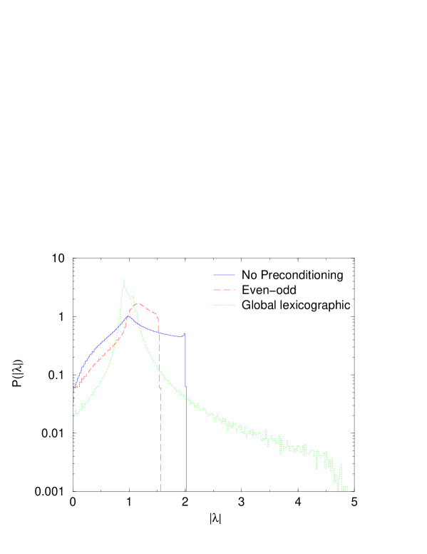
Figure 2: The eigenvalue probability distribution of $Q$ and $\bar{Q}$.

The mis-match between the optimal ordering for better conditioning and for inversion may be explained by closer examination of the eigenvalue spectrum. Fig. 2 shows the density of (the absolute value of) the eigenvalues of $Q$ without preconditioning and using even-odd and global lexicographic ILU schemes. For the $(ll_{N})$ scheme, most of the eigenvalues are distributed close to unity while a small number lie in a long tail stretching out to $|\lambda|=5$. This tail, while responsible for the high condition number is sparsely populated and so easily handled by the BiCGStab algorithm. The even-odd matrix has a hard upper bound on its eigenvalues and so is better conditioned, but these eigenvalues are broadly distributed inside that band. Note also that the performance results in Table. 1 are for inversion of $M$, not $Q$. The spectrum of $M$ has eigenvalues that are generally complex and has not been computed here; solver performance may depend on the eigenvalue distribution in the complex plane. A heuristic argument for the better performance of the global-lexicographic ordering can be made by noting that each iteration of the solver couples every site on the lattice with every other site.

3.2 ILU HMC algorithm performance

The ordering schemes of Sec. 3.1 were used to precondition the matrix coupling pseudofermions in a set of dynamical fermion simulations on lattices of size $32\times 32$. The gauge coupling was fixed to $\beta=4.0$ throughout. For the computations of the $X$ and $Y$ fields, the BiCGStab algorithm was again used (the stopping criterion was based on the residual of the preconditioned solution vector, to reduce computational overheads). In the molecular dynamics leap-frog step, the Sexton-Weingarten integrator scheme [8] was implemented. Here, the force on the conjugate momenta is separated into two parts; one arising from the pseudofermion action and the other from the Yang-Mills term of Eqn. (38). By interleaving the different momenta and gauge field updates, the step-size used for integrating the Yang-Mills force term, $d\tau_{g}$ is then made smaller than the step-size for the pseudofermionic force, $d\tau_{f}$. This isolates any changes in the update hamiltonian arising from the preconditioned fermion determinant. For all simulations, $d\tau_{g}=\frac{1}{4}d\tau_{f}$ was used. This value was chosen in some short tests and subsequently found to be sufficient to remove the finite-step-size effects of the gauge action in all runs. The molecular-dynamics trajectory length was selected randomly in the interval $\frac{1}{2}<\tau<1\frac{1}{2}$ to ensure ergodicity.

Table 2 shows the expectation values of the $1\times 1$ and $4\times 4$ Wilson loops from simulations using the preconditioning orderings of Sec. 3.1. All simulations were performed on a $32\times 32$ lattice, at $\beta=4.0,\kappa=0.2600$. Wilson loop averages agree within statistical uncertainties, as expected. Also in Table 2 are the acceptance probabilities of the final Metropolis test at the end of each molecular dynamics trajectory and (for reference) the condition numbers, ${\cal C}$ from Table. 1 are included. While all the ILU preconditioned simulations outperform the standard HMC algorithm, there is little variation among the different orderings. The optimal schemes use even-odd and strip-lexicographic ordering. The global-lexicographic scheme, while the best ordering for inversion, is the worst for HMC performance. It is possible that the higher condition number of $\bar{Q}$ in this scheme, due to the long tail of eigenvalues seen in the spectrum of Fig. 2, leads to instabilities in the molecular-dynamics evolution at a smaller step-size. Notice there is a correlation between the highest acceptance rates and the lowest condition numbers.

Ordering	$N_{\rm sweep}$	$\langle W(1,1)\rangle$	$\langle W(4,4)\rangle$	${\cal P}_{\rm acc}$	${\cal C}$
None	5000	0.87348(41)	0.1800(31)	0.120(11)	123.7(3.7)
eo $(ll_{1})$	10000	0.87407(14)	0.18542(82)	0.7310(74)	48.1(1.4)
$ll_{2}$	1000	0.87420(43)	0.1815(25)	0.721(17)	51.2(1.5)
$ll_{4}$	1000	0.87416(34)	0.1834(27)	0.691(16)	70.7(2.2)
$ll_{N}$	1000	0.87413(48)	0.1842(30)	0.647(21)	114.0(3.5)
$sl_{1}$	1000	0.87360(37)	0.1826(27)	0.745(14)	66.4(2.0)

Table 2: Wilson loop expectation values and acceptance probabilities from simulations using different preconditioning site ordering schemes. All simulations were performed on $32\times 32$ lattices at $\beta=4.0,\kappa=0.26$ with an MD step-size of $d\tau=\frac{1}{24}$.

3.3 eo-ILU preconditioning

Sec. 2.2 introduced a two-step preconditioning scheme (eo-ILU), where initially an even-odd decomposition of the fermion matrix is applied, followed by an ILU preconditioning. In the second step, an ordering scheme for the sites on the even (or odd) sites only is defined. In this section, the performance of the BiCGStab solver and HMC algorithm on eo-ILU matrices is presented. Three ordering schemes are tested; the first is the standard global-lexicographic scheme and the second two are the two local preconditionings, labelled A and B, which are the extension of even-odd preconditioning on the sub-lattice. In order to avoid ambiguity, four “flavours” of sub-lattices must be defined, since the even-odd matrix couples the eight sites with off-set vectors $\{\pm 1,\pm 1\},\{\pm 2,0\}$ and $\{0,\pm 2\}$. These three preconditionings are illustrated for a $4\times 4$ lattice in Fig. 3.

Figure 3: Two-step eo-ILU preconditioning schemes. (a) and (b) are the two distinct local decompositions, (in two dimensions). In (c) the entire even sub-lattice is lexicographically ordered.

Ordering	$|\lambda|_{\rm min}$	$|\lambda|_{\rm max}$	${\cal C}$	$n_{\rm iter}$
None	0.02306(77)	2.02145(11)	99.5(3.9)	501(11)
eo-only	0.03511(94)	1.56235(76)	48.1(1.4)	202(5)
global	0.0838(21)	5.906(43)	76.1(2.5)	31.2(1)
local (A)	0.0830(23)	1.85347(81)	24.5(1.0)	68.0(5)
local (B)	0.0900(24)	1.5719(10)	18.82(55)	76.9(7)

Table 3: Solver and HMC algorithm performance at $\beta=4.0,\kappa=0.26$ on a $32\times 32$ lattice for various eo-ILU schemes.

Table 3 presents the eigenvalues of the hermitian eo-ILU preconditioned matrix, $\bar{Q}_{\rm ee}$ with the largest and smallest absolute values, along with the condition number and average number of BiCGStab solver iterations required for matrix inversion. The same pattern emerges as with the one-level ILU scheme comparisons. The best ordering scheme to accelerate the BiCGStab algorithm is the global-lexicographic scheme, while the scheme with the smallest condition number is one of the local four-flavour preconditionings. These optimal schemes are highlighted bold in Table 3. The two-level preconditioning scheme reduces the condition number of the matrix and the number of iterations required for inverting the fermion matrix even further than the single ILU scheme. The optimal ordering for matrix inversion out-performs the unpreconditioned matrix by a factor of 16, while the optimal scheme for improving the condition number reduces this number by a factor of five.

3.4 eo-ILU HMC performance

The eo-ILU preconditioned pseudofermion action was tested in a set of HMC algorithm simulations and compared to the unpreconditioned and even-odd schemes for two fermion masses. The studies of ILU HMC in Sec. 3.2 found the benefits of preconditioning were rather weakly dependent on the site ordering, but that the schemes leading to the highest HMC acceptance rate were the local orderings, such as the familiar even-odd method. The lowest condition number was also found to be an indicator of the best acceptance rate. Based on this and the results in Table 3, local eo-ILU ordering B was used. One simulation using the A ordering was also considered, and found to give a slightly poorer performance than scheme B. These simulations were performed on $64\times 64$ lattices at $\beta=4.0$ and two $\kappa$ values, 0.2570 and 0.2605. These parameters corresponded to pseudoscalar meson masses of $am_{P}=0.210(3)$ and $am_{P}=0.124(5)$ respectively.

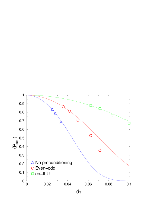
Figure 4: Acceptance rate vs. molecular dynamics step-size for three preconditioning schemes. Dashed lines are fits to Eqn. (39). All simulations are performed on $64\times 64$ lattices at $\beta=4.0,\kappa=0.2570$

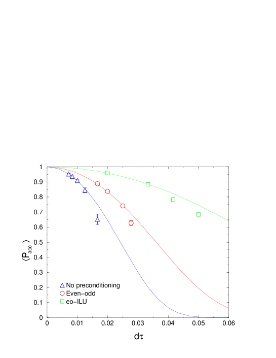
Figure 5: Acceptance rate vs. molecular dynamics step-size for three preconditioning schemes. Dashed lines are fits to Eqn. (39). All simulations are performed on $64\times 64$ lattices at $\beta=4.0,\kappa=0.2605$

The dependence of the acceptance probability on step-size for the two fermion masses are presented in Figs. 4 and 5. In these figures, fits to the expected small-step-size behaviour of the acceptance probability [9] are included,

$$\langle{\cal P}_{\rm acc}\rangle=\mbox{erfc }\left(\frac{d\tau}{\tau_{0}}\right)^{2},$$ (39)

where $\tau_{0}$ is a fit parameter and determines the characteristic scale of the equations of motion. $\tau_{0}$ presents a reliable estimate of the algorithm efficiencies, assuming the autocorrelations along the Markov chains for the different preconditionings are the same at a fixed Metropolis acceptance. While these autocorrelations have not been studied in detail, this criterion does appear to hold approximately. Eqn. (39) models the expected acceptance rate only in the limit $d\tau\rightarrow 0$. The fit gives an unacceptable $\chi^{2}$ once the acceptance rate falls below approximately 80%. At the lighter fermion mass $(\kappa=0.2605)$ the acceptance rate tended to break down rather suddenly as $d\tau$ was increased. The UKQCD collaboration [10] studied this phenomena in detail, and concludes that the leap-frog integrator becomes unstable at a critical value of $d\tau$, which decreases as the light quark mass is reduced. To determine $\tau_{0}$ from a fit, the number of data points included was increased (starting with the smallest $d\tau$) until $\chi^{2}/N_{\rm df}>1.5$. These fits are summarised in Table 4, along with the masses of the lightest mesons. Table 4 also includes the ratio of the characteristic molecular-dynamics time-scale of unpreconditioned HMC and the even-odd and eo-ILU schemes. For both values of the hopping parameter, the eo-ILU algorithm characteristic time is larger than standard HMC by a factor of about three and the even-odd method by about two. No significant mass dependence on this improvement is seen, although only two fermion masses were simulated.

$\beta=4.0,\;\kappa=0.2570$     $(am_{P}=0.210\pm 0.003)$
Preconditioning	$n_{\rm fit}$	$\chi^{2}/N_{\rm df}$	$\tau_{0}$	Improvement
none	2	1.00	0.0643(9)	—
eo	2	0.16	0.102(1)	1.59(3)
eo-ILU (B)	3	0.26	0.189(2)	2.94(5)
$\beta=4.0,\;\kappa=0.2605$     $(am_{P}=0.124\pm 0.005)$
Preconditioning	$n_{\rm fit}$	$\chi^{2}/N_{\rm df}$	$\tau_{0}$	Improvement
none	4	0.26	0.0351(6)	—
eo	3	0.23	0.0522(6)	1.48(3)
eo-ILU (B)	2	0.11	0.104(2)	2.96(8)

Table 4: Fits to Eqn. (39) at two $\kappa$ values for three HMC algorithms with no preconditioning, one step (even-odd) and two step (eo-ILU) preconditioning. $n_{\rm fit}$ indicates the number of points (starting from the lowest $d\tau$ data) that could be included in the fit before an unacceptably high $\chi^{2}/N_{\rm df}$ was found.

4 Discussion: further implementations

The preconditioned pseudofermion method, tested in the Schwinger model, can be applied directly in simulations of 4d gauge theories, such as QCD. As present, these computationally demanding calculations are being performed on large parallel computers. In Sec. 3, some correlation was seen between the performance of the preconditioned HMC algorithm and the condition number of the hermitian fermion matrix, $Q$. Finding the optimal site ordering is then reduced to minimising this condition number and a direct comparison of HMC performance from costly simulations can be avoided. Only a small set of orderings was tested in the two-dimensional study; the benefits of a given ordering will be dependent on the precise properties of the matrix in question and will differ in two and four dimensions.

These simulations also demonstrated that a significant enhancement in the performance of the HMC algorithm was found by using a two-step (eo-ILU) preconditioning of the pseudofermions. A highly efficient ordering for increasing the acceptance of the Metropolis test is a local one; ie. matrix operations still involve only a small neighbourhood (out to two hops) around each site and do not require global lattice sweeps for their operation. This means these preconditionings can be applied to simulations on parallel computers, as many processors can be working on independent portions of the local eo-ILU matrix-vector operation. The four-dimensional lattice would required sixteen indices to cover the orderings of the even-odd matrix and it is unclear whether this would lead to prohibitively expensive or complex communications on parallel computers. A direct test seems the only way to assess this. Sec. 3 determined that the acceptance rate is not critically dependent on the ordering and a better scheme for efficient parallelism could be found.

Ref. [11] demonstrated that the Sheikholeslami-Wohlert (SW) action can be simulated using even-odd preconditioned HMC. As with the Wilson matrix, the even-odd SW matrix can be ILU preconditioned again, leading to an eo-ILU scheme with a possible faster inverter performance and a larger useful molecular-dynamics step-size. Many large-scale dynamical quark simulations (eg. CP-PACS, UKQCD; see Ref. [12] for a review) use the SW fermion formulation. Lexicographic preconditioning has also been applied to more complex fermion matrices [13], and can be extended to highly improved actions with interactions beyond nearest neighbours, such as the Symanzik-improved $D234$ action [14] and fixed point actions [15, 16]. This work suggests HMC simulations of these fermion actions can be accelerated, even though the standard even-odd decomposition does not decouple even and odd sub-lattices. Note also that other dynamical fermion methods, such as the “Kentucky algorithm” [17] may also be enhanced by similar ILU or eo-ILU preconditioning.

As a final remark here, it is worth examining the hopping parameter expansion of the inverse preconditioned matrices. The original Wilson matrix inverse has a term at ${\cal O}(\kappa)$ while after any ILU preconditioning, the leading term appears at ${\cal O}(\kappa^{2})$. With the two-step eo-ILU preconditioning, the lowest order term is now ${\cal O}(\kappa^{4})$.

5 Conclusions

In this paper, ILU matrix preconditioning has been applied directly to the pseudofermion action of the hybrid Monte Carlo algorithm. The optimal ordering scheme for a single level of preconditioning in the pseudofermion action are local, like the simple even-odd checkerboard, while for inverting the fermion matrix a global-lexicographic ordering is best. The performance of the HMC algorithm was seen to depend weakly on the ordering, but to correlate with the condition number of the fermion matrix, while inversion performance has a more complex behaviour and is influenced strongly by the site indexing.

A two-level scheme was then introduced, in which the even-odd fermion matrix on a single sub-lattice was subsequently ILU preconditioned (eo-ILU). The global lexicographic ordering for this scheme was proposed in Section 4 of Ref. [4]. In direct analogy, the optimal ordering on the sub-lattice for inversion was found to be a global lexicographic scheme, while the HMC algorithm performed best with a more local, “four-flavour” decomposition. This optimal two-level scheme was found to improve the performance of the HMC algorithm by a factor of two over even-odd pseudofermions and a factor of three relative to the unmodified HMC method.

References

- [1] S. Duane, A. D. Kennedy, B. J. Pendleton and D. Roweth, Phys. Lett. B195, 216 (1987).
- [2] S. Fischer, A. Frommer, U. Glassner, T. Lippert, G. Ritzenhofer and K. Schilling, Comput. Phys. Commun. 98, 20 (1996) [hep-lat/9602019].
- [3] R. Gupta, A. Patel, C. F. Baillie, G. Guralnik, G. W. Kilcup and S. R. Sharpe, Phys. Rev. D40 (1989) 2072.
- [4] P. de Forcrand and T. Takaishi, Nucl. Phys. Proc. Suppl. 53 (1997) 968 [hep-lat/9608093].
- [5] Y. Oyanagi, Comput. Phys. Commun. 42, 333 (1986).
- [6] T. Lippert et al. [SESAM Collaboration], Nucl. Phys. Proc. Suppl. 63, 946 (1998) [hep-lat/9712020].
- [7] S. Eisenstat. J. Sci. Stat. Comput. 2 1 (1981).
- [8] J. C. Sexton and D. H. Weingarten, Nucl. Phys. B380, 665 (1992).
- [9] S. Gupta, A. Irback, F. Karsch and B. Petersson, Phys. Lett. B242 (1990) 437.
- [10] B. Joo, B. Pendleton, A. D. Kennedy, A. C. Irving, J. C. Sexton, S. M. Pickles and S. P. Booth [UKQCD Collaboration], hep-lat/0005023.
- [11] K. Jansen and C. Liu, Comput. Phys. Commun. 99 (1997) 221 [hep-lat/9603008].
- [12] R. D. Mawhinney, Nucl. Phys. Proc. Suppl. 83-84 (2000) 57 [hep-lat/0001032].
- [13] W. Bietenholz, N. Eicker, A. Frommer, T. Lippert, B. Medeke, K. Schilling and G. Weuffen, Comput. Phys. Commun. 119, 1 (1999) [hep-lat/9807013].
- [14] M. Alford, T. R. Klassen and G. P. Lepage, Phys. Rev. D58 (1998) 034503 [hep-lat/9712005].
- [15] W. Bietenholz and U. J. Wiese, Nucl. Phys. B464 (1996) 319 [hep-lat/9510026].
- [16] T. DeGrand [MILC Collaboration], Phys. Rev. D58 (1998) 094503 [hep-lat/9802012].
- [17] L. Lin, K. F. Liu and J. Sloan, Phys. Rev. D61, 074505 (2000) [hep-lat/9905033].