The Gribov Ambiguity for Maximal Abelian and Center Gauges in SU(2) Lattice Gauge Theory

Abstract

We present results for the fundamental string tension in SU(2) lattice gauge theory after projection to maximal abelian and direct maximal center gauges. We generate 20 Gribov copies/configuration. Abelian and center projected string tensions slowly decrease as higher values of the gauge functionals are reached.

The suggestion that a clearer view of confinement could be attained after gauge-fixing was first made by ’t Hooft, who also introduced the maximal abelian gauge (MAG) [1]. For an $SU(2)$ gauge theory, this gauge attempts to suppress the ‘charged’ gauge fields $A_{\mu}^{1},A_{\mu}^{2}$, and maximize the ‘abelian’ field $A_{\mu}^{3}$. In the continuum this is done by finding the minimum over the group of gauge transformations of the functional

$$G^{c}_{mag}=\frac{1}{2}\sum_{\mu}\int\left((A^{1}_{\mu})^{2}+(A^{2}_{\mu})^{2}\right)d^{4}x.$$ (1)

Minimizing $G_{mag}^{c}$ is equivalent in the limit of small lattice spacing to maximizing the lattice functional

$$G_{mag}^{l}=\frac{1}{2N_{link}}\sum_{x,\mu}{\rm tr}\left[U^{\dagger}_{\mu}(x)\sigma_{3}U_{\mu}(x)\sigma_{3}\right],$$ (2)

where $N_{link}$ is the number of links on the lattice. The normalization is such that $G_{mag}^{l}$ would be unity if every link were abelian.

Another gauge which has been widely studied in $SU(2)$ lattice gauge theory is the direct maximal center gauge (DCG) [2], which seeks the maximum of the functional

$$G_{dcg}^{l}=\frac{1}{4N_{link}}\sum_{x,\mu}({\rm tr}\left[U_{\mu}(x)\right])^{2}.$$ (3)

$G_{dcg}^{l}$ is normalized so that it would be unity if every link were a member of the center $Z(2)$ of $SU(2)$.

1 Gribov Ambiguities

Both the maximal abelian and maximal center gauges are subject to the Gribov ambiguity. This means that on a given lattice configuration, the functionals $G^{l}_{mag}$ and $G^{l}_{dcg}$ have many local maxima. The numerical application of a gauge-fixing algorithm will eventually put the configuration in the near vicinity of some local maximum. If before the application of the gauge-fixing algorithm, a random gauge transformation is applied, then upon gauge-fixing, the configuration in general approaches a different local maximum. A large number of so-called ‘Gribov copies’ of the original configuration can be generated in this way. A gauge invariant quantity will of course take the same value on any one of these copies. However, if the gauge invariant quantity is estimated by using approximate or ‘projected’ links, the value obtained will depend on which Gribov copy is utilized.

For the MAG, the link can be factored as

$$U_{\mu}(x)=U_{\mu}^{u1}(x)\cdot U_{\mu}^{\perp}(x),$$ (4)

where the abelian link $U_{\mu}^{u1}$ is a diagonal matrix [3]. Abelian projection means approximating the full $SU(2)$ link $U_{\mu}$ by its abelian part, $U_{\mu}^{u1}$.

For the DCG, the link is factored as

$$U_{\mu}(x)=Z_{\mu}(x)\cdot U_{\mu}^{\prime}(x),$$ (5)

where $Z_{\mu}(x)={\rm sign}({\rm tr}[U_{\mu}(x)])$. Center projection means replacing the full $SU(2)$ link by its center part, $Z_{\mu}$.

Table 1: Functional and string tension values for MAG

	$N_{copy}$	$G_{mag}^{l}$	$\sigma_{U(1)}$	$\sigma_{mon}$
	1	0.7493(1)	0.038(1)	0.0329(2)
	10	0.7498(1)	0.034(1)	0.0299(4)
	20	0.7499(1)	0.033(1)	0.0292(5)

Table 2: Functional values, string tension, and P-vortex density for DCG

	$N_{copy}$	$G_{dcg}^{l}$	$\sigma_{Z(2)}$	$\rho_{Z(2)}$
	1	0.7917(1)	0.0395(5)	0.0315(1)
	10	0.7925(1)	0.0351(4)	0.0299(2)
	20	0.7927(1)	0.0343(4)	0.0296(1)

The effect of the Gribov ambiguity on the fundamental string tension has been studied for the maximal abelian gauge in [4, 5], and for the maximal center gauge in [6, 7, 8]. Since numerically finding the global maximum of the gauge functional is not really feasible, the procedure in practice has been to generate several copies/configuration, and determine how string tension estimates vary as higher values of the gauge functionals are reached. In all cases, it is found that higher values of the gauge functionals $G_{mag}^{l}$ and $G_{dcg}^{l}$ are correlated with lower estimates for the fundamental string tension.

2 Stopping Criteria

We have applied overrelaxation methods [9] to finding local maxima of the functionals $G_{mag}^{l}$ and $G_{dcg}^{l}$. The iteration of the algorithm is stopped when a certain criterion is met, implying that the configuration is exceedingly close to a local maximum. For the MAG, a local maximum of $G_{mag}^{l}$ implies that

$$X_{i}(x) \equiv \frac{1}{2}\left\{\sum_{\mu}{\rm tr}\left[\sigma_{i}U_{\mu}(x)\sigma_{3}U^{\dagger}_{\mu}(x)\right]\right.$$

$$\left.+\sum_{\mu}{\rm tr}\left[\sigma_{i}U^{\dagger}_{\mu}(x-\hat{\mu})\sigma_{3}U_{\mu}(x-\hat{\mu})\right]\right\}$$

$$=0,\;\;i=1,2.$$

Defining the quantity

$$R_{mag}=\frac{1}{N_{site}}\sum_{x}\sum_{i=1}^{2}\left[|X_{i}(x)|^{2}\right],$$ (6)

we demand that $R_{mag}\leq 10^{-10}$.

For the DCG, a local maximum of $G_{dcg}^{l}$ implies that

$$X_{i}(x) \equiv \frac{1}{4}\left\{\sum_{\mu}{\rm tr}\left[\sigma_{i}U_{\mu}(x)\right]\cdot{\rm tr}\left[U_{\mu}(x)\right]\right.$$

$$\left.-\sum_{\mu}{\rm tr}\left[\sigma_{i}U_{\mu}(x-\hat{\mu})\right]\cdot{\rm tr}\left[U_{\mu}(x-\hat{\mu})\right]\right\}$$

$$=0,\;\;i=1,2,3.$$

Defining the quantity

$$R_{dcg}=\frac{1}{N_{site}}\sum_{x}\sum_{i=1}^{3}\left[|X_{i}(x)|^{2}\right],$$ (7)

we demand that $R_{dcg}\leq 10^{-12}$.

3 Results

Our calculations used a $24^{4}$ lattice at $\beta=2.50$. The results presented here are for 30 widely separated configurations. We gathered 20 Gribov copies/configuration for both MAG and DCG, where each copy satisfied the conditions of the previous section. We measured three types of projected Wilson loops $W(R,T)$, for $R=2-8,T=2-10$. For the MAG we measured $U(1)$ and monopole Wilson loops. The monopole Wilson loops are calculated from the magnetic currents of monopoles. The magnetic current is found by locating edges of Dirac sheets [10, 3]. For the DCG, we measured $Z(2)$ Wilson loops, which can be expressed in terms of the number of P-vortices piercing the loop [2]. The density of P-vortices, which is the same as the density of negative $Z(2)$ plaquettes, was also monitored.

The variation of results with the number of Gribov copies was handled exactly as in [5]. All possible sets of size $N_{copy}\leq 20$ were formed for each configuration, and on each set the copy with highest gauge functional was chosen. Wilson loops were computed, averaged over the sets, then averaged over configurations. The resulting average Wilson loops, indexed by $N_{copy}$, were used to extract potentials $V(R)$, by fitting $-\ln(W(R,T))$ to a straight line in $T$. Finally, string tensions were obtained by a linear-plus-Coulomb fit to $V(R)$ over the range $R=2-8$.

The gauge functionals, string tension values, and P-vortex densities are tabulated in Tables 1 and 2. From the tables, it is seen that a quite small relative increase in the gauge functionals corresponds to a much larger relative decrease in the string tensions. Comparing Tables 1 and 2, it is interesting to note the tendency of the monopole string tension to lie close to the density of P-vortices.

Figure 1 shows the string tension estimates vs $N_{copy}$, along with the full $SU(2)$ string tension (0.350(4)) from [11]. As the plot makes clear, taking one copy/configuration overestimates the string tensions, by an amount well outside of error bars. The results for $\sigma_{U(1)}$ and $\sigma_{Z(2)}$ are much closer to the full $SU(2)$ value for $N_{copy}=20$ than they are for $N_{copy}=1$. However, despite the apparent flattening out of the data as $N_{copy}$ increases, a very gradual descent to much smaller string tensions could still occur for $N_{copy}\gg 20$. That this is what happens for $\sigma_{Z(2)}$ is suggested by the results of [7], which finds significantly lower values of $\sigma_{Z(2)}$ than we report here, as well as higher functional values.

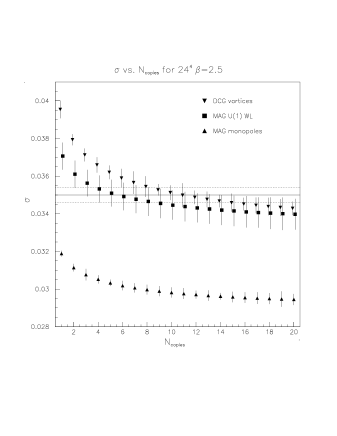
Figure 1: The fundamental string tension for MAG ($U(1)$ and monopoles) and DCG (P-vortices) vs. number of Gribov copies.

References

- [1] G. ’t Hooft, Nucl. Phys. B190 (1982) 455.
- [2] L. Del Debbio, M. Faber, J. Giedt, J. Greensite, and S. Olejnik, Phys. Rev. D58 (1998) 094501.
- [3] J. D. Stack, S. D. Neiman and R. J. Wensley, Phys. Rev. D50 (1994) 3399.
- [4] A. Hart and M. Teper, Phys. Rev. D55 (1997) 3756.
- [5] G. S. Bali, V. Bornyakov, M. Muller-Preussker, and K. Schilling, Phys. Rev. D54 (1996) 2863.
- [6] V. G. Bornyakov, D. A. Komoarov, A. I. Veselov, and M. I. Polikarpov, JETP Lett. 71 (2000) 231.
- [7] V. G. Bornyakov, D. A. Komarov, and M. I. Polikarpov, hep-lat/0009035.
- [8] R. Bertle, M. Faber, J. Greensite, and S. Olejnik, hep-lat/0010058.
- [9] J. Mandula and M. Ogilvie, Phys. Lett. B248 (1990) 156.
- [10] T. A. DeGrand and D. Toussaint, Phys. Rev. D22 (1980) 2478.
- [11] G. S. Bali, K. Schilling, and C. Schlichter, Phys. Rev. D51 (1995) 5165.