Matrix model formulation of four dimensional gravity

Abstract

The attempt of extending to higher dimensions the matrix model formulation of two-dimensional quantum gravity leads to the consideration of higher rank tensor models. We discuss how these models relate to four dimensional quantum gravity and the precise conditions allowing to associate a four-dimensional simplicial manifold to Feynman diagrams of a rank-four tensor model.

1 INTRODUCTION

The problem of constructing a quantum theory of gravity has been tackled with very different strategies. An attractive possibility is that of encoding all possible space-times as specific Feynman diagrams of a suitable field theory as it happens for the matrix model formulation of two-dimensional quantum gravity (see for example [1] and references therein). In the perturbative approach to the matrix model the resulting Feynman diagrams have vertices which correspond to two-simplices, and propagators which correspond to edge-pairings, so a diagram leads to a surface obtained by glueing triangles. Indeed one is brought to the search for theories having Feynman diagrams in which vertices can be identified with $n$-simplices, and propagators with glueings of codimension-1 faces. If this happens, each Feynman diagram can be identified as $n$-dimensional simplicial complex. We will discuss how the Feynman diagrams of an $n$-tensor model can be interpreted in this way. Moreover, we will discuss, in dimension four, the condition that must be fulfilled in order that the resulting space is a four manifold [3].

Figure 1: Feynman rules of a four-tensor generalized matrix model and the analogy of the vertex diagram with the four simplex.

2 GENERALIZED MATRIX MODELS

An n-tensor model is a generalization of the matrix model where the basic configuration variable is an n-tensor fulfilling the symmetry condition $\phi_{\alpha_{\tau(1)}\ldots\alpha_{\tau(n)}}=\Re[{\phi_{\alpha_{1}\ldots\alpha_{n}}}]+i\cdot{\rm sgn}(\tau)\cdot\Im[{\phi_{\alpha_{1}\ldots\alpha_{n}}}]$ (where $\tau\in{\hbox{\Got S}}_{n}$ and ${\rm sgn}(\tau)$ is the signature (also called parity) of $\tau$) and partition function

$$Z_{n}[N,\lambda]=\int[d\phi]\;\exp\Bigg{[}-\frac{1}{2}\sum_{\mathbf{\alpha}}|\phi_{\mathbf{\alpha}}|^{2}\qquad$$ (1)

$$\quad+\frac{\lambda}{n+1}\!\sum_{{\mathbf{\alpha}}^{\scriptscriptstyle(\!0\!)}\ldots{\mathbf{\alpha}}^{\scriptscriptstyle(\!n\!)}}\!V^{{\mathbf{\alpha}}^{\scriptscriptstyle(\!0\!)}\ldots{\mathbf{\alpha}}^{\scriptscriptstyle(\!n\!)}}\cdot\phi_{{\mathbf{\alpha}}^{\scriptscriptstyle(\!0\!)}}\cdot\ldots\cdot\phi_{{\mathbf{\alpha}}^{\scriptscriptstyle(\!n\!)}}\Bigg{]}$$

where $V^{{\mathbf{\alpha}}^{\scriptscriptstyle(\!0\!)}\ldots{\mathbf{\alpha}}^{\scriptscriptstyle(\!n\!)}}$ is a given vertex function and multi-indices ${\mathbf{\alpha}}=(\alpha_{1}\ldots\alpha_{n})$) are used. Its Feynman diagram expansion is

$$Z_{n} [N,\lambda]=\sum_{k}\sum_{\sigma\in{\hbox{\Got S}}_{\{0,\ldots,kn+k-1\}}}$$ (2)

$$\frac{1}{k!}\frac{\lambda^{k}}{(n+1)^{k}}\frac{(1/2)^{k(n+1)/2}}{(k(n+1)/2)!}\ \times$$

$$\times V^{{\mathbf{\alpha}}^{\scriptscriptstyle(\!0\!)}\ldots{\mathbf{\alpha}}^{\scriptscriptstyle(\!n\!)}}\cdot\ldots\cdot V^{{\mathbf{\alpha}}^{\scriptscriptstyle(\!kn+k-n-1\!)}\ldots{\mathbf{\alpha}}^{\scriptscriptstyle(\!kn+k-1\!)}}\ \times$$

$$\times G_{{\mathbf{\alpha}}^{\scriptscriptstyle(\!\sigma(0)\!)}{\mathbf{\alpha}}^{\scriptscriptstyle(\!\sigma(1)\!)}}\cdot\ldots\cdot G_{{\mathbf{\alpha}}^{\scriptscriptstyle(\!\sigma(kn+k-2)\!)}{\mathbf{\alpha}}^{\scriptscriptstyle(\!\sigma(kn+k-1)\!)}}$$

and the propagator is given by:

$$G_{\alpha_{1}\ldots\alpha_{n};\beta_{1}\ldots\beta_{n}}=\frac{2}{n!}\!\!\!\!\sum_{\begin{array}[]{c}\scriptstyle\tau\in{\hbox{\Got S}}_{n}\\[-2.84526pt] \scriptstyle{\rm sgn}(\tau)=-1\end{array}}\!\!\!\!\!\!G_{\alpha_{1}\ldots\alpha_{n};\beta_{1}\ldots\beta_{n}}^{\scriptscriptstyle(\!\tau\!)},$$ (3)

where $G_{\alpha_{1}\ldots\alpha_{n};\beta_{1}\ldots\beta_{n}}^{\scriptscriptstyle(\!\tau\!)}=\delta_{\alpha_{\tau(1)}\beta_{1}}\ldots\delta_{\alpha_{\tau(n)}\beta_{n}}$. It is straight-forward to encode the Feynman diagram expansion (2) in terms of $(n+1)$-valent graphs as follows. We associate tensor expressions to vertices and edges of a graph, according to the following rules:

$$G^{\scriptscriptstyle(\!\tau\!)}_{{\mathbf{\alpha}}^{\scriptscriptstyle(\!j\!)}{\mathbf{\alpha}}^{\scriptscriptstyle(\!i\!)}} \Rightarrow\begin{array}[]{c}\begin{picture}(70.0,35.0)\put(0.0,0.0){\makebox(10.0,10.0)[]{${\scriptscriptstyle(\!j\!)}$}} \put(20.0,10.0){\oval(30.0,30.0)[tl]} \put(20.0,25.0){\vector(1,0){30.0}} \put(30.0,27.0){\makebox(10.0,10.0)[]{$\sigma$}} \put(50.0,10.0){\oval(30.0,30.0)[tr]} \put(60.0,0.0){\makebox(10.0,10.0)[]{${\scriptscriptstyle(\!i\!)}$}} \end{picture}\end{array}$$ (5)

$$V^{{\mathbf{\alpha}}^{\scriptscriptstyle(\!i_{0}\!)}\ldots{\mathbf{\alpha}}^{\scriptscriptstyle(\!i_{n}\!)}} \Rightarrow\begin{array}[]{c}\begin{picture}(80.0,35.0)\put(40.0,15.0){\oval(70.0,30.0)[b]} \put(40.0,15.0){\oval(40.0,30.0)[b]} \put(40.0,0.0){\circle*{3.0}} \put(35.0,10.0){\makebox(10.0,10.0)[]{$\ldots$}} \put(5.0,7.0){\makebox(10.0,10.0)[]{$\scriptstyle 0$}} \put(20.0,7.0){\makebox(10.0,10.0)[]{$\scriptstyle 1$}} \put(75.0,7.0){\makebox(10.0,10.0)[]{$\scriptstyle n$}} \put(0.0,20.0){\makebox(10.0,10.0)[]{${\scriptscriptstyle(\!i_{0}\!)}$}} \put(15.0,20.0){\makebox(10.0,10.0)[]{${\scriptscriptstyle(\!i_{1}\!)}$}} \put(70.0,20.0){\makebox(10.0,10.0)[]{${\scriptscriptstyle(\!i_{n}\!)}$}} \end{picture}\end{array}$$ (7)

where $\tau=\sigma\circ(1\;n)$ and $\sigma$ is now an odd permutation. We call the graphs $G\in\textsf{FG}_{n}^{+}$ obtained using this procedure oriented fat $n$-graphs.

Using the definition just given we can rewrite (2) as a sum over all oriented fat $n$-graphs. Denoting by $\nu_{0}(G)$ and $\nu_{1}(G)$ the numbers of vertices and edges of a fat graph $G$, we have

$$Z_{n}[N,\lambda] =1+\!\!\sum_{G\in\textsf{FG}_{n}^{+}}w_{n}(G)\cdot\lambda^{\nu_{0}(G)}\cdot[[G]],$$ (8)

$$w_{n}(G) =\frac{\mu(G)}{\nu_{0}(G)!\cdot(n+1)^{\nu_{0}(G)}\cdot(n!)^{\nu_{1}(G)}},$$

where $\mu(G)$ is the number of the inequivalent ways of labeling the vertices of $G$ with $\nu_{0}(G)$ symbols and $[[G]]$ (the weight factor) denote the sum over all the possible values of the multi-indices ${\mathbf{\alpha}}^{\scriptscriptstyle(\!i\!)}$ of the associated tensor expression.

3 ASSOCIATED COMPLEXES

Consider a fat graph $G\in\textsf{FG}_{n}^{+}$ and associate to each vertex of $G$ an $n$-simplex $S(v)$ with labeled vertices $p_{i}(v)$ ($i=0,\ldots,n$) and the following object:

$$\!\!\!\!\!\!\!\!\!\!\!\!\begin{array}[]{c}\begin{picture}(250.0,50.0)\put(28.0,15.0){\makebox(0.0,0.0)[bl]{$\theta(p_{0}(v)$)}} \put(5.0,30.0){\line(1,0){40.0}} \put(5.0,35.0){\line(0,-1){5.0}} \put(0.0,37.0){\makebox(10.0,10.0)[]{$\scriptstyle i_{1}^{0}$}} \put(15.0,35.0){\line(0,-1){5.0}} \put(10.0,37.0){\makebox(10.0,10.0)[]{$\scriptstyle i_{2}^{0}$}} \put(25.0,37.0){\makebox(10.0,10.0)[]{$\ldots$}} \put(45.0,35.0){\line(0,-1){5.0}} \put(40.0,37.0){\makebox(10.0,10.0)[]{$\scriptstyle i_{n}^{0}$}} \put(98.0,15.0){\makebox(0.0,0.0)[bl]{$\theta(p_{1}(v)$)}} \put(75.0,30.0){\line(1,0){40.0}} \put(75.0,35.0){\line(0,-1){5.0}} \put(70.0,37.0){\makebox(10.0,10.0)[]{$\scriptstyle i_{1}^{1}$}} \put(85.0,35.0){\line(0,-1){5.0}} \put(80.0,37.0){\makebox(10.0,10.0)[]{$\scriptstyle i_{2}^{1}$}} \put(95.0,37.0){\makebox(10.0,10.0)[]{$\ldots$}} \put(115.0,35.0){\line(0,-1){5.0}} \put(110.0,37.0){\makebox(10.0,10.0)[]{$\scriptstyle i_{n}^{1}$}} \put(228.0,15.0){\makebox(0.0,0.0)[bl]{$\theta(p_{n}(v)$)}} \put(205.0,30.0){\line(1,0){40.0}} \put(205.0,35.0){\line(0,-1){5.0}} \put(200.0,37.0){\makebox(10.0,10.0)[]{$\scriptstyle i_{1}^{n}$}} \put(215.0,35.0){\line(0,-1){5.0}} \put(210.0,37.0){\makebox(10.0,10.0)[]{$\scriptstyle i_{2}^{n}$}} \put(225.0,37.0){\makebox(10.0,10.0)[]{$\ldots$}} \put(245.0,35.0){\line(0,-1){5.0}} \put(240.0,37.0){\makebox(10.0,10.0)[]{$\scriptstyle i_{n}^{n}$}} \put(125.0,0.0){\circle*{4.0}} \put(125.0,30.0){\oval(200.0,60.0)[b]} \put(125.0,30.0){\oval(60.0,60.0)[b]} \put(125.0,30.0){\oval(100.0,60.0)[br]} \put(160.0,20.0){$\cdots$} \end{picture}\end{array}$$ (10)

where $\theta(p_{i}(v))$ represents the face opposite to $p_{i}(v)$ and the sequence $(i_{1}^{k},i_{2}^{k},\cdots,i_{n}^{k})$ depends on whether $n\cdot k$ is even or odd. If $n\cdot k$ is even then the sequence is $(k-1,k-2,\cdots,k-n)$, with indices meant modulo $n+1$, while if $n\cdot k$ is odd then the sequence is $(k+1,k+2,\cdots,k+n)$, with indices again modulo $n+1$. Now, each edge of $G$ determines a pairing (simplicial identification) between the $(n\!-\!1)$-faces associated to its ends. In fact an edge of $G$ can be pictured as follows:

$$\begin{array}[]{c}\begin{picture}(200.0,60.0)\put(25.0,5.0){\line(0,1){10.0}} \put(27.0,0.0){$\theta(p_{j_{0}}\!(v))$} \put(5.0,15.0){\line(1,0){40.0}} \put(5.0,20.0){\line(0,-1){5.0}} \put(0.0,22.0){\makebox(10.0,10.0)[]{$\scriptstyle j_{1}$}} \put(15.0,20.0){\line(0,-1){5.0}} \put(10.0,22.0){\makebox(10.0,10.0)[]{$\scriptstyle j_{2}$}} \put(25.0,22.0){\makebox(10.0,10.0)[]{$\ldots$}} \put(45.0,20.0){\line(0,-1){5.0}} \put(40.0,22.0){\makebox(10.0,10.0)[]{$\scriptstyle j_{n}$}} \put(40.0,35.0){\oval(30.0,30.0)[tl]} \put(40.0,50.0){\vector(1,0){70.0}} \put(70.0,52.0){\makebox(10.0,10.0)[]{$\sigma$}} \put(110.0,35.0){\oval(30.0,30.0)[tr]} \put(125.0,5.0){\line(0,1){10.0}} \put(127.0,0.0){$\theta(p_{i_{0}}\!(w))$} \put(105.0,15.0){\line(1,0){40.0}} \put(105.0,20.0){\line(0,-1){5.0}} \put(100.0,22.0){\makebox(10.0,10.0)[]{$\scriptstyle i_{1}$}} \put(115.0,20.0){\line(0,-1){5.0}} \put(110.0,22.0){\makebox(10.0,10.0)[]{$\scriptstyle i_{2}$}} \put(125.0,22.0){\makebox(10.0,10.0)[]{$\ldots$}} \put(145.0,20.0){\line(0,-1){5.0}} \put(140.0,22.0){\makebox(10.0,10.0)[]{$\scriptstyle i_{n}$}} \end{picture}\end{array}$$ (12)

and it defines the map from $\theta(p_{i_{0}}(v))$ to $\theta(p_{j_{0}}(w))$ which maps $p_{i_{k}}(v)$ to $p_{j_{\tau(k)}}(w)$ where $\tau=\sigma\circ(1\;n)$. Summing up, we have associated to $G\in\textsf{FG}_{n}^{+}$ a set ${\cal S}$ of $n$-simplices and a face-pairing ${\cal P}$ on this set. The result is then a triangulated complex $X={\cal S}/{\cal P}$ made up of glued $n$-simplices. This is nothing else then the straightforward generalization to arbitrary dimension of the rule used in the case of the standard matrix model. In fact, these rules associate the three basic order two diagram of the matrix model:

to the torus (D3) and to the two inequivalent simplicial decomposition of the sphere (D1 and D2).

Taking Fig. 1 as model, one can rather easily transform (LABEL:rules1) and (12) into rules which allow to associate to a fat graph $G$ a pattern of circuits on the graph. If there are $\nu_{2}(G)$ of these circuits and we attach $\nu_{2}(G)$ discs $D^{2}$ to $G$ along them, we get a two polyhedron that is the 2-skeleton of the cellularization dual to the triangulation defined by the graph. We can then interpret the fat graph as a way of describing the dual 2-skeleton of a triangulation. In particular, this dual 2-skeleton determines the triangulation itself. This consideration implies that a model was Feynman diagrams can be coded in terms of fat graph can be seen as spin-foam models [8] and viceversa. Moreover, if the vertex function, as in the case of the 4-tensor model defined by

$$Z_{4}[N, \lambda]=\!\!\int\![d\phi]\exp\Bigg{[}\!-\frac{1}{2}\!\!\sum_{\alpha_{1},\ldots,\alpha_{4}}\!\!|\phi_{\alpha_{1}\alpha_{2}\alpha_{3}\alpha_{4}}|^{2}$$

$$+\frac{\lambda}{5}\sum_{\alpha_{1},\ldots,\alpha_{10}}\phi_{\alpha_{1}\alpha_{2}\alpha_{3}\alpha_{4}}\phi_{\alpha_{4}\alpha_{5}\alpha_{6}\alpha_{7}}\phi_{\alpha_{7}\alpha_{3}\alpha_{8}\alpha_{9}}$$

$$\quad\quad\quad\quad\quad\phi_{\alpha_{9}\alpha_{6}\alpha_{2}\alpha_{10}}\phi_{\alpha_{10}\alpha_{8}\alpha_{5}\alpha_{1}}\Bigg{]}\ \ ,$$ (13)

is modeled on rule (LABEL:rules1), then, in the evaluation of the weight factor $[[G]]$ of (8), there are exactly $\nu_{2}(G)$ traces. Indeed

$$Z_{n} [N,\lambda]=1+\!\!\sum_{G\in\textsf{FG}_{n}^{+}}w_{n}(G)\cdot\lambda^{\nu_{0}(G)}\cdot N^{\nu_{2}(G)}$$

$$=1+\!\!\sum_{G\in\textsf{FG}_{n}^{+}}w_{n}(G){\rm e}^{-k_{n}\nu_{n}({\cal T})+h_{n-2}\nu_{n-2}({\cal T})}$$

where, in the last line, we have introduced the standard dynamical triangulation constant and ${\cal T}$ is the simplicial complex associated to the fat graph $G$.

4 MANIFOLD CONDITIONS

In the previous section we discussed how to each fat graph is naturally associated a simplicial complex obtained by orientation preserving gluing of simplices. We have associated to each $G\in\textsf{FG}_{n}^{+}$ the topological (triangulated) space X. There is indeed a very important question to answer: is the space $X$ a manifold? That is, it is true that each point of $X$ has a closed neighborhood topologically equivalent to the $n$-disk $D^{n}$? In dimensions two, three and four (the only ones for which a definite answer it is available) the manifold question become simpler if we consider the closed space with boundary $X^{\partial}$ construct glueing the polyhedrons (instead of $n$-simplices) obtained removing the open star of the original vertices (as in fig. 2).

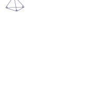
Figure 2: The basic building block in three-dimension. The shaded areas, after gluing, will become the boundary components of $X^{\partial}$

Then, $X$ is a manifold if and only if the boundary of $X^{\partial}$ is the disjoint union of $(n\!-\!1)$-spheres.

Clearly, there is nothing to check for all the points that lies on the interior of the simplices or on codimension 1 faces. Indeed, in dimension two, $X^{\partial}$ is always a manifold with boundary. Moreover, since the boundary components are always circle, $X$ is always a Manifold. In dimension three, one has to check the manifold conditions only on the points lying on the edges. It comes out that, since we are considering only orientation preserving gluing, that $X^{\partial}$ is always a three manifold with boundary.

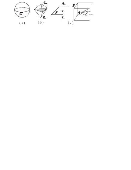
Figure 3: Links of the barycentres of a triangle (a) and an edge (b) in dimension four. The link of the midpoint of an edge is the double cone on the link in a cross-section (c). The triangle involved in the Surf condition is shaded.

In dimension four the manifold question for $X^{\partial}$ has a more elaborate answer. In this case, we have to check the manifold condition on the barycenters of triangles and edges. They generate conditions Cycl and Surf of [3], respectively. It is important to note that they are purely combinatorial conditions on the fat 4-graph. By lack of space we can not give here a complete description of these conditions and we refer the interested reader to [3]. They generate as follows. In PL-topology the concept of boundary of a closed neighborhood of a point $x$ is expressed as the link of the point $x$. We have that the manifold condition is indeed that the link of every points is homeomorphic to a 3-sphere. Now, we have that each 4-simplex contributes to the link of a point on a triangle or on an edges with the components showed in Fig. 3. The gluing instruction translate on gluing instruction for these components and the two conditions are the conditions that the objects obtained after gluing are 3-spheres.

5 GENERALIZED MODEL IN DIMENSION FOUR

Since in dimension four, not to all the fat graphs is associated a manifold, the $4$-tensor model cannot be used to define a viable theory of quantum gravity. We need a theory able to discriminate fat graphs to which is associated a manifold with respect to the other ones. This leads to consider generalization of this kind of model using fields over homogeneous (like Lie groups) spaces instead of $n$-tensors. The hope is that they are reach enough to make such discrimination. Example of theories of this kind are the ones discussed by Boulatov [5], Ooguri [6], and more recently by De Pietri et all. [2]. In dimension four one can use as basic variable a field $\phi(x_{1},\ldots,x_{4})$ over four copy of an homogeneous space $X$ over which is defined the action of a group $G$. It is possible to construct generalization of the 4-tensor model requiring that the field $\phi(x_{1},\ldots,x_{4})$ be real and invariant under any cyclic permutations of any three of its indices and using the action:

$$\begin{split}&S[\phi]=\frac{1}{2}\int\prod_{i=1}^{4}dx_{i}~{}\phi^{2}(x_{1},x_{2},x_{3},x_{4})\\[-2.84526pt] &+\frac{\lambda}{5!}\int\prod_{i=1}^{10}dx_{i}~{}~{}\phi(x_{1},x_{2},x_{3},x_{4})\phi(x_{4},x_{5},x_{6},x_{7})\\[-2.84526pt] &\phi(x_{7},x_{3},x_{8},x_{9})\phi(x_{9},x_{6},x_{2},x_{10})\phi(x_{10},x_{8},x_{5},x_{1}).\end{split}$$

In the case $X=G=SU(2)$ it is possible to show [6] that the Feynman diagram expansion of this theory is still given by (8) where now the weight factor associated to each fat graph $[[G]]=OCY[G]$ is the Ooguri-Crane-Yetter invariant construct on the dual two skeleton of the space of glued simplices $G$. In the same way, if $X=SO(4)/SO(3)$, $G=SO(4)$ the same procedure will give a weight factor $[[G]]=BC[G]$ is the Barrett-Crane [7] state sum associated to the space of glued simplices $G$ (see [2]).

Acknowledgements: This work is based on results obtained in collaboration with Laurent Freidel, Kiril Krasnov, Carlo Petronio and Carlo Rovelli.

References

• [1] J. Ambjorn, J. Jurkiewicz, Y. Watabiki, J. Math. Phys. 36, 6299 (1995).
• [2] R. De Pietri, L. Freidel, K. Krasnov and C. Rovelli, Nucl. Phys. B 574, 785 (2000); A. Perez and C. Rovelli, gr-qc/0006107; D. Oriti and R. M. Williams, gr-qc/0010031.
• [3] R. De Pietri and C. Petronio J. Math. Phys. 41, 6671 (2000).
• [4] G. Ponzano, T. Regge, in Spectroscopy and group theoretical methods in Physics, F. Bloch ed. (North-Holland, Amsterdam, 1968).
• [5] D. V. Boulatov, Mod. Phys. Lett. A7, 1629 (1992); Int. J. Mod. Phys. A8, 3139 (1993).
• [6] H. Ooguri, Mod. Phys. Lett. A7, 2799 (1992).
• [7] J. W. Barrett, L. Crane, J. Math. Phys. 39, 3296 (1998).
• [8] R. De Pietri, in Recent Developments in General Relativity, B. Casciaro, D. Fortunato, M. Francaviglia eds. (Springer-Verlag, Milano). gr-qc/9903076.