The Gluon Propagator without lattice Gribov copies

Abstract

We study the gluon propagator in quenched lattice QCD using the Laplacian gauge which is free of lattice Gribov copies. We compare our results with those obtained in the Landau gauge on the lattice, as well as with various approximate solutions of the Dyson Schwinger equations. We find a finite value $\sim(445\rm{MeV})^{-2}$ for the renormalized zero-momentum propagator (taking our renormalization point at $1.943$ GeV), and a pole mass $\sim 640\pm 140$ MeV.

PACS numbers: 11.15.Ha, 12.38.Gc, 12.38.Aw, 12.38.-t, 14.70.Dj

1 Introduction

Over the last twenty years, widely different conjectures have been proposed for the infrared behaviour of the gluon propagator. Although it is a gauge dependent quantity, it can be discussed in a given gauge. Even within the same gauge, the proposals for the infrared dependence differ drastically [1]. We mainly summarize here the results that are given in the literature within the Landau gauge, since that gauge is widely used in studies of Dyson Schwinger equations (DSE) as well as in lattice QCD. Early predictions were obtained by solving approximately the DSE. Mandelstam [2] obtained a solution of a set of truncated DSE equations with an infrared behaviour of the form $(q^{2})^{-2}$ for the gluon propagator. Such an infrared enhancement was shown, if obtained in any gauge, to lead to an area law for the Wilson loop [3] and thus to be sufficient for confinement. Infrared enhancement was assumed in various phenomenological studies [4] and corroborated by later studies of DSE with refined approximations [5]. A different perspective was taken by Gribov [6], who showed that avoiding gauge copies one would obtain a gluon propagator which vanishes in the infrared in the Landau and Coulomb gauges, of the form

$$D(q^{2})\sim\frac{q^{2}}{q^{4}+m^{4}}\quad.$$ (1.1)

An infrared suppressed behaviour was advocated by Stingl [7], and recently by others [8], as a possible solution to DSE. Following a procedure similar to that by Gribov, Zwanziger [9] gave arguments to show that, on the lattice, for any finite spacing in the limit of infinite volume, $D(q^{2}=0)=0$.

We will also consider in this work the parametrization deduced by Cornwall [10] using a resummation of Feynman graphs which leads to gauge-invariant amplitudes. The gluon propagator is obtained as a solution to this special set of DSE where the claim is that the only gauge dependence appears in the free part. Cornwall’s solution, in addition to fulfilling the Ward identities, allows a dynamical mass generation. Thus this formulation has the additional attractive feature that the gluon mass vanishes in the ultraviolet as required perturbatively. Since the self-energy obtained by Cornwall is claimed to be gauge-independent, we will use his model to fit the propagator both in the Landau and in the Laplacian gauge.

In contrast to all the approaches described above, lattice QCD provides a framework for the calculation of the gluon propagator starting directly from the QCD Lagrangian and can thus yield a conclusive result. Attempts to calculate the gluon propagator started more than ten years ago [11, 12] on rather small lattices. These early results could be interpreted in terms of a massive scalar propagator, but confirmed the expectation that a Lehmann-Källen representation is not applicable: positivity of the transfer matrix is lost after the non-local gauge fixing. Results on larger lattices were accounted for by assuming a positive anomalous dimension [13]. Recently, a detailed study of the gluon propagator on very large lattices [14] has been performed, which makes an impressive effort towards bringing under control errors due to the finite lattice spacing and to the finite lattice volume. However, up to now, all lattice studies have used a similar implementation of the Landau gauge on the lattice. Gauge-fixing is accomplished by using a local iterative procedure which identifies local stationarity, but in general fails to determine the global extremum. Which local extremum (“lattice Gribov copy”) is selected depends on the starting condition. These lattice Gribov copies cannot be eliminated. In this situation, their effect has repeatedly been claimed to be small [15]. As discussed in Section 3, we are not convinced by such claims. Results obtained so far will have a safer foundation if the effects of lattice Gribov copies are better understood.

In this work we address the problem of Gribov copies. We use a different gauge condition, which produces a smooth gauge field like the Landau gauge, but which specifies the gauge uniquely: no ambiguity arises due the lattice gauge fixing procedure. This is accomplished by using the Laplacian gauge [17]. The motivation and implementation of this gauge are given in section 3.

We calculate the gluon propagator in quenched QCD on lattices of sizes $8^{4},16^{4}$ and $16^{3}\times 32$ at $\beta=5.8$ and $6.0$, in an attempt to study its zero-temperature behaviour. Our procedure can be extended straightforwardly to finite temperature where the infrared behaviour of the propagator yields the chromo-electric and chromo-magnetic screening masses. The results that we obtain, within the Laplacian gauge, show the same ultraviolet behaviour as in Landau gauge. However, there are significant modifications in the infrared. In particular we find that the zero-momentum propagator is finite, obeys scaling, and becomes volume independent for large enough volumes. It should not however be used as a definition of the gluon mass, since the zero-momentum limit of the propagator is gauge dependent. It is simply a measure of the susceptibility of the gauge-fixed field $A_{\mu}$ in the Laplacian gauge. A quantity which instead can be shown to be gauge independent to all orders in perturbation theory is the pole mass of the transverse part $D(q^{2})$ of the propagator [18]. To determine this pole if it exists at all, an extrapolation to negative $q^{2}$ is necessary. We compare the inverse propagator $D^{-1}(q^{2})$ in the Laplacian and the Landau gauges. Using a variety of extrapolation ansätze, in particular a fit to Cornwall’s model [10] which describes the momentum dependence of our results rather well, we find that data in the Laplacian gauge give support for the existence of a pole at a mass of $\sim 640(140)$ MeV. Data at smaller momenta are needed to consolidate this result.

Section II introduces our notation; Section III motivates and describes our choice of the Laplacian gauge; Section IV presents our results. They are summarized in Section V.

2 Definition of the gluon propagator

The gluon propagator in the continuum is given by

$${\cal D}^{ab}_{\mu\nu}(q)=-i\int d^{4}x\langle 0|T[A^{a}_{\mu}(x)A^{b}_{\nu}(0)]|0\rangle e^{iq.x}$$ (2.2)

This tensor can be decomposed into a transverse and a longitudinal part:

$${\cal D}^{ab}_{\mu\nu}(q)=\biggl{(}\delta{\mu\nu}-\frac{q_{\mu}q\nu}{q^{2}}\biggr{)}\>\delta^{ab}\>D(q^{2})+\frac{q_{\mu}q_{\nu}}{q^{2}}\>\delta^{ab}\>\frac{F(q^{2})}{q^{2}}$$ (2.3)

For a covariant gauge $F(q^{2})$ reduces to a constant and corresponds to the gauge fixing parameter $\xi$ which in the Landau gauge is zero. Since we want to make a comparison with the recent results [14] obtained in the Landau gauge, we study the transverse scalar function $D(q^{2})$ which can be extracted from ${\cal D}^{ab}_{\mu\nu}(q)$:

$$D(q^{2})=\frac{1}{3}\biggl{\{}\sum_{\mu}\frac{1}{8}\sum_{a}{\cal D}^{aa}_{\mu\mu}(q)\biggr{\}}-\frac{1}{3}\frac{F(q^{2})}{q^{2}}\quad.$$ (2.4)

$F(q^{2})$ is determined by projecting the longitudinal part of ${\cal D}^{aa}_{\mu\nu}(q)$ using the symmetric tensor $q^{\mu}q^{\nu}$.

On the lattice the dimensionless gluon field can be defined by

$$A_{\mu}(x+\hat{\mu}/2)=\frac{1}{2ig_{0}}\biggl{\{}\left[U_{\mu}(x)-U^{\dagger}_{\mu}(x)\right]-\frac{1}{3}{\rm Tr}\left[U_{\mu}(x)-U^{\dagger}_{\mu}(x)\right]\biggr{\}}+{\cal O}(a^{3})$$ (2.5)

where $a$ is the lattice spacing. One may consider different definitions for the gluon field $A_{\mu}$, accurate to higher order in $a$. It has been found [19] that these different definitions give rise to modifications that can be absorbed in the multiplicative field renormalization constant.

The gluon propagator in momentum space is constructed by taking the discrete Fourier transform of $A_{\mu}$ for each colour component

$$A^{a}_{\mu}(q)=\sum_{x}e^{-iq.(x+\hat{\mu}/2)}A^{a}_{\mu}(x+\hat{\mu}/2)$$ (2.6)

where the discrete momentum $q=(q_{\mu},\mu=1,..,4)$ takes values

$$q_{\mu}=\frac{2\pi}{a{\rm L}_{\mu}}n_{\mu},\hskip 28.45274ptn_{\mu}=-(\frac{1}{2}{\rm L}_{\mu}-1),...,(\frac{1}{2}{\rm L}_{\mu})$$ (2.7)

and the momentum-space gluon propagator $D^{ab}_{\mu\nu}(q)$ is defined by

$${\rm V}~{}\delta(q-q^{\prime})D^{ab}_{\mu\nu}(q)=\langle A^{a}_{\mu}(q)A^{b}_{\nu}(-q^{\prime})\rangle\quad.$$ (2.8)

with $V$ the lattice volume. In the ultraviolet the gluon propagator is expected to behave like $1/q^{2}$. Since on the lattice the free massless propagator behaves as

$$D(q)=\frac{1}{\sum_{\mu}\left(\frac{2}{a}\>\>\sin\frac{q_{\mu}a}{2}\right)^{2}},$$ (2.9)

to reduce errors due to the finite lattice spacing we take as our momentum variable the usual

$$\hat{q}_{\mu}=\frac{2}{a}{\rm sin}\frac{q_{\mu}a}{2}$$ (2.10)

To relate the bare lattice propagator to the renormalized continuum propagator $D_{\rm R}(q;\mu)$ one needs the renormalization constant $Z_{3}(\mu,a)$:

$$a^{2}D(qa)=Z_{3}(\mu,a)D_{\rm R}(q;\mu)\quad.$$ (2.11)

Imposing a renormalization condition such as

$$D_{\rm R}(q)|_{q^{2}=\mu^{2}}=\frac{1}{\mu^{2}}$$ (2.12)

at a renormalization scale $\mu$ allows a determination of $Z_{3}(\mu,a)$. Connection to other continuum renormalization schemes can then be made.

3 Gauge fixing procedure

3.1 Motivation

The gluon propagator is normally considered in Landau gauge, $\partial_{\mu}A_{\mu}(x)=0~{}\forall x$. On the lattice, this condition becomes:

$$F(\Omega)\equiv\sum_{x,\mu}{\rm Re~{}Tr}~{}(\Omega(x)^{\dagger}U_{\mu}(x)\Omega(x+\hat{\mu}))~{}~{}~{}~{}~{}{\rm maximum}$$ (3.13)

The gauge-fixing functional $F$ has many local maxima. To specify the gauge uniquely, the gauge condition above refers to the global maximum. This defines the Fundamental Modular Region (FMR) Landau gauge. In practice however, the gauge transformation $\Omega$ is found by an iterative local maximization of $F$, which terminates when any local maximum has been reached. A different gauge condition is thus implemented, which one might call the random Landau gauge, and which depends on the details of the maximization procedure.

It is commonly believed that the effect of choosing a local maximum of (3.13) rather than the global maximum is small, so that the “random” Landau gauge is a good approximation to the FMR Landau gauge. The following argument is often presented to support this view. A given gauge configuration is gauge-fixed $n$ times, each time after performing a random gauge transformation; this procedure generates many gauge copies, each corresponding to the local maximum nearest to the random starting point along the gauge orbit. It is observed [20] that the difference between gluon propagators measured on copies corresponding to the largest and the smallest values of (3.13) is found to be statistically insignificant. A possible problem with this argument however is that the number $n$ of gauge copies considered in such comparisons (typically 30 or less) is extremely small compared to the total number of local extrema of (3.13): for simple entropic reasons, all copies considered miss the global maximum by similar amounts, and no reliable information can be extracted about the gluon propagator in the global maximum configuration. It is therefore possible, and we believe quite likely, that the “random” Landau gauge and the FMR Landau gauge are significantly different.

Further evidence for this situation has recently been provided in another gauge, the Direct Maximal Center (DMC) gauge [21]. Although the functional $F_{DMC}(\Omega)$ to be maximized differs from (3.13), a similar approach of local iterative maximization is taken, leading to the “random” DMC gauge, with similar problems. In this case however, it is also possible to converge to a large value $\tilde{F}_{L}$ of $F_{DMC}$ by starting from a Landau gauge copy (“Landau” DMC gauge). This value $\tilde{F}_{L}$ can then be compared with the values obtained from $n$ random starting points. One may fit the maximum value among $n$ copies, $\tilde{F}(n)$, by a reasonable ansatz like a series in $1/n$, and extrapolate to $n\rightarrow\infty$. It turns out that the extrapolated value falls well below $\tilde{F}_{L}$, which is itself below the global maximum [22]. Furthermore, the properties of the gauge-fixed field are qualitatively different between the “random” and the “Landau” DMC gauges: the former confines after center projection, while the latter does not [16].

Since in Landau gauge as in DMC gauge, the number of local maxima is expected to grow exponentially with the lattice volume, we expect a similar situation in Landau gauge, leading to large differences between the “random” (local maximum) and the FMR (global maximum) gauges. One might argue that this is not a problem, and that the local maximization of (3.13) implements in the thermodynamic limit a well-defined, but stochastic gauge condition. The relationship between that gauge condition and its perturbative version $\partial_{\mu}A_{\mu}(x)=0$ is unclear however. Therefore, one should consider the possible effects of selecting a local rather than the global maximum of (3.13) with a great deal of caution. This is the motivation for our study of the gluon propagator in a well-defined, unambiguous gauge.

3.2 $SU(3)$ Laplacian gauge fixing

In [17], Vink and Wiese proposed a simple method to fix the gauge unambiguously in $SU(N)$. It uses $N$ auxiliary Higgs fields, which are chosen as the $N$ lowest-lying eigenvectors $v^{(i)}$ of the covariant Laplacian. Under a local gauge transformation $\Omega(x)$, these eigenvectors transform covariantly: $v^{(i)}(x)\rightarrow\Omega(x)v^{(i)}(x)$. Therefore, the gauge can be fixed by requiring, at each space-time point $x$, $\{\Omega(x)v^{(i)}(x),i=1,..,N\}$ to have some predefined orientation in color space. Specifically, each eigenvector $v^{(i)}(x)$ has $N$ complex color components, so that the $N$ eigenvectors form a complex $N$ by $N$ matrix $M$. Ref.[17] projects this matrix onto $SU(N)$ by polar decomposition: $M=WP,W\in U(N),P=(M^{\dagger}M)^{1/2}$. The required gauge transformation is then $\Omega(x)=e^{i\alpha}W^{\dagger}$, where $\alpha=\frac{1}{N}{\rm arg}(\det W)$. $\Omega(x)$ rotates $M$ “parallel” to the identity ${\bf 1}_{N}$ at each space-time point. The gauge is unambiguously defined, except for these gauge configurations where some of the $N$ lowest eigenvalues are degenerate. Such configurations are genuine Gribov copies; they never occur in practice. This approach has been tested for $SU(2)$ and $U(1)$  [23] and it was shown to reduce to the Landau gauge in the continuum limit aside from exceptional configurations (e.g. an instanton background). Here, we use a slightly modified procedure which requires only $(N-1)$ eigenvectors (2 for $SU(3)$), as follows [24].

First, apply a gauge transformation $\Omega^{(1)}(x)$ which rotates $v^{(1)}(x)$ to $\left(\begin{array}[]{c}|v^{(1)}(x)|\\ 0\\ 0\end{array}\right)$. Five real components of the rotated $v^{(1)}(x)$ must vanish, which specifies five constraints. Therefore $\Omega^{(1)}(x)$ is not fully specified, but has $8-5=3$ degrees of freedom. Any satisfactory $\Omega^{(1)}$ can be used.

To completely fix the gauge, we use the second eigenvector $v^{(2)}$, already rotated by $\Omega^{(1)}$ to $\left(\begin{array}[]{c}v^{(2)}_{1}\\ v^{(2)}_{2}\\ v^{(2)}_{3}\end{array}\right)$. Three additional constraints are obtained by requiring $v^{(2)}$ to be rotated to $\left(\begin{array}[]{c}v^{(2)}_{1}\\ \sqrt{|v^{(2)}_{2}|^{2}+|v^{(2)}_{3}|^{2}}\\ 0\end{array}\right)$. This fixes the gauge completely and uniquely.

Note that the second rotation is in an $SU(2)$ subgroup, since it leaves $v^{(2)}_{1}$ untouched. This indicates how to generalize this construction to $SU(N)$: the first rotation fixes $(2N-1)$ constraints, which leaves $(N^{2}-1)-(2N-1)=((N-1)^{2}-1)$ degrees of freedom, forming a subgroup $SU(N-1)$. The next step reduces the gauge freedom to $SU(N-2)$, etc… down to $SU(2)$. It is easily seen that, in this recursive procedure, the matrix $M$ is reduced to upper triangular form (with real positive diagonal elements) by the rotation $\Omega(x)$. This is why the $N^{th}$ eigenvector needs not be computed: it is only transformed by a phase, which is separately determined by the requirement that $\Omega(x)\in SU(N)$. Our procedure can thus be viewed as a $QR$ decomposition of $M$. The gauge, which is globally well-defined (provided the $N$ eigenvalues are distinct), may be ill-defined on a sub-manifold of points $x$ where our recursive process breaks down. It can be seen that such local gauge defects occur at isolated points, where for $SU(3)$, $\sqrt{|v^{(2)}_{2}|^{2}+|v^{(2)}_{3}|^{2}}=0$. The correlation of these points with instantons is studied in [24].

The Laplacian gauge so defined has the great virtue of being unambiguous. Hence it is the appropriate tool to address our concern about the effect of local extrema of the usual Landau gauge. It also has strong similarities with Landau gauge: it is smooth, Lorentz-symmetric, and gauge-fixes a pure gauge lattice configuration (gauge-transformed from $U_{\mu}(x)={\bf 1}~{}\forall x,\mu$) back to $U={\bf 1}$. Nevertheless, it is a different gauge: its perturbative definition is under consideration [25]; it differs from Landau gauge most strongly where the magnitude of the eigenvectors $|v^{(1,2)}(x)|$ becomes small.

4 Results

Since most of the previous studies were performed in the Landau gauge, it is important to compare our Laplacian-gauge propagator with the Landau-gauge one. For this purpose, we have taken, for our analysis, lattice configurations available on the Gauge Connection database [27], which had already been gauge fixed to Landau gauge with the usual local Over-Relaxation method [28]. These are 200 configurations of a $16^{3}\times 32$ lattice, at $\beta=5.8$ and $6.0$ each.

The transverse gluon propagator is shown in Fig. 1 for the two gauges at $\beta=6.0$. As expected the ultraviolet behaviour is identical in the two gauges, whereas in the infrared, which is the region of interest, significant differences are visible. Since we use a different gauge, this should not come as a surprise. We show the usual quantity $\hat{q}^{2}D(q^{2})$. The Laplacian propagator is clearly not as large as the Landau propagator at low momenta.

The difference between Landau and Laplacian gauge can also be seen in the deviation of $F(q^{2})$ from zero. Whereas in Landau gauge we find that

$$\hat{q}^{\mu}\hat{q}^{\nu}{\cal D}^{aa}_{\mu\nu}\ll 1$$ (4.14)

as expected, in the Laplacian gauge $F(q^{2})$ is not small, and has a maximum at low momenta. The behaviour of $F(q^{2})$ is shown in Fig. 2 for $8^{4}$ and $16^{3}\times 32$ lattices at $\beta=6.0$. Since $F(q^{2}=0)$ can not be obtained by our projection, we only have one point, at the smallest momentum $2\pi/32$ on the larger lattice, to ascertain that $F(q^{2})$ really has a maximum and does not keep diverging as $q^{2}\rightarrow 0$. But since the data are systematically higher for the smaller lattice than for the larger one, it seems unlikely that increasing the lattice size further would bring the infrared data up and remove the maximum.

It is interesting to examine the volume dependence of the zero-momentum propagator ${\cal D}(0)\equiv\frac{1}{4}\sum\nolimits_{\mu\mu}\sum\nolimits_{\alpha}{\cal D}_{\mu\mu}^{\alpha\alpha}(q^{2}=0)$. We note that in order to determine the transverse part of the propagator at zero-momentum, $D(0)$, one must subtract from ${\cal D}(q^{2})$ $F(q^{2})/q^{2}|_{q^{2}=0}$, which we can only obtain as ${\rm lim}_{q^{2}\rightarrow 0}F(q^{2})/q^{2}$.

FIG. 1.: Comparison of the transverse gluon propagator times $q^{2}$ in Landau and Laplacian gauge on a $16^{3}\times 32$ lattice at $\beta=6.0$.

FIG. 2.: $F(q^{2})$ as a function of $|\hat{q}|$ in lattice units after applying the cylindrical cut in momentum.

FIG. 3.: The Renormalized zero-momentum propagator ${\cal D}(0)\equiv\frac{1}{4}\sum\nolimits_{\mu\mu}\sum\nolimits_{\alpha}\frac{1}{8}{\cal D}_{\mu\mu}^{\alpha\alpha}(q^{2}=0)$ versus volume in physical units. The dashed line is a fit to the form $a\exp{(-V/V_{0})}+c$.

¿From Fig. 2 it can be seen that to extract the limit of $F(q^{2})/q^{2}$ as $q^{2}\rightarrow 0$ reliably, one needs more data in the infrared. Therefore, with the volumes at our disposal we can only examine the zero-momentum limit ${\cal D}(0)$ of the full propagator. In the Landau gauge, Zwanziger has argued that $D(0)={\cal D}(0)$ should vanish in the infinite lattice volume limit [9]. A recent lattice study in $SU(2)$ at finite temperature [20] seems indeed to indicate such a behaviour. With the data on our present volumes the needed subtraction in the Laplacian gauge cannot be reliably performed, and thus we cannot extract $D(0)$. What we find is that ${\cal D}(0)$, the zero-momentum propagator, is finite and volume independent for large enough volumes. The volume dependence and scaling of the renormalized zero-momentum propagator in physical units is displayed in Fig. 3 where we collected results from $\beta=5.8,6.0,6.2$ and $6.5$. To obtain the renormalized propagator we impose the renormalization condition given in eq. (2.12) where we choose the renormalization point to be $\mu=a^{-1}$ for $\beta=6.0$ i.e. $\mu=1.943$ GeV. This determines $Z_{3}(\mu,a_{\beta=6.0})\approx 2.312$. We then use eq. (2.11) to find the ratio of the factors $Z3$ for different $\beta$ values at the same physical momentum $q$, e.g. for $\beta=5.8$ at $q=\mu$ we have:

$$\frac{Z_{3}(\mu,a_{\beta=5.8})}{Z_{3}(\mu,a_{\beta=6.0})} = \frac{a_{\beta=5.8}^{2}D(qa_{\beta=5.8})}{a_{\beta=6.0}^{2}D(qa_{\beta=6.0})}$$ (4.15)

$$= 0.97(4)$$ (4.16)

In this way we obtain the renormalization factors at all $\beta$ values. For $\beta=6.2$ and $\beta=6.5$ we find 1.04(4) and 1.07(6) respectively as compared to the value at $\beta=6.0$. We also obtained consistent results by fitting our data in the ultraviolet regime using the asymptotic one-loop result for $D_{R}\sim Z/q^{2}(1/2\ln(q^{2}/\Lambda^{2}))^{-d_{D}}$, with $d_{D}=13/22$ as in the Landau gauge since in this regime the results in the Laplacian and Landau gauges are the same. As can be seen from Fig. 3 the renormalized ${\cal D}(0)$ displays reasonable scaling, and appears quite volume-independent for volumes larger than $\sim 1/2$ fm⁴. We find a value of ${\cal D}(0)=5.020(16)$ GeV^-2, or ${\cal D}(0)^{-1/2}=445(3)$ MeV, corresponding to a length scale of $\sim 0.5$ fm. Since the zero-momentum propagator measures the susceptibility of the $A_{\mu}^{a}$ field, the length associated with it determines the domain over which the gluon field remains correlated in the Laplacian gauge. If the lattice dimensions become of the order of this characteristic length, then one expects finite size effects to become appreciable. This is indeed what is observed, as shown in Fig.3, with an approximate volume dependence of $exp(-V/V_{0})$ with $V$ the lattice volume and $V_{0}\sim{\cal D}(0)^{2}$.

On the lattice, the Lorentz symmetry is only approximately restored. Lattice artifacts cause some dependence of $D(q)$ on the orientation of the vector $q$ rather than just on $q^{2}$. To minimize these discretization effects, we filter our data by making a cylindrical cut in momentum along a reference direction $\hat{n}=\frac{1}{2}(1,1,1,1)$, in the same manner as in Ref. [14]. Namely, we only consider momenta obeying the criterion $|\Delta\hat{q}|<2\pi/L_{s}$, where $L_{s}$ is the number of sites in the spatial direction, and $\Delta\hat{q}$ is the momentum transverse to $\hat{n}$ ($\Delta\hat{q}=\hat{q}-\hat{q}.\hat{n}~{}\hat{n}$). Using these filtered data which allow a direct comparison with [14], we examine the various proposals discussed in the Introduction for the infrared behaviour of the propagator. We find that Gribov type parametrizations [6, 7] as well as infrared enhancement of the type $(q^{2})^{-2}$ [2, 4, 5] are excluded [29]. The ansatz of Marenzoni et al. [13],

$$D(q^{2})=\frac{Z}{(q^{2})^{1+\alpha}+M^{2}}\quad,$$ (4.17)

with a non-perturbative anomalous dimension $\alpha$, gives a better description of the lattice data than the aforementioned parametrizations, but, as seen in Fig. 4, underestimates the peak of the propagator. On the other hand, Cornwall [10] allows for a dynamically generated gluon mass which vanishes at large momentum in accord with perturbation theory. Using a special set of DSE referred to as a gauge invariant “pinch technique”, he obtains the following solution for the gluon propagator

$$D(q^{2})=Z\>\biggl{[}\left(q^{2}+M^{2}(q^{2})\right){\rm ln}\frac{q^{2}+4M^{2}(q^{2})}{\Lambda^{2}}\biggr{]}^{-1}$$

with

$$M(q^{2})=M\left\{\frac{{\rm ln}\left[(q^{2}+4M^{2})/\Lambda^{2}\right]}{{\rm ln}\left[4M^{2}/\Lambda^{2}\right]}\right\}^{-6/11}$$ (4.18)

FIG. 4.: The gluon propagator $D(q^{2})$ multiplied by $\hat{q}^{2}$ on the $16^{3}\times 32$ lattice at $\beta=6.0$. The dashed-dotted line shows the fit to the model by Marenzoni et al. eq.(4.17), the solid line to Cornwall’s model eq.(4.18) and the dashed line to model A of Ref. [14], eq.(4.20).

Cornwall’s proposal provides a reasonable fit to the data over the whole momentum range (with $\chi^{2}/{\rm n.d.f}=2.5$). The quality of this fit can be seen in Fig. 4. For comparison we also fitted our data to the form suggested by Leinweber et al. [14] where two terms were used, one to describe the ultraviolet behaviour of the form $D_{\rm UV}\sim\frac{1}{q^{2}+M^{2}}\>L(q^{2},M)$, and one the infrared of the form $D_{\rm IR}\sim 1/(q^{2}+M^{2})^{1+\alpha}$. The exact form, referred to as model A, as taken from ref. [14], is

$$D(q^{2}) = Z\biggl{[}\frac{AM^{2\alpha}}{(q^{2}+M^{2})^{1+\alpha}}+\frac{1}{q^{2}+M^{2}}\>L(q^{2},M)\biggl{]}$$ (4.19)

$$L(q^{2},M) = \biggl{\{}\frac{1}{2}\rm{ln}\left[(q^{2}+M^{2})(q^{-2}+M^{-2})\right]\biggr{\}}^{-13/22}$$ (4.20)

This parametrization, which includes one more parameter than Cornwall’s and is purely phenomenological, does fit the data best over the whole momentum range (with $\chi^{2}/{\rm n.d.f}=1.2$).

FIG. 5.: Scaling of the data at $\beta=5.8$ and $6.0$ on the $16^{3}\times 32$ lattice. The solid curve is the best fit to both sets of data.

We address the question of scaling by comparing our results at $\beta=5.8$ and $\beta=6.0$ on the largest lattice. In the scaling regime the renormalized propagator $D_{\rm R}(q;\mu)$ is independent of the lattice spacing. Therefore, as in ref. [14], we can use Eq. (2.11) to obtain the following expression for the ratio of unrenormalized lattice propagators at some physical momentum scale $q$

$$\frac{D_{1}(qa_{1})}{D_{2}(qa_{2})}=\frac{Z_{3}(\mu,a_{1})D_{\rm R}(q;\mu)/a_{1}^{2}}{Z_{3}(\mu,a_{2})D_{\rm R}(q;\mu)/a_{2}^{2}}=\frac{Z_{1}}{Z_{2}}\frac{a_{2}^{2}}{a_{1}^{2}}$$ (4.21)

and where the labels $1,2$ refer to the data at $\beta=6.0$ and $\beta=5.8$ respectively. The scaling properties of the lattice gluon propagator can now be investigated using Eq. (4.21) by adjusting the ratios $Z_{1}/Z_{2}$ and $a_{1}/a_{2}$. In Fig. 5 we show the two sets of data lying on the best scaling curve. The shifts required along the horizontal and vertical axes determine the ratios of the wavefunction renormalization constants and of the lattice spacings. We find

$$a_{\beta=6.0}/a_{\beta=5.8}=0.71\pm 0.02\hskip 56.9055pt{\rm and}\hskip 56.9055ptZ_{\beta=6.0}/Z_{\beta=5.8}=1.07\pm 0.075\quad.$$ (4.22)

with strongly correlated errors. The ratio of lattice spacings is in agreement with the value of $0.72(4)$ obtained from a detailed analysis of the static potential [26]. The ratio of the Z-factors is within what is expected from perturbation theory, and in agreement with the value of $1.04(3)$ of Ref. [14]. In other words, scaling is very well satisfied for the Laplacian gauge, and performing the fits at $\beta=6.0$ gives the behaviour of the gluon propagator in the physical regime.

We focus now on the infrared behaviour of the transverse propagator. Figs. 6 and 7 show the inverse propagator as a function of $\hat{q}^{2}$ in the two gauges. Two advantages of the Laplacian gauge become visible.

First, the orientation of the momentum $q$ has less effect than in Landau gauge: the data points at a given value of $\hat{q}^{2}$ show less scatter, and the cylindrical cut is not as essential as in Landau gauge in the infrared region. At a given lattice spacing, the Laplacian gauge approximates better the Lorentz symmetry of the continuum. This reduction of lattice artifacts is understandable since the gauge is fixed by considering the lowest-lying eigenvectors of the Laplacian, which are the least sensitive to UV-cutoff effects. In contrast, Landau gauge comes from the iteration of a completely local, UV-dominated process. Better rotational symmetry allows for better accuracy, or for the same accuracy on coarser lattices.

Second, the inverse propagator is closer to a linear function of $\hat{q}^{2}$ in Laplacian gauge. If it were the propagator for a free boson, it would be described by a straight line since $1/D(q^{2})=Z^{-1}(q^{2}+m^{2})$. Having curvature means that one has a momentum-dependent effective mass $\Pi(q^{2})$. In particular, the infrared mass $\Pi(0)$ and the pole mass $\Pi(q^{2})$ such that $(q^{2}+\Pi(q^{2}))=0$ are different.

FIG. 6.: The inverse gluon propagator at low momentum in Landau gauge, at $\beta=6.0$ on the $16^{3}\times 32$ lattice. The filled triangles and crosses show the data which are kept and discarded by the cylindrical momentum cut respectively. Three extrapolations to negative $\hat{q}^{2}$ are shown: quadratic and cubic polynomials in $\hat{q}^{2}$, and Cornwall’s model. Note the instability of the pole $D^{-1}(q^{2})=0$ with respect to the type of extrapolation chosen.

The latter is of special interest, because of its gauge independence at least to all orders in perturbation theory. Finding a pole, i.e. a zero of the inverse propagator, requires the extrapolation of our data to negative $\hat{q}^{2}$. The less curvature in the inverse propagator in the infrared, the more reliable the extrapolation will be.

Three types of extrapolation are displayed in the figures: quadratic and cubic polynomials in $\hat{q}^{2}$, and our fit to Cornwall’s model. The location of the pole, and even its existence, are affected by the choice of extrapolation in the Landau gauge. The coefficients $a_{1},a_{2},a_{3}$ of the cubic polynomial extrapolation keep increasing, indicating poor stability. Essentially, no statement about a pole can be made in that gauge. Differentiating between a cubic fit (which gives a pole) and a Cornwall-type fit (which doesn’t) will require extremely accurate data on large lattices. Extracting the pole is also difficult in the Laplacian gauge but at least one finds a pole with all the ansätze that we tried. Given the convexity of the data, a lower bound is provided by a linear fit near $q^{2}=0$, which defines the (gauge-dependent) infrared mass. Quadratic and cubic terms in the polynomial extrapolation represent small corrections of decreasing size. One can thus make some estimate of the gluon pole mass. A similar study on a lattice of double size, as was considered in Ref. [14], would produce more than four times as many points in the same $\hat{q}^{2}$ interval, and should allow for an accurate determination of the pole mass.

FIG. 7.: Same as Fig.6, for the Laplacian gauge. The reduced vertical scatter of the data at a given momentum indicates a superior restoration of rotational symmetry. The reduced curvature as a function of $\hat{q}^{2}$ improves the stability of the pole with respect to the type of extrapolation.

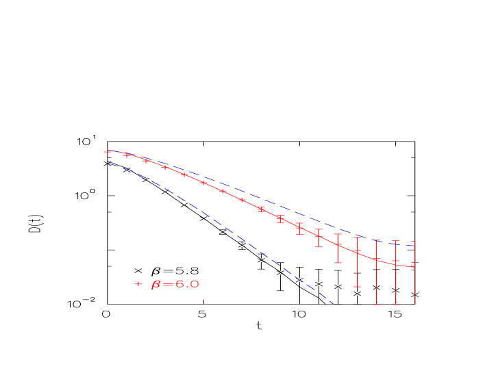
FIG. 8.: Time-slice gluon correlator, in Laplacian gauge, at $\beta=5.8$ and $6.0$. The dashed lines show Cornwall’s model fitted to $D(\hat{q}^{2})$ after the cylindrical momentum cut; the solid lines are direct fits to the time-slice correlators, excluding the first few time-slices.

We also measure the correlator of the gluon field averaged over a time-slice. Namely, we measure

$$C(t)=\frac{1}{L_{s}^{3}}\frac{1}{8}\sum_{a=1}^{8}\frac{1}{3}\sum_{\mu=1}^{3}(\sum_{x}^{L_{s}^{3}}A_{\mu}^{a}(\vec{x},0))~{}(\sum_{x}^{L_{s}^{3}}A_{\mu}^{a}(\vec{x},t))$$ (4.23)

which is displayed in Fig.8. At large time separations $t$, this correlator should decay exponentially like $exp(-m_{pole}t)$, giving us another approach to extracting the pole mass. We use this observable to perform a crosscheck on this mass, and as a further study of the systematic errors in its determination. This correlator is measured on the same configurations as $D(q^{2})$, so it contains no additional information. But the same information is given a different weight, so that a fit to $C(t)$ will give different results than a fit to $D^{-1}(q^{2})$, especially after the cylindrical momentum cut. Therefore, we fit Cornwall’s model directly to $C(t)$ instead of $D^{-1}(q^{2})$. Remarkably, the difference is rather small, which attests again to the soundness of the model. The dashed lines in Fig.8 show the original fit of Cornwall’s ansatz to $D^{-1}(q^{2})$, which already provides a fair description of the data. The solid lines represent a direct fit of the same 3-parameter ansatz to $C(t)$, excluding the first few time-slices which otherwise completely dominate the fit. The fit started from $t=4$ and $t=2$ at $\beta=6.0$ and 5.8 respectively, which amounts to discarding similar intervals in physical units. Given the 3 fitted parameters, one can then solve $D^{-1}(q^{2})=0$ numerically, with $D(q^{2})$ as per eq.(4.18). The corresponding pole mass varies little from one fit to the other, and remains roughly constant in physical units at $\beta=5.8$ and $6.0$. Also, a model-independent extraction of the pole mass, by measuring the effective mass $m_{eff}(t)=-Ln(C(t+1)/C(t))$, gives a consistent value. Taking these results into account, together with the quadratic and cubic extrapolations displayed in Fig.7, we estimate the pole mass to lie in the interval $[500,785]$ MeV, where we used $a^{-1}(\beta=6.0)=1.943$ GeV to convert to physical units [26] with $\sqrt{\sigma}=440$ MeV. The lower bound is given by the infrared mass, which corresponds to a linear extrapolation of $D^{-1}(q^{2})$; the upper bound is provided by the largest value obtained when fitting to our data Cornwall’s model. A reasonable central value is 640 MeV, which corresponds to Cornwall’s extrapolation in Fig.7.

We have performed a similar exercise for the Landau gauge. The fit of Cornwall’s model to $D(q^{2})$ or $C(t)$ is quite satisfactory, but the equation $D^{-1}(q^{2})=0$ gives a complex pole, far from the real axis. Note that Ref. [30] also finds oscillatory behaviour for the time-slice correlator in $3d$ $SU(2)$ theory fixed to Landau gauge, reflecting a complex pole. This disagreement with the Laplacian gauge is puzzling, since one expects the pole to be gauge invariant. Possible causes include the inadequacy of the Landau gauge fixing procedure on the lattice, or finite-size effects. Larger volume studies, currently under way, should elucidate this issue.

5 Conclusions

We have evaluated the gluon propagator using the Laplacian gauge which avoids lattice Gribov copies. We extracted the transverse part of the gluon propagator and verified its scaling in this gauge. Examining the scaling and volume dependence of the zero-momentum propagator ${\cal D}(0)$, we reached the conclusion that it is a constant beyond a lattice size of $\sim 0.8$ fm. This size is consistent with the characteristic length scale determined from ${\cal D}(0)$ itself as the range beyond which the gluon field decorrelates in this gauge.

Among the various proposals for the transverse propagator which are physically founded, Cornwall’s model [10] provides a reasonable fit to the lattice results over the whole momentum range. We find it satisfying that the lattice data seem to favour a model with a dynamically generated mass.

By looking at the inverse propagator $D^{-1}(q^{2})$ at small momenta, we see that the Laplacian gauge is superior to the Landau gauge in its restoration of Lorentz symmetry on the lattice. Furthermore, it turns out that the inverse propagator is almost linear in $\hat{q}^{2}$ in the Laplacian gauge. This allows for a more reliable extrapolation to $\hat{q}^{2}<0$, as compared to the Landau gauge. We test a variety of extrapolation ansätze. They consistently yield a pole mass at $\sim 640\pm 140$ MeV.

Acknowledgements: The $16^{3}\times 32$ lattice configurations were obtained from the Gauge Connection archive [27]. We thank A. Cucchieri, S. Dürr, M. Pepe and O. Philipsen for helpful discussions.

REFERENCES

- [1] J. E. Mandula, Phys. Rep. 315 (1999) 273.
- [2] S. Mandelstam, Phys. Rev. D 20 (1979) 3223.
- [3] G. B. West, Phys. Lett. B115 (1982) 468.
- [4] M. Baker, J. S. Ball and F. Zachariasen, Nucl. Phys. B186 (1981) 531,560.
- [5] N. Brown and M. R. Pennington, Phys. Rev. D38 (1988) 2266.
- [6] V. N. Gribov, Nucl. Phys. B139 (1978) 1.
- [7] M. Stingl, Phys. Rev. D34 (1986) 3863.
- [8] L. von Smekal, A. Hauck and R. Alkofer, Phys. Rev. Lett.79 (1997) 3591; Ann. Phys. 267 (1998) 1; Erratum-ibid. 269 (1998) 182.
- [9] D. Zwanziger, Phys. Lett. B257 (1991) 168.
- [10] J. M. Cornwall, Phys. Rev. D 26 (1982) 1453.
- [11] J. E. Mandula and M. Ogilvie, Phys. Lett. B 185 (1987) 127.
- [12] R. Gupta et al., Phys. Rev. D 36 (1987) 2813.
- [13] P. Marenzoni, G. Martinelli, N. Stella and M. Testa, Phys. Lett. B 318 (1993) 511; P. Marenzoni, G. Martinelli and N. Stella Nucl. Phys. B455 (1995) 339.
- [14] D. Leinweber, J. I. Skullerud, A. G. Williams, and C. Parrinello, Phys. Rev. D 60 (1999) 094507; Erratum-ibid. D 61 (2000) 079901; F.D.R. Bonnet, P.O. Bowman, D.B. Leinweber and A.G. Williams, Phys.Rev. D 62 (2000) 051501.
- [15] A. Cucchieri, Nucl. Phys. B305 (1997) 353;
- [16] T. G. Kovacs and E. T. Tomboulis, Phys. Lettt. B 463 (1999) 104.
- [17] J. C. Vink and U. Wiese, Phys. Lett. B 289 (1992) 122.
- [18] R. Kobes, G. Kunstatter and A. Rebhan, Phys. Rev. Lett. 64 (1990) 2992; Nucl. Phys. B355, 1.
- [19] L. Giusti, M. L. Paciello, S. Petrarca, B. Taglienti and M. Testa Phys. Lett. B432 (1998) 196; A. Cucchieri,Phys.Rev. D 60 (1999) 034508.
- [20] A. Cucchieri, hep-lat/9908050.
- [21] L. Del Debbio et al., Phys. Rev. D 58 (1998) 094501.
- [22] V.G. Bornyakov et al., hep-lat/0002017, JETP 71 (2000) 231; hep-lat/0009035; V.G. Bornyakov, proceedings of “Confinement 2000”, Osaka, March 2000, World Scientific pub.
- [23] J. C. Vink, Phys. Rev. D 51 (1995) 1292.
- [24] Ph. de Forcrand and M. Pepe, hep-lat/0010093.
- [25] P. van Baal, Nucl. Phys. Proc. Suppl. 42 (1995) 843.
- [26] G.S. Bali and K. Schilling, Phys. Rev. D 47, 661 (1993).
- [27] http://qcd.nersc.gov.
- [28] R. Gupta et al., Phys. Rev. D 36 (1987) 2813; Ph. de Forcrand and R. Gupta, Nucl. Phys. B (Proc. Suppl.) 9 (1989) 516.
- [29] C. Alexandrou, Ph. de Forcrand and E. Follana, hep-lat/0009003, Quark confinement and the Hadron spectrum IV, July 3-8, 2000, Vienna, Austria, Conference proceedings, World Scientific Publishing Co. (in press).
- [30] A. Cucchieri, F. Karsch and P. Petreczky, hep-lat/0004027.