Quenched Lattice QCD with Domain Wall Fermions and the Chiral Limit

Abstract

Quenched QCD simulations on three volumes, $8^{3}\times$, $12^{3}\times$ and $16^{3}\times 32$ and three couplings, $\beta=5.7$, 5.85 and 6.0 using domain wall fermions provide a consistent picture of quenched QCD. We demonstrate that the small induced effects of chiral symmetry breaking inherent in this formulation can be described by a residual mass ($m_{\rm res}$) whose size decreases as the separation between the domain walls ($L_{s}$) is increased. However, at stronger couplings much larger values of $L_{s}$ are required to achieve a given physical value of $m_{\rm res}$. For $\beta=6.0$ and $L_{s}=16$, we find $m_{\rm res}/m_{s}=0.033(3)$, while for $\beta=5.7$, and $L_{s}=48$, $m_{\rm res}/m_{s}=0.074(5)$, where $m_{s}$ is the strange quark mass. These values are significantly smaller than those obtained from a more naive determination in our earlier studies. Important effects of topological near zero modes which should afflict an accurate quenched calculation are easily visible in both the chiral condensate and the pion propagator. These effects can be controlled by working at an appropriately large volume. A non-linear behavior of $m_{\pi}^{2}$ in the limit of small quark mass suggests the presence of additional infrared subtlety in the quenched approximation. Good scaling is seen both in masses and in $f_{\pi}$ over our entire range, with inverse lattice spacing varying between 1 and 2 GeV.

I Introduction

Since spontaneous chiral symmetry breaking is a dominant property of the QCD vacuum and is responsible for much of the low energy physics seen in Nature, having a first principles formulation of lattice QCD which does not explicitly break chiral symmetry has been an important goal. Both Wilson and staggered fermions recover chiral symmetry in the continuum limit but with these techniques the chiral and continuum limits cannot be decoupled. For the QCD phase transition, which is dominantly a chiral symmetry restoring transition, a formulation that is free of violations of chiral symmetry due to lattice artifacts, should give a phase transition more closely approximating that of the continuum limit. For the measurement of matrix elements of operators in hadronic states, a formulation that respects chiral symmetry on the lattice substantially reduces operator mixing through renormalization. Lastly, since much of our analytic understanding of low-energy QCD is formulated in terms of low-energy effective field theories based on chiral symmetry, a lattice formulation preserving chiral symmetry allows controlled comparison with analytic expectations.

Building on the work of Kaplan [1], who showed how to produce light chiral modes in a $d$ dimensional theory as surface states in a $d+1$ dimensional theory, a number of attractive lattice formulations have been developed which achieve a decoupling of the continuum and chiral limits. Here we will use Kaplan’s approach as was further developed by Narayanan and Neuberger [2, 3, 4, 5] and by Shamir [6]. It is Shamir’s approach, commonly known as the domain wall fermion formulation, which we adopt. (For reviews of this topic see Refs. [7, 8, 9, 10, 11] and for more extensive recent references see Ref. [12].) For a physical four-dimensional problem, the domain wall fermion Dirac operator, $D$, is a five-dimensional operator with free boundary conditions for the fermions in the new fifth dimension. The desired light, chiral fermions appear as states exponentially bound to the four-dimensional surfaces at the ends of the fifth dimension. The remaining modes for $D$ are heavy and delocalized in the fifth dimension.

An additional important feature of the domain wall fermion Dirac operator in the limit $L_{s}\rightarrow\infty$ is the existence of an “index”, an integer that is invariant under small changes in the background gauge field. Here $L_{s}$ is the extent of the lattice in the fifth dimension. This property, true for all but a set of gauge fields of measure zero, can be readily seen using the overlap formalism [2, 3, 4, 5]. In the smooth background field limit, this index is the normal topological charge but, even for rough fields, it signals the presence of massless fermion mode(s) when non-zero. These zero modes can easily be recognized in numerical studies with semiclassical gauge field backgrounds [13, 14, 15, 16, 17, 18].

These powerful theoretical developments in fermion formulations require additional study to demonstrate their merit for numerical work. For the case of domain wall fermions, a growing body of numerical results are available. Both quenched [17, 19, 20, 21, 22, 23, 24, 25, 26, 27, 28, 29, 30, 31] and dynamical [31, 32, 33, 34, 35, 12] domain wall fermion simulations have been conducted and the domain wall approach is readily adapted to current algorithms for lattice QCD. (Much work is also being done on the numerical implementation of the overlap formulation and its variations [36, 37, 38, 39, 40, 41, 42, 43, 44, 45, 46].) A fundamental question, which is a major part of this paper, involves quantifying the residual chiral symmetry breaking effects of finite extent in the fifth dimension.

Due to current limits on computer speed, some lattice QCD studies are only practical when the fermionic determinant is left out of the measure of the path integral. The resulting quenched theory does not suppress gauge field configurations with light fermionic modes, in contrast with the original theory where, for small quark mass, the determinant strongly damps such configurations. The measurement of observables involving fermion propagation through configurations with unsuppressed light fermionic modes can in principle lead to markedly different infrared behavior than that found in full QCD, in the limit of small quark masses. Domain wall fermions, which produce light chiral modes at finite lattice spacing and preserve the global symmetries of continuum QCD, should produce a well-defined chiral limit for full QCD. The central question addressed in this paper is whether a well-controlled chiral limit also exists within the quenched approximation. A thorough theoretical and numerical understanding of the quenched chiral limit is essential if the good chiral properties of domain wall fermions are to be exploited in quenched lattice simulations.

Here we present results from extensive simulations of quenched QCD with domain wall fermions, primarily at two lattice spacings, $a^{-1}\sim 1$ and 2 GeV. Many different values for the fifth dimensional extent, $L_{s}$, and the bare quark mass, $m_{f}$ have been used. Hadron masses, $f_{\pi}$ and the chiral condensate, $\langle\overline{q}q\rangle$, are the primary hadronic observables we have studied. In calculating physical observables using domain wall fermions, four-dimensional quark fields $q(x)$ are defined from the five-dimensional fields $\Psi(x,s)$ by taking the left-handed fields from the four-dimensional hypersurface with smallest coordinate in the fifth dimension and the right-handed fields from the hypersurface with the largest value of this coordinate. We also present results from measuring the lowest eigenvectors and eigenvalues of the hermitian domain wall fermion operator.

Here we list the major topics in each section of this paper. Section II defines our conventions and gives details of the hermitian domain wall fermion operator. Section III discusses our simulation parameters and fitting procedures and includes tables of run parameters and hadron masses for $m_{f}\geq 0.01$. In Section IV a precise understanding of how finite $L_{s}$ effects enter $\langle\overline{q}q\rangle$ is developed and measurements of $\langle\overline{q}q\rangle$ which show the role of fermionic zero modes are reported. We study the pion mass in the chiral limit in Section V, which requires understanding zero mode effects. Section VI contains two determinations of the residual chiral symmetry breaking for finite $L_{s}$; one from measuring appropriate pion correlators and the other from the explicitly measured small eigenvalues and eigenvectors of the hermitian domain wall fermion operator. Our determination of $f_{\pi}$, an important check of the chiral properties of domain wall fermions, is discussed in Section VII, along with the scaling of hadron masses.

Because of the length of this paper and the number of topics covered, we now give a brief summary of our major results, organized to correspond to the expanded discussion in Sections IV, V VI and VII.

Zero mode effects in $\langle\overline{q}q\rangle$: As already mentioned, the domain wall fermion operator $D$ has an Atiyah-Singer index $\nu$ for $L_{s}\rightarrow\infty$. However, in quenched QCD, $\nu$ plays no role in the generation of gauge field configurations. For $\nu\neq 0$, both $D$ and the hermitian domain wall fermion operator $D_{H}$ [47] have zero modes. Since $\langle\overline{q}q\rangle$ is an appropriately restricted trace of $D_{H}^{-1}$ it should diverge as $\langle|\nu|\rangle/m_{f}V$ for small $m_{f}$ if the ensemble average of $|\nu|$ is non-zero. Here $V$ is the four-dimensional, space-time volume of the lattice being studied. For large but finite $L_{s}$, the residual chiral symmetry breaking should cut off this divergence.

Figure 1 shows $\langle\overline{q}q\rangle$ versus the quark mass $m_{f}$ for $a^{-1}\sim 1$ GeV on two different volumes of linear dimensions of about 1.6 and 3.2 Fermi. A divergence for $m_{f}\rightarrow 0$ is clearly visible on the smaller volume, but not on the larger. This is expected since $\langle|\nu|\rangle/V$ should go as $1/\sqrt{V}$ and is clear evidence for unsuppressed zero modes in quenched QCD, first reported in Ref. [22]. Notice that there may be other problems with the chiral limit of $\langle\overline{q}q\rangle$ that are masked by this $1/m_{f}$ divergence.

The chiral limit of $m_{\pi}$: With this clear evidence for zero mode effects in $\langle\overline{q}q\rangle$, one might expect to see zero mode contributions in any quark propagator $D^{-1}(x,y)$ if at both $x$ and $y$ a single zero eigenvector has reasonable magnitude. For sufficiently large volume, needed to see asymptotic behavior in the limit of large $|x-y|$, there should be no zero mode effects. Our results for the zero mode effects on the pion mass are presented in Figure 2 which shows $m_{\pi}^{2}$ versus $m_{f}$ for $8^{3}\times 32$ lattices with $L_{s}=48$ and Figure 3, where all the parameters are the same except that the volume was increased to $16^{3}\times 32$. The pion mass is determined from three different correlators which are each affected differently by zero modes. For the smaller volume, the pion masses measured disagree for small $m_{f}$, while they agree for the larger volume.

Notice that on the larger volume shown in Figure 3, where zero-mode effects are not apparent, $m_{\pi}^{2}$ shows signs of curvature in $m_{f}$ with the three $m_{f}=0$ values lying below the extrapolation from larger masses. In addition, this simple large-mass linear extrapolation vanishes at a value of $m_{f}$ that is more negative than the point $m_{f}+m_{\rm res}=0$ (shown in the graph by the star) also suggesting downward concavity. While the discrepancy between this $x$-intercept and the point $m_{f}+m_{\rm res}=0$, may be caused by $O(a^{2})$ effects, we find a considerably larger discrepancy when making a similar comparison at $\beta=6.0$. Thus, we have evidence that $m_{\pi}^{2}$ does not depend linearly on $m_{f}$ in the chiral limit.

Determining the residual mass: In the limit of small lattice spacing, the dominant chiral symmetry breaking effect, due to the mixing between the domain walls, is the appearance of a residual mass, $m_{\rm res}$ in the low energy effective Lagrangian. The Ward-Takahashi identity for domain wall fermions [47] has an additional contribution representing this explicit chiral symmetry breaking due to finite $L_{s}$. Matrix elements of this additional term between low energy states determine the residual quark mass. Figure 4 shows our results for $m_{\rm res}$ for $16^{3}\times 32$ lattices at $\beta=6.0$ as a function of $L_{s}$. $m_{\rm res}$ is clearly falling with $L_{s}$ and reaches a value of $\sim 2$ MeV for $L_{s}\geq 24$. Our data does not resolve the precise behavior of $m_{\rm res}$ for large $L_{s}$, but the very small value makes this less important for current simulations. A similar study on lattices with $a^{-1}\sim 1$ GeV but with larger $L_{s}=48$ finds a value of $m_{\rm res}/m_{s}=0.074(5)$ or $m_{\rm res}\approx 8$ MeV.

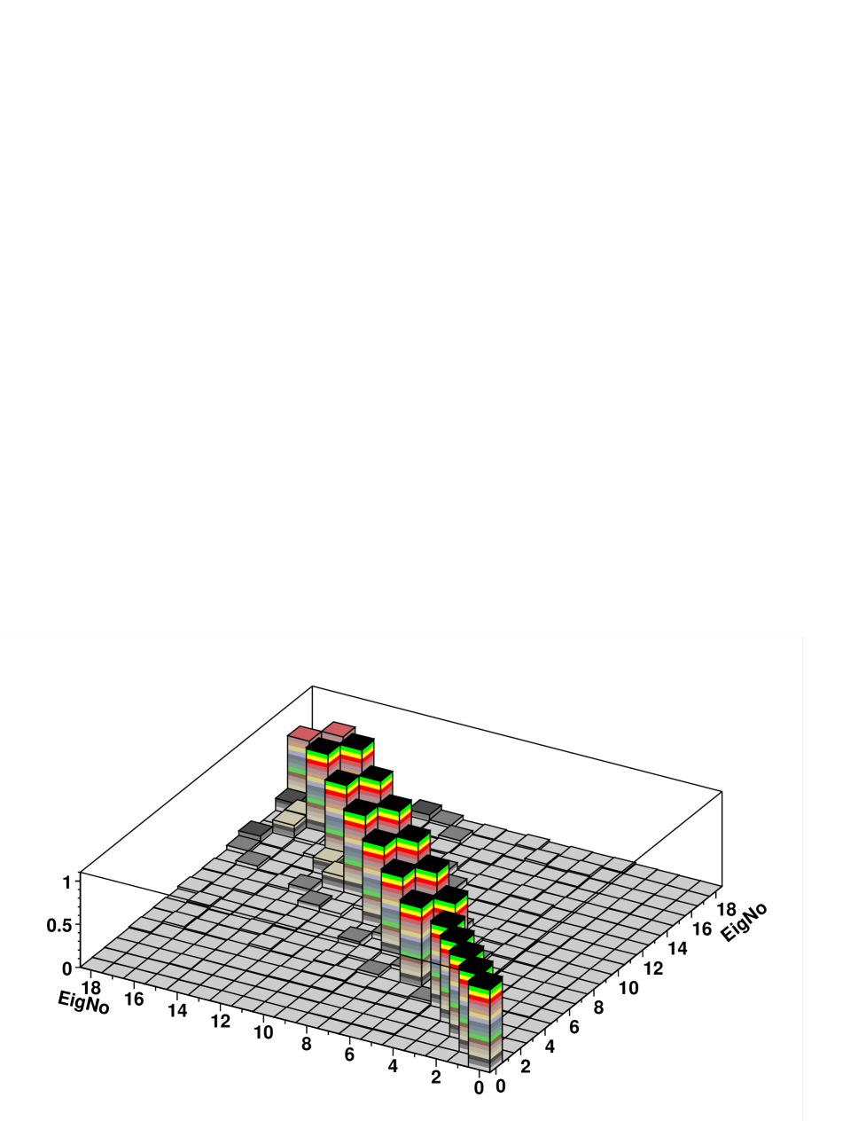
We have also used the Rayleigh-Ritz method, implemented using the technique of Kalk-Reuter and Simma [48], to determine the low-lying eigenvalues and eigenvectors for the hermitian domain wall fermion operator. The results exhibit the approximate behavior expected from low-energy excitations in the domain wall formulation. We use the resulting eigenvalues to provide an independent estimate of the residual mass which is nicely consistent with the more precise value determined from pseudoscalar correlators.

Results for $f_{\pi}$, hadron masses and scaling: With this detailed understanding of the chiral limit of quenched lattice QCD with domain wall fermions, we have calculated $f_{\pi}$ using both pseudoscalar and axial-vector correlators. The results for lattices with $a^{-1}\sim 2$ GeV are shown in Figure 5, where good agreement between the two methods is seen. To do this comparison, the appropriate Z-factor for the local axial current must be determined and a consistent value for $m_{\rm res}$ must be known. The good agreement in the figure is a significant test of these measurements as well as the chiral properties of domain wall fermions. We find very good scaling in the ratio $f_{\pi}/m_{\rho}$ for $a^{-1}\sim 1$ to 2 GeV. For $m_{N}/m_{\rho}$ scaling is within 6%. We also find that $-\langle\overline{q}q\rangle=(256(8){\rm MeV})^{3}$ from our $\beta=6.0$ simulations.

II Domain wall fermions

In this section we first define our notation, including the domain wall fermion Dirac operator, and then derive the precise form of the Banks-Casher relation for domain wall fermions, to second order in the quark mass. In this paper, the variable $x$ specifies the coordinates in the four-dimensional space-time volume, with extent $L$ along each of the spatial directions and extent $N_{t}$ along the time direction, while $s=0,1,\dots,L_{s}-1$ is the coordinate of the fifth direction, with $L_{s}$ assumed to be even. The space-time volume $V$ is given by $V=L^{3}N_{t}$. The domain wall fermion operator acts on a five-dimensional fermion field, $\Psi(x,s)$, which has four spinor components. A generic four-dimensional fermion field, with four spin components, will be denoted by $\psi(x)$, while the specific four-dimensional fermion field defined from $\Psi(x,s)$ will be denoted by $q(x)$. The space-time indices for vectors will be enclosed in parenthesis while for matrices they will be given as subscripts. Our general formalism follows that developed by Furman and Shamir [47].

A Conventions

The domain wall fermion operator is given by

$$D_{x,s;x^{\prime},s^{\prime}}=\delta_{s,s^{\prime}}D^{\parallel}_{x,x^{\prime}}+\delta_{x,x^{\prime}}D^{\bot}_{s,s^{\prime}}$$ (1)

$$D^{\parallel}_{x,x^{\prime}} = {1\over 2}\sum_{\mu=1}^{4}\left[(1-\gamma_{\mu})U_{x,\mu}\delta_{x+\hat{\mu},x^{\prime}}+(1+\gamma_{\mu})U^{\dagger}_{x^{\prime},\mu}\delta_{x-\hat{\mu},x^{\prime}}\right]$$ (2)

$$+ (M_{5}-4)\delta_{x,x^{\prime}}$$ (3)

$$D^{\bot}_{s,s^{\prime}} = {1\over 2}\Big{[}(1-\gamma_{5})\delta_{s+1,s^{\prime}}+(1+\gamma_{5})\delta_{s-1,s^{\prime}}-2\delta_{s,s^{\prime}}\Big{]}$$ (4)

$$- {m_{f}\over 2}\Big{[}(1-\gamma_{5})\delta_{s,L_{s}-1}\delta_{0,s^{\prime}}+(1+\gamma_{5})\delta_{s,0}\delta_{L_{s}-1,s^{\prime}}\Big{]}.$$ (5)

Here, $U_{x,\mu}$ is the gauge field at site $x$ in direction $\mu$, and $s$ and $s^{\prime}$ lie in the range $0\leq s,s^{\prime}\leq L_{s}-1$. The five-dimensional mass, representing the height of the domain wall in Kaplan’s original language, is given by $M_{5}$, while $m_{f}$ directly couples the two domain walls at $s=0$ and $s=L_{s}-1$. Since the light chiral modes should be exponentially bound to the domain walls, $m_{f}$ mixes the two chiralities and is therefore the input bare quark mass. The value of $M_{5}$ must be chosen to produce these light surface states and, in the free field case, $0<M_{5}<2$ produces a single fermion flavor with the left-hand chirality bound to $s=0$ and the right to $s=L_{s}-1$. In order to use our pre-existing, high-performance Wilson fermion operator computer program as part of our domain wall fermion operator, we have used the operator $D$ above, which is the same as $D_{F}^{\dagger}$ of Ref. [47].

Following Ref. [47], we define the four-dimensional quark fields $q(x)$ by

$$q(x) = P_{\rm L}\Psi(x,0)+P_{\rm R}\Psi(x,L_{s}-1)$$ (6)

$$\bar{q}(x) = \overline{\Psi}(x,L_{s}-1)P_{\rm L}+\overline{\Psi}(x,0)P_{\rm R}$$ (7)

where we have used the projection operators $P_{R,L}=(1\pm\gamma_{5})/2$. Symmetry transformations of the five-dimensional fields yield a four-dimensional axial current

$${\cal A}^{a}_{\mu}(x)=\sum_{s=0}^{L_{s}-1}{\rm sign}\left(s-\frac{L_{s}-1}{2}\right)j^{a}_{\mu}(x,s).$$ (8)

Here

$$j^{a}_{\mu}(x,s)=\frac{1}{2}\left[\overline{\Psi}(x+\hat{\mu},s)(1+\gamma_{\mu})U^{\dagger}_{x+\hat{\mu},\mu}t^{a}\Psi(x,s)-\overline{\Psi}(x,s)(1-\gamma_{\mu})U_{x,\mu}t^{a}\Psi(x+\hat{\mu},s)\right]$$ (9)

while the flavor matrices are normalized to obey ${\rm Tr}\,(t^{a}t^{b})=\delta^{ab}$. The divergence of this current satisfies

$$\Delta_{\mu}{\cal A}^{a}_{\mu}(x)=2m_{f}J^{a}_{5}(x)+2J^{a}_{5q}(x)$$ (10)

where $\Delta_{\mu}f(x)=f(x)-f(x-\hat{\mu})$ is a simple finite difference operator and the pseudoscalar density $J^{a}_{5}(x)$ is

$$J^{a}_{5}(x) = -\overline{\Psi}(x,L_{s}-1)P_{\rm L}t^{a}\Psi(x,0)+\overline{\Psi}(x,0)P_{\rm R}t^{a}\Psi(x,L_{s}-1)$$ (11)

$$= \overline{q}(x)t^{a}\gamma_{5}q(x).$$ (12)

This equation differs from the corresponding continuum expression by the presence of the $J^{a}_{5q}(x)$ term, which is built from point-split operators at $L_{s}/2$ and $L_{s}/2-1$ and is given by

$$J^{a}_{5q}(x)=-\overline{\Psi}(x,L_{s}/2-1)P_{\rm L}t^{a}\Psi(x,L_{s}/2)+\overline{\Psi}(x,L_{s}/2)P_{\rm R}t^{a}\Psi(x,L_{s}/2-1).$$ (13)

We will refer to this term as the “mid-point” contribution to the divergence of the axial current.

This mid-point term adds an additional term to the axial Ward-Takahashi identities and modifies observables, like the pion mass, which are controlled by these identities. The Ward-Takahashi identity is

$$\Delta_{\mu}\langle{\cal A}^{a}_{\mu}(x)O(y)\rangle=2m_{f}\langle J^{a}_{5}(x)O(y)\rangle+2\langle J^{a}_{5q}(x)O(y)\rangle+i\langle\delta^{a}O(y)\rangle.$$ (14)

For operators, $O$ made from the fields $q(y)$ and $\overline{q}(y)$, it has been shown [47] that the $J^{a}_{5q}$ term in Eq. 14 vanishes for flavor non-singlet currents when $L_{s}\rightarrow\infty$. For the singlet current, this extra term generates the axial anomaly. The mid-point term represents the contribution of finite $L_{s}$ effects on the low-energy physics of domain wall fermions.

B Definition of the residual mass and the chiral limit

For domain wall fermions, the axial transformation which leads to the Ward-Takahashi identity of Eq. 14 rotates the fermions in the two half-spaces along the fifth direction with opposite charges. For $m_{f}=0$, the action is not invariant under this transformation due to the coupling of the left- and right-handed light surface states at the midpoint of the fifth dimension. This results in the additional term in the divergence of the axial current, as given in Eq. 13. In the $L_{s}\rightarrow\infty$ limit where the explicit mixing between the $s\sim 0$ and $s\sim L_{s}-1$ states vanishes, this extra “mid-point” contribution will be zero and a continuum-like Ward-Takahashi identity will be realized.

Since we must work at finite $L_{s}$ it is useful to characterize the chiral symmetry breaking effects of mixing between the domain walls as precisely as possible. We do this by adopting the language of the Symanzik improvement program [49, 50]. Here we use an effective continuum Lagrangian ${\cal L}_{n}$ to reproduce to $O(a^{n})$ the amplitudes predicted by our lattice theory when evaluated at low momenta and finite lattice spacing. Clearly ${\cal L}_{0}$ is simply the continuum QCD Lagrangian, while ${\cal L}_{1}$ will include the dimension-five, clover term: $\overline{\psi}\sigma^{\mu\nu}\psi F_{\mu\nu}$ [51]. The chiral symmetry breaking effects of mixing between the domain walls will appear to lowest order in $a$ as an additional, dimension three operator $\propto a^{-1}e^{-\alpha L_{s}}\;\overline{\psi}\psi$. This term represents the residual mass term that remains even after the explicit input chiral symmetry breaking parameter $m_{f}$ has been set to zero. The next chiral symmetry breaking contribution from domain wall mixing will be $O(a^{2})$ smaller, appearing as a coefficient of order $a^{1}$ for the clover term.

We define the chiral symmetry breaking parameter $m_{\rm res}$ so the complete coefficient of the mass term in ${\cal L}_{0}$ is proportional to the simple sum $m_{f}+m_{\rm res}$. While this is a precise definition of $m_{\rm res}$, valid for finite lattice spacing, a precise determination of $m_{\rm res}$ in a lattice calculation will be impeded by the need to quantitatively account for the additional chiral symmetry breaking effects of terms of higher order in $a$.

Close to the continuum limit, for long distance amplitudes, the Ward-Takahashi identity given in Eq. 14 must agree with the corresponding identity in the effective continuum theory. Thus, for the non-singlet case, the sum of the first two terms on the right-hand side of Eq. 14 must be equivalent to an effective quark mass, $m_{\rm eff}=m_{f}+m_{\rm res}$, times the pseudo-scalar density $J_{5}^{a}$. Thus, the residual mass, $m_{\rm res}$ appears in the low energy identity:

$$J^{a}_{5q}\approx m_{\rm res}J^{a}_{5}$$ (15)

where this equality will hold up to $O(a^{2})$ in low-momentum amplitudes.

Thus, close to the continuum limit, $m_{\rm res}$ in Eq. 15 is a universal measure of the chiral symmetry breaking effects of domain wall fermions for all low energy matrix elements, with corrections coming from terms of higher order in the lattice spacing. However, away from the continuum limit the $O(a^{2})$ terms may be appreciable. In addition, if there are high energy scales entering an observable, such a low energy description is not valid and the explicit chiral symmetry breaking effects of finite $L_{s}$ can be more complicated than a simple additive shift of the input quark mass by $m_{\rm res}$.

Many aspects of the chiral behavior of the domain wall theory can be easily understood by reference to the more familiar Wilson fermion formulation. For finite $L_{s}$ the domain wall formulation can be viewed as an “on- and off-shell improved” version of Wilson fermions. The low energy effective Lagrangian for domain wall fermions is the same as that for the Wilson case except the coefficients of the chiral symmetry breaking terms are expected to decrease exponentially with $L_{s}$. Viewed in this way, one might expect to achieve a vanishing pion mass by fine-tuning $m_{f}$ to a critical value, $m_{fc}$ in very much the same way as one fine-tunes $\kappa$ to $\kappa_{c}$ for Wilson fermions. As the above discussions demonstrates, $m_{fc}=m_{\rm res}+O(a^{2})$. Just as in the Wilson case, this limit can be interpreted as the approach to the critical surface of the Aoki phase [34, 29, 30].

C The hermitian domain wall fermion operator

A hermitian operator $D_{H}$ can be constructed [47] from $D$ through

$$D_{H}\equiv\gamma_{5}R_{5}D$$ (16)

where $(R_{5})_{ss^{\prime}}\equiv\delta_{s,L_{s}-1-s^{\prime}}$ is the reflection in the fifth dimension around the five-dimensional midpoint, $s=(L_{s}-1)/2$. Writing out $D_{H}$ gives

$$D_{H} = \gamma_{5}\,D^{\parallel}_{x,x^{\prime}}\,\delta_{s+s^{\prime},L_{s}-1}$$ (17)

$$+ \gamma_{5}\left[P_{L}\,\delta_{s+s^{\prime},L_{s}}+P_{R}\,\delta_{s+s^{\prime},L_{s}-2}-\delta_{s+s^{\prime},L_{s}-1}\right.$$ (18)

$$- \left.m_{f}(P_{L}\,\delta_{s,0}\delta_{s^{\prime},0}+P_{R}\,\delta_{s,L_{s}-1}\delta_{s^{\prime},L_{s}-1})\right]\delta_{x,x^{\prime}}$$ (19)

while as an explicit matrix in the $s,s^{\prime}$ indices:

$$D_{H}=\left(\begin{array}[]{cccccc}-m_{f}\gamma_{5}P_{L}&&&&\gamma_{5}P_{R}&\gamma_{5}(D^{\parallel}-1)\\ &&&\gamma_{5}P_{R}&\gamma_{5}(D^{\parallel}-1)&\gamma_{5}P_{L}\\ &&\cdots&\cdots&\cdots&\\ &\cdots&\cdots&\cdots&&\\ \gamma_{5}P_{R}&\gamma_{5}(D^{\parallel}-1)&\gamma_{5}P_{L}&&&\\ \gamma_{5}(D^{\parallel}-1)&\gamma_{5}P_{L}&&&&-m_{f}\gamma_{5}P_{R}\\ \end{array}\right).$$ (20)

The eigenfunctions and eigenvectors of $D_{H}$ will be denoted by

$$D_{H}\Psi_{\Lambda_{H}}=\Lambda_{H}\Psi_{\Lambda_{H}}$$ (21)

with the five-dimensional propagator given by

$$S^{(5)}_{x,s;x^{\prime},s^{\prime}}=\sum_{\Lambda_{H}}\frac{\Psi_{\Lambda_{H}}(x,s)\Psi^{\dagger}_{\Lambda_{H}}(x^{\prime},\tilde{s})\,\gamma_{5}\,(R_{5})_{\tilde{s},s^{\prime}}}{\Lambda_{H}}.$$ (22)

(Grassmann variables in the Euclidean path integral will be denoted by $\overline{\Psi}$ and $\Psi$, while the eigenfunctions of $D_{H}$ will be denoted $\Psi^{\dagger}_{\Lambda_{H}}$ and $\Psi_{\Lambda_{H}}$.)

We will find it convenient to define three additional matrices

$$(\Gamma_{5})_{s,s^{\prime}}=\delta_{s,s^{\prime}}\,{\rm sign}\left(\frac{L_{s}-1}{2}-s\right)$$ (23)

$$Q^{\rm(w)}_{s,s^{\prime}}=P_{L}\,\delta_{s,0}\,\delta_{s^{\prime},0}+P_{R}\,\delta_{s,L_{s}-1}\,\delta_{s^{\prime},L_{s}-1}$$ (24)

and

$$Q^{\rm(mp)}_{s,s^{\prime}}=P_{L}\,\delta_{s,L_{s}/2}\,\delta_{s^{\prime},L_{s}/2}+P_{R}\,\delta_{s,L_{s}/2-1}\,\delta_{s^{\prime},L_{s}/2-1}.$$ (25)

The transformation which generates the current in Eq. 8 is

$$\Psi \rightarrow \exp(i\alpha^{a}t^{a}\Gamma_{5})\Psi$$ (26)

$$\overline{\Psi} \rightarrow \overline{\Psi}\exp(-i\alpha^{a}t^{a}\Gamma_{5}).$$ (27)

The matrices $Q^{\rm(w)}$ and $Q^{\rm(mp)}$ are the two parts of $D_{H}$ which correspond to terms in $D=\gamma_{5}R_{5}D_{H}$ which are not invariant under the transformation in Eq. 27. The matrix $Q^{\rm(w)}$ underlies the explicit mass term and, in the original operator $D$, explicitly mixes the $s=0$ and $s=L_{s}-1$ walls. Likewise, the matrix $Q^{\rm(mp)}$ is a “mid-point” matrix with non-zero elements only in the center of the fifth dimension. It represents the component of the operator $D$ which connects the left and right half regions. These two contributions provide the terms on the right hand side of Eq. 10 and one easily finds

$$\{\Gamma_{5},D_{H}\}=2m_{f}Q^{\rm(w)}+2Q^{\rm(mp)}.$$ (28)

Since it is expected that there are eigenvectors of $D_{H}$ which are exponentially localized on the domain walls, we see that with $m_{f}=0$ and the limit $L_{s}\rightarrow\infty$ taken, $D_{H}$ anticommutes with $\Gamma_{5}$ in the subspace of these eigenvectors. This is the property expected for massless, four-dimensional fermions in the continuum in Euclidean space.

Using the matrix, $Q^{\rm(w)}$, we can write a simple form for the four-dimensional chiral condensate, $\langle\overline{q}q\rangle$

$$-\langle\overline{q}q\rangle = -\frac{1}{12V}\sum_{x}\langle\overline{q}(x)q(x)\rangle$$ (29)

$$= -\frac{1}{12V}\sum_{x}\langle\,\overline{\Psi}(x,s)(R_{5}Q^{\rm(w)})_{s,s^{\prime}}\Psi(x,s^{\prime})\rangle$$ (30)

$$= \frac{1}{12V}\left\langle\sum_{x,\Lambda_{H}}\frac{\Psi^{\dagger}_{\Lambda_{H}}(x,s)\,\gamma_{5}\,Q^{\rm(w)}_{s,s^{\prime}}\Psi_{\Lambda_{H}}(x,s^{\prime})}{\Lambda_{H}}\right\rangle$$ (31)

$$= \frac{1}{12V}\left\langle\sum_{\Lambda_{H}}\frac{\langle\Lambda_{H}|\gamma_{5}Q^{\rm(w)}|\Lambda_{H}\rangle}{\Lambda_{H}}\right\rangle$$ (32)

where in the last line a bra/ket notation has been used. The large angle brackets indicate the average over an appropriate ensemble of gauge fields.

We define the pion interpolating field as $\pi^{a}(x)\equiv i\overline{q}(x)t^{a}\gamma_{5}q(x)$ and then find that the pion two-point function is given by (no sum on $a$)

$$\langle\pi^{a}(x)\pi^{a}(0)\rangle=\left\langle\sum_{\Lambda_{H},\Lambda_{H}^{\prime}}\frac{\Psi^{\dagger}_{\Lambda_{H}^{\prime}}(x,s)\,Q^{\rm(w)}_{s,s^{\prime}}\,\Psi_{\Lambda_{H}}(x,s^{\prime})\;\Psi^{\dagger}_{\Lambda_{H}}(0,\tilde{s})\,Q^{\rm(w)}_{\tilde{s},\tilde{s}^{\prime}}\,\Psi_{\Lambda_{H}^{\prime}}(0,\tilde{s}^{\prime})}{\Lambda_{H}\Lambda_{H}^{\prime}}\right\rangle.$$ (33)

Note that the generators, $t^{a}$, do not appear in the spectral sum, since they merely serve to specify the contractions of the quark propagators and that $\pi^{a}(x)=iJ^{a}_{5}(x)$. To investigate the extra term in the axial Ward-Takahashi identity, Eq. 14, we will also have need to measure the correlation function between interpolating pion fields defined on the domain walls and the mid-point contribution to the divergence of the axial current, $J^{a}_{5q}$. We define a mid-point pion interpolating field by $\pi_{\rm(mp)}^{a}(x)=iJ^{a}_{5q}(x)$ and the spectral decomposition for the correlator between interpolating pion operators on the wall and the midpoint is

$$\langle\pi_{\rm(mp)}^{a}(x)\pi^{a}(0)\rangle=\left\langle\sum_{\Lambda_{H},\Lambda_{H}^{\prime}}\frac{\Psi^{\dagger}_{\Lambda_{H}^{\prime}}(x,s)\,Q^{\rm(mp)}_{s,s^{\prime}}\,\Psi_{\Lambda_{H}}(x,s^{\prime})\;\Psi^{\dagger}_{\Lambda_{H}}(0,\tilde{s})\,Q^{\rm(w)}_{\tilde{s},\tilde{s}^{\prime}}\,\Psi_{\Lambda_{H}^{\prime}}(0,\tilde{s}^{\prime})}{\Lambda_{H}\Lambda_{H}^{\prime}}\right\rangle.$$ (34)

We define a local axial current as $A^{a}_{\mu}(x)\equiv\overline{q}(x)t^{a}\gamma_{\mu}\gamma_{5}q(x)$ and note that it is different from ${\cal A}^{a}_{\mu}$ defined in Eq. 8. The two-point function of the zeroth component of this current, $\langle A_{0}^{a}(x)A_{0}^{a}(0)\rangle$, has a form similar to Eq. 33 with a factor of $\gamma_{0}$ multiplying each $Q^{\rm(w)}$ and an overall minus sign. Finally, our scalar density is $\sigma(x)\equiv\overline{q}(x)q(x)$ and the connected correlator $\langle\sigma(x)\sigma(0)\rangle_{\rm c}$ also has the form of Eq. 33 with a factor of $\gamma_{5}$ multiplying each $Q^{\rm(w)}$ and an overall minus sign.

III Hadron Masses for $m_{f}\geq 0.01$

In this section we present the results for $m_{\pi}$, $m_{\rho}$ and $m_{N}$ obtained for reasonably heavy input quark mass, $m_{f}\geq 0.01$ where the lower limit corresponds to $m_{\rm quark}\approx m_{\rm strange}/4$. The more challenging study of $m_{\pi}$ for $m_{f}\rightarrow 0$ is described later, in Section V. This section is organized as follows. We begin by describing the Monte Carlo runs on which the results in this paper are based. Next the methods used to determine the hadron masses are discussed, both the propagator determinations and our fitting procedures. Finally, we present the results of those calculations for the easier, large mass case, $m_{f}\geq 0.01$.

A Simulation summary

The results reported in this paper were obtained from ensembles of gauge field configuration generated from pure gauge simulations using the standard Wilson action[52] at three values of the coupling parameter, $\beta=6/g^{2}$: 5.7, 5.85 and 6.00. Thus, these ensembles follow the distribution, $\exp{\{{6/g^{2}}\sum_{\cal P}{\rm tr}U_{\cal P}\}}$ where the sum ranges over all elementary plaquettes ${\cal P}$ in the lattice and $U_{\cal P}$ is the ordered product of the four link matrices associated with the edges of the plaquette ${\cal P}$. Some of the $\beta=5.7$ simulations and a portion of those at $\beta=5.85$ were performed using the hybrid Monte Carlo ‘$\Phi$’ algorithm [53]. These runs were performed on an $8^{3}\times 32$ space-time volume with a domain wall height $M_{5}=1.65$. Each hybrid Monte Carlo trajectory consisted of 50 steps with a step size $\Delta t=0.02$. These runs are summarized in Table I. In each case the first 2,000 hybrid Monte Carlo trajectories were discarded for thermalization before any measurements were made. After these thermalization trajectories, successive measurements of hadron masses and the chiral condensate, $\langle\overline{q}q\rangle$ were made after each group of 200 trajectories.

A second set of simulations were performed using the heatbath method of Creutz [54], adapted for $SU(3)$ using the two-subgroup technique of Cabibbo and Marinari [55] and improved for a multi-processor machine by the algorithm of Kennedy and Pendleton [56]. The first 5,000 sweeps were discarded for thermalization. These runs are described in Table II where the values of $M_{5}$ used are also given. Finally, the single $\beta=5.85$ run with $M_{5}=1.9$ was performed using the MILC code [57]. Here four over-relaxed heatbath sweeps [58, 59] with $\omega=2$ were followed by one Kennedy-Pendleton sweep, with 50,000 initial sweeps discarded for thermalization.

A portion of the $\beta=5.7$ masses described here appeared earlier in Ref. [21] while the first of the $\beta=6.0$ results appear in Refs. [60] and [26].

B Mass measurement techniques

We follow the standard procedures for determining the hadron masses from a lattice calculation, extracting these masses from the exponential time decay of Euclidean-space, two-point correlation functions. In our calculation the source may take two forms. The first is a point source

$$O_{\Gamma}^{a}(x)=\bar{q}(x)t^{a}\Gamma q(x)$$ (35)

which is usually introduced at the origin. The flavor index $a$ is introduced to make clear that we do not study the masses of flavor singlet states. For the nucleon state we use a combination of three quark fields:

$$O_{\rm P}(x)=\epsilon_{abc}u_{a}(x)[u_{b}(x)C\gamma^{5}d_{c}(x)]$$ (36)

where for simplicity we have written the source for a proton in terms of up and down quark fields, $q=u$ and $d$. Here $C$ is the $4\times 4$ Dirac charge-conjugation matrix, $\epsilon$ the anti-symmetric tensor in three dimensions and the color sum over the indices $a$, $b$ and $c$ is shown explicitly. Only these point sources are used in the $\beta=5.7$ running.

The second variety of source used in this work is a wall source. Such a source is obtained by a simple generalization of Eqs. 35 and 36 in which we replace the quark fields evaluated at the same space-time point $x=(\vec{r},t)$ with distributed fields, each of which is summed over the entire spatial volume at a fixed time $t$. Gauge covariance is maintained by introducing a gauge field dependent color matrix $V[U](\vec{r},t_{i})$ which transforms the spatial links in the time slice $t=t_{i}$ into Coulomb gauge. Thus, to construct our wall sources we simply replace the quark field $q(\vec{r},t_{i})_{c}$ by the non-local field

$$q^{w}(t_{i})_{c}=\sum_{\vec{r}}V(\vec{r},t_{i})_{c,c^{\prime}}\,q(\vec{r},t_{i})_{c^{\prime}}$$ (37)

where $c$ and $c^{\prime}$ are color indices. We use these wall sources for the $\beta=5.85$ calculations and a combination of both wall and point sources in the $\beta=6.0$ studies. The use of wall sources for these weaker coupling runs is appropriate since the physical hadron states are larger in lattice units and better overlap is achieved with the states of interest by using these extended sources.

In all cases we use a zero-momentum-projected point sink for the second operator in the correlation function. This is obtained by simply summing the operators in Eqs. 35 and 36 over all spatial positions $\vec{r}$ in a fixed time plane $t=t_{f}$. Thus, for example, we will extract the mass $m_{\Gamma}$ of the lightest meson with quantum numbers of the Dirac matrix $\Gamma$ from the large $t_{f}-t_{i}$ expression:

$$\Big{\langle}\sum_{\vec{r}}O_{\Gamma}^{a}(\vec{r},t_{f})\bar{q}^{w}(t_{i})\Gamma t^{a}q^{w}(t_{i})\Big{\rangle}\sim A(e^{-m_{\Gamma}(t_{f}-t_{i})}+e^{-m_{\Gamma}(N_{t}-t_{f}+t_{i})}).$$ (38)

A similar equation is used for the nucleon correlation function except that the second exponent representing the state propagating through the antiperiodic boundary condition connecting $t=0$ and $t=N_{t}-1$ is reversed in sign and has exchanged upper and lower components for a spinor basis in which $\gamma^{0}$ is diagonal.

For both the calculation of the quark propagators from which these hadron correlators are constructed and the evaluation of the chiral condensate, $\langle\overline{q}q\rangle$, we invert the five-dimensional domain wall fermion Dirac operator of Eq. 1, using the conjugate gradient method to solve an equation of the form $Dy=h$. This iterative method is run until a stopping condition is satisfied, which requires that the norm squared of the residual be a fixed, small fraction $\epsilon$ of the norm squared of the source vector $h$. At the $n^{th}$ iteration, we determine the residual $r_{n}$ as a cumulative approximation to the difference vector obtained by applying the Dirac operator to the present approximate solution $y_{n}$ and $h$: $r_{n}=Dy_{n}-h$. We stop the process when $|r_{n}|^{2}/|h|^{2}<\epsilon$.

For the calculation of $\langle\overline{q}q\rangle$ we use $\epsilon=10^{-6}$ for the runs of Table I and $\epsilon=10^{-8}$ for those in Table II. For the computation of hadron masses in the runs of Table I we use $\epsilon=10^{-8}$ when $L_{s}$ has the values 10, 16, 24 and 48, the condition $\epsilon=10^{-10}$ for the case $L_{s}=32$. For the hadron masses computed in the runs in Table II we used $\epsilon=10^{-8}$ for $\beta=5.7$ and 6.0, and $\epsilon=10^{-7}$ for $\beta=5.85$. Tests showed that zero-momentum projected hadronic propagators eight time slices from the source, calculated with a stopping condition of $10^{-6}$, differed by less than 1% from the same propagators calculated with a stopping condition of $10^{-12}$ for $m_{f}\geq 0.01$ [61]. For a quark mass $m_{f}=0.01$ and a $16^{3}\times 32$ volume with $L_{s}=16$, typically $\approx 1,500$ conjugate gradient iterations were required to meet the stopping condition. For our very light quark masses ($m_{f}\leq 0.001$) up to 10,000 iterations were required for convergence.

The final step in extracting the masses of the lowest-lying hadron states from the exponential behavior of the correlation functions given in Eq. 38 is to perform a fit to this exponential form over a time range chosen so that this single-state description is accurate. Choosing $t_{i}=0$, we use the appropriate $t_{f}\rightarrow N_{t}-t_{f}$ symmetry of Eq. 38 to fold the correlator data into one-half of the original time range $0\leq t_{f}<N_{t}$. We then perform a single-state fit of the form in Eq. 38 for the time range $t_{\rm min}\leq t_{f}\leq t_{\rm max}\leq N_{t}/2$. Typically $t_{\rm max}$ is simply set to the largest possible value, $t_{\rm max}=N_{t}/2$.

The lower limit, $t_{\rm min}$, is decreased to include as large a time range as possible so as to extract the most accurate results. However, $t_{\rm min}$ must be sufficiently large that the asymptotic, single-state formula in Eq. 38 is a good description of the data in the time range studied. These issues are nicely represented by the effective mass, $m_{\rm eff}(t)$, with the parameters $A$ and $m\equiv m_{\rm eff}(t)$ in Eq. 38 determined to exactly describe the hadron correlator at the times $t$ and $t+1$. To the extent that $m_{\rm eff}(t)$ is independent of $t$, the data are in a time range which is consistent with the desired single state signal. As an illustration, this effective mass is plotted in Figure 6 for the $\pi$, $\rho$ and nucleon states in the $16^{3}\times 32$, $\beta=6.0$, $L_{s}=16$, $m_{f}=0.01$ calculation. Good single-state fits are easy to identify from the plateau regions for the case of $m_{\pi}$ and $m_{\rho}$. For the nucleon the rapidly increasing errors at larger time separations for this relatively light quark mass make it more difficult to determine a plateau. Better nucleon plateaus are seen for larger values of $m_{f}$.

The actual fits are carried out by minimizing the correlated $\chi^{2}$ to determine the particle mass and propagation amplitude. We then choose $t_{\rm min}$ as small as possible consistent with two criteria. First, the fit must remain sufficiently good that the $\chi^{2}$ per degree of freedom does not grow above 1-2. Second, we require that the mass values obtained agree with those determined from a larger value of $t_{\rm min}$ within their errors.

In order to keep the fitting procedure as simple and straight forward as possible, we choose values for $t_{\rm min}$ which can be used for as large a range of quark masses, domain wall separations and particle types as possible. Given the large number of Monte Carlo runs and variety of masses and $L_{s}$ values it is possible to employ an essentially statistical technique to determine $t_{\rm min}$. In choosing the appropriate $t_{\rm min}$ we examine two distributions. The first distribution is a simple histogram of values of $\chi^{2}/{\rm dof}$ obtained for all quark masses and a particular physical quantum number. We require that for our choice of $t_{\rm min}$, this distribution is sensibly peaked around the value 1 or lower. An example is shown in Figure 7 for the $\beta=6.00$ $\rho$ mass determined from a wall source for three values of $t_{\rm min}$: 5, 7 and 9.

In the second distribution we first determine a fitted mass $m_{i}(t)$ and the corresponding error $\sigma_{i}(t)$ for the state $i$, where the lower bound on the fitting range is given by $t$. We then choose a $t^{\prime}>t$ and examine a measure of the degree to which $m_{i}(t)$ and $m_{i}(t^{\prime})$ agree. The measure we choose is

$$\delta_{i}(t^{\prime},t)={m_{i}(t^{\prime})-m_{i}(t)\over\sigma_{i}(t^{\prime})}.$$ (39)

In Figure 7 we show the distribution of values of $\delta_{i}(t^{\prime},t_{\rm min})$ for the $\rho$ meson for all $t^{\prime}>t_{\rm min}$ and three choices for $t_{\rm min}$: 5, 7 and 9. The distributions include $\rho$ mesons with all values of $m_{f}\geq 0.01$ and all values for $L_{s}$ used in the calculations.

In our sample Figure 7, we have a reasonable distribution of $\chi^{2}/{\rm dof}$ values for all three choices of $t_{\rm min}$ with only a slight improvement visible as $t_{\rm min}$ increases from 5 to 9. Likewise the distribution of mass values found at $t^{\prime}>t_{\rm min}$ is in reasonable agreement for each value of $t_{\rm min}$ with a slight bias toward larger values being visible at the lowest value $t_{\rm min}=5$. Examining this figure and corresponding figures for the $\pi$, for our quoted masses, we chose $t_{\rm min}=7$ for these states. The fact that Figure 7 does not sharply discriminate between these three possible choices of $t_{\rm min}$ implies that we will get essentially equivalent results from each of these three values.

Our choices of $t_{\rm min}$ are as follows. For $\beta=5.7$, where only point sources are used, $t_{\rm min}$ was chosen to be 7 for the $\pi$, $\rho$ and nucleon. For $\beta=5.85$, hadron masses were determined only from the doubled $12^{3}\times 64$ configurations using wall sources and the value $t_{\rm min}=6$ for the $\rho$ and 7 for the $\pi$ and nucleon. Finally for $\beta=6.0$ the most accurate mass values were determined using wall sources and it is these mass results which we quote below. Here $t_{\rm min}$ was chosen to be 7 for the $\pi$ and $\rho$ and 8 for the nucleon. We were able to extract quite consistent results with larger errors using point sources. Here the needed value of $t_{\rm min}$ was 10 for the $\pi$ and $\rho$ and $t_{\rm min}=8$ for the nucleon. Finally, the errors are determined for each mass by a jackknife analysis performed on the resulting fitted mass.

C Hadron mass results

The hadron masses that result from the fitting procedures described above are given in Tables IV-XV. Omitted from this tabulation are the masses for the more difficult cases $m_{f}=0.0$ and 0.001 which are discussed later in Section V. In each case the pion mass was determined from the $\langle A_{0}^{a}(x)A_{0}^{a}(0)\rangle$ correlator. While the results presented in these tables will be used in later sections of this paper, there are some important aspects of these results which will be discussed in this section. In particular, the dependence on volume and the $m_{f}$ dependence of the $\rho$ and nucleon masses will be examined.

We begin by examining the dependence of the $\rho$ and nucleon on the input quark mass, $m_{f}$. In Figures 8, 9 and 10 we plot the $\rho$ and nucleon masses as a function of $m_{f}$, As the figures show, each case is well described by a simple linear dependence on $m_{f}$. The data plotted in these figures appear in Tables VII XII and XIII, respectively. Also plotted in Figure 10 are our results for $m_{\rho}$ with non-degenerate quarks. The coincidence of these two results implies the familiar conclusion that to a good approximation the meson mass depends on the simple average of the quark masses of which it is composed. For simplicity in obtaining jackknife errors, we have included in these linear fits only that data associated with ensembles of configurations on which all relevant quark mass values were studied. Added configurations where only particular quark masses had been evaluated were not included.

A simple linear fit provides a good approximation to all the masses considered in this section, in particular for $m_{f}\geq 0.01$. In Table XVI we assemble the fit parameters for the $\beta=5.7$, $8^{3}\times 32$ masses, while Tables XVII, XVIII and XIX contain the fit parameters for the $\beta=5.7$, $16^{3}\times 32$, $\beta=5.85$, $12^{3}\times 32$ and $\beta=6.0$, $16^{3}\times 32$ calculations, respectively. The parameters presented in these three tables were obtained by minimizing a correlated $\chi^{2}$ which incorporated the effects of the correlation between hadron masses obtained with different valence quark masses, $m_{f}$, but determined on the same ensemble of quenched gauge configurations. The errors quoted follow from the jackknife method and the small values of $\chi^{2}/{\rm dof}$ shown demonstrate how well these linear fits work. Because of the visible curvature in the pion mass for our $\beta=5.7$ and 6.0 results, the linear fits for $m_{\pi}^{2}$ were made to the lowest three mass values. For the $\rho$ and nucleon and all three masses at $\beta=5.85$ we fit to the masses obtained for the full range of $m_{f}$ values.

Next we consider the effects of finite volume by comparing the $8^{3}\times 32$ and $16^{3}\times 32$, volumes used in the $\beta=5.7$, $L_{s}=48$ calculation. The value of $m_{\pi}=0.383(4)$ found at the lightest $m_{f}=0.02$ mass value for the $16^{3}\times 32$ implies a Compton wavelength of 2.6 in lattice units. This lies between 1/4 and 1/3 of the linear dimension of the smaller lattice, suggesting that we should not expect large finite volume effects. This is borne out by comparing the data in Tables VIII and XI where the two sets of masses agree within errors.

This apparent volume independence within our errors can be nicely summarized by comparing the coefficients of the linear fits of the $\rho$ and nucleon. Writing the two $a$ and $b$ coefficients from the tables as a pair [a,b], we can compare the $16^{3}\times 32$ values from Table XVII $[0.775(18),2.20(7)]$ and $[1.03(4),4.13(17)]$ for the $\rho$ and nucleon with the corresponding numbers for the $8^{3}\times 32$ numbers from Table XVI: $[0.790(13),2.18(5)]$ and $[1.13(4),3.79(15)]$. For $m_{\pi}$ the results on the two volumes agree to within the typical 1% statistical errors. However, for the case of the $\rho$ and nucleon masses, finite volume effects may be visible on the two standard deviation or 1-2% level for the more accurate masses obtained for $m_{f}\geq 0.06$

Since in lattice units the $\rho$ mass decreases by about a factor of two as we change $\beta$ from 5.7 to 6.0, the $16^{3}$ spatial volume used at $\beta=6.0$ should be equivalent to the $8^{3}$ volume just discussed at $\beta=5.7$. Thus, we expect that the $\rho$ and nucleon masses that we have found on this $16^{3}$ volume will differ from their large volume limits by an amount on the order of a few percent while the finite-volume pion masses may be accurate on the 0.5% level.

IV Zero modes and the chiral condensate

A Banks-Casher formula for domain wall fermions

In the previous section, our results for quark masses $m_{f}\geq 0.01$ were given, where the smallest values of $m_{f}$ gave $m_{\pi}/m_{\rho}\sim 0.4$. Since the domain wall fermion operator with $m_{f}=0$ should give exact fermionic zero modes as $L_{s}\rightarrow\infty$, observables determined from quark propagators at finite $L_{s}$, when small quark masses are used, should show the effects of topological near-zero modes. For quenched simulations, where zero modes are not suppressed by the fermion determinant, these modes can be expected to produce pronounced effects. One important practical question is the size of the quark mass where the effects are measurable. To begin to investigate this we now turn to the simplest observable where they can occur, $\langle\overline{q}q\rangle$.

Before considering the domain wall fermion operator, we review the spectral decomposition of the continuum four-dimensional, anti-hermitian Euclidean Dirac operator $\hbox to0.0pt{/\hss}\kern-2.0ptD^{(4)}$. The eigenfunctions and corresponding eigenvalues of such an anti-hermitian operator satisfy

$$(\hbox to0.0pt{/\hss}\kern-2.0ptD^{(4)}+m)\psi_{\lambda}=(i\lambda+m)\psi_{\lambda}.$$ (40)

with $\lambda$ real and

$$\gamma_{5}\psi_{\lambda}=\left\{\begin{array}[]{cc}\pm\psi_{\lambda}&\lambda=0\\ \mbox{\ }\psi_{-\lambda}&\lambda\neq 0.\end{array}\right.$$ (41)

(We use $\lambda$ to label eigenfunctions and eigenvalues of the anti-hermitian operator, saving $\lambda_{H}$ for the “hermitian” case defined below.) In the continuum, the presence of zero modes is guaranteed by the Atiyah-Singer index theorem for a gluonic field background with non-zero winding number [62, 63].

The four-dimensional quark propagator, $S^{(4)}_{x,y}$, can be written as

$$S^{(4)}_{x,y}=\sum_{\lambda}\frac{\psi_{\lambda}(x)\psi^{\dagger}_{\lambda}(y)}{i\lambda+m}$$ (42)

leading directly to the Banks-Casher relation [64] (with our normalization for the chiral condensate)

$$-\langle\bar{\psi}\psi\rangle = \frac{1}{12V}\frac{\langle|\nu|\rangle}{m}+\frac{m}{12V}\left\langle\sum_{\lambda\neq 0}\frac{1}{\lambda^{2}+m^{2}}\right\rangle$$ (43)

$$= {2m\over 12}\int^{\infty}_{0}\,d\lambda\frac{\rho(\lambda)}{\lambda^{2}+m^{2}}$$ (44)

where $\nu$ is the winding number and $\rho(\lambda)$ is the average density of eigenvalues. For quenched QCD, $\rho(\lambda)$ has no dependence on the quark mass. For both quenched and full QCD, one expects that $|\nu|\sim\sqrt{V}$, as is the case for a dilute instanton gas model. Thus, zero modes lead to a divergent $1/m$ term in $\langle\overline{q}q\rangle$ whose coefficient decreases as $1/\sqrt{V}$. (This contrasts with the behavior seen [31] above the deconfinement transition where it can be shown that the $1/m$ term remains non-zero for quenched QCD in the infinite volume limit [65].) Before discussing the results of our simulations, we first address how this simple expectation of a $1/m$ term in $\langle\overline{q}q\rangle$ due to zero modes should appear for the domain wall fermion operator.

We will find it useful to compare the spectrum and properties of the hermitian domain wall fermion operator $D_{H}$ with the hermitian four-dimensional operator, $D^{(4)}_{H}$, defined by

$$D^{(4)}_{H}=\gamma_{5}(\hbox to0.0pt{/\hss}\kern-2.0ptD^{(4)}+m).$$ (45)

The eigenvalues, $\lambda_{H}$, and eigenvectors, $\psi_{\lambda_{H}}$, for this operator can be given in terms of $\lambda$ and $\psi_{\lambda}$ given above. If $\lambda=0$ we immediately get an eigenvalue $\lambda_{H}=\pm m$ for the hermitian operator, and an eigenvector with the definite chirality $+1$ or $-1$. For $\lambda\neq 0$, the eigenvectors of $D^{(4)}_{H}$ are linear combinations of $\psi_{\lambda}$ and $\psi_{-\lambda}$ and the corresponding eigenvalues are $\lambda_{H}=\pm\sqrt{\lambda^{2}+m^{2}}$. Since $(\hbox to0.0pt{/\hss}\kern-2.0ptD^{(4)}+m)^{-1}=(D^{(4)}_{H})^{-1}\gamma_{5}$, we have

$$-\langle\bar{\psi}\psi\rangle = \frac{1}{12V}\left\langle{\rm Tr}(\hbox to0.0pt{/\hss}\kern-2.0ptD^{4}+m)^{-1}\right\rangle$$ (46)

$$= \frac{1}{12V}\left\langle{\rm Tr}\,(\gamma_{5}(D^{(4)}_{H})^{-1})\right\rangle$$ (47)

$$= \frac{1}{12V}\left\langle\sum_{x,\lambda_{H}}\frac{\psi_{\lambda_{H}}(x)^{\dagger}\gamma_{5}\psi_{\lambda_{H}}(x)}{\lambda_{H}}\right\rangle.$$ (48)

Since for $D^{(4)}_{H}$

$$\sum_{x}\psi_{\lambda_{H}}^{\dagger}(x)\gamma_{5}\psi_{\lambda_{H}}(x)=\frac{m}{\lambda_{H}}$$ (49)

Eq. 48 also reduces to the Banks-Casher relation, Eq. 44. For finite mass, the zero-mode hermitian eigenfunctions are chiral, while other eigenfunctions have a chirality proportional to the mass. This will be important in our comparisons with domain wall fermions.

For large $L_{s}$, it is expected that the spectrum of light eigenvalues of the hermitian domain wall fermion operator, $D_{H}$, should reproduce the features of the operator $D^{(4)}_{H}$. Since $D_{H}$ depends continuously on $m_{f}$, for small $m_{f}$ its $i$th eigenvalue must have the form

$$\Lambda_{H,i}^{2}=a^{\prime}_{i}+b^{\prime}_{i}m_{f}+c^{\prime}_{i}m_{f}^{2}+\cdots.$$ (50)

To make a connection with the normal continuum form for the eigenvalues we reparameterize $\Lambda_{H,i}^{2}$ as

$$\Lambda_{H,i}^{2}=n_{5,i}^{2}(\lambda^{2}_{i}+(m_{f}+\delta m_{i})^{2})+\cdots.$$ (51)

Here $n_{5,i}$ is an overall normalization factor and we have defined $\delta m_{i}$, which enters as a contribution to the total quark mass for the $i$th eigenvalue. For $\delta m_{i}=-m_{f}$, $\Lambda_{H,i}^{2}$ is at its minimum. Modes which become precise zero modes when $L_{s}\rightarrow\infty$ will have non-zero values for $\lambda_{i}$ and $\delta m_{i}$ for finite $L_{s}$. We will refer to such modes as topological near-zero modes.

From perturbation theory in $m_{f}$, one can easily see that

$$\frac{d\Lambda_{H,i}}{dm_{f}}=\langle\Lambda_{H,i}|\gamma_{5}Q^{\rm(w)}|\Lambda_{H,i}\rangle$$ (52)

while the chain rule applied to Eq. 51 gives

$$\frac{d\Lambda_{H,i}(m_{f})}{dm_{f}}=\frac{n_{5,i}^{2}(m_{f}+\delta m_{i})}{\Lambda_{H,i}}.$$ (53)

Combining this with Eq. 32 gives

$$-\langle\overline{q}q\rangle={1\over 12V}\left\langle\sum_{i}\frac{m_{f}+\delta m_{i}}{\lambda_{i}^{2}+(m_{f}+\delta m_{i})^{2}}\right\rangle$$ (54)

which agrees with the Banks-Casher form, Eq. 44 with the addition of the $i$ dependent mass contribution $\delta m_{i}$. Thus, the parameter $\lambda_{i}$ in Eq. 51 should be identified with the eigenvalues of the continuum anti-hermitian operator $\hbox to0.0pt{/\hss}\kern-2.0ptD^{(4)}$. As indicated by Eqs. 52 and 53, $\delta m_{i}$ should represent a contribution to the eigenvalue from the chiral symmetry breaking effects of coupling of the domain walls, present for finite $L_{s}$.

These arguments show that the domain wall fermion chiral condensate will grow as $1/m_{f}$ for gauge field configurations with topology, provided $L_{s}$ is large enough to make $\delta m_{i}$ and $\lambda_{i}$ small. The continuum expectation of a $1/m_{f}$ divergence is modified at small $m_{f}$ by the non-zero values of $\delta m_{i}$ and $\lambda_{i}$ for topological near-zero modes. For a single configuration, the precise departure from a $1/m_{f}$ divergence is dominated by the eigenvalues with the smallest values for $\delta m_{i}$ and $\lambda_{i}$; for an ensemble average, the departure from $1/m_{f}$ behavior depends on the distribution of values of $\delta m_{i}$. With this understanding of $\langle\overline{q}q\rangle$ for domain wall fermions, we turn to our simulation results.

B Quenched measurements of $\langle\overline{q}q\rangle$

In this section we discuss our results for $\langle\overline{q}q\rangle$ for quenched QCD simulations with domain wall fermions. Tables I, II and III give details about the runs where $\langle\overline{q}q\rangle$ was measured. The most important aspect of the run parameters is the small values for $m_{f}$ used, including $m_{f}=0.0$ where finite $L_{s}$ keeps $\Lambda_{H}$ non-zero, allowing the conjugate gradient inverter to be used. Of course the number of conjugate gradient iterations becomes quite large.

Equation 54 shows that we should expect large values for $-\langle\overline{q}q\rangle$ for small $m_{f}$ for configurations with topological near-zero modes. Figure 11 shows $-\langle\overline{q}q\rangle$ for $8^{3}\times 32$ lattices at $\beta=5.7$ with both $L_{s}=32$ and 48. The quark masses used cover the ranges $0-0.04$ and $0.00025-0.008$, defined in Table III. Both values for $L_{s}$ show an increase in $-\langle\overline{q}q\rangle$ for very small quark mass, an effect expected from the presence of a non-zero value for $\langle|\nu|\rangle$. (This effect was first reported for domain wall fermions based on quenched simulations done on $8^{3}\times 32$ lattices with $\beta=5.85$, $M_{f}=1.65$ and $L_{s}=32$ and listed in Table I [22].)

Motivated by the form of Eq. 54 we have fit $-\langle\overline{q}q\rangle$ to the following phenomenological form

$$-\langle\overline{q}q\rangle=\frac{a_{-1}}{m_{f}+\delta m_{\langle\,\overline{q}\,q\,\rangle}}+a_{0}+a_{1}m_{f}$$ (55)

where $a_{-1}$, $a_{0}$, $a_{1}$ and $\delta m_{\langle\,\overline{q}\,q\,\rangle}$ are parameters to be determined. $\delta m_{\langle\,\overline{q}\,q\,\rangle}$ represents a weighted average of $\delta m_{i}$ over the eigenvalues which dominate $\langle\overline{q}q\rangle$ for small $m_{f}$. The measurements of $\langle\overline{q}q\rangle$ for different values of $m_{f}$ are strongly correlated, being done on the same gauge field configurations with, generally, the same random noise estimator used to determine $\langle\overline{q}q\rangle$ for all the masses. The common noise source makes the signal for the $1/m_{f}$ divergence particularly clean, since the overlap of the topological near-zero mode eigenvectors with the random source does not fluctuate on a single configuration. This strong correlation precludes doing a correlated fit of $\langle\overline{q}q\rangle$ to $m_{f}$, since the correlation matrix is too singular. Thus, the fits in this section are uncorrelated fits of $\langle\overline{q}q\rangle$ to $m_{f}$.

Table XX gives the results for fits to the form of Eq. 55 for our $\beta=5.7$, 5.85 and 6.0 simulations. All the fits have a value $\chi^{2}/{\rm dof}$ less than 0.1, a consequence of doing uncorrelated fits to such correlated data. In Figure 11, one sees that the fit represents the data quite well. Continuing with $8^{3}\times 32$ lattices at $\beta=5.7$, Table XX shows the fit parameters are very similar for $L_{s}=32$ and 48, except for $\delta m_{\langle\,\overline{q}\,q\,\rangle}$, which drops from 0.0040(4) to 0.0017(2). This indicates a decrease in $\delta m_{i}$ as $L_{s}$ increases.

Figure 12 is a similar plot of $-\langle\overline{q}q\rangle$ for $16^{3}\times 32$ lattices with $\beta=6.0$ for $L_{s}=16$ and 24. The rise in $\langle\overline{q}q\rangle$ for small $m_{f}$ exhibits the same general structure as for the $\beta=5.7$ data in Figure 11, but the effect is larger. Here $\delta m_{\langle\,\overline{q}\,q\,\rangle}$ falls from 0.00056(3) for $L_{s}=16$ to 0.00011(1) for $L_{s}=24$.

To further demonstrate that the divergence for small $m_{f}$ is due to eigenfunctions of $D_{H}$ that represent zero modes of a definite chirality, Figure 13 shows the evolution of both $-\langle\overline{q}q\rangle$ (solid lines) and $-\langle\overline{q}\gamma_{5}q\rangle$ (dotted lines). These evolutions are for $16^{3}\times 32$ lattices at $\beta=6.0$ with $L_{s}=16$. Eigenfunctions with a positive chirality contribute equally to $\langle\overline{q}q\rangle$ and $\langle\overline{q}\gamma_{5}q\rangle$, while negative chirality eigenfunctions contribute with an opposite sign to $\langle\overline{q}\gamma_{5}q\rangle$. The topological near-zero modes should be approximately chiral and, for smaller values of $m_{f}$, one see large fluctuations in $\langle\overline{q}q\rangle$ and $\langle\overline{q}\gamma_{5}q\rangle$. Some of the fluctuations have the same sign and some are of opposite sign. Thus, we have configurations with eigenfunctions which are very good approximations to the exact zero modes expected as $L_{s}\rightarrow\infty$.

As mentioned earlier, $\langle|\nu|\rangle/V$ should decrease with volume, with the asymptotic dependence given by $1/\sqrt{V}$. To investigate this numerically, we have measured $\langle\overline{q}q\rangle$ on both $8^{3}\times 32$ and $16^{3}\times 32$ lattices at $\beta=5.7$ and 5.85 with $L_{s}=32$ and show the $\beta=5.7$ results in Figure 1. The graph clearly shows that the $1/m_{f}$ divergence is drastically suppressed by the larger volume. The coefficient of the $1/m_{f}$ term falls from $6.0(6)\times 10^{-6}$ to $2.5(4)\times 10^{-6}$ as the volume is changed by a factor of 8. This may be somewhat misleading, since $\delta m_{\langle\,\overline{q}\,q\,\rangle}$ also changes by a factor of about 2, likely due to the phenomenological nature of the fit and the small effects of the $1/m_{f}$ pole for the larger volume. Putting aside this systematic difficulty, the $1/m_{f}$ coefficient decreases by a factor of $1/\sqrt{5.8}$, showing the general behavior expected but not in precise agreement with the expected asymptotic form. For $\beta=5.85$, where the physical size of the lattices is smaller, the $1/m_{f}$ coefficient falls from $3.8(3)\times 10^{-6}$ to $0.60(9)\times 10^{-6}$, a factor of 6.3. We have not seen the expected $1/\sqrt{V}$ dependence for the $1/m_{f}$ coefficient, but it does decrease with volume in accordance with general ideas. It is possible that on the larger $16^{3}\times 32$ volume, the $1/m_{f}$ rise is not large enough to allow its coefficient to be determined without systematic errors.

Thus, we have clear evidence for topological near-zero modes in our quenched simulations using domain wall fermions. They are revealed through a large $1/m_{f}$ rise in our values for $-\langle\overline{q}q\rangle$, the presence of configurations where $\langle\overline{q}q\rangle$ and $\langle\overline{q}\gamma_{5}q\rangle$ are large and of opposite sign and the volume dependence of the coefficient of the $1/m_{f}$ term. We have extracted a quantity, $\delta m_{\langle\,\overline{q}\,q\,\rangle}$, from a phenomenological fit to $\langle\overline{q}q\rangle$, which represents the effects of finite $L_{s}$ on the eigenmodes with small eigenvalues which dominate $\langle\overline{q}q\rangle$ for $m_{f}\rightarrow 0$. Physical values for $\langle\overline{q}q\rangle$ in the chiral limit, without the contribution of the topological near-zero modes, will be presented in Section VII. We now turn to a discussion of how these zero modes, and the expected light modes responsible for chiral symmetry breaking, are evident in measurements of the pion mass.

V The pion mass in the chiral limit

For domain wall fermions with $L_{s}=\infty$, the chiral limit is achieved by taking $m_{f}=0$. For our quenched simulations at finite $L_{s}$, we must investigate the chiral limit in detail to demonstrate that the changes from the $L_{s}\rightarrow\infty$ limit are under control and of a known size. As is discussed in Sec. II B, for low energy QCD physics the dominant effect of finite $L_{s}$ should be the appearance of an additional chiral symmetry breaking term in the effective Lagrangian describing QCD. This term has the form $m_{\rm res}\,\overline{q}(x)q(x)$ and in the continuum limit its presence will make $m_{\pi}$ vanish at $m_{f}=-m_{\rm res}$ up to terms of order $a^{2}$. Our investigation of the chiral limit is made more difficult since there are other issues affecting this limit, beyond having $L_{s}$ finite. For domain wall fermion quenched simulations, the chiral limit may be distorted by:

1. Order $a^{2}$ effects. Since we are working at finite lattice spacing chiral symmetry will not be precisely restored even for $m_{f}+m_{\rm res}=0$. In particular, additional chiral symmetry breaking will come from the effects of higher dimension operators suppressed by factors of $a^{n}$ for $n\geq 2$. Thus, we cannot not expect $m_{\pi}$ to vanish precisely at the point $m_{f}=-m_{\rm res}$, but perhaps at a nearby point, removed from $-m_{\rm res}$ by a terms of $O(a^{2})$.

2. Finite $L_{s}$. The residual mass, $m_{\rm res}$, should represent the finite $L_{s}$ effects for physics describable by a low-energy effective Lagrangian. However, there will be additional effects of finite $L_{s}$ for observables sensitive to ultraviolet phenomena. Further, a quantity with sufficiently severe infrared singularity may show unphysical sensitivity to those $L_{s}$-dependent eigenfunctions $|\Lambda_{H,i}\rangle$ (and the parameters $n_{5,i}$, $\lambda_{i}$ and $\delta m_{i}$ of the previous section) with small eigenvalues $\Lambda_{H,i}$.

3. Topological near-zero modes. The previous section has shown these dominate $\langle\overline{q}q\rangle$ for small quark masses ( $m_{f}\leq 0.01$ ) for the volumes we are using. From the Ward-Takahashi identity, these effects must also by present in the pion correlator $\langle\pi^{a}(x)\pi^{a}(0)\rangle$.

4. Finite volume. For staggered fermions, where the remnant chiral symmetry at finite lattice spacing requires $m_{\pi}^{2}=0$ when the input quark mass is zero, the finite volumes used in simulations have been seen to make $m_{\pi}^{2}$ non-zero when extrapolated to the chiral limit from above [66, 67]. Such an effect may also be expected to occur for domain wall fermions.

5. Analytic results argue for the presence of “quenched chiral logs” with the dependence of $m_{\pi}^{2}$ on the quark mass in quenched QCD different from that of full QCD [68, 69, 70].

In this section we study the pion mass in the limit of small quark mass. Demonstrating consistent chiral behavior for the pion mass in the limit $m_{f}+m_{\rm res}\rightarrow 0$ is a critical component in establishing the ability of the domain wall fermion formalism to adequately describe chiral physics. If we discover that the limit $m_{f}+m_{\rm res}\rightarrow 0$ is obscured by large $O(a^{2})$ effects or large violations of chiral symmetry caused by unanticipated propagation between the domain walls, little may be gained from this new formalism. For the $\rho$ and nucleon masses reported in Section III, the masses were shown to be well fit by a linear dependence on the input quark mass, $m_{f}$. Any possible non-linearities are not resolvable within our statistics. For the pion, the statistical errors for these values of $m_{f}$ are smaller and we have also run simulations at smaller values for $m_{f}$ so we might hope to learn more about this important quantity. We begin by investigating the effects of topological near-zero modes on the pion.

A Topological near-zero mode effects on the pion: analytic considerations

We have seen that topological near-zero modes dominate $\langle\overline{q}q\rangle$ for small $m_{f}$ and, by continuity, they will also alter the value for $\langle\overline{q}q\rangle$ determined with larger quark masses. Through the Ward-Takahashi identity, these modes also appear in the pion correlator, $\langle\pi^{a}(x)\pi^{a}(0)\rangle$ and therefore can enter in the determination of the pion mass in a lattice simulation. Alternatively, the axial-vector correlator can be used to measure the pion mass and the zero modes may affect this correlator differently. It is vital to understand the role of these topological near-zero modes, since a study of the chiral limit of $m_{\pi}^{2}$ depends on an accurate measurement of the mass of the pion state. In this section we will study the way in which topological zero-modes might be expected to effect pion correlation functions for the continuum theory using our results as a guide to the study of the domain wall amplitudes.

Before proceeding, we first establish our notation for susceptibilities and the integrated Ward-Takahashi identity. In general we define

$$\chi_{CD}\equiv{1\over 12}\sum_{x}\langle C(x)D(0)\rangle$$ (56)

where $C$ and $D$ are any two hadronic interpolating fields. In particular

$$\chi_{\pi\pi} \equiv {1\over 12}\sum_{x}\langle\pi^{a}(x)\pi^{a}(0)\rangle$$ (57)

$$\chi_{AA} \equiv {1\over 12}\sum_{x}\langle A^{a}_{0}(x)\,A^{a}_{0}(0)\rangle$$ (58)

$$\chi_{\pi_{\rm(mp)}\pi} \equiv {1\over 12}\sum_{x}\langle\pi_{\rm(mp)}^{a}(x)\,\pi^{a}(0)\rangle$$ (59)

where no sum over $a$ is intended and the factor of $1/12$ has been introduced to maintain consistency with our somewhat unconventional normalization for the chiral condensate given in Eq. 29. Then the Ward-Takahashi identity, Eq. 14, with $O(0)=\pi^{a}(0)$ and summed over $x$ becomes

$$m_{f}\chi_{\pi\pi}+\chi_{\pi_{\rm(mp)}\pi}=\langle\overline{q}q\rangle$$ (60)

which we will refer to as the integrated Ward-Takahashi identity.

We first consider Eq. 60 for large $L_{s}$, where we should recover the continuum version of the identity. To simplify the presentation, we start with the notation of Section IV A for the continuum four-dimensional anti-hermitian Dirac operator. We immediately deduce from Eq. 60 that a $1/m$ divergence in $\langle\overline{q}q\rangle$ from topological zero modes dictates a $1/m^{2}$ divergence in $\chi_{\pi\pi}$. In addition, $\chi_{\pi\pi}$ should have a $1/m$ divergence for large volumes from the pion pole and, as we will see below, there can also be a $1/m$ pole from topological zero modes. However, the volume dependence of these various pole terms should be different. Pole terms from topological near-zero modes should have a coefficient which is $O(V^{-1/2})$ for large volumes, while the $1/m$ term from the pion pole should be volume independent,

Thus, we expect

$$\chi_{\pi\pi}=\frac{1}{V^{1/2}}\frac{a_{-2}}{m^{2}}+\frac{a_{-1}}{m}+O(m^{0}).$$ (61)

The coefficients $a_{-2}$ and $a_{-1}$ should become volume independent in the infinite volume limit. However, the “pion pole” piece, $a_{-1}$, may contain an additional $1/V^{1/2}$ term arising from zero modes. Note, a particular order of limits must be understood when interpreting Eq. 61. One expects that the usual relation $m_{\pi}^{2}\propto m$ will hold only when $m\gg 1/V|\langle\overline{q}q\rangle|$ [71]. Although this prevents our taking the $m\rightarrow 0$ limit of Eq. 61, it is fully consistent with the domain $m\propto 1/V^{1/2}$ where the $1/m^{2}$ term in Eq. 61 may be as large as or much larger than the conventional $1/m$ term coming from the pion. For domain wall fermions at finite $L_{s}$ these pole terms will be rendered less singular by the presence of the $\delta m_{i}$ terms in the eigenvalues for $D_{H}$.

Lattice measurements of the pion mass come from the exponential decay of a correlator like $\langle\pi^{a}(x)\pi^{a}(0)\rangle$ in the limit of large $|x|$. Having examined the zero mode effect in the somewhat simpler susceptibilities, we will now investigate the topological zero mode contributions to two-point functions from their spectral decomposition to understand how zero modes can distort measurements of the pion mass. We have

$$\langle\pi^{a}(x)\pi^{a}(0)\rangle = \left\langle{\rm Tr}\,[\,S^{(4)}_{x,0}\,\gamma_{5}\,S^{(4)}_{0,x}\,\gamma_{5}\,]\,\right\rangle$$ (62)

$$= \left\langle\sum_{\lambda,\lambda^{\prime}}\frac{\psi_{\lambda}^{\dagger}(x)\psi_{\lambda^{\prime}}(x)\;\psi_{\lambda^{\prime}}^{\dagger}(0)\psi_{\lambda}(0)}{(-i\lambda+m)(i\lambda^{\prime}+m)}\right\rangle.$$ (63)

First we consider the terms in the sum where both $\lambda$ and $\lambda^{\prime}$ are zero. This gives a $1/m^{2}$ pole in $\langle\pi^{a}(x)\pi^{a}(0)\rangle$, provided the eigenfunctions in the numerator are non-zero at $x$ and 0. (Integrating $\langle\pi^{a}(x)\pi^{a}(0)\rangle$ over $x$ shows that these topological near-zero modes give the $1/m^{2}$ contribution to $\chi_{\pi\pi}$.) The terms in the sum where neither $\lambda$ or $\lambda^{\prime}$ are zero should include the small eigenvalues which are responsible for the Goldstone nature of the pion. For large $|x|$, the total contribution to $\langle\pi^{a}(x)\pi^{a}(0)\rangle$ from these modes should be proportional to

$$|\langle 0|\pi(0)|\pi\rangle|^{2}\;\frac{e^{-m_{\pi}|x|}}{m_{\pi}}\sim\frac{1}{\sqrt{m}}\,e^{-m_{\pi}|x|}.$$ (64)

(Integrating over $x$ gives another factor of $m_{\pi}$ in the denominator, which produces the $1/m$ pion pole in $\chi_{\pi\pi}$.) Lastly, the terms with either $\lambda$ or $\lambda^{\prime}$ zero, but not both, can be written as

$$\left\langle\sum_{\lambda>0,\lambda^{\prime}=0}\frac{\psi_{\lambda}^{\dagger}(x)\psi_{\lambda^{\prime}}(x)\;\psi_{\lambda^{\prime}}^{\dagger}(0)\psi_{\lambda}(0)}{\lambda^{2}+m^{2}}\right\rangle<\left\langle\sum_{\lambda\neq 0}\frac{1}{\lambda^{2}+m^{2}}\right\rangle=\frac{\langle\overline{q}q\rangle_{\rm nz}}{m}$$ (65)

where $\langle\overline{q}q\rangle_{\rm nz}$ is the chiral condensate measured without zero mode contributions. Here we have used the symmetries in Eq. 41 to combine the $\pm\lambda$ terms in the sum over $\lambda$ and remove the term odd in $i\lambda$. Since $\langle\overline{q}q\rangle_{\rm nz}$ should be non-zero as $m\rightarrow 0$, we see that the contribution to the correlator from terms with zero modes in one of the propagators can produce at most a $1/m$ pole term in $\langle\pi^{a}(x)\pi^{a}(0)\rangle$.

Thus, we expect

$$\langle\pi^{a}(x)\pi^{a}(0)\rangle=\frac{1}{V^{1/2}}\left(\frac{c_{-2}(x,0)}{m^{2}}+\frac{c_{-1}(x,0)}{m}\right)+c_{-1/2}\;\frac{e^{-m_{\pi}|x|}}{\sqrt{m}}+\cdots$$ (66)

for small $m$. The first two terms represent the possible zero mode contributions. It is important to note that $c_{-2}(x,0)$ gets contributions from the modulus squared of the zero-mode eigenfunctions at the points 0 and $x$, while $c_{-1}(x,0)$ does not. In particular, for a configuration with a single zero mode, $c_{-2}(x,0)$ is positive definite, being given by

$$c_{-2}(x,0)=V^{1/2}\left\langle|\psi_{0}(x)|^{2}\;|\psi_{0}(0)|^{2}\right\rangle.$$ (67)

Thus, one could expect $c_{-2}(x,0)$ to be a number of order the inverse of the mean zero-mode size squared, while $c_{-1}(x,0)$ could be much smaller due to the terms of differing sign appearing in the sum over eigenmodes.

For large enough $|x|$, only the true pion state should contribute. Such large $|x|$ requires a correspondingly large $V$ with the necessary suppression of zero modes. However, at a fixed separation $|x|$ in a finite volume and for simulations with small enough $m$, the physical pion contribution to $\langle\pi^{a}(x)\pi^{a}(0)\rangle$ can be completely negligible. For finite $L_{s}$, the domain wall fermion spectral form, Eq. 33, gives the precise role of the topological near-zero modes. The double sum over $\Lambda_{H}$ and $\Lambda_{H}^{\prime}$ decomposes as we have done above for $D^{(4)}$ and the dominant contribution of the topological near-zero modes enters as $1/(\lambda_{i}^{2}+(m_{f}+\delta m_{i})^{2})$ provided $\langle\Lambda_{H}|Q^{\rm(w)}|\Lambda_{H}^{\prime}\rangle$ is well approximated by $O(1)\delta_{\Lambda_{H},\Lambda_{H}^{\prime}}$. Thus, for $\lambda_{i}$ and $\delta m_{i}$ small, there should be a region in $m_{f}$ where $\langle\pi^{a}(x)\pi^{a}(0)\rangle$ displays a $1/m_{f}^{2}$ character.

The pion mass can also be measured from the axial current correlator, $\langle A_{0}^{a}(x)A_{0}^{a}(0)\rangle$. The susceptibility for this correlator, $\chi_{AA}$, is not constrained by the integrated Ward-Takahashi identity as is $\chi_{\pi\pi}$. However, there must be a pion pole contribution in addition to any zero mode terms. Therefore

$$\chi_{AA} \sim \frac{\langle 0|A_{0}(0)|\pi\rangle|^{2}}{m_{\pi}^{2}}+O(m^{-n})\;{\rm zero\;mode\;poles}$$ (68)

$$= O(m^{0})+O(m^{-n})\;{\rm zero\;mode\;poles}$$ (69)

where we have used $\langle 0|A_{0}(0)|\pi\rangle\sim m_{\pi}$. The physical pion contribution is independent of $m$ for small $m$, which is to be compared with the $1/m$ contribution of the physical pion to $\chi_{\pi\pi}$. We now turn to the question of the zero mode contribution.

Once again we consider the $L_{s}=\infty$ case and use the notation for $D^{(4)}$. For the axial vector correlation function, the spectral decomposition is

$$\langle A_{0}^{a}(x)A_{0}^{a}(0)\rangle = -\left\langle{\rm Tr}\,[\,S^{(4)}_{x,0}\,\gamma_{0}\,\gamma_{5}\,S^{(4)}_{0,x}\,\gamma_{0}\,\gamma_{5}\,]\,\right\rangle$$ (70)

$$= \left\langle\sum_{\lambda,\lambda^{\prime}}\frac{\psi_{\lambda}^{\dagger}(x)\,\gamma_{0}\,\psi_{\lambda^{\prime}}(x)\;\psi_{\lambda^{\prime}}^{\dagger}(0)\,\gamma_{0}\,\psi_{\lambda}(0)}{(-i\lambda+m)(i\lambda^{\prime}+m)}\right\rangle.$$ (71)

The terms in the sum where both $\lambda$ and $\lambda^{\prime}$ are zero modes vanish here, since the zero modes have a definite chirality and $\gamma_{0}$ couples different chiral components. (On a given configuration, all the exact zero modes must have the same chirality since exact zero modes can only occur through the index theorem.) Thus, there are no $1/m^{2}$ terms in $\langle A_{0}^{a}(x)A_{0}^{a}(0)\rangle$. Note that a $1/m$ contribution to $\langle A_{0}^{a}(x)A_{0}^{a}(0)\rangle$ can appear from terms in the sum with either $\lambda$ or $\lambda^{\prime}$ a zero mode (as we saw for $\langle\pi^{a}(x)\pi^{a}(0)\rangle$). The size of such a contribution depends on the matrix element of $\gamma_{0}$ between eigenfunctions.

The terms with neither $\lambda$ nor $\lambda^{\prime}$ a zero mode give the physical pion contribution, which should have the form

$$m_{\pi}^{2}\,\frac{e^{-m_{\pi}|x|}}{m_{\pi}}\sim\sqrt{m}\,e^{-m_{\pi}|x|}.$$ (72)

Thus, we expect that

$$\langle A_{0}^{a}(x)A_{0}^{a}(0)\rangle=\frac{d_{-1}(x,0)}{mV^{1/2}}+d_{1/2}m^{1/2}\,e^{-m_{\pi}|x|}+\cdots$$ (73)

with other possible subleading terms from topological zero modes. As for the coefficient $c_{-1}(x,0)$ in $\langle\pi^{a}(x)\pi^{a}(0)\rangle$, the coefficient $d_{-1}(x,0)$ above involves matrix elements between different eigenfunctions and could be quite small from cancellations. Thus, even though in $\langle A_{0}^{a}(x)A_{0}^{a}(0)\rangle$, the physical pion contribution can still be $O(m^{3/2})$ smaller than the zero mode contribution, the effects of zero modes in this correlator are likely suppressed by the smaller coefficient $d_{-1}(x,0)$.

To finish our discussion of the topological zero modes in correlators, we now examine the spectral form of $\langle\sigma(x)\sigma(0)\rangle_{\rm c}$, where the $c$ subscript means that we only consider the connected part of the correlator. We find

$$-\langle\sigma(x)\sigma(0)\rangle_{\rm c}=\left\langle\sum_{\lambda,\lambda^{\prime}}\frac{\psi_{\lambda}^{\dagger}(x)\,\gamma_{5}\,\psi_{\lambda^{\prime}}(x)\;\psi_{\lambda^{\prime}}^{\dagger}(0)\,\gamma_{5}\,\psi_{\lambda}(0)}{(-i\lambda+m)(i\lambda^{\prime}+m)}\right\rangle.$$ (74)

Since zero modes are eigenfunctions of $\gamma_{5}$, their contribution to the $1/m^{2}$ and $1/m$ terms in $\langle\pi^{a}(x)\pi^{a}(0)\rangle$ and $-\langle\sigma(x)\sigma(0)\rangle_{\rm c}$ are equal. Thus, we have

$$-\langle\sigma(x)\sigma(0)\rangle_{\rm c}=\frac{1}{V^{1/2}}\left(\frac{c_{-2}(x,0)}{m^{2}}+\frac{c_{-1}(x,0)}{m}\right)+c_{\sigma}\;e^{-m_{\sigma_{c}}|x|}+\cdots$$ (75)

for small $m$. By considering $\langle\pi^{a}(x)\pi^{a}(0)\rangle+\langle\sigma(x)\sigma(0)\rangle_{\rm c}$, we obtain a two point function with no zero mode effects, but which contains both the physical pion and a heavier state from $\langle\sigma(x)\sigma(0)\rangle_{\rm c}$. Thus, to reduce the effects of topological near-zero modes in this way requires that one works with correlators where the heavy mass $\sigma_{c}$ state is present.

To summarize this section, we have seen how the topological near-zero modes for domain wall fermions should enter the correlators which are used to determine the pion mass. For $\langle\pi^{a}(x)\pi^{a}(0)\rangle$, there must be a $1/m_{f}^{2}$ contribution from near-zero modes, compared with the $1/\sqrt{m_{f}}$ contribution expected from the physical pion. For $\langle A_{0}^{a}(x)A_{0}^{a}(0)\rangle$, the topological near-zero modes can contribute a term of order $1/m_{f}$, while the physical pion should produce a $\sqrt{m_{f}}$ contribution. However, the coefficient of the $1/m_{f}$ term can be small. We also have pointed out that the volume dependence of the contribution of the topological near-zero modes to the correlator is different from the contribution due to the modes responsible for chiral symmetry breaking in QCD so that the zero-mode effects should vanish as the space-time volume increases.

The above discussion explicitly addresses the behavior to be found in a chiral theory. Thus, it will apply to the domain wall theory in the limit $L_{s}\rightarrow\infty$. We might expect two sorts of modified behavior for a theory with finite $L_{s}$. First, the chiral properties of the exact zero modes which eliminate the most singular terms from the $\langle A_{0}^{a}(x)A_{0}^{a}(0)\rangle$ and $\langle\pi^{a}(x)\pi^{a}(0)\rangle+\langle\sigma(x)\sigma(0)\rangle_{\rm c}$ will no longer be exact for finite $L_{s}$ allowing more singular terms suppressed exponentially in $L_{s}$ to appear. Second the zero-mode singularities themselves may be softened by additional mass contributions to the denominators. We now turn to the results of our simulations.

B Topological near-zero mode effects on the pion: numerical results

The first detailed studies of $m_{\pi}^{2}$ as $m_{f}\rightarrow 0$, done on $8^{3}\times 32$ lattices with $\beta=5.7$ and a variety of values of $L_{s}$, showed that $m_{\pi}^{2}(m_{f}=0)$ was not decreasing exponentially to zero as $L_{s}\rightarrow\infty$, but rather seemed to be approaching a constant value of $\sim 200$ MeV [21, 61, 26]. The pion mass was extracted from $\langle\pi^{a}(x)\pi^{a}(0)\rangle$ and the resulting $m_{\pi}^{2}$ versus $m_{f}$ showed noticeable curvature for the quark masses used, which were in the range $0.02-0.22$. Therefore, the extrapolation to $m_{f}=0$ was done using only the three lightest quark masses: 0.02, 0.06 and 0.10. Figure 14 updates the earlier graph in [26] with more data at $L_{s}=48$ and a new point at $L_{s}=64$. The additional data does show a behavior that is more consistent with a monotonic decrease of $m_{\pi}^{2}(m_{f}=0)$ with increasing $L_{s}$ that than seen in our earlier study [26]. However, the dependence on $L_{s}$ shown in Fig. 14 still cannot be described by a single falling exponential and, for large $L_{s}$ is falling quite slowly. In this section we will probe this issue and others related to the chiral limit, using information from our simulations at both $\beta=5.7$ and 6.0 for many values of $m_{f}$ and $L_{s}$.

Figure 2 shows results for $m_{\pi}^{2}$ versus $m_{f}$ for $8^{3}\times 32$ lattices at $\beta=5.7$ with $L_{s}=48$, including results for $m_{f}=0.0$. The pion mass is extracted from three different correlators: $\langle\pi^{a}(x)\pi^{a}(0)\rangle$, $\langle A_{0}^{a}(x)A_{0}^{a}(0)\rangle$ and $\langle\pi^{a}(x)\pi^{a}(0)\rangle+\langle\sigma(x)\sigma(0)\rangle_{\rm c}$. For $0.02\leq m_{f}\leq 0.15$, the pion masses extracted from the different correlators are in good agreement. As $m_{f}\rightarrow 0$ the masses begin to disagree, presumably due to the differing contributions of the topological near-zero modes to each correlator. Table XXI gives our fitted pion masses for $m_{f}<0.01$. While the different correlators generally have reasonable values for $\chi^{2}/{\rm dof}$ the fitted masses disagree substantially. For large enough separation of the interpolating operators, the three correlators should give the same mass. However, we cannot take this large separation limit in our finite volume. The results in Table XXI are the apparent masses as determined from fitting to the correlators for finite separation of the interpolating operators.

The lines drawn in Figure 2 are from correlated linear fits to $m_{\pi}^{2}$ using $m_{f}=0.02$ to 0.1. The dotted line is for $m_{\pi}^{2}$ from $\langle\pi^{a}(x)\pi^{a}(0)\rangle$, the solid line for $\langle A_{0}^{a}(x)A_{0}^{a}(0)\rangle$ and the dashed line for $\langle\pi^{a}(x)\pi^{a}(0)\rangle+\langle\sigma(x)\sigma(0)\rangle_{\rm c}$. The fit results are

$$m_{\pi}^{2}=0.053(8)+4.76(12)m_{f} \chi^{2}/{\rm dof}=0.7\pm 2.5$$ (76)

$$m_{\pi}^{2}=0.042(8)+4.90(9)m_{f} \chi^{2}/{\rm dof}=0.01\pm 0.25$$ (77)

$$m_{\pi}^{2}=0.037(8)+5.04(6)m_{f} \chi^{2}/{\rm dof}=1.7\pm 2.8$$ (78)

for $\langle\pi^{a}(x)\pi^{a}(0)\rangle$, $\langle A_{0}^{a}(x)A_{0}^{a}(0)\rangle$ and $\langle\pi^{a}(x)\pi^{a}(0)\rangle+\langle\sigma(x)\sigma(0)\rangle_{\rm c}$ respectively. Note for large mass, $m_{f}>0.1$, $\langle\pi^{a}(x)\pi^{a}(0)\rangle+\langle\sigma(x)\sigma(0)\rangle_{\rm c}$ gives a mass that is systematically higher than that implied by the other two correlators, likely due to contamination from heavy states present in $\langle\sigma(x)\sigma(0)\rangle_{\rm c}$.

Figure 15 shows the pion effective mass from the three different correlators for $8^{3}\times 32$ lattices at $\beta=5.7$ with $L_{s}=48$ and $m_{f}=0.0$. Reasonable plateaus are present in $\langle A_{0}^{a}(x)A_{0}^{a}(0)\rangle$ and $\langle\pi^{a}(x)\pi^{a}(0)\rangle$, although the value for the effective mass is markedly different. The $\langle\pi^{a}(x)\pi^{a}(0)\rangle+\langle\sigma(x)\sigma(0)\rangle_{\rm c}$ effective mass becomes very small for intermediate values of $t$. Figure 16 is a similar plot, except for $m_{f}=0.04$. Here the effective mass plots show nice plateaus and consistent results. This supports the presence of topological near-zero modes affecting the various correlators in different ways and provides an example where nice plateaus do not assure a correct asymptotic result.

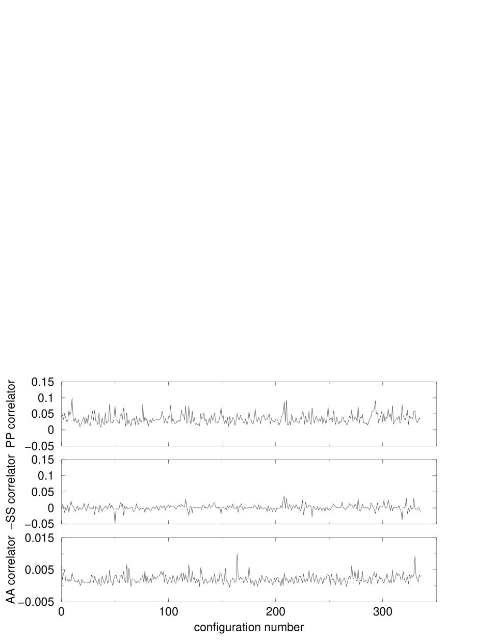
As a final step in demonstrating the zero mode effects in the various correlators, in Figure 17 the evolution of $\langle\pi^{a}(x)\pi^{a}(0)\rangle$, $\langle\sigma(x)\sigma(0)\rangle_{\rm c}$ and $\langle A_{0}^{a}(x)A_{0}^{a}(0)\rangle$ is shown for $8^{3}\times 32$ lattices at $\beta=5.7$ with $L_{s}=48$ and $m_{f}=0.0$. These correlators are from a point source to a point sink and the zero spatial momentum component is taken for the sink. The sink is at a separation $t=8$ from the source. The correlators $\langle\pi^{a}(x)\pi^{a}(0)\rangle$ and $-\langle\sigma(x)\sigma(0)\rangle_{\rm c}$ show very large fluctuations, which are common to both correlators, showing the presence of topological near-zero modes. These large fluctuations are clearly dominating the ensemble average for the correlators at this separation, $t=8$. The $\langle A_{0}^{a}(x)A_{0}^{a}(0)\rangle$ correlator does not show large fluctuations where $\langle\pi^{a}(x)\pi^{a}(0)\rangle$ and $\langle\sigma(x)\sigma(0)\rangle_{\rm c}$ do, making the topological near zero mode effects smaller for this correlator, as expected from the theoretical discussion of the previous subsection. Figure 18 is a similar plot, for the same configurations, except with $m_{f}=0.04$. There is no evidence for a large role being played by the topological near-zero modes.

Similar results have been obtained for simulations on $16^{3}\times 32$ lattices at $\beta=6.0$ with $L_{s}=16$. These lattices have essentially the same spatial volume, in physical units, as the previous $8^{3}\times 32$, $\beta=5.7$ lattices since the lattice spacing is half that for $\beta=5.7$. Figure 19 shows $m_{\pi}^{2}$ for $\langle A_{0}^{a}(x)A_{0}^{a}(0)\rangle$, $\langle\pi^{a}(x)\pi^{a}(0)\rangle$ and $\langle\pi^{a}(x)\pi^{a}(0)\rangle+\langle\sigma(x)\sigma(0)\rangle_{\rm c}$. For the smallest $m_{f}$ points, 0.0 and 0.001, all three correlators give different results. For larger values of $m_{f}$, the pion mass from $\langle A_{0}^{a}(x)A_{0}^{a}(0)\rangle$ and $\langle\pi^{a}(x)\pi^{a}(0)\rangle$ agree, while the $\langle\pi^{a}(x)\pi^{a}(0)\rangle+\langle\sigma(x)\sigma(0)\rangle_{\rm c}$ pion mass is systematically high, likely due to the contribution of the heavy states in $\langle\sigma(x)\sigma(0)\rangle_{\rm c}$. The lines drawn in Figure 19 are from correlated linear fits to $m_{\pi}^{2}$ using $m_{f}=0.01$ to 0.04. The dotted line is for $m_{\pi}^{2}$ from $\langle\pi^{a}(x)\pi^{a}(0)\rangle$, the solid line for $\langle A_{0}^{a}(x)A_{0}^{a}(0)\rangle$ and the dashed line for $\langle\pi^{a}(x)\pi^{a}(0)\rangle+\langle\sigma(x)\sigma(0)\rangle_{\rm c}$. The fit results are

$$m_{\pi}^{2}=0.0132(20)+3.07(6)m_{f} \chi^{2}/{\rm dof}=5.0\pm 5.0$$ (79)

$$m_{\pi}^{2}=0.0098(20)+3.14(9)m_{f} \chi^{2}/{\rm dof}=0.03\pm 0.30$$ (80)

$$m_{\pi}^{2}=0.0020(26)+3.56(8)m_{f} \chi^{2}/{\rm dof}=0.06\pm 0.51$$ (81)

for $\langle\pi^{a}(x)\pi^{a}(0)\rangle$, $\langle A_{0}^{a}(x)A_{0}^{a}(0)\rangle$ and $\langle\pi^{a}(x)\pi^{a}(0)\rangle+\langle\sigma(x)\sigma(0)\rangle_{\rm c}$ respectively.

Figure 20 shows effective mass plots for the pion from the three correlators for $m_{f}=0.001$ and Figure 21 is for $m_{f}=0.01$. Both figures show reasonable plateaus, even though there are differences in the final fitted masses. We have also studied the evolution of the correlators at a fixed $t$ for these $\beta=6.0$ lattices and see clear topological near-zero mode effects as were seen at $\beta=5.7$.

Thus, investigating the chiral limit of domain wall fermions in quenched QCD by measuring the pion mass is made difficult by the presence of topological near-zero modes. One component in the somewhat large values of $m_{\pi}^{2}$ plotted in Fig. 14 is the effect of topological near zero modes. As can be seen by a comparison with Table XVI the results we find from the correlator $\langle A_{0}^{a}(x)A_{0}^{a}(0)\rangle$ for $m_{\pi}^{2}(m_{f}=0)$ are about 1 1/2 standard deviations lower for $L_{s}=32$ and $48$. This is likely a systematic bias caused by the greater influence of the topological near-zero modes on the $\langle\pi^{a}(x)\pi^{a}(0)\rangle$ correlator. Unfortunately, these effects may also enter in the other correlators that can give $m_{\pi}$, at least for the source-sink time separations currently accessible. With this large distortion due to the topological near-zero modes, there we cannot determine the chiral limit by extrapolating to the point where $m_{\pi}^{2}$ vanishes. Subtler finite volume effects and possible quenched chiral logarithms are completely overshadowed by the singular nature of the basic quark propagators for small $m_{f}$.

In many ways, the presence of these topological near-zero modes is a welcome change from other lattice fermion formulations because they are a vital part of the spectrum of any continuum Dirac operator. However, in order to further investigate the chiral limit, they must be removed, or at least suppressed. Without adding the fermionic determinant to the path integral, we can suppress the effect of topological near-zero modes by going to large volumes.

C The pion mass for larger volume

Having seen clear evidence for topological near-zero modes in the measurements of the pion mass for lattices with a physical size of $\sim 2$ Fermi, we have worked on a larger physical volume, $\sim 4$ Fermi, to suppress the effects of these modes. As we saw in Section IV from studying $\langle\overline{q}q\rangle$, the effects of the topological near-zero modes were dramatically reduced for larger volumes. Here we present results for the pion mass from simulating with $16^{3}\times 32$ lattices at $\beta=5.7$ and $L_{s}=48$.

Figure 3 shows $m_{\pi}^{2}$ plotted against $m_{f}$ for these runs. In contrast to the smaller volume $8^{3}\times 32$ result shown in Figure 2, all three correlators now give the same results for the pion mass, within statistics (Table XXI). The larger volume has clearly reduced the effects of the zero modes. Further evidence of the consistency of the mass from the three correlators is shown in Figure 22. Here, for each $m_{f}$, the average value of $m_{\pi}$ is calculated and then the deviation from that average, for each correlator, is plotted. For each $m_{f}$, $\langle A_{0}^{a}(x)A_{0}^{a}(0)\rangle$ is offset to the left and the $\langle\pi^{a}(x)\pi^{a}(0)\rangle+\langle\sigma(x)\sigma(0)\rangle_{\rm c}$ to the right for clarity.

Figure 23 shows the effective mass from each of the three correlators for $m_{f}=0$. In contrast to the smaller volume case, the effective masses have quite similar values and lead to the same fitted mass, within errors. As a last comparison with the small volume, Figure 24 shows the three correlators at a time separation of $t=8$ as a function of configuration number. Little if any effect of topological near-zero modes is seen. Thus, we conclude that this larger volume has suppressed these effects as expected.

Having established that a consistent pion mass can be determined from our fitting range, we discuss the result of linear fits of $m_{\pi}^{2}$ as a function of $m_{f}$. We have done correlated linear fits of $m_{\pi}^{2}$ to $m_{f}$ for each of the correlators, using a variety of different ranges for $m_{f}$ in the fit. The resulting $\chi^{2}$ per degree of freedom is shown in Figure 25, including the jackknife error on the $\chi^{2}$. (The plotted error bars are the $\pm 1\sigma$ errors from the jackknife procedure and do not mean that $\chi^{2}$ can become negative.) The pion propagator for $m_{f}=0.0$ and 0.04 was measured on the same set of configurations, with some of the $m_{f}=0.08$ propagators also measured on those configurations. The $m_{f}=0.02$, 0.06 and 0.10 points were all measured on the same configurations, along with the remaining 0.08 propagators. Thus, these points are less correlated in $m_{f}$ than the corresponding measurements on the smaller volumes.

Now let us discuss the quality of these fits. Given the significant upward curvature of $m_{\pi}^{2}$ for $m_{f}\geq 0.1$, seen for example in Figure 2, we limit the mass range to $m_{f}\leq 0.08$. If we do not include the lightest masses and fit the points with $0.02\leq m_{f}\leq 0.08$, as shown in Figure 25 we obtain acceptable values for $\chi^{2}$ per degree of freedom for all three correlators. Specifically using the mass range $m_{f}=0.02$ to 0.08, the fits to $m_{\pi}^{2}$ from the correlators $\langle\pi^{a}(x)\pi^{a}(0)\rangle$, $\langle A_{0}^{a}(x)A_{0}^{a}(0)\rangle$ and $\langle\pi^{a}(x)\pi^{a}(0)\rangle+\langle\sigma(x)\sigma(0)\rangle_{\rm c}$ are

$$\begin{array}[]{cc}m_{\pi}^{2}=0.044(5)+4.75(5)m_{f}&\chi^{2}/{\rm dof}=1.4\pm 3.6\\ m_{\pi}^{2}=0.051(3)+4.68(4)m_{f}&\chi^{2}/{\rm dof}=1.4\pm 1.4\\ m_{\pi}^{2}=0.049(3)+4.70(5)m_{f}&\chi^{2}/{\rm dof}=2.5\pm 2.4.\\ \end{array}$$ (82)

However, given our confidence that this larger $16^{3}$ volume permits the reliable calculation of the pion mass for smaller values of $m_{\pi}$ we can also attempt a linear fit in the entire range $0.0\leq m_{f}\leq 0.08$. For this mass range, we find

$$\begin{array}[]{ccl}m_{\pi}^{2}=0.042(3)+4.77(3)m_{f}&\chi^{2}/{\rm dof}=1.3\pm 3.5\\ m_{\pi}^{2}=0.044(3)+4.75(5)m_{f}&\chi^{2}/{\rm dof}=4.3\pm 2.6\\ m_{\pi}^{2}=0.042(4)+4.82(6)m_{f}&\chi^{2}/{\rm dof}=4.4\pm 3.0\end{array}$$ (83)

for the correlators $\langle\pi^{a}(x)\pi^{a}(0)\rangle$, $\langle A_{0}^{a}(x)A_{0}^{a}(0)\rangle$ and $\langle\pi^{a}(x)\pi^{a}(0)\rangle+\langle\sigma(x)\sigma(0)\rangle_{\rm c}$ respectively. The $\langle A_{0}^{a}(x)A_{0}^{a}(0)\rangle$ and $\langle\pi^{a}(x)\pi^{a}(0)\rangle+\langle\sigma(x)\sigma(0)\rangle_{\rm c}$ fits suggest that $m_{\pi}^{2}$ is not linear in this mass range. While the $\langle\pi^{a}(x)\pi^{a}(0)\rangle$ fit is acceptable, as can be seen from a careful examination of Figure 3, this acceptable fit comes because the $m_{f}=0.02$ point lies somewhat below while the $m_{f}=0.0$ lies somewhat above the masses obtained from the other two correlators. Since the smaller volume studies suggest that the $\langle\pi^{a}(x)\pi^{a}(0)\rangle$ correlator is most sensitive to zero modes and such an upturn for small mass is the effect of zero modes seen at smaller volume, this could easily be a remaining zero mode distortion.

It is difficult to draw a firm conclusion from the relatively large correlated $\chi^{2}$/dof presented in Eq. 83. As is indicated by the errors shown, these $\chi^{2}$/dof are not reliably known. However, the comparison of the $\chi^{2}$/dof between Eqs. 82 and 83 may be more meaningful. We attribute significant weight to the fact that the lightest $m_{f}=0$ point lies below the value predicted by a linear extrapolation from larger masses as can be easily seen in Figure 3.

We conclude that a linear fit does not well represent our data over the full mass range $m_{f}=0.0$ to 0.1. Of course, non-linearities for larger masses can come from a variety of sources including terms from the naive analytic expansion in powers of $m_{f}$. However, for small $m_{f}$, linearity is expected for large volumes in full QCD. In contrast, in the quenched approximation the absence of the fermion determinant may result in complex and more singular infrared behavior. For example, it has been argued that a quenched chiral logarithm can appear in $m_{\pi}^{2}$ versus $m_{f}$ for quenched QCD [68, 69, 70]. The results just presented may be evidence for some non-linear behavior of this sort.

Because of the poor linear fits found for small $m_{f}$, our data does not allow a determination of the location of the chiral limit for quenched domain wall fermions by a simple extrapolation of $m_{\pi}^{2}$. Even with the suppression of topological near-zero mode effects that has been achieved by going to larger volume, further theoretical input may needed if we are to deduce $m_{\rm res}$ from these measurements of $m_{\pi}^{2}$. In the next section we will discuss our determination of the location of the chiral limit using other techniques and then return to the question of the behavior of $m_{\pi}^{2}$ with $m_{f}$.

VI The residual mass

A Determining the residual mass

In this section, we discuss our determination of $m_{\rm res}$ using the low-momentum identity in Eq. 15. This can done by calculating the ratio

$$R(t)=\frac{\langle\sum_{\vec{x}}J^{a}_{5q}(\vec{x},t)\pi^{a}(0)\rangle}{\langle\sum_{\vec{x}}J^{a}_{5}(\vec{x},t)\pi^{a}(0)\rangle}$$ (84)

as a function of $t$ (no sum on $a$), where $\pi^{a}(0)$ is a source evaluated at $t=0$ but possibly extended in spatial position. This ratio was first used to determine $m_{\rm res}$ in Ref. [10] and later in Refs. [29, 30]. Our results are consistent with this earlier work, but a much more detailed study is undertaken here. For $t$ outside some short-distance region, $t\geq t_{\rm min}$, $R(t)$ should be simply equal to $m_{\rm res}$. Using $R(t)$ for very large $t$ gives $m_{\rm res}$ as the coupling of the pion to the mid-point pseudoscalar density divided by its coupling to the wall pseudoscalar density. Of course, $m_{\rm res}$ is an additive contribution to the effective quark mass at low energies which effects all low-energy physics, not just the pion. To understand how large $t$ must be, Figure 26 shows a typical good plateau and a poor one. Results are shown for $8^{3}\times 32$ lattices with $m_{f}=0.04$ and $\beta=5.7$ for $L_{s}=32$ and 48. The good plateau is obtained from 335 configurations for $L_{s}=48$, while the poor plateau is obtained from 184 configurations for $L_{s}=32$. The fewer measurements for $L_{s}=32$ likely is the cause for the upturn in the data at large $t$ and adding more configurations at this $L_{s}$ should improve the signal.

From observing the onset of the plateaus in our data, we calculate $m_{\rm res}$ from the ratio in Eq. 84 using the range $4\leq t\leq 16$ for $\beta=5.7$, $6\leq t\leq 26$ for $\beta=5.85$, and $2\leq t\leq 16$ for $\beta=6.0$. The jackknife method is used to measure the statistical uncertainty and our $m_{\rm res}$ results at $\beta=5.7,5.85$ and $6.0$ are listed in Tables XXII and XXIII. For most data sets, nice plateaus can be seen over the selected range, while for the few others with the poor plateaus, using a different range could change the results by $<5\%$. We have also measured $m_{\rm res}$ for different values of $m_{f}$ for $\beta=5.7$ on $16^{3}\times 32$ lattices with $L_{s}=48$. Table XXIII gives the results and shows that the residual mass has little dependence on the input quark mass, reflecting the expected universal character of $m_{\rm res}$. Our $\beta=6.0$ results for $m_{\rm res}$ appear to be a consistent extension of the values plotted in Figure 5 of Ref. [30] for $L_{s}=4$, 6 and 10.

The $L_{s}$ dependence of $m_{\rm res}$ is of vital importance to numerical simulations with domain wall fermions. Without the effects of topological near-zero modes, quenched chiral logs and finite volume, $m_{\pi}^{2}(m_{f}=0)$ should be proportional to $m_{\rm res}$ and should vanish with $m_{\rm res}$ as $L_{s}\rightarrow\infty$. However, in Section V we discussed how topological near-zero mode effects alter $\langle\pi^{a}(x)\pi^{a}(0)\rangle$ and can distort the value of $m_{\pi}^{2}(m_{f}=0)$ for large $L_{s}$ shown in Figure 14. By measuring the ratio in Eq. 84, we can determine $m_{\rm res}$ for non-zero $m_{f}$ and suppress all these effects which make the $m_{f}\rightarrow 0$ limit problematic. This allows us to study the $L_{s}$ dependence of $m_{\rm res}$, to which we now turn.

From the two values of $L_{s}$ shown in Figure 26, we see that the residual mass for $8^{3}\times 32$ lattices at $\beta=5.7$ falls from $0.0105(2)$ to $0.00688(13)$ as $L_{s}$ is increased from $32$ to $48$. This is in sharp contrast to the almost identical results for $m_{\pi}^{2}(m_{f}=0)$ at these two values for $L_{s}$ (Figure 14). The overlap of the surface states is significantly suppressed, as expected, even at this relatively strong coupling. We have not pursued the asymptotic behavior for large $L_{s}$ at $\beta=5.7$, due to the large values for $L_{s}$ required, but instead have studied this question for $\beta=6.0$.

Figure 4 shows a similar study of the $L_{s}$ dependence of the residual mass for $16^{3}\times 32$ lattices with $m_{f}=0.02$ and $\beta=6.0$. The number of configurations used is modest for the larger values of $L_{s}$. We have used the factor $Z_{S}({\rm\overline{MS},2GeV})=0.619(25)$ obtained by a combination of non-perturbative renormalization and standard perturbation theory [72, 73] to convert the plotted values of $m_{\rm res}$ into MeV. The value of $m_{\rm res}$ is decreasing with $L_{s}$ for all values of $L_{s}$, but is poorly fit by a simple exponential. In particular, an exponential fit using all values of $L_{s}$ gives

$$m_{\rm res}=0.0068(4)\exp(-0.094(4)L_{s}),\ \ \ \chi^{2}/{\rm dof}(3)=32$$ (85)

which clearly does not match the measured values. Adding a constant to the fit gives

$$m_{\rm res}=0.00032(3)+0.018(3)\ {\rm exp}(-0.181(13)L_{s}),\ \ \ \chi^{2}/{\rm dof}(2)=4.1$$ (86)

where again all values for $L_{s}$ were used. Even if this is the correct asymptotic form, the value of $m_{\rm res}$ for $L_{s}\rightarrow\infty$ is very small, 1 MeV.

We have also tried fitting the largest three $L_{s}$ points to a simple exponential and find

$$m_{\rm res}=0.0012(2)\ {\rm exp}(-0.032(6)L_{s}),\ \ \ \chi^{2}/{\rm dof}(1)=0.074.$$ (87)

Our data is consistent with the residual mixing vanishing exponentially as $L_{s}\rightarrow\infty$, but the 0.032 coefficient in the exponent of Eq. 87 is quite small. Of course, we can easily obtain an excellent fit to our five points if we include a second exponential. For example, as shown in the figure, the five points fit well to two-exponential function

$$m_{\rm res}=0.038(16)\ {\rm exp}(-0.26(4)L_{s})+0.0010(3)\ {\rm exp}(-0.027(7)L_{s}),\ \ \ \chi^{2}/{\rm dof}(1)=0.1.$$ (88)

Our measurements do not demonstrate a precise asymptotic form for $m_{\rm res}$ as a function of $L_{s}$. However, we do see $m_{\rm res}$ decreasing for large $L_{s}$ until, for $L_{s}\geq 24$, it has become so small as to be essentially negligible for current numerical work. For $\beta=5.7$ at $L_{s}$ = 48, $m_{\rm res}$ is $0.074(5)$ in units of the strange quark mass, while for $\beta=6.0$ at $L_{s}=16$ it is $0.033(3)m_{s}$. In the latter case, where we know the renormalization factors, $m_{\rm res}$ in the $\overline{\rm MS}$ scheme at 2 GeV is 3.87(16) MeV. Thus, even though more simulations will be needed to get the precise asymptotic form, we find domain wall fermions having the expected chiral properties for large $L_{s}$, even for lattice spacings of around 1 Fermi.

In the next subsection, we will use the values of $m_{\rm res}$ that have just been determined to investigate further the $m_{f}$ dependence of $m_{\pi}^{2}$, looking in particular at possible non-linear behavior as $m_{f}+m_{\rm res}\rightarrow 0$. Here we would like to discuss a simpler consistency check on the values of $m_{\rm res}$ just obtained. For the $\pi$, $\rho$ and nucleon we have established good linear $m_{f}$ behavior for larger values of $m_{f}$ with slopes and intercepts given in Tables XVI and XVII. If the only effect on these masses of changing $L_{s}$ is to change the effective quark mass through the corresponding change in $m_{\rm res}$, then we should be able to relate the the differences in the intercepts given in these tables to the product of the corresponding slope times the change in $m_{\rm res}$ given in Tables  XXII and XXIII.

While this comparison shows no inconsistencies, the errors in the intercepts are typically too large to permit a detailed confirmation. For example, the difference in intercepts for $m_{\pi}^{2}$ at $\beta=6.0$ between $L_{s}=16$ and 24 is 0.0004(30) while the difference predicted from the slope and the measured change in $m_{\rm res}$ is 0.0020(2). The best test of this sort can be made using the actual value for $m_{\pi}$ determined at $\beta=5.7$ and $m_{f}=0.04$ for $L_{s}=32$ and 48. Here the difference of the masses squared is 0.012(6) while the prediction from the slope and change in $m_{\rm res}$ is 0.0176(12). Thus, we can demonstrate consistency with the expected behavior but cannot make a definitive test.

B The residual mass and $m_{\pi}^{2}$ versus $m_{f}$

The definition of $m_{\rm res}$ and its measurement mean that we have determined the value of $m_{f}$ for which the pion should become massless if the domain wall method is successfully representing the chiral limit of the underlying theory. We can now return to the question of the dependence of $m_{\pi}^{2}$ on $m_{f}$, starting with the $16^{3}\times 32$ simulations at $\beta=5.7$ and $L_{s}=48$. Recalling Figure 3, we found that the larger volume gave consistent pion mass measurements from the three correlators, but $m_{\pi}^{2}$ was not well fit as a linear function of $m_{f}$ for two of the correlators if the $m_{f}=0.0$ point was included. In Figure 3, we have included the value of $m_{\rm res}$ (the starred point) as measured from Eq. 84. (Its error bar on the horizontal axis is a vertical line on this scale.) The solid line is the fit to the $\langle A_{0}^{a}(x)A_{0}^{a}(0)\rangle$ correlator for $m_{f}=0.02$ to 0.08 given in Eq. 82 while the dotted line is for the $\langle\pi^{a}(x)\pi^{a}(0)\rangle$ correlator for $m_{f}=0.0$ to 0.08 as given in Eq. 83. Thus, we see that linear fits poorly represent the data when the $m_{f}=0.0$ point is included for the $\langle A_{0}^{a}(x)A_{0}^{a}(0)\rangle$ and $\langle\pi^{a}(x)\pi^{a}(0)\rangle+\langle\sigma(x)\sigma(0)\rangle_{\rm c}$ case and fail for all three correlators when the pion mass is required to vanish at $m_{f}=-m_{\rm res}$.

We can make this conclusion more quantitative by comparing our accurate value for $m_{\rm res}=0.00688(13)$ at $L_{s}=48$ determined on an $8^{3}\times 32$ lattice with the naive linear extrapolation of $m_{\pi}^{2}(m_{f})$ to the point $m_{\pi}^{2}=0$. Using the most reliable linear fits obtained by excluding the $m_{f}=0$ point in Eq. 82 we obtain the $x$-intercept values shown in Table XXIV: -0.0092(12), -0.0108(7) and -0.0104(7) for the $\langle\pi^{a}(x)\pi^{a}(0)\rangle$, $\langle A_{0}^{a}(x)A_{0}^{a}(0)\rangle$ and $\langle\pi^{a}(x)\pi^{a}(0)\rangle+\langle\sigma(x)\sigma(0)\rangle_{\rm c}$ correlators respectively. These differ from this value of $m_{\rm res}$ by $\approx 50\%$ and 2, 5 and 6 standard deviations respectively. We conclude that there is a significant discrepancy between the $m_{f}$-dependence of these $m_{\pi}$ results and the hypothesis that $m_{\pi}^{2}(-m_{\rm res})=0$. However, notice that if the $m_{f}=0$ points are included in the linear fits, and the less accurate $m_{\rm res}$ from the same volume is used, this discrepancy can be reduced. For example, a linear fit to the data from the $\langle\pi^{a}(x)\pi^{a}(0)\rangle$ correlator in Eq. 83 has an intercept at -0.0088(5) while $-m_{\rm res}=-0.0072(9)$ on the same volume. We believe that such an interpretation should be discounted as failing to exploit all the available information.

Is this significant discrepancy caused by essential non-linearities in the quenched approximation or by a breakdown of the domain wall method, for example, large $O(a^{2})$ effects? We can address this question by making a similar comparison for $\beta=6.0$ where $O(a^{2})$ effects should be significantly reduced. Since we have not investigated a large volume at this weaker coupling, we propose to examine the $\langle A_{0}^{a}(x)A_{0}^{a}(0)\rangle$ correlator because reduced zero-mode effects were seen for this correlator in our $\beta=5.7$ studies. Using the three lightest masses we find $x$-intercepts of -0.0031(7) and -0.0030(9) for the $L_{s}=16$ and 24 cases respectively. Again, these are dramatically farther from the origin than the corresponding values of $m_{\rm res}=0.00124(5)$ and 0.00059(4). These are each three standard deviation effects. However, they are obtained on independent configurations and together can be viewed as a 6 standard deviation discrepancy. Thus, if possible finite-volume difficulties are ignored, we have again strong evidence for a discrepancy. Rather than decreasing by a factor of four as would be expected from an $O(a^{2})$ error, this fractional discrepancy is substantially larger in this $\beta=6.0$ comparison. Thus, it is natural to conclude that domain wall fermions are accurately representing the chiral behavior of quenched QCD.

At the beginning of Section V we listed possible systematic effects influencing the chiral limit for $m_{\pi}$. With a measurement of $m_{\rm res}$ we have quantified the role of finite $L_{s}$ and with the larger volume used for $\beta=5.7$ we have reduced, if not eliminated the topological near-zero modes. We should also have minimized other finite volume distortions of the density of eigenvalues, which also influence the pion mass. Finally with the comparison above, we have examined the possibility of $O(a^{2})$ errors. Thus, we now address the question of quenched chiral logarithms. Predictions of this particular pathology of quenched simulations were made some time ago. There is certainly much data indicating possible support for the predictions, but there is disagreement about its conclusiveness, see for example refs. [74, 75, 76, 77, 78, 79]. Since many other effects must be removed before these subtle logarithms are convincingly seen, it is a challenging numerical issue.

The natural first place to look for quenched chiral logarithm effects is in $m_{\pi}$, but this is difficult for Wilson fermions, where the chiral point is not crisply defined for finite lattice spacing. For staggered fermions, where the chiral limit occurs when the input quark mass is zero, the issue is complicated by the presence of only a single Goldstone pion. In some respects, domain wall fermions are an ideal place to look for these effects, except that the statistical resolution needed is difficult to achieve with the additional computational load of the fifth dimension. In addition, the topological near-zero modes are a much larger quenched pathology at moderate volumes.

As one way of probing the non-linearity in $m_{\pi}^{2}$ versus $m_{f}$, we have fitted our data for $m_{\pi}^{2}$ for $16^{3}\times 32$ lattices at $\beta=5.7$ and $L_{s}=48$ to the form [68, 69, 70]

$$m_{\pi}^{2}=a_{0}(m_{f}+a_{1})(1+a_{2}\ln(m_{f}+a_{1}))$$ (89)

and the results are given in Table XXIV. The fit yields a value for the residual mass (the parameter $a_{1}$ above) and the results are quite close to those measured from the ratio of Eq. 84. Figure 27 shows the result from fitting $\langle A_{0}^{a}(x)A_{0}^{a}(0)\rangle$ for $m_{f}=0.0$ to 0.08 to the quenched chiral logarithm form given in Eq. 89. We have excluded the larger values of $m_{f}$ from our fits, since higher order terms are needed in Eq. 89 to accommodate the upward curvature of our $m_{\pi}^{2}$ data. While the $\chi^{2}$/dof for the logarithmic fit is only marginally better than those obtained for the simple linear fits described earlier in Eq. 83 for this same mass range, the ability of the logarithmic fit to predict the appropriate $m_{\rm res}$ value is significant.

For the simulations at smaller physical volumes, $8^{3}\times 32$ at $\beta=5.7$ and $16^{3}\times 32$ at $\beta=6.0$, the values for $m_{\rm res}$ measured from Eq. 84 are generally smaller than the $x$ intercepts for the linear fits shown in Figures 2 and 19. This indicates curvature in the direction given by a chiral logarithm, but the other phenomena that may be affecting these chiral limits make quantitative analysis ambiguous. We note that $m_{\pi}^{2}$ from $\langle\pi^{a}(x)\pi^{a}(0)\rangle+\langle\sigma(x)\sigma(0)\rangle_{\rm c}$ seems to smoothly curve towards the value of $m_{\rm res}$ from the previous subsection. However, we are not sufficiently certain of the absence of zero mode effects in the $\langle\pi^{a}(x)\pi^{a}(0)\rangle+\langle\sigma(x)\sigma(0)\rangle_{\rm c}$ correlator to describe a logarithmic fit to these cases.

This nice agreement between the values of $m_{\rm res}$ determined from the location of the $m_{\pi}^{2}=0$ point in these fits and that computed by other means earlier in the paper implies consistency between our results and the logarithmic form of Eq. 89. Of course, other non-linear terms could be used to explain this curvature and, given our statistics, would provide an equally consistent description of our data.

However, our most important conclusion is not related to quenched chiral logarithms, but rather to having seen all the expected properties for the chiral limit with domain wall fermions. Once the topological near-zero mode effects are reduced or eliminated, consistent pion masses can be measured. A precise measurement of $m_{\rm res}$ is consistent with our $m_{\pi}^{2}$ versus $m_{f}$ dependence if, for example, a chiral logarithm term is included. In short, domain wall fermions are showing sensible chiral properties, even on lattices with a lattice spacing of $\sim 1$ Fermi.

We have chosen not to pursue an additional method of determining $m_{\rm res}$ that has been proposed in two of our previous publications [25, 12]. In that method, one examines the integrated Ward-Takahashi identity in Eq. 60 and uses the location of the pion pole in $\chi_{\pi\pi}$ to determine $m_{\rm res}$. While this technique should be reliable for dynamical fermion calculations, e.g. as used in Ref [12], it does not explicitly allow for the effects of topological near-zero modes or possible non-linear behavior of $m_{\pi}^{2}(m_{f})$ that we have found to be important in the quenched approximation. Thus, even though this method gave a result for $\beta=5.7$ quite close [25] to the $L_{s}=48$ value $m_{\rm res}=0.00688(13)$ presented in this paper, more analysis is needed to adequately justify its use in this quenched case.

C Eigenvalue properties and $m_{\rm res}$

A comparison of the approximate form of the Banks-Casher relation for domain wall fermions given in Eq. 54 with the usual 4-dimensional expression in Eq. 44 suggests a close relationship between the parameter $\delta m_{i}$ deduced from the $i^{th}$ eigenvalue $\Lambda_{H,i}$ of $D_{H}$ and the residual mass $m_{\rm res}$. In this section we will explore this relation further making use of an exploratory study of the low-lying spectrum of $D_{H}$ [80].

These eigenvalues were calculated for 32 configurations obtained at $\beta=6.0$ on a $16^{4}$ lattice with $L_{s}=16$ listed in Table II and beginning with an equilibrated configuration from an earlier run. We used the Kalkreuter-Simma [48] method to find the 19 lowest eigenvalues on each configuration. We apply this method to the positive matrix $D_{H}^{2}$, and then determine the eigenvectors and eigenvalues of $D_{H}$ by a final explicit diagonalization of $D_{H}$ in the subspace of the eigenvectors of $D_{H}^{2}$ just determined. The details of our application of this method and a more complete description of these results will be presented in a later publication [80].

While this method determines both the eigenvalues and eigenvectors, we have chosen to examine only the $s$-dependent, four-dimensional inner products:

$$\Gamma_{R/L}(s)_{i,j}=\sum_{x}\Psi^{\dagger}(x,s)_{\Lambda_{H,i}}P_{R/L}\Psi(x,s)_{\Lambda_{H,j}},$$ (90)

where the indices $i,j$ run over all of the 19 eigenvalues while $P_{R}$ and $P_{L}$ are the left and right spin projection operators defined above Eq. 8. In order to be able to make use of the mass dependence of the eigenvalues, we have repeated the calculation of $\Lambda_{i}(m_{f})$ and $\Gamma_{R/L}(s,m_{f})_{i,j}$ five times on each configuration for the five different mass values $m_{f}=0.0$, 0.0025, 0.005, 0.0075 and 0.001.

Here we will describe some of the overall features of this calculation and then examine more closely the relation between the parameters $\delta m_{i}$ and the value of $m_{\rm res}$ determined earlier in this paper. First we examine the diagonal elements of the matrix $\Gamma(s)$

$${\cal N}(s)_{i}=\Gamma_{R}(s)_{i,i}+\Gamma_{L}(s)_{i,i}.$$ (91)

This is the contribution to the norm of the 5-dimensional wave function from the 4-dimensional hyperplane with a specific value of $s$. For these low lying eigenvalues, we expect that this norm should be concentrated on the $s=0$ and $s=L_{s}-1$ walls, which we find to be true to good accuracy. For the entire group of $32\times 19\ \times 5=3,040$ eigenvectors computed, the ratio of the sum of the norm on the two walls to the minimum value of this norm between the walls was always greater than 34, ${\cal N}(0)+{\cal N}(L_{s}-1)>34\cdot{\cal N}(s_{\rm min})$. The median value for this ratio was 744. Thus, the general framework upon which the domain wall formalism rests appears approximately valid.

As a test of our method for determining the eigenvectors, we evaluate the left- and right-hand side of the symmetry relation, Eq. 28, between pairs of eigenvectors on a given configuration. The resulting equality:

$$(\Lambda_{H,i}+\Lambda_{H,j})\langle\Lambda_{H,i}|\Gamma_{5}|\Lambda_{H,j}\rangle=\langle\Lambda_{H,i}|\Bigl{(}2m_{f}Q^{\rm(w)}+2Q^{\rm(mp)}\Bigr{)}|\Lambda_{H,j}\rangle$$ (92)

provides a good test of our diagonalization procedure. The vectors $|\Lambda_{H,j}\rangle$ needed to evaluate this expression are eigenvectors of the Dirac operator $D_{H}$, not $D_{H}^{2}$. We determine the eigenvectors of $D_{H}$ by diagonalization within the 19-dimensional subspace found by applying the Kalkreuter-Simma method to $D_{H}^{2}$. In the event that the $19^{th}$ and $20^{th}$ eigenvalues of $D_{H}^{2}$ are nearly degenerate (not entirely unlikely given the expectation that the eigenvalues of $D_{H}$ occur in $\pm\Lambda_{H}$ pairs), this truncated, 19-dimensional subspace will not be spanned by eigenvectors of $D_{H}$. It will contain 18 valid eigenvectors and a $19^{th}$ vector, orthogonal to the rest but not an eigenvector of $D_{H}$. This “spurious” eigenvector can be reliably removed since it will give an “eigenvalue” whose square does not agree with any found for $D_{H}^{2}$. We remove such eigenvectors from our test of Eq. 92 and, for uniformity, the $19^{th}$ eigenvector in the case that no spurious eigenvector occurs. There are then $32\times 5=160$ instances where we can check $18^{2}$ independent elements of Eq. 92. We find that 95% of these 51,840 comparisons have a fractional error below 5%. The few cases with significantly worse agreement, result from infrequent near degeneracies which challenge the Rayleigh-Ritz method on which the Kalkreuter-Simma algorithm is based.

For most configurations there are easily identified zero modes. Typically the few lowest eigenvalues have eigenvectors all of which are bound to the same wall, either $s=0$ or $s=L_{s}-1$. The corresponding matrix elements $\langle\Lambda_{H,i}|\Gamma_{5}|\Lambda_{H,i}\rangle$ all have the same sign and are within a few percent of 1, showing precisely the structure expected in a four-dimensional theory as summarized in Eq. 41.

The potential of the domain wall method is nicely displayed by examining the properties of one of our better configurations. In Fig 28, we show the magnitude of the elements of the matrix $\langle\Lambda_{H,i}|\Gamma_{5}|\Lambda_{H,j}\rangle$ in a three-dimensional plot. Note the five zero-modes in this configuration are easily recognized. Each has a diagonal matrix element of $\Gamma^{5}$ within 1.5% of 1 and matrix elements with other vectors all of magnitude below 0.06. The values of $\lambda_{i}$ for these five eigenvalues all lie in magnitude below $3.6\times 10^{-4}$ while the remaining paired eigenvalues lie between 0.028 and 0.093. In Figures 29 and 30 we show the $s$-dependence of the first two zero-modes and the first pair of non-zero eigenvectors, numbers 5 and 6. One sees precisely the expected behavior. Both zero-modes are bound to the same wall (as are the other three zero modes) while the two paired non-zero modes are nearly symmetrical between right and left. This is clearly identified as a configuration with topological charge $\nu=+5$.

Of direct interest in this section is the mass dependence of $\Lambda(m_{f})_{H,i}$ and a quadratic fit of the sort proposed in Eq. 51. For the small masses we have used, this quadratic form provides an excellent fit, after some re-sorting of eigenvalues is performed to account for infrequent level crossings as $m_{f}$ is varied. In order to avoid the possibility that these level crossings may have pushed a needed eigenvalue up to beyond number 19, we have excluded those quadratic fits which contain the largest eigenvalue at $m_{f}=0$ for each of the 32 configurations. The resulting root-mean-square of the fractional differences between the left- and right-hand sides of Eq. 51 is very small. The average root-mean-square of the fractional difference is $1.3\times 10^{-4}$ while the largest value is $4.3\times 10^{-3}$.

In Figure 31 we present a histogram of the distribution of fit parameters for the $18\times 32=576$, $\delta m_{i}$ values that we obtain. The majority of values are quite small, very much on the order of $m_{\rm res}$. While a few larger values of $\delta m_{i}$ are seen (the largest is 0.0660), the median of the distribution is $\overline{\delta m}=0.00147$ which is remarkably close to the value of $m_{\rm res}=0.00124$ found earlier for this value of $\beta$ and $L_{s}$.

The 4-dimensional expression for $\langle\overline{\psi}\psi\rangle$ in Eq. 44 and the 5-dimensional result in Eq. 54 as a function of $m=Zm_{f}$ must agree in the continuum limit after a rescaling and overall subtraction. This must be true even if $m_{\rm res}$ is held fixed in physical units as $a\rightarrow 0$. Therefore, in the limit of zero lattice spacing, the histogram shown in Figure 31 must approach a delta function so that $\delta m_{i}$ has the unique value $m_{\rm res}$. Thus, we might interpret the width of the distribution in Figure 31 as a result of $O(a^{2})$ effects. The large size of the fluctuations relative to the central value is presumably a result of the small central value produced by our quite large separation of 16 between the walls.

VII Hadronic Observables

We can now use the results of the previous sections to compute a variety of hadronic properties. In this section we will discuss two topics: the evaluation of the pion decay constant $f_{\pi}$ and the scaling properties of the nucleon to $\rho$ mass ratio. The first topic is of greatest interest since we can compute the pion decay constant using two independent methods, one of which depends directly on the residual mass determined in Section VI. The close agreement between these two approaches provides a very important consistency check of the analysis and results presented in this paper.

A Calculation of $f_{\pi}$

In the conventional continuum formulation, the pion decay constant $f_{\pi}$ is defined through the equation

$$\Big{\langle}0\Big{|}i\overline{\psi}\gamma^{\mu}_{M}\gamma_{5}t^{a}\psi\Big{|}\pi^{b}(\vec{p})\Big{\rangle}~{}\equiv~{}f_{\pi}{p^{\mu}\delta^{a,b}\over\sqrt{2E_{\pi}(\vec{p})}}$$ (93)

where the fields $\psi$ and $\overline{\psi}$ are interpreted as conventional, Hilbert space quark operators and the pion state obeys the non-covariant normalization $\langle\pi(\vec{p}\,^{\prime})|\pi(\vec{p})\rangle=\delta^{3}(\vec{p}-\vec{p}\,^{\prime})$. To be concrete we adopt the Minkowski metric $g^{\mu\nu}$ with signature $(-1,+1,+1,+1)$ and a Minkowski gamma matrix convention in which $\gamma^{0}_{M}$ is anti-hermitian and $\{\gamma^{\mu}_{M},\gamma^{\nu}_{M}\}=2g^{\mu\nu}$. With this normalization, $f_{\pi}\approx 130$ MeV.

Following the usual methods of lattice gauge theory, we evaluate matrix elements of the two-quark operator appearing in Eq. 93 with the Euclidean time dependence resulting from use of the evolution operator $e^{-Ht}$ where $H$ is the QCD Hamiltonian. Thus, we choose to evaluate

$$f_{\pi}^{2}{m_{\pi}\over 2}e^{-m_{\pi}t}=\lim_{T\rightarrow\infty}{Tr\Big{\{}e^{-H(T-t)}\;\int d^{3}x\;i\bar{\psi}\gamma^{0}_{M}\gamma_{5}t^{a}\psi(\vec{x},t)\;e^{-Ht}\;i\bar{\psi}\gamma^{0}_{M}\gamma_{5}t^{a}\psi(\vec{0},0)\Big{\}}\over Tr\big{\{}e^{-HT}\big{\}}}$$ (94)

where no sum over the flavor index $a$ is intended and the time $t$ is assumed sufficiently large that only the pion intermediate state contributes.

The continuum operators in Eq. 94 are easily represented as lattice, Euclidean-space expressions once the usual transition to a Euclidean-space path integral has been performed. In particular, the operators $\psi(\vec{x})$ and $\overline{\psi}(\vec{x})=\psi^{\dagger}(\vec{x})\gamma^{0}$ are replaced by the Grassmann variables $q(\vec{x},t)$ and $\overline{q}(\vec{x},t)$ respectively. Thus, we extract $f_{\pi}^{2}$ from the usual Euclidean correlation function:

$${f_{\pi}^{2}\over Z_{A}^{2}}{m_{\pi}\over 2}e^{-m_{\pi}t}=\Big{\langle}\int d^{3}x\;\overline{q}\gamma^{0}\gamma^{5}t^{a}q(\vec{x},t)\;\overline{q}\gamma^{0}\gamma^{5}t^{a}q(\vec{0},0)\Big{\rangle}$$ (95)

where now Euclidean gamma matrices appear, obeying $\{\gamma^{\mu},\gamma^{\nu}\}=2\delta^{\mu\nu}$. Here we have introduced the Grassmann variables $q$ and $\overline{q}$ defined earlier in this paper so the axial current appearing in Eq. 95 is explicitly constructed from the five-dimensional quark fields $\Psi$ and $\overline{\Psi}$ restricted to the $s=0$ and $s=L_{s}-1$ walls. This “local” current, $A_{\mu}^{a}$ is not conserved in the full five-dimensional theory so the factor $Z_{A}$ appearing on the left hand side of Eq. 95 is needed to make a connection to the continuum axial current.

The conserved current ${\cal A}^{a}_{\mu}$ defined in Eq. 8 must approach the corresponding, partially conserved continuum current with unit normalization, when the continuum limit is taken. Thus, to order $a^{2}$, the low energy matrix elements of ${\cal A}_{\mu}^{a}$ and $A_{\mu}^{a}$ must be proportional: ${\cal A}_{\mu}^{a}=Z_{A}A_{\mu}^{a}$. While we have computed $f_{\pi}$ using the local current $A_{\mu}^{a}$ we have also compared that current to the partially conserved domain wall axial current ${\cal A}_{\mu}^{a}$, allowing an accurate determination $Z_{A}$.

In addition to the procedure just described, there is a second, independent method that we have used to compute $f_{\pi}$. Here we use the Ward-Takahashi identity to relate ${\cal A}_{\mu}^{a}$ and the pseudo-scalar density $J^{a}_{5}$:

$$\Delta_{\mu}{\cal{A}}_{\mu}^{a}(x)\approx 2(m_{f}+m_{\rm res}){J}^{a}_{5}(x)$$ (96)

an expression valid for low energy matrix amplitudes . In particular, we have replaced the usual midpoint term in the exact identity of Eq. 10 by its low energy limit: $2m_{\rm res}J^{a}_{5}(x)$. Thus, we can also obtain $f_{\pi}$ from the correlation function:

$$-{f_{\pi}^{2}\over(m_{f}+m_{\rm res})^{2}}{m_{\pi}^{3}\over 8}e^{-m_{\pi}t}=\Big{\langle}\int d^{3}x\;\overline{q}\gamma^{5}t^{a}q(\vec{x},t)\;\overline{q}\gamma^{5}t^{a}q(\vec{0},0)\Big{\rangle}$$ (97)

where again no sum over the flavor index $a$ is intended. This formula involves no renormalization factors but requires knowledge of the residual mass $m_{\rm res}$ induced by mixing between the walls. Thus, a comparison of the values for $f_{\pi}$ obtained from Eqs. 95 and 97 provides a critical test of the analysis presented in this paper.

We will now discuss these two calculations of $f_{\pi}$ in detail. To measure the value for the renormalization factor $Z_{A}$, we compare the amplitudes of two-point functions $C(t)$ and $L(t)$ defined as

$$C(t+1/2) = \sum_{\vec{x}}\langle{\cal A}^{a}_{0}(\vec{x},t)\;\pi^{a}(\vec{0},0)\rangle$$ (98)

$$L(t) = \sum_{\vec{x}}\langle A^{a}_{0}(\vec{x},t)\;\pi^{a}(\vec{0},0)\rangle.$$ (99)

The $1/2$ in the argument of $C(t+1/2)$ in Eq. 99 comes from the fact the conserved axial current ${\cal A}^{a}_{\mu}(x)$ is not the current at lattice site $x$ but instead the current carried by the link between $x$ and $x+\hat{\mu}$. We take appropriate arithmetic averages to solve the problem that $C(t+1/2)$ and $L(t)$ are not at the same location. To avoid as much systematic error as possible, we define $Z_{A}(t)$ as

$$Z_{A}(t)=\frac{1}{2}\left\{\frac{C(t+1/2)+C(t-1/2)}{2\ L(t)}+\frac{2\ C(t+1/2)}{L(t)+L(t+1)}\right\}.$$ (100)

For $t\gg a^{-1}$, $C(t)/L(t)$ behaves like a constant which can be identified with $Z_{A}$. Both terms in Eq. 100 estimate this value without $O(a)$ error. The average of these two, incorporated in Eq. 100, further eliminates a portion of the $O(a^{2})$ error.

Figure 32 shows the ratio $Z_{A}(t)$ defined in Eq. 100 for both a $16^{3}\times 32$ lattice with $L_{s}=16$, and $\beta=6.0$ as well as the same quantity for a $8^{3}\times 32$ lattice with $L_{s}=48$ and $\beta=5.7$. We determine the value for the renormalization factor $Z_{A}$ by calculating the average over two ranges of $t$: $4\leq t\leq 14$ and $18\leq t\leq 28$, chosen to avoid the largest time separation $t\sim 16$ where the errors are quite large. A jackknife error is determined, to compensate for possible correlation between the numerator and denominator in Eq. 100.

The results for $Z_{A}$ at $\beta=6.0$, $16^{3}\times 32$, $M_{5}=1.8$ and with different values of $L_{s}$ are listed in Table XXV. The data shows little $L_{s}$ dependence, as should be expected. Figure 32, also shows our result of $Z_{A}=0.7732(14)$ found for the $8^{3}\times 32$ lattice with $\beta=5.7$, $L_{s}=48$, $M_{5}=1.65$, $m_{f}=0.02$.

The results for the amplitudes for the axial vector current correlator and the pseudoscalar density correlator at $\beta=5.7$ and $6.0$ are given in Tables XXVI-XXX. They are obtained from the point-source correlators using a conventional 2-parameter fit with the pion masses extracted concurrently. We also list in the same tables the results for $f_{\pi}$ as a function of $m_{f}$ determined from the corresponding correlators with the help of $Z_{A}$ and $m_{\rm res}$ (Tables XXII-XXIII). These values of $f_{\pi}$ have been converted to physical units using the measured $\rho$ mass discussed in Section III, extrapolated to the chiral limit $m_{f}+m_{\rm res}=0$.

Next, we use a linear fit in $m_{f}$ to evaluate $f_{\pi}$ for two values of $m_{f}$. To obtain a value of $f_{\pi}$ close to that for the physical pion, we go to the chiral limit $m_{f}+m_{\rm res}=0$. For $f_{K}$ we choose for $m_{f}$ that value which gives $m_{\pi}/m_{\rho}=0.645$. In determining $f_{\pi}$ for the physical pion state, we did not attempt to use a value of $m_{f}$ giving the physical value for the ratio $m_{\pi}/m_{\rho}=0.18$ since we do not adequately know the $m_{f}$ dependence of this ratio in the relevant region. These linear fit parameters as well as the resulting values for $f_{\pi}$ and $f_{K}$ are summarized in Table XXXI. The errors given in the tables are obtained from the jackknife method.

Figure 33 shows the values for $f_{\pi}$ at $\beta=5.7$, $8^{3}\times 32$, $L_{s}=48$ as a function of $m_{f}$ and the linear fits through all the $m_{f}$ points. The results obtained from the pseudoscalar-pseudoscalar correlator are higher than those from the axial-axial correlator. The two linear fits give $f_{\pi}=127(4)\ {\rm MeV}$, $f_{K}=145(4)\ {\rm MeV}$ and $f_{\pi}=132(4)\ {\rm MeV}$, $f_{K}=154(4)\ {\rm MeV}$ respectively. When the lattice volume is increased to $16^{3}\times 32$ (Figure 34), the difference between the linear fits from the two methods becomes smaller. We obtain $f_{\pi}=133(4)\ {\rm MeV}$, $f_{K}=149(2)\ {\rm MeV}$ and $f_{\pi}=125(4)\ {\rm MeV}$, $f_{K}=149(2)\ {\rm MeV}$ from the two correlators. The values for $f_{\pi}(m_{f})$ obtained from the two methods should agree for all values of $m_{f}$ since they are related by a Ward-Takahashi identity that should become exact in the continuum limit. Presumably the visibly different slopes seen in Figures 33 and 34 are the result of order $a^{2}$ errors.

We also calculate $f_{\pi}$ at a weaker coupling. Figure 5 shows our results for $\beta=6.0$, $16^{3}\times 32$, $L_{s}=16$ on 85 configurations. The two independent calculations give very consistent results. We have $f_{\pi}=137(11)\ {\rm MeV}$, $f_{K}=156(8)\ {\rm MeV}$ from the axial vector current correlator and almost the same values from the pseudoscalar correlator. Our results for $f_{\pi}$ at both $\beta=5.7$ and $6.0$ agree well with the experimental value of $\approx 130\ {\rm MeV}$, while the values for $f_{K}$ may be somewhat smaller than the experimental value of $\approx 160\ {\rm MeV}$ as is expected from quenched chiral perturbation theory arguments [69] and naive scaling considerations [81]. Note, in Table XXXI we also list $f_{K}/f_{\pi}$ with jackknifed errors for the ratio. Here the statistical errors are now well below the systematic errors that might be expected in the $m_{f}+m_{\rm res}\rightarrow 0$ extrapolation. The values shown for $f_{K}/f_{\pi}$ agree on the 5% level between methods of determination and different lattice spacings but are systematically below the experimental value of 1.21.

This same analysis was done using the amplitudes calculated from the point-source correlators but making a 1-parameter fit using the pre-determined pion masses computed from the more mass accurate measurements based on the wall-source correlators. This method gives consistent results with slightly smaller errors. The results are not listed here.

The reasonable agreement of our domain wall results with the experimental values and their relative insensitivity to $a$ is encouraging. Similar results were obtained at $\beta=6.0$ for smaller values of $L_{s}$ with somewhat larger errors in Ref. [30]. Of special interest here is the comparison that we make between the two methods of determining $f_{\pi}$, which is done here for the first time. As can be seen from Eq. 97, the determination of $f_{\pi}$ from $\langle\pi^{a}(x)\pi^{a}(0)\rangle$ depends directly on $m_{\rm res}$. Thus, the comparison of these two methods is an important check of our understanding of the chiral properties of the domain wall formulation. The ratio of these two quantities extrapolated to the point $m_{f}+m_{\rm res}=0$ provides an interesting figure of merit for the present calculation. We find $(f_{\pi})_{PP}/(f_{\pi})_{AA}=1.00(10)$ and 0.96(10) for $L_{s}=16$ and 24 respectively. However, if instead of the values of $m_{\rm res}$ given in Table XXII, we use the $x$-intercepts -0.0031(7) and -0.0030(9) quoted earlier and obtained from the $\langle A_{0}^{a}(x)A_{0}^{a}(0)\rangle$ values of $m_{\pi}^{2}$, we find $(f_{\pi})_{PP}/(f_{\pi})_{AA}=1.20(12)$ for both the $L_{s}=16$ and 24 cases. While these ratios each differ from 1 by two standard deviations, they are independent calculations and demonstrate the good chiral properties of domain wall fermions.

B Continuum limit of $m_{N}/m_{\rho}$

Here we combine the hadron mass results tabulated in Section III to examine the behavior of the nucleon to $\rho$ mass ratio as $\beta$ varies between 5.7 to 6.0. First we evaluate $m_{N}$ and $m_{\rho}$ in the limit $m_{f}+m_{\rm res}=0$. We did not use the value of $m_{f}$ which gives the physical ratio, $m_{\pi}/m_{\rho}=0.18$ for the reasons outlined in the previous section. In Table XXXII we give the resulting mass ratios as well as the lattice spacings in physical units as determined from $m_{\rho}$ evaluated at $m_{f}+m_{\rm res}=0$. Note, no contribution to the quoted error for these mass ratios arising from the uncertainty in this choice of $m_{f}$ has been included.

The relatively large variation of $m_{N}/m_{\rho}$ with $\beta$ suggests that the errors shown in Table XXXII may be underestimated and makes a simple $a^{2}$ extrapolation to the continuum limit somewhat uncertain. Nevertheless the result of such an extrapolation to $a\rightarrow 0$ is $m_{N}/m_{\rho}=1.37(5)$. Perhaps more interesting is a comparison with similar quantities computed at comparable lattice spacings and volumes using Wilson and staggered fermions. For staggered fermions at $\beta=6.0$ on comparable volumes, one finds [82, 83] $m_{N}/m_{\rho}=1.47(3)$, a somewhat larger and less physical value than the 1.42(4) and 1.38(4) results obtained here for $L_{s}=16$ and 24. However, this comparison is made somewhat ambiguous by the significant finite size effects seen in staggered calculations when going from our $16^{3}\times 32$ to larger volumes [84]. For Wilson fermions, as reported in Ref. [85], one deduces $m_{N}/m_{\rho}=1.37(2)$ by linear interpolation between the $\beta=5.93$ and 6.17 values presented, a number remarkably close to our domain wall value. When comparing these values, it is important to recall that our $8^{3}$ and $16^{3}$ spatial volumes are not yet infinite and, as discussed in Section III, corrections on the order of a few percent are expected.

C Determining the chiral condensate $\langle\overline{q}q\rangle$

Finally we use the results presented earlier to estimate the size of the chiral condensate $\langle\overline{q}q\rangle$. Naively, one might expect that a physical value for $\langle\overline{q}q\rangle$ could be easily identified in Table XX as the $m_{f}$-independent term $a_{0}$, defined in Eq. 55. This quantity represents a simple extrapolation of $\langle\overline{q}q\rangle(m_{f})$ from large mass down to the point $m_{f}=0$. Given the volume independence seen for the parameter $a_{0}$ when comparing the $\beta=5.7$, $8^{3}$ and $16^{3}$ volumes in Table XX, it is natural to expect that such a choice minimizes the sensitivity to the finite-volume zero mode effects that give rise to the more singular $a_{-1}$ term.

However, there are other issues that must be addressed. Perhaps most obvious is the fact that the point $m_{f}=0$ is not the physical chiral limit because the effects of $m_{\rm res}$ have been ignored. This is easily remedied by using the slope $a_{1}$, to extrapolate to the physical point $m_{f}+m_{\rm res}=0$. The resulting estimate of $\langle\overline{q}q\rangle$, in lattice units, is given as the fourth column in Table XXXIII. However, because $\langle\overline{q}q\rangle$ is a quadratically divergent quantity, we cannot expect that all the chiral symmetry breaking effects of domain wall mixing are removed by this choice of $m_{f}$. In contrast to many physical quantities, $\langle\overline{q}q\rangle$ receives contributions from energy scales much larger than those for which $m_{\rm res}$ represents the complete effect of chiral symmetry breaking. Thus, we should expect additional contributions to $\langle\overline{q}q\rangle$ of order $e^{-\alpha L_{s}}/a^{3}\sim m_{\rm res}/a^{2}$. This is born out in Table XXXIII where we see that the differences between $\langle\overline{q}q\rangle$ for the two different values of $L_{s}$ at a given $\beta$ are of the same order as the difference between the values with and without the extrapolation to $m_{f}=-m_{\rm res}$.

This unwanted $\sim m_{\rm res}/a^{2}$ contribution to $\langle\overline{q}q\rangle$ can only be controlled by explicitly taking the limit $L_{s}\rightarrow\infty$. We do not at present have the numerical results to permit such an extrapolation. Therefore, we will use the $\beta=6.0$, $L_{s}=24$ result as our best approximation to such a limit and interpret the difference between the $L_{s}=16$ and 24 values as an estimate of the systematic error, $\approx 10\%$. Given the value of $Z_{S}({\rm\overline{MS},2GeV})=0.619(25)$ for $\beta=6.0$ quoted earlier and the results for the lattice spacing in physical units in Table XXXII, we can determine $\langle\overline{q}q\rangle$ in physical units. The results for $L_{s}=16$ and 24, $(245(7){\rm MeV})^{3}$ and $(256(8){\rm MeV})^{3}$, are included in Table XXXIII, where only the statistical error is displayed. The agreement between these numbers and phenomenological estimates of the chiral condensate is satisfactory, for example the value of ${1\over 2}(\bar{u}u+\bar{d}d)_{\rm\overline{MS},1GeV}=(229\pm 9{\rm MeV})^{3}$ obtained in Ref. [86]. Note the $e^{-\alpha L_{s}}/a^{3}$ uncertainty present in our calculation does not have an analogue in the properly regulated continuum theory. While $\langle\overline{\psi}\psi\rangle$ does contain a quadratically divergent piece in the continuum theory, this is eliminated for the chirally symmetric choice $m_{\rm quark}=0$. This choice is not available in a domain wall fermion calculation without taking the $L_{s}\rightarrow\infty$ limit. Of course, the other lattice methods for directly computing $\langle\overline{\psi}\psi\rangle$ have equal or more severe difficulties.

Finally it is interesting to compare the $\beta=5.7$ and $\beta=6.0$ results for $\langle\overline{q}q\rangle$. Since we do not at present have a reliable determination of the needed renormalization constant, $Z_{S}$, for the stronger $\beta=5.7$ coupling, we do not attempt to quote a physical value. However, the ratio of the unrenormalized lattice numbers given in Table XXXIII for $\langle\overline{q}q\rangle_{(L_{s}=32,\,\beta=5.7)}/\langle\overline{q}q\rangle_{(L_{s}=24,\,\beta=6.0)}=4.8(2)$ is reasonably consistent with the ratio expected from naive scaling $a^{3}_{(L_{s}=32,\,\beta=5.7)}/a^{3}_{(L_{s}=24,\,\beta=6.0)}=7.4(4)$.

Given the values now determined for $\langle\overline{q}q\rangle$, $f_{\pi}$ and quark mass, it is natural to test the degree to which the Gell-Mann-Oakes-Renner relation [87]

$$f_{\pi}^{2}{m_{\pi}^{2}\over 48(m_{f}+m_{\rm res})}=-\langle\overline{q}q\rangle$$ (101)

is obeyed. However, the form of this equation reveals an important difficulty. At what value of $m_{f}$ should the ratio $m_{\pi}^{2}/(m_{f}+m_{\rm res})$ be computed? In full QCD, this ratio becomes a constant for small quark mass. As we have seen earlier, this is not the case in the quenched approximation where one expects non-linearities.

We might try to determine the proper treatment of these non-linearities by returning to the underlying equation, Eq. 60, from which the Gell-Mann-Oakes-Renner relation is derived. However, this is somewhat complex. Both sides of this original equation have a mass dependence which comes from the contribution of the pion pole term and other physical states, all influenced by the quenched approximation, as well as the quadratically divergent terms in $\langle\overline{q}q\rangle$ and the contact term in $\chi_{\pi\pi}$. Thus, while the underlying Eq. 60 will be obeyed exactly in our calculation, there is considerable ambiguity in deciding how to extract a quenched generalization of the Gell-Mann-Oakes-Renner relation, Eq. 101.

Here we will simply compare the right- and left-hand-sides of Eq. 101 by replacing the ratio $m_{\pi}^{2}/(m_{f}+m_{\rm res})$ by the slope $b$ obtained at larger masses, $m_{f}\geq 0.01$ and given in Tables XVI, XVII and XIX. The results from the left hand side of Eq. 101 are given in Table XXXIII. Given our uncertainty in determining $\langle\overline{q}q\rangle$ and the significant non-linearities we see in $m_{\pi}^{2}$, the agreement seen between the fourth and fifth columns in Table XXXIII is within our errors.

VIII Conclusions

We have presented the results of detailed studies of quenched lattice QCD using domain wall fermions, with particular attention paid to the lowest order chiral symmetry breaking effects of finite $L_{s}$ and the behavior of the theory for small values of $m_{f}$. A major difficulty in studying the small $m_{f}$ behavior of the theory is the presence of topological near-zero modes which are unsuppressed in the quenched theory. These are a result of the improved character of the domain wall fermion operator, which has an Atiyah-Singer index at finite lattice spacing and $L_{s}\rightarrow\infty$. However, these zero-modes complicate the quenched theory and demonstrate that the quenched approximation is considerably more treacherous than might have been originally expected. We have seen how these modes produce the expected $1/m_{f}$ divergence in $\langle\overline{q}q\rangle$ for small $m_{f}$ and distort correlation functions used to measure the properties of the pion. By working on larger volumes, we found that the effects of these modes were dramatically reduced, as expected. We were then able to see a common pion mass determined from different correlators.

We have determined or constrained the value for the residual mass, $m_{\rm res}$, which enters the effective quark mass for low-energy physics as $m_{\rm eff}=m_{f}+m_{\rm res}$, a number of ways and found good agreement. The residual mass was measured from the extra, finite $L_{s}$ term in the divergence of the conserved axial current and from the explicitly determined lowest eigenvalues of the hermitian domain wall fermion operator. These two determinations agree within errors. We have also determined the difference in $m_{\rm res}$ for two values of $L_{s}$ from the pion mass and find this agrees with the results from our explicitly calculated $m_{\rm res}$. Lastly, agreement for $f_{\pi}$ as calculated from axial vector and pseudoscalar correlators requires knowledge of $m_{\rm res}$ and the agreement serves as a further check.

While our data for weaker couplings does not clearly demonstrate that $m_{\rm res}\rightarrow 0$, we have seen it fall to 1 MeV for $L_{s}=48$ at $\beta=6.0$. For $L_{s}=16$, a practical value for studies of low energy hadronic physics and matrix elements, $m_{\rm res}$ has a value of 3.87(16) MeV, roughly 1/30 of the strange quark mass. Even at stronger couplings, where the lattice spacing is $a^{-1}\sim 1$ GeV, we have measured $m_{\rm res}$ to also be about 1/14 of the strange quark mass, although here $L_{s}=48$ was required. Thus, we see domain wall fermions producing the desired light surface states with small mixing, even for relatively strong couplings.

We have measured hadron masses and $f_{\pi}$ for lattice scales 1 GeV $<a^{-1}<$ 2 GeV and have studied scaling in this region. Our determinations of $f_{\pi}$ involve not only $m_{\rm res}$ as mentioned above but also the measurement of the Z-factor for the local axial current. We find $f_{\pi}/m_{\rho}$ evaluated at the $m_{f}+m_{\rm res}=0$ point to be scaling very well, while for $m_{N}/m_{\rho}$ the scaling violations may be at the 6% level. However, scaling seems at least as good as that seen for staggered fermions at similar lattice spacings and similar to that found for Wilson fermions with a clover term [84]. This is in accord with general expectations that finite lattice spacing errors will enter domain wall fermion amplitudes at $O(a^{2})$ [19, 88].

Our results demonstrate that quenched domain wall fermions do exhibit the desired good chiral properties, even at relatively strong couplings. The residual quark mass effects, which break the full global symmetries to leading order in $a$, can be eliminated by an appropriate choice of $m_{f}$, so that low energy physics should be well described by an effective theory with the continuum global symmetries. Quenched chiral logarithm effects may appear for quenched domain wall fermion simulations, as they do for other fermion formulations, but present no new difficulties. For large enough volumes, the effects of topological near-zero modes are suppressed and the small $m_{f}$ region can be investigated. For larger values of $m_{f}$, where these zero mode effects are suppressed by the quark mass, one has a formulation of lattice QCD with the full global symmetries realized to order $a^{2}$ and an effective quark mass of $m_{f}+m_{\rm res}$. Thus, the domain wall formulation provides a powerful new tool which can be used, even within the quenched approximation, to study many of the outstanding problems in particle and nuclear physics for which chiral symmetry plays an important role.

Note added: After this paper was essentially complete, the recent work of the CP-PACS collaboration became available [89]. The reader is referred to this paper for another discussion of some of the topics presented here.

TABLE I.: Simulation parameters for the quenched results obtained using the hybrid Monte Carlo method. The mass ranges referred to are specified in Table III. The spectrum column contains the number of configurations on which hadron mass measurements were performed while the $\langle\overline{q}q\rangle$ column shows the number of configurations used to compute the chiral condensate. Finally, within parenthesis in the last column we specify the number of random noise sources (hits) that were used in each of these $\langle\overline{q}q\rangle$ measurements. All of the calculations described in this table used the domain wall height parameter $M_{5}=1.65$.

$\beta$	$L^{3}\times N_{t}$	$L_{s}$	mass range	spectrum	$\langle\overline{q}q\rangle$(hits)
5.70	$8^{3}\times 32$	10	0.02–0.20	87	87(1)
5.70	$8^{3}\times 32$	16	0.02–0.20	67	67(1)
5.70	$8^{3}\times 32$	24	0.02–0.22	84	84(1)
5.70	$8^{3}\times 32$	32	0.02–0.22	94	94(1)
5.70	$8^{3}\times 32$	48	0.02–0.22	81	81(1)

TABLE II.: Simulation parameters for the quenched results obtained using the heatbath method. The column labeled sweeps records the number of Monte Carlo sweeps between successive measurements. The remaining notation is the same as that used in Table I.

$\beta$	$L^{3}\times N_{t}$	$L_{s}$	$M_{5}$	sweeps	mass range	spectrum	$\langle\overline{q}q\rangle$(hits)
5.70	$8^{3}\times 32$	32	1.65	2000	0.00025–0.008, 0.00–0.04	0	210(1)
5.70	$8^{3}\times 32$	32	1.65	2000	0.02, 0.04	184	0
5.70	$8^{3}\times 32$	48	1.65	200	0.02–0.22	46	0
5.70	$8^{3}\times 32$	48	1.65	5000	0.001–0.01	0	42(3)
					0.02–0.22	42	42(3)
5.70	$8^{3}\times 32$	48	1.65	2000	0.0, 0.04	336	0
5.70	$8^{3}\times 32$	48	1.65	2000	0.00025–0.008, 0.00–0.04	0	141(1)
5.70	$8^{3}\times 32$	64	1.65	5000	0.02–0.22	76	0
5.70	$16^{3}\times 32$	24	1.65	5000	0.02–0.22	73	70(1)
5.70	$16^{3}\times 32$	32	1.65	2000	0.00025–0.008, 0.00–0.04	0	60(1)
5.70	$16^{3}\times 32$	48	1.65	2000	0.001–0.01	0	10(3)
					0.02–0.22	61	10(3)
5.70	$16^{3}\times 32$	48	1.65	2000	0.0, 0.04	106	0
5.70	$16^{3}\times 32$	48	1.65	2000	0.02, 0.06, 0.1	45	0
5.70	$16^{3}\times 32$	48	1.65	2000	0.08	106	0
5.85	$12^{3}\times 64^{\dagger}$	20	1.9	5000	0.025–0.075	100	0
5.85	$8^{3}\times 32$	32	1.65	—	0.001–0.01, 0.02–0.10	0	200
5.85	$16^{3}\times 32$	32	1.65	1000	0.001–0.01, 0.02–0.10	0	91(1)
6.0	$16^{4}$	16	1.8	2000	—	32	—
6.0	$16^{3}\times 32$	12	1.8	2000	0.02	56	0
6.0	$16^{3}\times 32$	16	1.8	5000	0.01–0.04	85	85(1)
6.0	$16^{3}\times 32$	16	1.8	2000	0.000	216	0
6.0	$16^{3}\times 32$	16	1.8	2000	0.001	229	0
6.0	$16^{3}\times 32$	16	1.8	2000	0.02	56	0
6.0	$16^{3}\times 32$	16	1.8	2000	0.00025–0.008, 0.00–0.04	0	120(1)
6.0	$16^{3}\times 64^{\dagger}$	16	1.8	2000	0.01–0.05, 0.075, 0.1, 0.125	98	0
6.0	$16^{3}\times 32$	24	1.8	2000	0.01–0.04	76	0
6.0	$16^{3}\times 32$	24	1.8	2000	0.02	56	0
6.0	$16^{3}\times 32$	24	1.8	2000	0.00025–0.008 0.00–0.04	0	110(1)
6.0	$16^{3}\times 32$	32	1.8	2000	0.02	72	0
6.0	$16^{3}\times 32$	48	1.8	2000	0.02	64	0

$\dagger$ This extent of 64 in the time direction was achieved by “doubling” $N_{t}=32$ lattice configurations in the time direction so the resulting gauge field background has an unphysical $t\rightarrow t+32$ periodicity.

TABLE III.: Here we list the explicit masses that are included in the various mass ranges referred to in Tables I and II.

mass range	mass values
0.00–0.04	0.00, 0.005, 0.01, 0.015, 0.02, 0.025, 0.03, 0.035 and 0.04
0.00025–0.008	0.00025, 0.0005, 0.001, 0.002, 0.004 and 0.008
0.001–0.01	0.001, 0.004, 0.007 and 0.01
0.01–0.04	0.01, 0.015, 0.02, 0.025, 0.03, 0.035 and 0.04
0.01–0.05	0.01, 0.02, 0.03, 0.04, 0.05
0.02–0.20	0.02, 0.04, 0.06, 0.08, 0.10, 0.12, 0.14, 0.16, 0.18 and 0.20
0.02–0.22	0.02, 0.06, 0.10, 0.14, 0.18 and 0.22
0.02–0.10	0.02, 0.04, 0.06, 0.08 and 0.10
0.025–0.075	0.025, 0.0325, 0.05, 0.0625 and 0.075

TABLE IV.: Results for hadron masses at $\beta=5.7$, $8^{3}\times 32$, $M_{5}=1.65$, $L_{s}=10$ from 87 configurations.

$m_{f}$	$m_{\pi}$	$m_{\rho}$	$m_{N}$
0.02	0.528(12)	0.82(3)	1.24(6)
0.04	0.604(12)	0.874(19)	1.32(4)
0.06	0.676(14)	0.922(18)	1.40(3)
0.08	0.744(12)	0.971(15)	1.48(3)
0.10	0.808(10)	1.017(12)	1.56(2)
0.12	0.869(9)	1.063(10)	1.63(2)
0.14	0.929(8)	1.108(9)	1.705(18)
0.16	0.987(5)	1.153(8)	1.779(15)
0.18	1.043(5)	1.199(7)	1.853(14)
0.20	1.097(5)	1.244(6)	1.928(13)

TABLE V.: Results for hadron masses at $\beta=5.7$, $8^{3}\times 32$, $M_{5}=1.65$, $L_{s}=16$ from 67 configurations.

$m_{f}$	$m_{\pi}$	$m_{\rho}$	$m_{N}$
0.02	0.483(18)	0.87(12)	1.25(14)
0.04	0.562(12)	0.89(6)	1.36(10)
0.06	0.635(7)	0.93(4)	1.44(8)
0.08	0.702(5)	0.98(2)	1.52(7)
0.10	0.768(5)	1.019(18)	1.59(6)
0.12	0.831(5)	1.064(15)	1.65(4)
0.14	0.892(6)	1.109(13)	1.71(4)
0.16	0.954(5)	1.153(12)	1.78(3)
0.18	1.012(5)	1.199(10)	1.85(3)
0.20	1.072(6)	1.243(10)	1.93(2)

TABLE VI.: Results for hadron masses at $\beta=5.7$, $8^{3}\times 32$, $M_{5}=1.65$, $L_{s}=24$ from 84 configurations.

$m_{f}$	$m_{\pi}$	$m_{\rho}$	$m_{N}$
0.02	0.44(2)	0.84(8)	1.4(4)
0.06	0.613(12)	0.94(3)	1.31(6)
0.10	0.756(8)	1.016(15)	1.50(3)
0.14	0.882(5)	1.102(11)	1.662(16)
0.18	0.999(4)	1.189(9)	1.817(12)
0.22	1.108(4)	1.278(8)	1.959(11)

TABLE VII.: Results for hadron masses at $\beta=5.7$, $8^{3}\times 32$, $M_{5}=1.65$, $L_{s}=32$. The results for $m_{f}=0.02$ are obtained from 278 configurations, those for $m_{f}=0.04$ are from 184 configurations, while the others are from 94 configurations.

$m_{f}$	$m_{\pi}$	$m_{\rho}$	$m_{N}$
0.02	0.405(6)	0.83(5)	1.17(11)
0.04	0.502(5)	0.87(4)	1.16(5)
0.06	0.595(9)	0.92(2)	1.36(8)
0.10	0.743(7)	0.995(16)	1.50(3)
0.14	0.872(6)	1.082(11)	1.66(2)
0.18	0.991(5)	1.178(8)	1.822(16)
0.22	1.104(4)	1.274(7)	1.970(15)

TABLE VIII.: Results for hadron masses at $\beta=5.7$, $8^{3}\times 32$, $M_{5}=1.65$, $L_{s}=48$. The results for $m_{f}=0.04$ are obtained from 335 configurations, while the others are from 169 configurations. One of the original 336 configurations had eigenvalues very close to zero requiring nearly 11,000 conjugate gradient iterations to converge. The resulting pion propagator was so large as to dominate the average of the $\langle\pi^{a}(x)\pi^{a}(0)\rangle$ correlator for the $m_{f}=0.0$ case. We omitted this single configuration from this analysis.

$m_{f}$	$m_{\pi}$	$m_{\rho}$	$m_{N}$
0.02	0.374(10)	0.99(12)	1.07(19)
0.04	0.490(4)	0.87(2)	1.22(6)
0.06	0.580(7)	0.95(3)	1.38(5)
0.10	0.730(5)	1.016(13)	1.52(2)
0.14	0.860(4)	1.098(8)	1.658(17)
0.18	0.981(4)	1.184(6)	1.809(14)
0.22	1.093(4)	1.272(5)	1.962(12)

TABLE IX.: Results for hadron masses at $\beta=5.7$, $8^{3}\times 32$, $M_{5}=1.65$, $L_{s}=64$ from 76 configurations.

$m_{f}$	$m_{\pi}$	$m_{\rho}$	$m_{N}$
0.02	0.364(14)	0.98(17)	1.2(3)
0.06	0.563(8)	0.96(5)	1.18(4)
0.10	0.719(8)	1.01(2)	1.42(3)
0.14	0.854(7)	1.089(12)	1.62(2)
0.18	0.978(6)	1.176(9)	1.784(17)
0.22	1.097(5)	1.265(7)	1.938(14)

TABLE X.: Results for hadron masses at $\beta=5.7$, $16^{3}\times 32$, $M_{5}=1.65$, $L_{s}=24$ from 73 configurations.

$m_{f}$	$m_{\pi}$	$m_{\rho}$	$m_{N}$
0.02	0.412(5)	0.85(4)	1.17(9)
0.06	0.597(4)	0.909(12)	1.29(4)
0.10	0.743(4)	0.990(9)	1.47(2)
0.14	0.873(4)	1.082(6)	1.642(14)
0.18	0.994(3)	1.175(5)	1.800(16)
0.22	1.105(4)	1.265(4)	1.953(16)

TABLE XI.: Results for hadron masses at $\beta=5.7$, $16^{3}\times 32$, $M_{5}=1.65$, $L_{s}=48$. The results for $m_{f}=0.02,0.04,0.06,0.08$ and 0.10 are obtained from 106 configurations, while the others are from 61 configurations.

$m_{f}$	$m_{\pi}$	$m_{\rho}$	$m_{N}$
0.02	0.383(4)	0.88(5)	1.00(4)
0.04	0.482(4)	0.86(2)	1.23(3)
0.06	0.577(2)	0.918(18)	1.260(15)
0.08	0.650(3)	0.951(9)	1.375(16)
0.10	0.729(2)	0.989(9)	1.449(10)
0.14	0.865(3)	1.083(7)	1.623(14)
0.18	0.986(3)	1.173(5)	1.786(12)
0.22	1.097(4)	1.264(5)	1.942(12)

TABLE XII.: Results for hadron masses at $\beta=5.85$, $12^{3}\times 32$, $M_{5}=1.9$, $L_{s}=20$, 100 config.

$m_{f}$	$m_{\pi}$	$m_{\rho}$	$m_{N}$
0.0250	0.359(4)	0.627(15)	0.844(24)
0.0375	0.426(3)	0.650(10)	0.919(16)
0.0500	0.483(3)	0.675(8)	0.985(13)
0.0625	0.536(3)	0.706(6)	1.044(10)
0.0750	0.585(3)	0.738(5)	1.106(9)

TABLE XIII.: Results for hadron masses at $\beta=6.0$, $16^{3}\times 32$, $M_{5}=1.8$, $L_{s}=16$ from 85 configurations.

$m_{f}$	$m_{\pi}$	$m_{\rho}$	$m_{N}$
0.010	0.203(3)	0.442(10)	0.621(30)
0.015	0.239(3)	0.451(7)	0.648(21)
0.020	0.270(3)	0.462(6)	0.668(15)
0.025	0.298(3)	0.475(5)	0.686(12)
0.030	0.324(2)	0.488(5)	0.706(10)
0.035	0.348(2)	0.502(4)	0.729(9)
0.040	0.371(2)	0.515(4)	0.752(9)

TABLE XIV.: Results for hadron masses with nondegenerate valence quarks at $\beta=6.0$, $16^{3}\times 32$, $M_{5}=1.8$, $L_{s}=16$ from 98 configurations.

$m_{f}(1)$	$m_{f}(2)$	$m_{\pi}$	$m_{\rho}$
0.010	0.020	0.238(2)	0.441(12)
0.030	0.020	0.298(2)	0.471(8)
0.040	0.020	0.325(2)	0.487(7)
0.050	0.020	0.349(2)	0.502(7)
0.075	0.020	0.406(2)	0.538(6)
0.100	0.020	0.457(2)	0.574(5)
0.125	0.020	0.505(2)	0.608(4)

TABLE XV.: Results for hadron masses at $\beta=6.0$, $16^{3}\times 32$, $M_{5}=1.8$, $L_{s}=24$ from 76 configurations.

$m_{f}$	$m_{\pi}$	$m_{\rho}$	$m_{N}$
0.010	0.201(5)	0.423(11)	0.664(43)
0.015	0.236(4)	0.441(9)	0.644(25)
0.020	0.267(3)	0.458(7)	0.653(18)
0.025	0.295(3)	0.473(6)	0.674(15)
0.030	0.320(3)	0.487(5)	0.698(12)
0.035	0.345(3)	0.502(5)	0.723(11)
0.040	0.368(2)	0.516(4)	0.748(10)

TABLE XVI.: Valence extrapolations ($a+bm_{f}$) for $m_{\pi}^{2}$, $m_{\rho}$ and $m_{N}$ at $\beta=5.7$, $8^{3}\times 32$, $M_{5}=1.65$. The fitting ranges used are described in Section III C.

mass	$L_{s}$	$a$	$b$	$\chi^{2}/{\rm dof}$
$m_{\pi}^{2}$	10	0.201(17)	4.55(17)	5.35
$m_{\rho}$	10	0.792(19)	2.26(6)	0.55
$m_{N}$	10	1.18(4)	3.74(17)	0.13
$m_{\pi}^{2}$	16	0.147(32)	4.32(36)	1.59
$m_{\rho}$	16	0.798(24)	2.23(10)	0.17
$m_{N}$	16	1.21(8)	3.60(29)	0.28
$m_{\pi}^{2}$	24	0.093(16)	4.82(12)	1.47
$m_{\rho}$	24	0.786(21)	2.24(7)	0.34
$m_{N}$	24	1.17(3)	3.60(14)	1.01
$m_{\pi}^{2}$	32	0.076(10)	4.83(12)	4.81
$m_{\rho}$	32	0.753(26)	2.36(11)	0.43
$m_{N}$	32	1.14(5)	3.78(22)	1.14
$m_{\pi}^{2}$	48	0.042(8)	4.90(9)	0.012
$m_{\rho}$	48	0.790(13)	2.18(5)	0.50
$m_{N}$	48	1.13(4)	3.79(15)	0.73
$m_{\pi}^{2}$	64	0.039(11)	4.75(21)	6.28
$m_{\rho}$	64	0.756(22)	2.28(8)	0.65
$m_{N}$	64	1.03(6)	4.06(22)	3.23

TABLE XVII.: Valence extrapolations ($a+bm_{f}$) for $m_{\pi}^{2}$, $m_{\rho}$ and $m_{N}$ at $\beta=5.7$, $16^{3}\times 32$, $M_{5}=1.65$. The fitting ranges used are described in Section III C.

mass	$L_{s}$	$a$	$b$	$\chi^{2}/{\rm dof}$
$m_{\pi}^{2}$	24	0.072(6)	4.83(9)	7.26
$m_{\rho}$	24	0.764(12)	2.27(5)	1.10
$m_{N}$	24	1.10(3)	3.87(15)	0.69
$m_{\rho}$	48	0.775(18)	2.20(7)	1.04
$m_{N}$	48	1.03(4)	4.13(17)	3.58

TABLE XVIII.: Valence extrapolations ($a+bm_{f}$) for $m_{\pi}^{2}$, $m_{\rho}$ and $m_{N}$ at $\beta=5.85$, $12^{3}\times 32$, $M_{5}=1.9$. The masses from all five values of $m_{f}$ are included in the fits.

mass	$L_{s}$	$a$	$b$	$\chi^{2}/{\rm dof}$
$m_{\pi}^{2}$	20	0.024(3)	4.27(4)	2.8
$m_{\rho}$	20	0.549(14)	2.50(17)	0.88
$m_{N}$	20	0.74(2)	4.9(3)	0.81

TABLE XIX.: Valence extrapolations ($a+bm_{f}$) for $m_{\pi}^{2}$, $m_{\rho}$ and $m_{N}$ at $\beta=6.0$, $16^{3}\times 32$, $M_{5}=1.8$. The fitting ranges used are described in Section III C.

mass	$L_{s}$	$a$	$b$	$\chi^{2}/{\rm dof}$
$m_{\pi}^{2}$	16	0.0098(20)	3.14(9)	0.029
$m_{\rho}$	16	0.404(8)	2.78(11)	0.48
$m_{N}$	16	0.566(21)	4.66(29)	0.34
$m_{\pi}^{2}$	24	0.0094(26)	3.09(7)	0.32
$m_{\rho}$	24	0.400(10)	2.86(12)	0.38
$m_{N}$	24	0.546(19)	5.05(33)	0.65

TABLE XX.: Results for fits of $\langle\overline{q}q\rangle$ to the form given in Eq. 55.

$L^{3}\times N_{t}\times L_{s}$	$\beta$	$a_{-1}$	$a_{0}$	$a_{1}$	$\delta m_{\langle\,\overline{q}\,q\,\rangle}$
$8^{3}\times 32\times 32$	5.7	$6.0(6)\times 10^{-6}$	$1.76(3)\times 10^{-3}$	$6.53(4)\times 10^{-2}$	$4.0(4)\times 10^{-3}$
$8^{3}\times 32\times 48$	5.7	$6.8(7)\times 10^{-6}$	$1.92(5)\times 10^{-3}$	$6.04(14)\times 10^{-2}$	$1.7(2)\times 10^{-3}$
$16^{3}\times 32\times 32$	5.7	$2.5(4)\times 10^{-6}$	$1.86(2)\times 10^{-3}$	$6.53(2)\times 10^{-2}$	$9.3(9)\times 10^{-3}$
$16^{3}\times 32\times 16$	6.0	$1.0(1)\times 10^{-6}$	$3.87(8)\times 10^{-4}$	$8.64(1)\times 10^{-2}$	$5.6(3)\times 10^{-4}$
$16^{3}\times 32\times 24$	6.0	$9.1(10)\times 10^{-7}$	$3.62(9)\times 10^{-4}$	$8.64(2)\times 10^{-2}$	$1.1(1)\times 10^{-4}$

TABLE XXI.: Results for $m_{\pi}$ from different correlators for $m_{f}<0.01$. There should be a single value for the pion mass, determined at asymptotically large times, irrespective of the correlator used. Since the correlators give different masses for the fitting ranges used, the localized topological near-zero mode effects are important. Here PP, AA and PP+SS represent the correlators $\langle\pi^{a}(x)\pi^{a}(0)\rangle$, $\langle A_{0}^{a}(x)A_{0}^{a}(0)\rangle$ and $\langle\pi^{a}(x)\pi^{a}(0)\rangle+\langle\sigma(x)\sigma(0)\rangle_{\rm c}$ respectively.

$\beta$	V	$L_{s}$	correlator	$m_{f}$	$m_{\pi}$	$\chi^{2}/{\rm dof}$
5.7	$8^{3}\times 32$	48	PP	0.0	0.273(39)	$1.3\pm 0.6$
5.7	$8^{3}\times 32$	48	AA	0.0	0.197(11)	$1.5\pm 1.0$
5.7	$8^{3}\times 32$	48	PP+SS	0.0	0.128(21)	$1.8\pm 0.8$
5.7	$16^{3}\times 32$	48	PP	0.0	0.200(5)	$1.9\pm 0.9$
5.7	$16^{3}\times 32$	48	AA	0.0	0.193(7)	$1.6\pm 0.9$
5.7	$16^{3}\times 32$	48	PP+SS	0.0	0.191(7)	$1.1\pm 0.6$
6.0	$16^{3}\times 32$	16	PP	0.0	0.151(8)	$0.6\pm 0.6$
6.0	$16^{3}\times 32$	16	AA	0.0	0.098(7)	$0.6\pm 0.5$
6.0	$16^{3}\times 32$	16	PP+SS	0.0	0.017(43)	$1.0\pm 0.6$
6.0	$16^{3}\times 32$	16	PP	0.001	0.141(6)	$0.9\pm 0.6$
6.0	$16^{3}\times 32$	16	AA	0.001	0.118(6)	$1.1\pm 0.9$
6.0	$16^{3}\times 32$	16	PP+SS	0.001	0.082(11)	$0.5\pm 0.4$

TABLE XXII.: Results for residual mass at $\beta=5.85$ and 6.0. The $\beta=5.85$ calculation was performed on a $12^{3}\times 32$ with anti-periodic boundary conditions, $M_{5}=1.9$ and the ratio $R(t)$ from Eq. 84 averaged over the time range $6\leq t\leq 26$. The $\beta=6.0$ calculation, described in the text, was performed on a $16^{3}\times 32$ lattice with $M_{5}=1.8$.

$\beta$	$L_{s}$	$m_{f}$	# of config.	$m_{\rm res}$
5.85	20	0.05	100	0.00281(8)
6.0	12	0.02	56	0.00239(6)
6.0	16	0.02	56	0.00124(5)
6.0	24	0.02	56	0.00059(4)
6.0	32	0.02	72	0.00044(4)
6.0	48	0.02	64	0.00027(3)

TABLE XXIII.: Results for residual masses at $\beta=5.7$, $M_{5}=1.65$.

Lattice size	$L_{s}$	$m_{f}$	# of config.	$m_{\rm res}$
$8^{3}\times 32$	32	0.02	184	0.0106(2)
$8^{3}\times 32$	32	0.04	184	0.0105(2)
$8^{3}\times 32$	48	0.04	335	0.00688(13)
$16^{3}\times 32$	48	0.02	50	0.0072(9)
$16^{3}\times 32$	48	0.04	50	0.0071(4)
$16^{3}\times 32$	48	0.06	50	0.0066(6)
$16^{3}\times 32$	48	0.08	50	0.0065(5)
$16^{3}\times 32$	48	0.10	50	0.0063(4)

TABLE XXIV.: Results for fits to the form predicted for a quenched chiral logarithm, Eq. 89 for the $16^{3}\times 32$ simulations at $\beta=5.7$ with $L_{s}=48$. For comparison, we have also included the column $x_{\rm intcpt}$ which gives the $x$ intercepts predicted by the simple linear fits of Eq. 82 in the heavier mass range $0.02\leq m_{f}\leq 0.08$. Here PP, AA and PP+SS represent the correlators $\langle\pi^{a}(x)\pi^{a}(0)\rangle$, $\langle A_{0}^{a}(x)A_{0}^{a}(0)\rangle$ and $\langle\pi^{a}(x)\pi^{a}(0)\rangle+\langle\sigma(x)\sigma(0)\rangle_{\rm c}$ respectively.

Correlator	$a_{0}$	$a_{1}$	$a_{2}$	$\chi^{2}/{\rm dof}$	$x_{\rm intcpt}$
PP	4.7(3)	0.0085(7)	-0.008(28)	$1.9\pm 4.7$	-0.0092(12)
AA	4.1(3)	0.0073(10)	-0.07(4)	$3.6\pm 2.4$	-0.0108(7)
PP+SS	4.3(3)	0.0075(11)	-0.05(4)	$4.8\pm 3.2$	-0.0104(7)

TABLE XXV.: Results for $Z_{A}$ at $\beta=6.0$, $16^{3}\times 32$, $M_{5}=1.8$.

$L_{s}$	$m_{f}$	configurations	$Z_{A}$
12	0.02	56	0.7560(3)
16	0.02	56	0.7555(3)
24	0.02	56	0.7542(3)
32	0.02	72	0.7535(3)
48	0.02	64	0.7533(3)

TABLE XXVI.: Results for the correlator amplitude $A$ and $f_{\pi}$ at $\beta=5.7$, $8^{3}\times 32$, $M_{5}=1.65$, $L_{s}=32$, 94 configurations. Parameters with subscript $AA$ are obtained from the axial vector current correlator. Parameters with subscript $PP$ are obtained from the pseudoscalar density correlator. $Z_{A}=0.7732$ and $m_{\rm res}=0.0105$ are used in the $f_{\pi}$ calculation as described in the text.

$m_{f}$	$A_{AA}$	${(f_{\pi})}_{AA}$	$A_{PP}$	${(f_{\pi})}_{PP}$
0.02	0.0077(11)	158(9)	0.176(18)	145(8)
0.06	0.0132(13)	172(8)	0.145(10)	173(6)
0.10	0.0197(15)	188(7)	0.143(7)	194(4)
0.14	0.0267(15)	202(5)	0.151(6)	214(4)
0.18	0.0346(15)	216(4)	0.164(5)	233(3)
0.22	0.0432(16)	229(4)	0.180(5)	252(3)

TABLE XXVII.: Results for the correlator amplitude $A$ and $f_{\pi}$ at $\beta=5.7$, $8^{3}\times 32$, $M_{5}=1.65$, $L_{s}=48$, 169 configurations. Parameters with subscript $AA$ are obtained from the axial vector current correlator. Parameters with subscript $PP$ are obtained from the pseudoscalar density correlator. $Z_{A}=0.7732$ and $m_{\rm res}=0.00688$ are used in the $f_{\pi}$ calculation as described in the text.

$m_{f}$	$A_{AA}$	${(f_{\pi})}_{AA}$	$A_{PP}$	${(f_{\pi})}_{PP}$
0.02	0.0058(5)	134(5)	0.202(13)	143(7)
0.06	0.0114(7)	152(4)	0.144(7)	162(4)
0.10	0.0172(8)	167(3)	0.138(5)	180(3)
0.14	0.0240(9)	182(3)	0.146(4)	198(3)
0.18	0.0317(10)	196(3)	0.159(4)	216(2)
0.22	0.0403(12)	209(3)	0.176(5)	234(3)

TABLE XXVIII.: Results for the correlator amplitude $A$ and $f_{\pi}$ at $\beta=5.7$, $16^{3}\times 32$, $M_{5}=1.65$, $L_{s}=48$. Parameters with subscript $AA$ are obtained from the axial vector current correlator. Parameters with subscript $PP$ are obtained from the pseudoscalar density correlator. $Z_{A}=0.7732$ and $m_{\rm res}=0.00688$ are used in the $f_{\pi}$ calculation as described in the text.

$m_{f}$	$A_{AA}$	${(f_{\pi})}_{AA}$	$A_{PP}$	${(f_{\pi})}_{PP}$
0.00	0.0028(2)	133(5)	0.34(4)	136(11)
0.02	0.0063(3)	142(3)	0.180(10)	138(4)
0.04	0.0092(5)	153(4)	0.140(6)	150(4)
0.06	0.0115(4)	156(3)	0.139(6)	163(3)
0.08	0.0147(5)	167(3)	0.127(4)	169(3)
0.10	0.0174(5)	171(2)	0.136(5)	182(3)
0.14	0.0248(10)	188(4)	0.147(8)	201(5)
0.18	0.0326(12)	202(4)	0.161(7)	220(4)
0.22	0.0411(15)	214(4)	0.178(7)	239(4)

TABLE XXIX.: Results for the correlator amplitude $A$ and $f_{\pi}$ at $\beta=6.0$, $16^{3}\times 32$, $M_{5}=1.8$, $L_{s}=16$, 85 configurations. Parameters with subscript $AA$ are obtained from the axial vector current correlator. Parameters with subscript $PP$ are obtained from the pseudoscalar density correlator. $Z_{A}=0.7555$ and $m_{\rm res}=0.00124$ are used in the $f_{\pi}$ calculation as described in the text.

$m_{f}$	$A_{AA}$	${(f_{\pi})}_{AA}$	$A_{PP}$	${(f_{\pi})}_{PP}$
0.010	0.00100(13)	144(10)	0.050(6)	149(9)
0.015	0.00132(14)	153(8)	0.040(4)	151(8)
0.020	0.00161(15)	159(8)	0.036(4)	156(8)
0.025	0.00189(16)	164(7)	0.034(3)	161(8)
0.030	0.00216(17)	168(7)	0.032(3)	166(8)
0.035	0.00243(18)	172(6)	0.032(3)	171(8)
0.040	0.00269(18)	175(6)	0.031(3)	176(7)

TABLE XXX.: Results for the correlator amplitude $A$ and $f_{\pi}$ at $\beta=6.0$, $16^{3}\times 32$, $M_{5}=1.8$, $L_{s}=24$, 76 configurations. Parameters with subscript $AA$ are obtained from the axial vector current correlator. Parameters with subscript $PP$ are obtained from the pseudoscalar density correlator. $Z_{A}=0.7542$ and $m_{\rm res}=0.00059$ are used in the $f_{\pi}$ calculation as described in the text.

$m_{f}$	$A_{AA}$	${(f_{\pi})}_{AA}$	$A_{PP}$	${(f_{\pi})}_{PP}$
0.010	0.00089(14)	138(11)	0.043(6)	134(10)
0.015	0.00110(11)	141(7)	0.034(4)	138(8)
0.020	0.00130(11)	144(6)	0.031(3)	144(6)
0.025	0.00152(11)	148(5)	0.029(2)	149(6)
0.030	0.00176(12)	153(5)	0.0280(18)	154(5)
0.035	0.00201(14)	157(5)	0.0275(16)	159(5)
0.040	0.00227(15)	162(5)	0.0272(15)	164(5)

TABLE XXXI.: Linear fit parameters, $f_{\pi}$, $f_{K}$ and $f_{K}/f_{\pi}$ determined from the axial vector current correlator and the pseudoscalar density correlator.

$\beta$	$V$	$L_{s}$	correlator	intercept	slope	$f_{\pi}$	$f_{K}$	$f_{K}/f_{\pi}$
5.7	$8^{3}\times 32$	32	axial	152(9)	352(38)	148(10)	162(8)	1.094(16)
5.7	$8^{3}\times 32$	32	pseudoscalar	142(6)	505(25)	137(6)	157(5)	1.146(14)
5.7	$8^{3}\times 32$	48	axial	130(4)	364(18)	127(4)	145(4)	1.142(11)
5.7	$8^{3}\times 32$	48	pseudoscalar	135(4)	453(21)	132(4)	154(4)	1.171(13)
5.7	$16^{3}\times 32$	48	axial	136(3)	362(33)	133(4)	149(2)	1.122(14)
5.7	$16^{3}\times 32$	48	pseudoscalar	129(3)	525(36)	125(4)	149(2)	1.188(18)
6.0	$16^{3}\times 32$	16	axial	138(10)	958(195)	137(11)	156(8)	1.134(37)
6.0	$16^{3}\times 32$	16	pseudoscalar	138(10)	938(235)	137(10)	155(8)	1.131(40)
6.0	$16^{3}\times 32$	24	axial	128(10)	847(222)	127(10)	143(7)	1.124(41)
6.0	$16^{3}\times 32$	24	pseudoscalar	123(10)	1031(232)	122(11)	142(7)	1.156(49)

TABLE XXXII.: Results for $a^{-1}$ using $m_{\rho}$ extrapolated to $m_{f}+m_{\rm res}=0$ to set the scale and for $m_{N}/m_{\rho}$ extrapolated to this same value of $m_{f}$.

$\beta$	$V$	$L_{s}$	$a^{-1}({\rm GeV})$	$m_{N}/m_{\rho}$
5.7	$8^{3}\times 32$	32	1.058(40)	1.51(5)
5.7	$8^{3}\times 32$	48	0.994(18)	1.45(3)
5.7	$16^{3}\times 32$	48	1.013(24)	1.40(5)
5.85	$12^{3}\times 32$	20	1.419(34)	1.34(5)
6.0	$16^{3}\times 32$	16	1.922(40)	1.42(4)
6.0	$16^{3}\times 32$	24	1.933(50)	1.38(4)

TABLE XXXIII.: A variety of expressions for $\langle\overline{q}q\rangle$ in lattice and physical units. The quantity $b$ in the final column comes from our earlier $(a+bm_{f})$ fits to $m_{\pi}^{2}$. The final column gives a conventionally normalized value of the chiral condensate which is to be compared with the phenomenological value of $(229\pm 9)^{3}$.

$L^{3}\times N_{t}\times L_{s}$	$\beta$	$a_{0}$	$-\langle\overline{q}q\rangle_{m_{f}=-m_{\rm res}}$	$b\,f_{\pi}^{2}/48$	$(-12\langle\overline{q}q\rangle_{\rm\overline{MS},2GeV})^{1/3}$
$8^{3}\times 32\times 32$	5.7	$1.76(3)\,10^{-3}$	$1.07(3)\,10^{-3}$	$1.7(2)\,10^{-3}$	—
$8^{3}\times 32\times 48$	5.7	$1.92(5)\,10^{-3}$	$1.50(5)\,10^{-3}$	$1.8(1)\,10^{-3}$	—
$16^{3}\times 32\times 16$	6.0	$3.87(8)\,10^{-4}$	$2.80(9)\,10^{-4}$	$3.3(5)\,10^{-4}$	$245(7){\rm MeV}$
$16^{3}\times 32\times 24$	6.0	$3.62(9)\,10^{-4}$	$3.11(10)\,10^{-4}$	$2.6(5)\,10^{-4}$	$256(8){\rm MeV}$

FIG. 1.: $\langle\overline{q}q\rangle$ for quenched simulations done on $8^{3}\times 32$ lattices ($\circ$) and $16^{3}\times 32$ lattices ($\Box$) at $\beta=5.7$ with $L_{s}=32$. The smaller volume shows a pronounced rise as $m_{f}\rightarrow 0$ as is expected if unsuppressed zero modes are present. For the larger volume, the effect of topological near zero modes is reduced if not eliminated. This is expected since $\langle|\nu|\rangle/V$ should fall as $1/\sqrt{V}$.

FIG. 2.: The pion mass squared versus $m_{f}$ from $\langle\pi^{a}(x)\pi^{a}(0)\rangle$ ($\Box$), $\langle A_{0}^{a}(x)A_{0}^{a}(0)\rangle$ ($\circ$) and $\langle\pi^{a}(x)\pi^{a}(0)\rangle+\langle\sigma(x)\sigma(0)\rangle_{\rm c}$ ($\Diamond$) for quenched simulations done on $8^{3}\times 32$ lattices at $\beta=5.7$ with $L_{s}=48$. For $m_{f}=0.0$, the correlators all give different masses due to the differing topological near-zero mode contributions for each one. For large enough $x$, all the correlators should give the same mass. However, this limit requires a large volume which is expected to suppress such zero-mode effects. The dotted line is the fit of Eq. 76, the solid line is from Eq. 77 and the dashed line is from Eq. 78.

FIG. 3.: The pion mass squared versus $m_{f}$ from $\langle\pi^{a}(x)\pi^{a}(0)\rangle$ ($\Box$), $\langle A_{0}^{a}(x)A_{0}^{a}(0)\rangle$ ($\circ$) and $\langle\pi^{a}(x)\pi^{a}(0)\rangle+\langle\sigma(x)\sigma(0)\rangle_{\rm c}$ ($\Diamond$) for quenched simulations done on $16^{3}\times 32$ lattices at $\beta=5.7$ with $L_{s}=48$. The star is the value of $m_{\rm res}$ as measured from Eq. 84 and its error bar in the horizontal axis is too small to show on this scale. The solid line is the fit to the $\langle A_{0}^{a}(x)A_{0}^{a}(0)\rangle$ correlator for $m_{f}=0.02$ to 0.08 given in Eq. 82, while the dotted line is for the $\langle\pi^{a}(x)\pi^{a}(0)\rangle$ correlator for $m_{f}=0.0$ to 0.08 as given in Eq. 83.

FIG. 4.: The $L_{s}$ dependence of the residual mass for $16^{3}\times 32$ lattices at $\beta=6.0$. The long-dashed line is the fit given in Eq. 85, the short-dashed line is the fit from Eq. 86 and the solid line is the fit given in Eq. 88. Each of the three fits is made to all of the $L_{s}$ points shown. We have employed an intermediate non-perturbative renormalization to convert the plotted values of $m_{\rm res}$ into the $\overline{\rm MS}$ scheme at $\mu=2$ GeV.

FIG. 5.: Results for $f_{\pi}$ at $\beta=6.0$ with a $16^{3}\times 32$ lattice and $L_{s}=16$ plotted as a function of $m_{f}$. The open circles are obtained from the $\langle A_{0}^{a}(x)A_{0}^{a}(0)\rangle$ correlator, while the open diamonds are obtained from the $\langle\pi^{a}(x)\pi^{a}(0)\rangle$ correlator. We also show the linear fits which are used to determine our estimate for $f_{\pi}$ and $f_{K}$. The vertical dashed lines identify the values for $m_{f}$ which locate the chiral limit, $m_{f}=-m_{\rm res}$ and give the physical ratio for $m_{K}/m_{\rho}$. The solid symbols represent the extrapolations to the point $m_{f}=-m_{\rm res}$ and interpolations to the kaon mass.

FIG. 6.: Effective mass, $m_{\rm eff}(t)$ is plotted for the $16^{3}\times 32$, $\beta=6.0$, $L_{s}=16$, $m_{f}=0.01$ calculation of the $\pi$, $\rho$ and nucleon masses. While plateau regions for $t\geq 5$ are easily identified for $m_{\pi}$ and $m_{\rho}$, the nucleon fit is less satisfactory. Although a plateau may be recognized for $5\leq t\leq 8$, the rapidly growing errors make such an identification problematic for this case. More satisfactory nucleon plateaus are seen for the larger values of $m_{f}$.

FIG. 7.: Distribution of $\chi^{2}$ and the mass difference $(m_{i}(t)-m_{i}(t_{\rm min}))/\sigma_{i}$ for $t>t_{\rm min}$, evaluated for three values of $t_{\rm min}$ for the case of the $\rho$ mass and a $16^{3}\times 32$ lattice, with $\beta=6.0$ and $m_{f}\geq 0.01$ and $L_{s}=12$, 16, 24, 32 and 48. Both distributions appear reasonable for each value of $t_{\rm min}$ with only small improvement as $t_{\rm min}$ increases from 5 to 9. We choose to quote values of $m_{\rho}$ for all these cases using the value $t_{\rm min}=7$.

FIG. 8.: The $\rho$ ($\circ$) and nucleon masses ($\Box$) plotted as a function of $m_{f}$ for the case of $\beta=5.7$, $M_{5}=1.65$, $L_{s}=32$ and a $8^{3}\times 32$ lattice. The lines represent least squares fits whose parameters appear in Table XVI while the data plotted appears in Table VII. Note the relatively low value for the $m_{f}=0.04$ nucleon point results from the comparison of two somewhat different data sets. As mentioned in the text, the linear fit was obtain from the 94 configurations identified in Table I while the $m_{f}=0.02$ and 0.04 points plotted also include the further 184 configurations referenced in Table II.

FIG. 9.: The $\rho$ ($\circ$) and nucleon masses ($\Box$) plotted as a function of $m_{f}$ for the case of $\beta=5.85$, $M_{5}=1.9$, $L_{s}=32$ and a $8^{3}\times 32$ lattice. The lines represent least squares fits whose parameters appear in Table XVIII while the data plotted appears in Table XII.

FIG. 10.: The $\rho$ ($\circ$) and nucleon masses ($\Box$) plotted as a function of $m_{f}$ for the case of $\beta=6.0$, $M_{5}=1.8$, $L_{s}=16$ and a $16^{3}\times 32$ lattice. The lines represent least squares fits using the parameters appearing in Table XIX while the data plotted appears in Table XIII. In addition to these hadron masses computed for the case of equal mass quarks, we have also plotted the $\rho$ mass for the case of non-degenerate quarks given in Table XIV as a function of the average quark mass, $(m_{f}(1)+m_{f}(2))/2$. These points are plotted as filled diamonds.

FIG. 11.: $\langle\overline{q}q\rangle$ for quenched simulations done on $8^{3}\times 32$ lattices at $\beta=5.7$ for $L_{s}=32$ ($\circ$) and $L_{s}=48$ ($\Box$). The more pronounced rise as $m_{f}\rightarrow 0$ for $L_{s}=48$ shows that the expected topological near-zero modes have smaller values for $\lambda_{i}$ and/or $\delta m_{i}$ for this larger $L_{s}$.

FIG. 12.: $\langle\overline{q}q\rangle$ for quenched simulations done on $16^{3}\times 32$ lattices at $\beta=6.0$ for $L_{s}=16$ ($\circ$) and $L_{s}=24$ ($\Box$). The more pronounced rise as $m_{f}\rightarrow 0$ for $L_{s}=24$ shows that the expected topological near-zero modes have smaller values for $\lambda_{i}$ and/or $\delta m_{i}$ for this larger $L_{s}$.

FIG. 13.: Evolutions of $-\langle\overline{q}q\rangle$ (solid line) and $-\langle\overline{q}\gamma_{5}q\rangle$ (dotted line) for $16^{3}\times 32$ lattices at $\beta=6.0$ with $L_{s}=16$. For smaller values of $m_{f}$ the evolutions show pronounced fluctuations which have opposite sign for $\langle\overline{q}q\rangle$ and $\langle\overline{q}\gamma_{5}q\rangle$, indicating the presence of eigenfunctions of $D_{H}$ at this $L_{s}$ which are very good approximations to the exact topological zero modes expected at $L_{s}\rightarrow\infty$. Note that the vertical scale increases for the smaller values of $m_{f}$.

FIG. 14.: The quantity $m_{\pi}^{2}(m_{f}=0)$ from $\langle\pi^{a}(x)\pi^{a}(0)\rangle$ for quenched simulations done on $8^{3}\times 32$ lattices at $\beta=5.7$ versus $L_{s}$. This graph is an updated version of an earlier result based on part of the data presented here. While a slow decrease in $m_{\pi}^{2}(m_{f}=0)$ as $L_{s}$ increases from 32 to 64 is now visible, the effect is much less dramatic than the drop seen in the more accurate values of $m_{\rm res}$, which decrease from 0.0105(2) to 0.0071(4) as $L_{s}$ increases from 32 to 48. This contrast presumably results from the effects of both zero-modes and non-linearity for $m_{\pi}^{2}(m_{f})$ in the quenched approximation.

FIG. 15.: The pion effective mass as a function of the source-sink separation, $t$, for $8^{3}\times 32$ lattices at $\beta=5.7$ with $L_{s}=48$ and $m_{f}=0.0$. The upper panel is from $\langle A_{0}^{a}(x)A_{0}^{a}(0)\rangle$ ($\circ$), the middle from $\langle\pi^{a}(x)\pi^{a}(0)\rangle$ ($\Box$) and the lower from $\langle\pi^{a}(x)\pi^{a}(0)\rangle+\langle\sigma(x)\sigma(0)\rangle_{\rm c}$ ($\Diamond$). The $m_{f}=0.0$ points in Figure 2 come from fitting from $t=7$ to $t=16$.

FIG. 16.: The pion effective mass as a function of the source-sink separation, $t$, for $8^{3}\times 32$ lattices at $\beta=5.7$ with $L_{s}=48$ and $m_{f}=0.04$. The upper panel is from $\langle A_{0}^{a}(x)A_{0}^{a}(0)\rangle$ ($\circ$), the middle from $\langle\pi^{a}(x)\pi^{a}(0)\rangle$ ($\Box$) and the lower from $\langle\pi^{a}(x)\pi^{a}(0)\rangle+\langle\sigma(x)\sigma(0)\rangle_{\rm c}$ ($\Diamond$). The effective masses from the different correlators are quite consistent.

FIG. 17.: The evolution of point source correlators at $t=8$ for $8^{3}\times 32$ lattices at $\beta=5.7$ with $L_{s}=48$ and $m_{f}=0.0$ The upper panel is $\langle\pi^{a}(x)\pi^{a}(0)\rangle$, the middle $-\langle\sigma(x)\sigma(0)\rangle_{\rm c}$ and the lower $\langle A_{0}^{a}(x)A_{0}^{a}(0)\rangle$. The large fluctuations that are common to $\langle\pi^{a}(x)\pi^{a}(0)\rangle$ and $-\langle\sigma(x)\sigma(0)\rangle_{\rm c}$ are due to zero modes and show that they dominate the ensemble average for the correlator at this $t$.

FIG. 18.: The evolution of point source correlators at $t=8$ for $8^{3}\times 32$ lattices at $\beta=5.7$ with $L_{s}=48$ and $m_{f}=0.04$ The upper panel is $\langle\pi^{a}(x)\pi^{a}(0)\rangle$, the middle $-\langle\sigma(x)\sigma(0)\rangle_{\rm c}$ and the lower $\langle A_{0}^{a}(x)A_{0}^{a}(0)\rangle$. Zero mode effects seem entirely absent from these evolution plots.

FIG. 19.: The pion mass squared versus $m_{f}$ from $\langle\pi^{a}(x)\pi^{a}(0)\rangle$ ($\Box$), $\langle A_{0}^{a}(x)A_{0}^{a}(0)\rangle$ ($\circ$) and $\langle\pi^{a}(x)\pi^{a}(0)\rangle+\langle\sigma(x)\sigma(0)\rangle_{\rm c}$ ($\Diamond$) for quenched simulations done on $16^{3}\times 32$ lattices at $\beta=6.0$ with $L_{s}=16$. For $m_{f}=0.0$ and 0.001, the correlators all give different masses due to the differing topological near-zero mode contributions for each one. For larger $m_{f}$, the pion mass determination from $\langle\pi^{a}(x)\pi^{a}(0)\rangle+\langle\sigma(x)\sigma(0)\rangle_{\rm c}$ is likely contaminated by the heavy mass states in the $\langle\sigma(x)\sigma(0)\rangle_{\rm c}$. The dotted line is the fit of Eq. 79, the solid line is from Eq. 80 and the dashed line is from Eq. 81.

FIG. 20.: The pion effective mass as a function of the source-sink separation, $t$, for $16^{3}\times 32$ lattices at $\beta=6.0$ with $L_{s}=16$ and $m_{f}=0.001$. The upper panel is from $\langle A_{0}^{a}(x)A_{0}^{a}(0)\rangle$ ($\circ)$, the middle from $\langle\pi^{a}(x)\pi^{a}(0)\rangle$ ($\Box$) and the lower from $\langle\pi^{a}(x)\pi^{a}(0)\rangle+\langle\sigma(x)\sigma(0)\rangle_{\rm c}$ ($\Diamond$).

FIG. 21.: The pion effective mass as a function of the source-sink separation, $t$, for $16^{3}\times 32$ lattices at $\beta=6.0$ with $L_{s}=16$ and $m_{f}=0.01$. The upper panel is from $\langle A_{0}^{a}(x)A_{0}^{a}(0)\rangle$ ($\circ$), the middle from $\langle\pi^{a}(x)\pi^{a}(0)\rangle$ ($\Box$) and the lower from $\langle\pi^{a}(x)\pi^{a}(0)\rangle+\langle\sigma(x)\sigma(0)\rangle_{\rm c}$ ($\Diamond$).

FIG. 22.: For each $m_{f}$, the average value of $m_{\pi}$ is calculated for the three correlators and the graph above shows the deviation of each correlator from the average. For each $m_{f}$, the result from $\langle A_{0}^{a}(x)A_{0}^{a}(0)\rangle$ is shifted slightly to the right and the result from $\langle\pi^{a}(x)\pi^{a}(0)\rangle+\langle\sigma(x)\sigma(0)\rangle_{\rm c}$ to the left for clarity. No systematic deviation is visible from the data.

FIG. 23.: The pion effective mass as a function of the source-sink separation, $t$, for $16^{3}\times 32$ lattices at $\beta=5.7$ with $L_{s}=48$ and $m_{f}=0.0$. The upper panel is from $\langle A_{0}^{a}(x)A_{0}^{a}(0)\rangle$ ($\circ$), the middle from $\langle\pi^{a}(x)\pi^{a}(0)\rangle$ ($\Box$) and the lower from $\langle\pi^{a}(x)\pi^{a}(0)\rangle+\langle\sigma(x)\sigma(0)\rangle_{\rm c}$ ($\Diamond$). All three correlators give reasonable effective masses and the fitted masses agree.

FIG. 24.: The evolution of point source correlators at $t=8$ for $16^{3}\times 32$ lattices at $\beta=5.7$ with $L_{s}=48$ and $m_{f}=0.0$ The upper panel is $\langle\pi^{a}(x)\pi^{a}(0)\rangle$, the middle $-\langle\sigma(x)\sigma(0)\rangle_{\rm c}$ and the lower $\langle A_{0}^{a}(x)A_{0}^{a}(0)\rangle$ (AA). There are few, if any, contributions from topological near-zero modes.

FIG. 25.: The $\chi^{2}$ per degree of freedom for linear fits of $m_{\pi}^{2}$ versus $m_{f}$ for $16^{3}\times 32$ lattices at $\beta=5.7$ with $L_{s}=48$ from $\langle A_{0}^{a}(x)A_{0}^{a}(0)\rangle$ ($\circ$), $\langle\pi^{a}(x)\pi^{a}(0)\rangle$ ($\Box$) and $\langle\pi^{a}(x)\pi^{a}(0)\rangle+\langle\sigma(x)\sigma(0)\rangle_{\rm c}$ ($\Diamond$). Only the range $m_{f}=0.02$ to 0.08 gives a fit with an acceptable value for $\chi^{2}$ per degree of freedom. After using the large volume to eliminate zero modes, and presumably also finite volume effects, we have evidence for a non-linear dependence of $m_{\pi}^{2}$ on $m_{f}$.

FIG. 26.: The residual mass for $8^{3}\times 32$ lattices with $L_{s}=32,48$ and $m_{f}=0.04$ at $\beta=5.7$. The labels for the horizontal lines are the averages over the range $4\leq t\leq 16$ with jackknife errors.

FIG. 27.: The pion mass squared versus $m_{f}$ from $\langle\pi^{a}(x)\pi^{a}(0)\rangle$ ($\Box$), $\langle A_{0}^{a}(x)A_{0}^{a}(0)\rangle$ ($\circ$) and $\langle\pi^{a}(x)\pi^{a}(0)\rangle+\langle\sigma(x)\sigma(0)\rangle_{\rm c}$ ($\Diamond$) for quenched simulations done on $16^{3}\times 32$ lattices at $\beta=5.7$ with $L_{s}=48$. The star is the value of $m_{\rm res}$ as measured from Eq. 84 and its error bar in the horizontal axis is too small to show on this scale. The solid line is a fit of the $\langle A_{0}^{a}(x)A_{0}^{a}(0)\rangle$ correlator for $m_{f}=0.0$ to 0.08 to the quenched chiral logarithm form given in Eq. 89. This fit gives the pion mass vanishing in very good agreement with the value of $m_{\rm res}$ determined from Eq. 84.

FIG. 28.: A three dimensional “Lego” plot showing the matrix elements of $\Gamma^{5}$ between all nineteen eigenvectors found for one of the better configurations in our sample of 32, evaluated at $m_{f}=0$. The height of the box located by horizontal coordinates $(i,j)$ represents the magnitude of the matrix element $\langle\Lambda_{H,i}|\Gamma^{5}|\Lambda_{H,j}\rangle$. The five zero modes, all nearly eigenvectors of $\Gamma^{5}$ with eigenvalue +1, are easily identified. The remaining seven pairs are also very evident corresponding to the expected $|\Lambda_{H}\rangle$ and $\Gamma^{5}|\Lambda_{H}\rangle=|-\Lambda_{H}\rangle$ eigenstates.

FIG. 29.: The distribution of the 4-dimensional norm, ${\cal N}(s)$ for the first two zero modes shown in Figure 28 as a function of $s$. Note both states are tightly bound to the $s=L_{s}-1$ wall, as are the other three zero modes states.

FIG. 30.: The distribution of the 4-dimensional norm, ${\cal N}(s)$ for the first pair of non-zero modes shown in Figure 28 as a function of $s$.

FIG. 31.: The distribution of values of the quadratic fit parameter $\delta m_{i}$ defined in Eq. 55. These parameters were determined from a total of 576 eigenvalues obtained from 32 configurations computed with $\beta=6.0$, $16^{4}$ and $L_{s}=16$. The peak of the distribution lies remarkably close to the value we find for the residual mass, $m_{\rm res}=0.00124(5)$.

FIG. 32.: The renormalization constant $Z_{A}$ obtained for a $16^{3}\times 32$ lattice with $L_{s}$=16 and $\beta=6.0$ ($\circ$) and that for a $8^{3}\times 32$ lattice with $L_{s}$=48 and $\beta=5.7$ ($\Diamond$). The labels for the horizontal lines are the averages, with jackknife errors, over the ranges $4\leq t\leq 14$ and $18\leq t\leq 28$.

FIG. 33.: Results for $f_{\pi}$ at $\beta=5.7$ with a $8^{3}\times 32$ lattice and $L_{s}=48$ plotted as a function of $m_{f}$. The open circles are obtained from the axial vector current correlator, while the open diamonds are obtained from the pseudoscalar density correlator. We also show the linear fits which are used to determine our estimate for $f_{\pi}$ and $f_{K}$. The vertical dashed lines identify the values for $m_{f}$ which locate the chiral limit, $m_{f}=-m_{\rm res}$ and give the physical ratio for $m_{K}/m_{\rho}$. The solid symbols represent the extrapolations to the point $m_{f}=-m_{\rm res}$ and interpolations to the kaon mass.

FIG. 34.: Results for $f_{\pi}$ at $\beta=5.7$ with a $16^{3}\times 32$ lattice and $L_{s}=48$ plotted as a function of $m_{f}$. The open circles are obtained from the axial vector current correlator, while the open diamonds are obtained from the pseudoscalar density correlator. We also show the linear fits which are used to determine our estimate for $f_{\pi}$ and $f_{K}$. The fits are done to the points with $m_{f}=0.02-0.10$. The vertical dashed lines identify the values for $m_{f}$ which locate the chiral limit, $m_{f}=-m_{\rm res}$ and give the physical ratio for $m_{K}/m_{\rho}$. The solid symbols represent the extrapolations to the point $m_{f}=-m_{\rm res}$ and interpolations to the kaon mass.

REFERENCES

- [1] D. B. Kaplan, Phys. Lett. B288, 342 (1992), eprint hep-lat/9206013.
- [2] R. Narayanan and H. Neuberger, Phys. Lett. B302, 62 (1993), eprint hep-lat/9212019.
- [3] R. Narayanan and H. Neuberger, Phys. Rev. Lett. 71, 3251 (1993), eprint hep-lat/9308011.
- [4] R. Narayanan and H. Neuberger, Nucl. Phys. B412, 574 (1994), eprint hep-lat/9307006.
- [5] R. Narayanan and H. Neuberger, Nucl. Phys. B443, 305 (1995), eprint hep-th/9411108.
- [6] Y. Shamir, Nucl. Phys. B406, 90 (1993), eprint hep-lat/9303005.
- [7] R. Narayanan, Nucl. Phys. Proc. Suppl. 34, 95 (1994), eprint hep-lat/9311014.
- [8] M. Creutz, Nucl. Phys. Proc. Suppl. 42, 56 (1995), eprint hep-lat/9411033.
- [9] Y. Shamir, Nucl. Phys. Proc. Suppl. 47, 212 (1996), eprint hep-lat/9509023.
- [10] T. Blum, Nucl. Phys. Proc. Suppl. 73, 167 (1999), eprint hep-lat/9810017.
- [11] H. Neuberger, Nucl. Phys. Proc. Suppl. 83-84, 67 (2000), eprint hep-lat/9909042.
- [12] P. Chen et al. (2000), eprint hep-lat/0006010.
- [13] R. Narayanan and P. Vranas, Nucl. Phys. B506, 373 (1997), eprint hep-lat/9702005.
- [14] P. Chen et al., Phys. Rev. D59, 054508 (1999), eprint hep-lat/9807029.
- [15] R. G. Edwards, U. M. Heller, and R. Narayanan, Phys. Lett. B438, 96 (1998), eprint hep-lat/9806011.
- [16] R. G. Edwards, U. M. Heller, and R. Narayanan, Nucl. Phys. B522, 285 (1998), eprint hep-lat/9801015.
- [17] R. G. Edwards, U. M. Heller, and R. Narayanan, Nucl. Phys. B535, 403 (1998), eprint hep-lat/9802016.
- [18] V. Gadiyak, X.-D. Ji, and C.-W. Jung (2000), eprint hep-lat/0002023.
- [19] T. Blum and A. Soni, Phys. Rev. Lett. 79, 3595 (1997), eprint hep-lat/9706023.
- [20] T. Blum and A. Soni, Phys. Rev. D56, 174 (1997), eprint hep-lat/9611030.
- [21] R. Mawhinney et al., Nucl. Phys. Proc. Suppl. 73, 204 (1999), eprint hep-lat/9811026.
- [22] G. T. Fleming et al., Nucl. Phys. Proc. Suppl. 73, 207 (1999), eprint hep-lat/9811013.
- [23] A. L. Kaehler et al., Nucl. Phys. Proc. Suppl. 73, 405 (1999).
- [24] T. Blum, A. Soni, and M. Wingate, Phys. Rev. D60, 114507 (1999), eprint hep-lat/9902016.
- [25] G. T. Fleming, Nucl. Phys. Proc. Suppl. 83-84, 363 (2000), eprint hep-lat/9909140.
- [26] L. Wu (RIKEN-BNL-CU), Nucl. Phys. Proc. Suppl. 83-84, 224 (2000), eprint hep-lat/9909117.
- [27] A. A. Khan et al. (CP-PACS), Nucl. Phys. Proc. Suppl. 83-84, 591 (2000), eprint hep-lat/9909049.
- [28] R. G. Edwards, U. M. Heller, and R. Narayanan, Phys. Rev. D60, 034502 (1999), eprint hep-lat/9901015.
- [29] S. Aoki, T. Izubuchi, Y. Kuramashi, and Y. Taniguchi, Nucl. Phys. Proc. Suppl. 83-84, 624 (2000), eprint hep-lat/9909154.
- [30] S. Aoki, T. Izubuchi, Y. Kuramashi, and Y. Taniguchi (2000), eprint hep-lat/0004003.
- [31] P. Chen et al. (1998), eprint hep-lat/9812011.
- [32] P. Vranas, Nucl. Phys. Proc. Suppl. 53, 278 (1997), eprint hep-lat/9608078.
- [33] P. Vranas et al., Nucl. Phys. Proc. Suppl. 73, 456 (1999), eprint hep-lat/9809159.
- [34] P. Vranas, I. Tziligakis, and J. Kogut (1999), eprint hep-lat/9905018.
- [35] P. Vranas (1999), eprint hep-lat/9903024.
- [36] H. Neuberger, Phys. Lett. B417, 141 (1998), eprint hep-lat/9707022.
- [37] R. G. Edwards, U. M. Heller, and R. Narayanan, Phys. Rev. D59, 094510 (1999), eprint hep-lat/9811030.
- [38] P. Hernandez, K. Jansen, and M. Luscher, Nucl. Phys. B552, 363 (1999), eprint hep-lat/9808010.
- [39] A. Borici, Nucl. Phys. Proc. Suppl. 83-84, 771 (2000), eprint hep-lat/9909057.
- [40] R. G. Edwards, U. M. Heller, and R. Narayanan (1999), eprint hep-lat/0001013.
- [41] L. Giusti, C. Hoelbling, and C. Rebbi, Nucl. Phys. Proc. Suppl. 83-84, 896 (2000), eprint hep-lat/9906004.
- [42] H. Neuberger, Nucl. Phys. Proc. Suppl. 83-84, 813 (2000), eprint hep-lat/9909043.
- [43] S. J. Dong, F. X. Lee, K. F. Liu, and J. B. Zhang (2000), eprint hep-lat/0006004.
- [44] R. G. Edwards and U. M. Heller (2000), eprint hep-lat/0005002.
- [45] P. Hernandez, K. Jansen, and L. Lellouch (2000), eprint hep-lat/0001008.
- [46] R. Narayanan and H. Neuberger (2000), eprint hep-lat/0005004.
- [47] V. Furman and Y. Shamir, Nucl. Phys. B439, 54 (1995), eprint hep-lat/9405004.
- [48] T. Kalkreuter and H. Simma, Comput. Phys. Commun. 93, 33 (1996), eprint hep-lat/9507023.
- [49] K. Symanzik, Nucl. Phys. B226, 187 (1983).
- [50] K. Symanzik, Nucl. Phys. B226, 205 (1983).
- [51] B. Sheikholeslami and R. Wohlert, Nucl. Phys. B259, 572 (1985).
- [52] K. G. Wilson, Phys. Rev. D10, 2445 (1974).
- [53] S. Gottlieb, W. Liu, D. Toussaint, R. L. Renken, and R. L. Sugar, Phys. Rev. D35, 2531 (1987).
- [54] M. Creutz, Phys. Rev. D21, 2308 (1980).
- [55] N. Cabibbo and E. Marinari, Phys. Lett. B119, 387 (1982).
- [56] A. D. Kennedy and B. J. Pendleton, Phys. Lett. B156, 393 (1985).
- [57] C. Bernard et al. In Workshop on Fermion Algorithms, edited by H. J. Hermann and F. Karsch, (World Scientific, Singapore, 1991).
- [58] F. R. Brown and T. J. Woch, Phys. Rev. Lett. 58, 2394 (1987).
- [59] M. Creutz, Phys. Rev. D36, 515 (1987).
- [60] M. Wingate, Nucl. Phys. Proc. Suppl. 83-84, 221 (2000), eprint hep-lat/9909101.
- [61] C. Malureanu (1998), Ph.D. thesis, unpublished.
- [62] A. S. Schwarz, Phys. Lett. B67, 172 (1977).
- [63] L. S. Brown, R. D. Carlitz, and C. Lee, Phys. Rev. D16, 417 (1977).
- [64] T. Banks and A. Casher, Nucl. Phys. B169, 103 (1980).
- [65] S. Chandrasekharan et al., Phys. Rev. Lett. 82, 2463 (1999), eprint hep-lat/9807018.
- [66] S. Aoki et al., Phys. Rev. D50, 486 (1994).
- [67] R. D. Mawhinney, Nucl. Phys. Proc. Suppl. 47, 557 (1996), eprint hep-lat/9603019.
- [68] S. R. Sharpe, Phys. Rev. D41, 3233 (1990).
- [69] C. W. Bernard and M. F. L. Golterman, Phys. Rev. D46, 853 (1992), eprint hep-lat/9204007.
- [70] S. R. Sharpe, Phys. Rev. D46, 3146 (1992), eprint hep-lat/9205020.
- [71] H. Leutwyler and A. Smilga, Phys. Rev. D46, 5607 (1992).
- [72] C. Dawson, Nucl. Phys. Proc. Suppl. 83-84, 854 (2000), eprint hep-lat/9909107.
- [73] RIKEN-Brookhaven-Columbia collaboration, in preparation.
- [74] S. Kim and D. K. Sinclair, Phys. Rev. D52, 2614 (1995), eprint hep-lat/9502004.
- [75] A. Duncan, E. Eichten, S. Perrucci, and H. Thacker, Nucl. Phys. Proc. Suppl. 53, 256 (1997), eprint hep-lat/9608110.
- [76] C. Bernard et al. (MILC), Phys. Rev. Lett. 81, 3087 (1998), eprint hep-lat/9805004.
- [77] S. Aoki et al. (CP-PACS), Phys. Rev. Lett. 84, 238 (2000), eprint hep-lat/9904012.
- [78] W. Bardeen, A. Duncan, E. Eichten, and H. Thacker (2000), eprint hep-lat/0007010.
- [79] M. Gockeler et al. (2000), eprint hep-lat/0002013.
- [80] RIKEN-Brookhaven-Columbia collaboration, in preparation.
- [81] F. Butler, H. Chen, J. Sexton, A. Vaccarino, and D. Weingarten, Nucl. Phys. B421, 217 (1994), eprint hep-lat/9310009.
- [82] D. Chen and R. D. Mawhinney, Nucl. Phys. Proc. Suppl. 53, 216 (1997), eprint hep-lat/9705029.
- [83] D. Chen (1996), Ph.D. thesis, unpublished.
- [84] S. Gottlieb, Nucl. Phys. Proc. Suppl. 53, 155 (1997), eprint hep-lat/9608107.
- [85] F. Butler, H. Chen, J. Sexton, A. Vaccarino, and D. Weingarten, Nucl. Phys. B430, 179 (1994), eprint hep-lat/9405003.
- [86] S. Narison, Phys. Lett. B358, 113 (1995), eprint hep-ph/9504333.
- [87] M. Gell-Mann, R. J. Oakes, and B. Renner, Phys. Rev. 175, 2195 (1968).
- [88] Y. Kikukawa, R. Narayanan, and H. Neuberger, Phys. Lett. B399, 105 (1997), eprint hep-th/9701007.
- [89] A. A. Khan et al. (CP-PACS) (2000), eprint hep-lat/0007014.
- [90] D. Chen et al., Nucl. Phys. Proc. Suppl. 73, 898 (1999), eprint hep-lat/9810004.
- [91] R. D. Mawhinney, Parallel Comput. 25, 1281 (1999), eprint hep-lat/0001033.