Examples of overlapping convergent expansions of scaling variables

Abstract

We construct series expansions for the scaling variables (which transform multiplicatively under a renormalization group (RG) transformation) in examples where the RG flows, going from an unstable (Wilson’s) fixed point to a stable (high-temperature) fixed point, can be calculated numerically. The examples are Dyson’s hierarchical model and a simplified version of it. We provide numerical evidence that the scaling variables about the two fixed points have overlapping domain of convergence. We show how quantities such as the magnetic susceptibility can be expressed in terms of these variables. This procedure provide accurate analytical expressions both in the critical and high-temperature region.

I Introduction

In many statistical mechanics or field theory problems one needs to calculate the macroscopic features of a system in terms of some microscopic parameters. In field theory language, the microscopic parameters are called the bare parameters and the macroscopic behavior is encoded in the low momentum $n$-point functions which can be used to define the renormalized quantities. Expressing the renormalized quantities in terms of the bare ones is a notoriously difficult problem.

The renormalization group (RG) method [1, 2] was designed in part to tackle this problem. However, its practical implementation for realistic lattice models such as spin models or lattice gauge theories is still a formidable technical enterprise. Near RG fixed points, expansions are often available. The main problem consists in interpolating between fixed points. An interesting attempt to model the interpolation between the weak and strong coupling regime of an asymptotically free gauge theory can be found in a recent publication of the QCD-TARO collaboration [3]. The interpolation was performed using the Monte Carlo simulation following a method developed in Ref. [4]. One delicate step of this method is the choice of a finite number of operators which can be used to express the renormalized action after successive RG transformations.

In this article, we address the question of the interpolation between fixed points in models where the block spin method closes exactly and where the RG transformation can be calculated easily by numerical methods. One model satisfying these requirements is Dyson’s hierarchical model [5, 6], for which only the local measure is renormalized according to a rather simple integral equation. This integral equation, briefly reviewed in section II can be treated with numerical integration methods [7, 8], or by algebraic methods [9] based on the Fourier transform of the original equation. The second method leads to very accurate determinations of the critical exponents [10, 11].

One could say that the hierarchical model (HM) is “numerically solvable”, in the sense that for a given set of bare parameters, one can calculate the zero-momentum $n$-point functions. However, one has to repeat the tedious numerical procedure for every particular calculation and analytical expressions are more desirable. In this article, we show that this goal can be achieved by constructing the scaling variables corresponding to the fixed points governing the RG flows in the high-temperature (HT) phase.

We use the terminology “scaling variables” for quantities which transform multiplicatively under a RG transformation. In Ref. [12], where these quantitites were introduced, Wegner call them “scaling fields”. Indeed, in order to emphasize that they are functions of the bare parameters, we would prefer to call them “scaling functions”. However since this term is already reserved for other quantities, we will use the terminology “scaling variables” which seems to have prevailed [13] over the years.

The scaling variables can in principle be constructed in the vicinity of any fixed point. Near a given fixed point, they are simply the eigen-directions of the linearized RG transformation. When moving away from the fixed point, non-linear terms need to be added order by order to maintain a multiplicative renormalization. What is the domain of convergence of this expansion? Can we combine two expansions in order to follow the flows in a crossover region? These questions are in general very difficult to answer, but if the domains of convergence of the expansions fail to overlap, the whole approach is useless. The empirical results that we will present indicate that the domains of convergence of various expansions do overlap. These results should be considered as an encouragement to pursue this approach for other models.

To limit the technical difficulties of constructing these functions to orders large enough to get an idea about the asymptotic behavior of their series expansions, we have imposed some limitations on the calculations presented below. First, we only consider the HT phase. Second, we mostly consider the flows from the unstable fixed point to the HT fixed starting along the unstable direction. The perturbative relaxation of this second condition will be briefly discussed. Third, we only discuss the magnetic susceptibility and not the higher moments.

The article is organized as follows. In section II, we review the basic facts about the HM and its RG transformation. We present a variant of the truncation method proposed in Ref. [9] which will be used in the rest of the article. We also clarify the relationship between the truncation and the HT expansion.

In the next four sections, we present, explain and illustrate the main ideas with a simplified one-variable model [14] where all the calculations are not too difficult. This model is simply a quadratic map with two fixed points, one stable and one unstable. The one-variable model is presented and motivated in section III, the scaling variables are constructed in section IV and their convergence studied in section V. We want to make clear that all our assertions concerning the convergence of series are based on the analysis of numerical values of the coefficients rather than on analytical results concerning these coefficients. The susceptibility is calculated in section VI. The most important result for these four sections is illustrated Fig. 11 which shows that scaling variables can be constructed accurately in overlapping regions.

The rest of the article is devoted to generalizing the construction for the HM, for which the RG transformation can be approximated by a multivariable quadratic map. In section VII, we show how to choose the coordinates in order to solve the linear problem. In section VIII, we present approximations which allow one to calculate nonlinear expansions for the scaling variables. Finally, the questions of convergence are discussed in section IX. The most important result is illustrated in Fig. 22 which indicates overlapping domains of convergence.

In more general terms, our article addresses the question of the non-linear behavior of the RG flows in models where non-linear expansions are calculable and can be compared with numerical solutions. In the first approximation, we have a linear theory. Trying to go beyond this first approximation has some similarities with trying to make perturbation near integrable systems in classical mechanics.

II DYSON’S HIERARCHICAL MODEL

In this section, we review the basic facts about the RG transformation of the HM to be used in the rest of the paper. In order to avoid useless repetitions, we will refer the reader to Ref. [9] for a more complete discussion. In the following, we will emphasize new material such as the various possibilities available for the truncation procedure and the relationship between the truncation and the HT expansion.

A The RG transformation

The energy density (or action in the field theory language) of the HM has two parts. One part is non-local (the “kinetic term”) and invariant under a RG transformation. Its explicit form can be found, for instance, in section II of Ref. [15]. The other part is a sum of local potentials given in terms of a unique function $V(\phi)$. The exponential ${\rm e}^{-V(\phi)}$ will be called the local measure and denoted $W_{0}(\phi)$. For instance, for Landau-Ginsburg models, the measures are of the form $W_{0}(\phi)=e^{-A\phi^{2}-B\phi^{4}}$, but we can also consider limiting cases such as a Ising measure $W_{0}(\phi)=\delta(\phi^{2}-1)$. Under a block spin transformation which integrates the spin variables in “boxes” with two sites, keeping their sum constant, the local measure transforms according to the intergral formula

$$W_{n+1}(\phi)=\frac{C_{n+1}}{2}e^{(\beta/2)(c/4)^{n+1}\phi^{2}}\int d\phi^{\prime}W_{n}\left(\frac{\phi-\phi^{\prime}}{2}\right)W_{n}\left(\frac{\phi+\phi^{\prime}}{2}\right)\ ,$$ (1)

where $\beta$ is the inverse temperature (or the coefficient in front of the kinetic term) and $C_{n+1}$ is a normalization factor to be fixed at our convenience.

We use the Fourier transform

$$W_{n}(\phi)=\int\frac{dk}{2\pi}e^{ik\phi}\hat{W}_{n}(k)\ .$$ (2)

We introduce a rescaling of $k$ by a factor $u/s^{n}$, where $u$ and $s$ are constants to be fixed at our convenience, by defining

$$R_{n}(k)\equiv\hat{W}_{n}(\frac{uk}{s^{n}})\ ,$$ (3)

In the following, we will use $s=2/\sqrt{c}$. For $c=2^{1-2/D}$, this corresponds to the scaling of a massless gaussian field in $D$ dimensions. Contrarily to what we have done in the past, we will here absorb the temperature in the measure by setting $u=\sqrt{\beta}$. With these choices, the RG transformation reads

$$R_{n+1}(k)=C_{n+1}\exp\left[-{1\over 2}{{\partial^{2}}\over{\partial k^{2}}}\right]\left[R_{n}\left({\sqrt{2}k\over 2}\right)\right]^{2}\ .$$ (4)

We fix the normalization constant $C_{n}$ so that $R_{n}(0)=1$. For an Ising measure, $R_{0}(k)=\cos(\sqrt{\beta}k)$, while in general, we have to numerically integrate to determine the coefficients of $R_{0}(k)$ expanded in terms of $k$.

If we Taylor expand about the origin,

$$R_{n}(k)=\sum_{l=0}^{\infty}a_{n,l}k^{2l}\ ,$$ (5)

(where $a_{n,0}=1$) then the finite-volume susceptibility is

$$\chi_{n}=-2\frac{a_{n,1}}{\beta}\left(\frac{2}{c}\right)^{n}\ .$$ (6)

The susceptibility $\chi$ is defined as

$$\chi\equiv\lim_{n\rightarrow\infty}\chi_{n}\ .$$ (7)

The susceptibility tends to a finite limit for $0\leq\beta<\beta_{c}$, where $\beta_{c}$ is a constant depending on $c$. For $\beta$ equal to or larger than $\beta_{c}$, the definition of $\chi$ requires a subtraction (see e. g., Ref. [15] for a practical implementation). In the following, we will only consider the HT phase ($\beta<\beta_{c}$).

We have eliminated $\beta$ from the mapping , moving it to the initial local measure. The mapping has then fixed points independent of the temperature. One of them is the “universal function” $U(k)$ found empirically in Ref. [10, 11] and which can be written with great accuracy using numerical coefficients provided by Koch and Wittwer in Ref. [16]. The initial measure as a function of $\beta$ determines a line of initial conditions in the parameter space, running from the HT fixed point, where all the initial parameters are zero, to the critical surface ($\beta=\beta_{c}$).

We can derive an explicit form for $a_{n+1,l}$ in terms of $a_{n,l}$.

$$a_{n+1,l}=\frac{u_{n,l}}{u_{n,0}}\ ,$$ (8)

where

$$u_{n,l}\equiv\sum_{i=0}^{\infty}\frac{(-\frac{1}{2})^{i}(2(l+i))!}{s^{2(l+i)}i!(2l)!}\sum_{p+q=l+i}a_{n,p}a_{n,q}\ .$$ (9)

B The high-temperature expansion

To study the susceptibility not too far from the HT fixed point, we can expand $\chi$ in terms of $\beta$. We need to expand each of the parameters to some power in $\beta$ at each level to find $\chi$. Since we choose the scaling factor $u$ so that $\beta$ is eliminated from the recursion, we find that $a_{0,l}\propto\beta^{l}$. From the form of the recursion, Eq. (9), we can see that $a_{n,l}$ will always have $\beta^{l}$ as the leading power in its HT expansion (since $p+q\geq l$). If we want $R(k)$ expanded to order $\beta^{m_{max}}$, we will use the truncated recursion formula

$$\left[u_{n,l}\right]_{m_{max}}=\sum_{i=0}^{m_{max}-l}\frac{(-\frac{1}{2})^{i}(2(l+i))!}{(4/c)^{(l+i)}i!(2l)!}\sum_{p+q=l+i}\left[a_{n,p}a_{n,q}\right]_{m_{max}}\ ,$$ (10)

where the notation $\left[\dots\right]_{m_{max}}$ means that the expression in brackets should be expanded up to order $m_{max}$ in $\beta$. We define the coefficients of the expansion of the infinite-volume susceptibility by

$$\chi(\beta)=\sum_{m=0}^{\infty}b_{m}\beta^{m}\ .$$ (11)

We define $r_{m}\equiv b_{m}/b_{m-1}$, the ratio of two successive coefficients, and introduce quantities [17], called the extrapolated ratio ($\hat{R}_{m}$) and the extrapolated slope ($\hat{S}_{m}$), defined by

$$\hat{R}_{m}\equiv mr_{m}-(m-1)r_{m-1}\ ,$$ (12)

and

$$\hat{S}_{m}\equiv mS_{m}-(m-1)S_{m-1}\ ,$$ (13)

where

$$S_{m}\equiv\frac{-m(m-1)(r_{m}-r_{m-1})}{mr_{m}-(m-1)r_{m-1}}\ ,$$ (14)

is called the normalized slope. If we use the expansion

$$\chi\simeq(\beta_{c}-\beta)^{-\gamma}(A_{0}+A_{1}(\beta_{c}-\beta)^{\Delta}+\ldots)\ ,$$ (15)

and assume that $A_{0}$ and $A_{1}$ are constants, we find

$$\hat{S}_{m}=\gamma-1-Km^{-\Delta}+O(m^{-2})\ ,$$ (16)

where $K$ is a constant. However, if we calculate this quantity in $D=3$ with Ising and Landau- Ginsburg measures, we find oscillations (Ref. [18, 19]). For comparison with results described later, Fig. 1 shows these oscillations in the extrapolated slope.

FIG. 1.: The extrapolated slope ($\hat{S}$) versus $m$ for the HM with $c=2^{1/3}$.

C The truncation approximation

The HT expansion can be calculated to very high order, however, due to a large number of subleading corrections, this is a very inefficient way to obtain information about the critical behavior. In Ref. [9], it was found that one can obtain much better results by altering Eq. (10) . First, we can retain a much smaller number of terms in the sum (originally from 1 to $m_{max}-l$) than in the expansions $\left[\dots\right]_{m_{max}}$. As an example, one can calculate the 1000-th HT coefficient of $\chi$ with 16 digits of accuracy using only 35 terms in the sum. Second, we can simply replace the expansions $\left[\dots\right]_{m_{max}}$ by numerical values. This is equivalent to consider the polynomial approximation

$$R_{n}(k)\simeq\sum_{l=0}^{l_{max}}a_{n,l}k^{2l}\ ,$$ (17)

for some integer $l_{max}$ at each $n$-step. The mapping is then confined to an $l_{max}$-dimensional space.

There remains to decide if one should or not truncate to order $k^{2l_{max}}$ after squaring $R_{n}$. This makes a difference since the exponential of the second derivative has terms with arbitrarily high order derivatives. Numerically, one gets better results at intermediate values of $l_{max}$ by keeping all the terms in $R_{n}^{2}$. In addition, for the calculations performed later, the intermediate truncation pads the “structure constants” of the maps (see sec. VII) with about fifty percent of zeroes. A closer look at section VII, may convince the reader that not truncating after squaring is more natural because we obtain correct (in the sense that they keep their value when $l_{max}$ is increased) structure constants in place of these zeroes. We have thus followed the second possibility where we truncate only once at the end of the calculation. With this choice

$$u_{n,l}\simeq\sum_{i=0}^{2l_{max}-l}\frac{(-\frac{1}{2})^{i}(2(l+i))!}{(4/c)^{(l+i)}i!(2l)!}\sum_{p+q=l+i}a_{n,p}a_{n,q}\ .$$ (18)

Compared to the HT expansion, the inital truncation to order $l_{max}$ is accurate up to order $\beta^{l_{max}}$. After one iteration, we will miss terms of order $\beta^{l_{max}+1}$ but we will also generate some contributions of order $\beta^{2l_{max}}$. After $n$ iterations we generate some of the terms of order $\beta^{2^{n}l_{max}}$ as in superconvergent expansions (such as Newton’s method to calculate the roots of a polynomial).

III A ONE-VARIABLE MODEL

Before attacking the multivariable expansions of the scaling variables, we would like to illustrate the main ideas and study the convergence of series with a simple one variable example which retains the important features: a critical temperature, RG flows going from an unstable fixed point to a stable one, and log-periodic oscillations in the susceptibility.

In order to obtain a simple one-variable model, we first consider the $l_{max}=1$ truncation using Eq. (18). The mapping is then reduced to only one variable. The mapping takes the form:

$$a_{n+1,1}=\frac{(c/2)a_{n,1}-(3c^{2}/8)a_{n,1}^{2}}{1-(c/2)a_{n,1}+(3c^{2}/16)a_{n,1}^{2}}\ ,$$ (19)

Expanding the denominator and keeping terms in the mapping only up to order $2$ in $a_{n+1,1}$, we obtain

$$a_{n+1,1}=(c/2)a_{n,1}-(c^{2}/8)a_{n,1}^{2}\ .$$ (20)

From Eq. (6), we can put this recursion directly in terms of the (truncation approximated) susceptibility:

$$\chi_{n+1}=\chi_{n}+\frac{\beta}{4}\left(\frac{c}{2}\right)^{n+1}\chi_{n}^{2}\ .$$ (21)

This approximate equation was successfully used in Ref. [9] to model the finite-size effects. If we expand $\chi$ in $\beta$, and define the exptrapolated slope, $\hat{S}_{m}$, as in Eq. (13), we see oscillations in Fig. 2 quite similar to those in the HM. (Fig. 1).

FIG. 2.: The extrapolated slope ($\hat{S}_{m}$) versus $m$ for the HT of $\chi$ calculated from the simplified recursion Eq. (21) with $c=2^{1/3}$.

Our goal is to obtain the susceptibility (in the one-variable model) as a function of $\beta$ and $c/2$. Despite the simple appearance of the susceptibility recursion, the behavior of the large-$n$ limit is not immediately apparent. Simply running the recursion and examining the result yields little, as the expression becomes very complicated in short order. Instead, we approximate the susceptibility near to either $\beta=0$ or $\beta=\beta_{c}$, then successively build up more accurate approximations as we move the temperature away from this point.

In the following, we use the notation $\xi\equiv c/2$ and we only consider the case $\chi_{0}=1$ as in the Ising model. Our analysis will be simplified if we remove the $n$-dependence of the recursion. For this purpose, we define a new quantity, $h_{n}$, such that

$$\chi_{n}\equiv\frac{\alpha h_{n}}{\xi^{n}}\ ,$$ (22)

where $\alpha$ is an arbitrary constant. This gives the recursion

$$h_{n+1}=\xi h_{n}+\frac{\beta}{4}\xi^{2}\alpha h_{n}^{2}\ .$$ (23)

The fixed points of this map are

$$h^{\ast}=0,\frac{4(1-\xi)}{\alpha\beta\xi^{2}}\ .$$ (24)

We can choose $\alpha$ so that the non-zero fixed point is equal to one:

$$\alpha=\frac{4(1-\xi)}{\beta\xi^{2}}\ .$$ (25)

This has the nice effect of making the fixed points independent of $\xi$ and $\beta$. Also, $\beta$ is removed entirely from the map, making it only dependent on $\xi$:

$$h_{n+1}=\xi h_{n}+(1-\xi)h_{n}^{2}\ .$$ (26)

We call this map the “$h$-map”. We recover the susceptibility from:

$$\chi_{n}=\frac{4(1-\xi)}{\beta\xi^{2}}\frac{h_{n}}{\xi^{n}}\ .$$ (27)

Recalling that $\chi_{0}=1$, we have

$$h_{0}=\frac{\beta\xi^{2}}{4(1-\xi)}\ ,$$ (28)

allowing us to write

$$\chi_{n}=\frac{h_{n}}{h_{0}}\xi^{-n}\$$ (29)

for non-zero $h_{0}$ ($h_{0}=0$ means that $\beta=0$ and $\chi_{n}=1$ for all $n$).

If we iterate the recursion Eq. (26), we find that for $0\leq h_{0}<1$, $h_{n}\rightarrow 0$ as $n\rightarrow\infty$. Correspondingly, for $n\rightarrow\infty$, $\chi_{n}$ approaches a constant, $\chi$, as we saw by using the original recursion. For $h_{0}=1$, $h_{n}=1$ for all $n$. For $h_{0}>1$, $h_{n}\rightarrow\infty$ for $n\rightarrow\infty$. This is the same behavior of the susceptibility expected as the temperature ($\beta$) crosses the critical value. The adjustable parameter in $h_{0}$ is $\beta$, so we see that $h_{0}=1$ corresponds to $\beta=\beta_{c}$, consequently

$$\beta_{c}=\frac{4(1-\xi)}{\xi^{2}}\ .$$ (30)

In Fig . 3, we show the values of $h_{n}$ for different values of $h_{0}$. This figure indicates that the shape of the function is independent of $h_{0}$.

FIG. 3.: $h_{n}$ versus $n$ for $\xi=0.5$. Here $h_{0}=1-10^{-6}$, $1-10^{-9}$, and $1-10^{-12}$.

To understand the behavior of the $h$-map, we need to investigate the stability of the fixed points. We find:

$$\left(\frac{dh_{n+1}}{dh_{n}}\right)_{h_{n}=0}=\xi\ ,$$ (31)

and

$$\left(\frac{dh_{n+1}}{dh_{n}}\right)_{h_{n}=1}=2-\xi\ .$$ (32)

In the following, we only consider $0\leq\xi\leq 1$, so the zero fixed point is stable, while the other is unstable. All the $h_{0}$ between zero and the unstable fixed point are attracted toward the stable fixed point. Also note that for all $h_{0}$ greater than the unstable fixed point, $h_{n}\rightarrow\infty$. For $h_{0}$ at the unstable fixed point, $h_{n}=1$ for all $n$. So then $\chi_{n}=\xi^{-n}$. This diverges, since $\xi<1$.

Note that the $h$-map can be put in the form used in Collet and Eckmann monography [20],

$$x_{n+1}=1-\mu x_{n}^{2}\ ,$$ (33)

with

$$\mu=(\xi/4)(\xi-2)\ ,$$ (34)

by using a linear transformation. With their parametrization, the first bifurcation where the fixed point becomes unstable and a cycle 2 develops occurs at $\mu=0.75$. This corresponds to $\xi$=3 or -1 which is outside of the region where we will study the map in the following (clearly, a cyclic behavior means no thermodynamics limit).

We can expand the map about the unstable fixed point, $h_{n}=1$.

$$h_{n+1}=1+(2-\xi)(h_{n}-1)+(1-\xi)(h_{n}-1)^{2}\ .$$ (35)

The usual notation for the eigenvalue near the critical point is $\lambda$, so we have $\lambda\equiv 2-\xi$. If we define

$$d_{n}\equiv 1-h_{n}\ ,$$ (36)

then:

$$d_{n+1}=\lambda d_{n}+(1-\lambda)d_{n}^{2}\ ,$$ (37)

with the starting value $d_{0}=1-\beta/\beta_{c}$. We call this map the “$d$-map”.

Note the similarity of the $d$-map to the original $h$-map. We can introduce a duality transformation [14] between the two maps which interchanges $h_{n}\leftrightarrow d_{n}$ and $\xi\leftrightarrow\lambda$. If the duality transformation is applied twice, we return to the original quantities. For $0<h_{0}<1$, we also have $0<d_{0}<1$ with small values (approaching 0 from above) in one variable corresponding to large values (approaching 1 from below) values in the dual variable.

We would like to construct the susceptibility, $\chi$, as a function of $d_{0}$. As a first approximation, we use Eq. (37) to linearize near the unstable fixed point ($d_{0}=0$), finding the critical exponent $\gamma$ in the process. Beginning with a value of $d_{0}$ very small ($\beta$ close to $\beta_{c}$), then for a certain number of iterations $d_{n+1}\simeq\lambda d_{n}$, so that $d_{n}\simeq\lambda^{n}d_{0}$. So as long as $\lambda^{n}(1-\beta/\beta_{c})<<1$, then $h_{n}\simeq 1$ and $\chi_{n}\simeq\xi^{-n}$. If we assume that $h_{n}$ stays near 1 for some number of iterations, and then drops quickly, near some $n=n^{\ast}$, to the region where $h_{n}\propto\xi^{-n}$ (thus stabilizing $\chi$), then $\chi\sim\xi^{-n^{\ast}}$.

Defining $n^{\ast}$ by $\lambda^{n^{\ast}}d_{0}=1$, we have

$$n^{\ast}=-\frac{\ln d_{0}}{\ln\lambda}\ ,$$ (38)

which gives

$$\chi\sim\xi^{-n^{\ast}}=(1-\frac{\beta}{\beta_{c}})^{\frac{\ln\xi}{\ln\lambda}}\ .$$ (39)

Using the usual notation for the critical exponent, the leading singularity is given by $(1-\beta/\beta_{c})^{-\gamma}$. So we have

$$\gamma=\frac{\ln(1/\xi)}{\ln\lambda}\ ,$$ (40)

or, equivalently:

$$\lambda^{\gamma}=\frac{1}{\xi}\ .$$ (41)

We can divide the leading singularity out of $\chi$ and plot the remainder near to the critical point (Fig. 4).

FIG. 4.: Oscillations near the critical point. The susceptibility is generated from the recursion Eq. (37) with $\lambda=1.9$, while $\gamma$ and $\beta_{c}$ are calculated from the formulas derived in the text.

We see periodic oscillations with respect to the variable $\ln(1-\frac{\beta}{\beta_{c}})$ which have period of $\ln\lambda$. The linear approximation gives no clue as to the origins of the oscillations. To understand this, as well as the higher-order corrections to the leading singularity, we need to expand $d_{n}$ to higher order in $d_{0}$.

IV SCALING VARIABLES IN THE ONE-VARIABLE MODEL

In this section, we show that the idea of scaling variable comes naturally as a way to express the susceptibility of the one-variable model in terms of the input parameters.

A $d_{n}$ as a function of $d_{0}$

We can find $d_{n}$ in terms of $d_{0}$ by expanding

$$d_{n}=\sum_{l=1}^{\infty}q_{n,l}\,d_{0}^{l}\ .$$ (42)

and plugging into Eq. (4). We find

$$q_{n,l}=\lambda q_{n-1,l}+(1-\lambda)\sum_{j=1}^{l-1}q_{n-1,j}\,q_{n-1,l-j}\ .$$ (43)

Given the initial coefficients, i.e. $q_{1,1}=\lambda$, $q_{1,2}=(1-\lambda)$, and $q_{1,j}=0$ for $j>2$, we can find all the coefficients at any $n$. For example,

$$q_{n,2}=\frac{\lambda^{n}(1-\lambda^{n})}{\lambda}\ .$$ (44)

Finding forms for the coefficients explicitly in terms of $\lambda$ and $n$ by this direct method quickly becomes difficult. We will show that this task can be simplified by introducing the scaling variables.

As noticed before, the transition region from $d_{n}\simeq 0$ to $d_{n}\simeq 1$ has a shape which looks independent of $d_{0}$ (see Fig. 3 and use Eq. (36)). The shape seem to depend only on the value of $\lambda$. We can prove this in a restricted way by imagining a new initial value of “$d_{0}$” which is identical to the current $d_{1}$. The shape of the curve to the right would then be identical to the current case. Likewise, we can reverse the map, getting new values for “$d_{0}$” which nonetheless generate all the values in the current series $d_{0},d_{1},\ldots$. This inverse map is unique, assuming we confine it to only positive values for $d_{n}$, and has the form

$$d_{n}=\frac{\sqrt{\lambda^{2}+4(1-\lambda)d_{n+1}}-\lambda}{2(1-\lambda)}\ .$$ (45)

In this case, the renormalization group is a group in the strict sense, since we have defined a unique inverse.

What we would like then is a way of parameterizing $d_{n}$ in terms of a function independent of $n$. Regardless of our actual $d_{0}$, we can extrapolate backwards, as suggested above, to another “$d_{0}$”, which is small enough so that the linearized method works, where each new “$d_{n}$” scales approximately as $\lambda^{n}$ times the “$d_{0}$”. This suggests using a new parameter, which we call $y_{n}$, that scales exactly like this, so that if $d_{n}$ corresponds to $y_{n}$, then $d_{n+1}$ corresponds to $y_{n+1}=\lambda y_{n}$. This is our first covariant quantity, so-called since it scales exactly the same, regardless of the value of $n$.

The idea of using variables with simple transformation properties has a long history, for instance the angle-action variables in classical mechanics and the normal form of differential equations appearing in Poincaré’s dissertation [21]. For continuous RG transformations, Wegner[12] introduced the notion of “scaling field”. We discuss here its analog for discrete RG transformations.

Let us define a function $d$ such that $d(y_{n})\equiv d_{n}$. From the explicit form of the recursion formula Eq. (4) this requirement implies

$$d(\lambda y_{n})=\lambda d(y_{n})+(1-\lambda)d^{2}(y_{n})\ .$$ (46)

If we let

$$d(y_{n})=\sum_{l=1}^{\infty}s_{l}\,y_{n}^{l}\ ,$$ (47)

we find that

$$s_{l}=\frac{1-\lambda}{\lambda^{l}-\lambda}\sum_{j=1}^{l-1}s_{j}\,s_{l-j}\ .$$ (48)

The first coefficient is undetermined. We let $s_{1}\equiv 1$, so that for small $y_{n}$, we have $d_{n}\simeq y_{n}$. The first few coefficients give

$$d(y_{n})=y_{n}-\frac{1}{\lambda}y_{n}^{2}+\frac{2}{\lambda^{2}(\lambda+1)}y_{n}^{3}+\ldots$$ (49)

In Fig. 5, we plot $d(y_{n})$ for several values of $\lambda$.

FIG. 5.: $d(y_{n})$ for various values of $\lambda$. The top and bottom curves represent the $\lambda\rightarrow 2$ and $\lambda\rightarrow 1$ limits, respectively. The dash-dot-dot line is $\lambda=1.9$, the dotted line is $\lambda=1.6$, and the dash-dot line is $\lambda=1.3$.

In the limit where $\lambda\rightarrow 2$, we can calculate explicitly $d(y_{n})$. This corresponds to $\xi=0$, so that

$$h_{n+1}=h_{n}^{2}\ .$$ (50)

This is satisfied if $h_{n}=e^{ay_{n}}$, where $a$ is arbitrary. So we have $d_{n}=1-e^{ay_{n}}$. To satisfy $y_{n}\simeq d_{n}$ for small $d_{n}$, we need $a=-1$. Finally, we have

$$d(y_{n})=1-e^{-y_{n}}\ .$$ (51)

The expression of $d_{n}$ as $d(\lambda^{n}y_{0})$ allows us to interpolate between integral values of $n$. In Fig. 6, we show the curve for $d(y_{n})$ superimposed on points generated from the $d$-map for $\lambda=1.5$.

FIG. 6.: $d(y_{n})$ plotted against $n$. The data points (circles) are generated directly from the $d$-map recursion with $\lambda=1.5$ and $d_{0}=10^{-4}$.

We can invert the series for $d(y_{n})$ in terms of $y_{n}$, defining a new function $y$, so that $y(d_{n})=y_{n}$. Since we know the coefficients of the $d(y_{n})$ series, we can invert to get $y$ in terms of $d_{n}$. More directly, we can use $y_{n+1}=\lambda y_{n}$, or

$$y(\lambda d_{n}+(1-\lambda)d_{n}^{2})=\lambda y(d_{n})\ ,$$ (52)

along with the constraint $y(d_{n})\simeq d_{n}$ for small values of $d_{n}$, to construct a series solution. If we let

$$y(d_{n})=\sum_{l=1}^{\infty}t_{l}\,d_{n}^{l}\ ,$$ (53)

we find that

$$t_{l}=\frac{-1}{\lambda^{l}-\lambda}\sum_{j=1}^{int(l/2)}\frac{(l-j)!}{j!(l-2j)!}\lambda^{l-2j}(1-\lambda)^{j}t_{l-j}\ ,$$ (54)

with $t_{l}\equiv 1$. The notation $int(l/2)$ means to use the integer part of $l/2$. The first few terms give:

$$y(d_{n})=d_{n}+\frac{1}{\lambda}d_{n}^{2}+\frac{2}{\lambda(\lambda+1)}d_{n}^{3}+\ldots$$ (55)

Taking our $\lambda\rightarrow 2$ example, we can immediately invert our result for $d(y_{n})$, to find

$$y(d_{n})=-\ln(1-d_{n})\ .$$ (56)

With the $y$-function, we can now reconstruct $d_{n}$ in terms of $d_{0}$:

$$d_{n}=y^{-1}(\lambda^{n}y(d_{0}))\ .$$ (57)

B $h_{n}$ as a function of $h_{0}$

Because of the duality between our two maps, we can easily reproduce all of the above results of the $d$-map for the $h$-map. Just as with $d_{n}$, we can parameterize $h_{n}$ in terms of a covariant variable, $\tilde{y}_{n}$, dual to $y_{n}$. Similarly to before, we define $h(\tilde{y}_{n})\equiv h_{n}$, with $\tilde{y}_{n}=\xi^{n}\tilde{y}_{0}$. We can also define the inverse function for $h$, $\tilde{y}$, where

$$\tilde{y}(\xi h_{n}+(1-\xi)h_{n}^{2})=\xi\tilde{y}(h_{n})\ .$$ (58)

We can immediately carry over all of the results we found for $d(y_{n})$ and $y(d_{n})$ to $h(\tilde{y}_{n})$ and $\tilde{y}(h_{n}$), replacing $\lambda$ with $\xi$. For example,

$$h(\tilde{y}_{n})=\tilde{y}_{n}-\frac{1}{\xi}\tilde{y}_{n}^{2}+\frac{2}{\xi^{2}(\xi+1)}\tilde{y}_{n}^{3}+\ldots\ ,$$ (59)

while

$$\tilde{y}(h_{n})=h_{n}+\frac{1}{\xi}h_{n}^{2}+\frac{2}{\xi(\xi+1)}h_{n}^{3}+\ldots$$ (60)

As with $d_{n}$, we can find $h_{n}$ to any order in $h_{0}$. The first few terms in the expansion give:

$$h_{n}=\xi^{n}h_{0}+\frac{\xi^{n}-\xi^{2n}}{\xi}h_{0}^{2}+\ldots$$ (61)

The new covariant variable behaves similarly to $y_{n}$. However, since $\xi<1$, we see that as $n\rightarrow\infty$, $\tilde{y}_{n}\rightarrow 0$, while as $n\rightarrow-\infty$, $\tilde{y}_{n}\rightarrow\infty$. As with the $d$-map, $\tilde{y}_{n}$ goes to zero with $h_{n}$, while blowing up as $h_{n}$ approaches $1$. Thus, for various $\xi$, $h$ versus $\tilde{y}_{n}$ and $\tilde{y}$ versus $h_{n}$ will have at least qualitatively similar shapes to the corresponding $d$-map plots.

V Large order behavior for the one-variable model

In this section we give empirical results concerning the large order behavior of $y(d)$, $\tilde{y}(h)$ and their inverses. From this, we infer the domain of convergence of the expansions. We would like to know if the series converge for the ranges of interest. The allowed ranges are $0$ to infinity for $y_{n}$ and $\tilde{y}_{n}$, and $0$ to $1$ for $d_{n}$ and $h_{n}$.

A $d(y)$

For the $d$-map, we first examine the extreme allowed values for $\lambda$, $1$ and $2$. For $\lambda=2$ ($\xi=0$), we already found that $d(y)=1-e^{-y}$. Eq. (48) converges in the whole complex plane. At the other end of our range, for $\lambda\rightarrow 1$ ($\xi\rightarrow 1$), Eq. (48) becomes

$$s_{l}=\frac{-1}{l-1}\sum_{j=1}^{l-1}s_{j}s_{l-j}\ ,$$ (62)

so that

$$d(y)=y-y^{2}+y^{3}-y^{4}+\ldots$$ (63)

This converges only for $0<y<1$, to $d(y)=y/(1+y)$.

We use the ratio test to determine convergence for our series. The series will converge in the entire complex plane if $|s_{l-1}/s_{l}|$ increases without bound as $l\rightarrow\infty$. For all tested values of $1<\lambda<2$, we found that we could fit a straight line to plots of $\ln|s_{l-1}/s_{l}|$ versus $\ln(l)$ for large enough $l$ (Fig. 7).

FIG. 7.: Linear fit to a logarithmic plot of the ratio of coefficients against the order of the bottom coefficient. Here, $\lambda=1.5$. The slope of the line is 0.584.

Thus for large $l$, the coefficients follow the rule

$$|\frac{s_{l}}{s_{l+1}}|\simeq Cl^{k}\ ,$$ (64)

where we find that $C$ is always of order $1$ (in fact, $0.9<C<1$) and $0<k<1$. The value of $k$ can be determined by a linear fit. It seems clear that with $1<\lambda<2$, the series for $d(y)$ converges for all $0<y_{n}<\infty$. In agreement with the above exact series, for $\lambda\rightarrow 1$, $C\rightarrow 1$ and $k\rightarrow 0$, while for $\lambda\rightarrow 2$, $C\rightarrow 1$ and $k\rightarrow 1$. The intermediate values are given in Fig. 8.

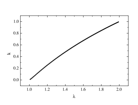
FIG. 8.: The exponent $k$ defined in Eq. (64) as a function of $\lambda$.

The form that the ratio of successive coefficients takes also gives us an idea of the number of coefficients we will need to approximate $d(y)$ for a given value of $y$. Assuming that a particular term in the series becomes significant when it is the same size as the previous term, we find that the maximum order that we need in our approximation goes like

$$l\sim y^{1/k}\ .$$ (65)

Thus for $\lambda$ near $2$, the number of terms needed will grow approximately linearly with $y$. On the other hand, for $\lambda$ near 1, where $k\rightarrow 0$, the number of terms will increase much more quickly with $y$.

B $h(\tilde{y})$

We now turn to the dual function, $h$. Above, we found the series in $d(y)$ for $\lambda\rightarrow 1$. From this, we can immediately write down $h(\tilde{y})$ when $\xi\rightarrow 1$. The series is identical in form, with $\lambda$ replaced by $\xi$, so that

$$h(\tilde{y})=\tilde{y}-\tilde{y}^{2}+\tilde{y}^{3}+\ldots\ ,$$ (66)

which converges for $0<\tilde{y}<1$ to $h(\tilde{y})=\tilde{y}/(1+\tilde{y})$. For the general case, we again examine the ratios of successive coefficients, $|s_{l}/s_{l+1}|$. We find the ratios flatten to constant values, for large enough $l$ , indicating finite radii of convergence. The radii get smaller and vanish as $\xi$ approaches zero as shown in Fig. 9.

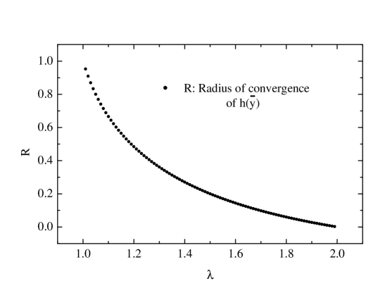
FIG. 9.: Radius of convergence of $h(\tilde{y})$ as a function of $\lambda$.

Note that for any value of $\xi$ tried, we found good evidence that $lim_{n\rightarrow\infty}\widehat{S}_{n}=-1.5$, indicating a $(\tilde{y}-\tilde{y}_{c})^{1/2}$ behavior. This is consistent with the existence of a quadratic minimum for the inverse function discussed below.

C $y(d)$)

We already found above that for $\lambda=2$, $y(d)=-\ln(1-d)$. This series converges for $0<d<1$, which is the required range. (Since $y$ must diverge as $d\rightarrow 1$, it is not surprising that our series breaks down at this point.) For $\lambda\rightarrow 1$, we have, inverting the $d$-function found above, that $y(d)=d/(1-d)$ which also converges for $0<d<1$. We find empirically from the analysis of ratios that for all $1<\lambda<2$, $y(d)$ converges in the region $0<d<1$.

The analysis of the extrapolated slope for various $\lambda$ gives convincing evidence that the main singularity has the form

$$y(d)\sim d^{-1/\gamma}\ .$$ (67)

This can be seen with short series when $\lambda$ is close to one and requires larger and larger series as $\lambda$ gets close to 2.

D $\tilde{y}(h)$)

The $\tilde{y}(h)$ series behaves similarly to the $y(d)$, having a radius of convergence of $1$ for all $\xi$. In this case, the ratio of coefficients $t_{l}/t_{l+1}$ approaches $1$ smoothly from below as $l$ increases, for larger $\xi$ Around $\xi=0.4$, small oscillations begin to appear in the curve. As $\xi$ becomes smaller, these oscillations grow and become quite large for $\xi$ smaller than $0.1$ (Fig. 10). However, in all cases studied, the ratio eventually approaches $1$, for large enough $l$.

FIG. 10.: Ratios of coefficients for $\tilde{y}(h_{n})$ with $\xi=0.1$.

A detailed study shows that if we continuate $\tilde{y}(h)$ for negative values of $h$ using the series expansion, the function develops a quadratic minimum when $h\rightarrow-1$. The absolute value of this minimum found in all examples studied is compatible with the radius of convergence of the inverse function and the square root singularity of the $h(\tilde{y})$ discussed above.

As one can guess by looking at Fig. 2, the analysis of the extrapolated slope is intricated. However, if we calculate enough terms and if $\lambda$ is not too close to 2, one can get approximate results which are consistent with a main singularity of the form

$$\tilde{y}(h)\sim h^{-\gamma}\ .$$ (68)

For instance, just by looking at the asymptotic behavior of Fig. 2, one can see that $\gamma\simeq 1.4677$, as expected, with errors of the order $10^{-4}$.

VI The susceptibility of the one-variable model

Now that we can calculate $h_{n}$ and $d_{n}$, we can construct the (infinite-volume limit) susceptibility. If we focus on the HT fixed point and the $h$-map, we get the HT expansion in terms of $h_{0}=\beta/\beta_{c}$. On the other hand, to understand the susceptibility’s behavior near to the fixed point, we need to expand in terms of $d_{0}=1-\beta/\beta_{c}$. Finally, we consider the possibility of combining the two expansions in the crossover region.

A The HT expansion of the susceptibility

We could find the HT expansion from the finite-volume susceptibility found in the previous section, by taking the large-$n$ limit. Since $0<\xi<1$, all of the $\xi^{n}$ terms will drop out. However, we can also construct the large-$n$ limit directly. Recalling that $\chi_{n}=(h_{n}/h_{0})\xi^{-n}$, and using $\tilde{y}_{n}=\xi^{n}\tilde{y}_{0}$, we find that

$$\chi_{n}=\frac{h_{n}\tilde{y}_{0}}{h_{0}\tilde{y}_{n}}=\frac{h(\tilde{y}_{n})\tilde{y}_{0}}{h_{0}\tilde{y}_{n}}\ .$$ (69)

The infinite-volume limit becomes:

$$\chi\equiv\lim_{n\rightarrow\infty}\chi_{n}=\frac{\tilde{y}_{0}}{h_{0}}\lim_{n\rightarrow\infty}\frac{h(\tilde{y}_{n})}{\tilde{y}_{n}}\ .$$ (70)

Using the $\tilde{y}$-expansion for $h$, we find

$$\frac{h(\tilde{y}_{n})}{\tilde{y}_{n}}=1-\frac{\tilde{y}_{n}}{\xi}+\ldots$$ (71)

As $n\rightarrow\infty$, $\tilde{y}_{n}\rightarrow 0$, so the infinite volume limit of the susceptibility is:

$$\chi=\frac{\tilde{y}_{0}}{h_{0}}=\frac{\tilde{y}(h_{0})}{h_{0}}\ .$$ (72)

Using the $h$-expansion for $\tilde{y}$, we get the HT expansion for the susceptibility:

$$\chi=1+\frac{1}{\xi}h_{0}+\frac{2}{\xi(1+\xi)}h_{0}^{2}+\ldots$$ (73)

Using $\chi_{n}=(h_{n}/h_{0})\xi^{-n}$, we find the HT expansion for the finite-volume susceptibility (recall that $h_{0}=\beta/\beta_{c}$):

$$\chi_{n}=1+\frac{1-\xi^{n}}{\xi}h_{0}+\ldots$$ (74)

We can find the error in the finite-volume susceptibility as an approximation to $\chi$. For large $n$ (small $\tilde{y}_{n}$), we get $\chi_{n}\simeq\chi(1-\tilde{y}_{n}/\xi)=\chi(1-\xi^{n-1}\tilde{y}_{0})$. The relative error is then:

$$\frac{\chi-\chi_{n}}{\chi}\simeq\xi^{n-1}\tilde{y}_{0}=\xi^{n-1}h_{0}\chi\ .$$ (75)

This behavior is observed [9] in the approach to infinite volume for the HM.

B Expansion near the critical point

In addition of using the HT expansion (expressing $\chi$ in terms of $h_{0}$), we would also like to have an expansion in terms of the dual variable $d_{0}$. Multiplying the numerator and the denominator of Eq. (72) by $y_{0}^{\gamma}$, we obtain

$$\chi=\frac{\Theta}{(1-d_{0})y(d_{0})^{\gamma}}\ .$$ (76)

with

$$\Theta\equiv\tilde{y}_{0}y_{0}^{\gamma}\ .$$ (77)

But since $\lambda^{\gamma}=\xi^{-1}$, we have also

$$\Theta=\tilde{y}_{n}y_{n}^{\gamma}\ ,$$ (78)

for any $n$. In other words, $\Theta$ is RG invariant. Due to the discrete nature of our RG transformation, $\Theta$ is not exactly a constant. If expressed in terms of ln($y_{0}$), $\Theta$ is a periodic function of period ln$\lambda$. However, for $\lambda$ not too close to 2, the non-zero Fourier modes are very small [14].

C Numerical evidence for overlapping domains of convergence

As we have seen above, $\tilde{y}_{n}y_{n}^{\gamma}$ is the same for every $n$. We can thus pick $n$ such that we are just in the crossover region and $both$ expansions have a reasonable chance to be accurate. In order to test the accuracy of the approximations $y_{app}(d)$ (series expansion up to a certain order) for various $n$, we have prepared an empirical sequences of $d_{n}$ starting with $d_{0}=10^{-8}$. We have then tested the scaling properties by calculating

$$D_{n}=|\left[y_{app}(d_{n})/(y_{0}\lambda^{n})\right]-1|\ ,$$ (79)

where $y_{0}$ was calculated with 16 digits of accuracy. Optimal approximations are those for which $D_{n}\simeq 10^{-16}$. For such approximation, scaling is as good as it can possibly be. Indeed, due to the peculiar way numerical errors propagate [22], one does not reach exactly the expected level $10^{-16}$ (more about this question in section IX). We can define a similar dual quantity by replacing $d$ by $h$ and $y$ by $\tilde{y}$. In this case, $\tilde{y}_{0}$ is estimated with the same accuracy as $y_{0}$ by stabilizing $\tilde{y}(h_{n})/\xi^{n}$, for large enough $n$.

We have performed this calculation for $\lambda=$ 1.1, 1.5 and 1.9. The conclusions in the three cases are identical. For $n$ large enough, the $D_{n}$ of $y$ starts increasing from $10^{-16}$ until it saturates around 1. By increasing the number of terms in the expansion, we can increase the value of $n$ for which we start losing accuracy. Similarly, for $n$ low enough, the $D_{n}$ of $\tilde{y}$ starts increasing etc… We want to know if it is possible to calculate enough terms in each expansion to get scaling with some desired accuracy for both functions. The answer to this question is affirmative according to Fig. 11 for $\lambda=1.5$.

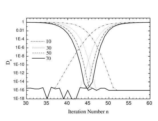
FIG. 11.: Departure from scaling $D_{n}$ defined in the text, for $y$ (curves reaching 1 to the right) and $\tilde{y}$ (curves reaching 1 to the left). In each cases, we have considered approximations of order 10 (dot-dashes), 30 (dots), 50 (dashes) and 70 (solid line). The value of $\lambda$ is 1.5.

One sees, for instance, that with 10 terms in each series, we have scaling with about 1 part in 1000 near $n=45$ for both expansions. The situation can be improved. For 70-70 expansions, an optimal accuracy is reached from $n=44$ to 46. For the other values of $\lambda$ quoted above, similar conclusions are reached, the only difference being the optimal values of $n$.

D Analysis of the RG invariant

Another evidence for overlapping convergence is that we can calculate the RG invariant $\Theta$ for a certain range of $y_{n}$. To evaluate $\Theta$, we use the series expansions for $\tilde{y}$ and $d$, cutting each off at some order:

$$\tilde{y}(1-d(y))\simeq\sum_{i=1}^{\tilde{m}}t_{i}(1-\sum_{j=1}^{m}s_{j}y^{j})^{i}\ ,$$ (80)

where $s_{l}$ and $t_{l}$ are the $l$th coefficients in the $d$ and $\tilde{y}$ series, respectively. The $d$ series is more accurate the smaller is the value of $y$, while the $\tilde{y}$ series is more accurate for $d(y)$ close to $1$, which means large values of $y$. Thus for $y$ very large, we need many terms in the $d$ series, while we need less terms in the $\tilde{y}$ series. On the other hand, when $y$ is very small, we need a large value for $\tilde{m}$ and a relatively small $m$. We have found that, given a fixed value of $m+\tilde{m}$, the most accurate values for $\Theta$ are obtained when $m\simeq\tilde{m}$. In Fig. 12, we show $\Theta$ calculated by keeping $50$ terms each in the expansions for $y$ and $\tilde{y}$. The result is plotted against $\ln(y)$. We used $\xi=0.1$, which makes the oscillations much larger than, for example, near to $\xi=2^{-2/3}$. Near the fixed points, we need more terms in the appropriate series to get accurate results.

FIG. 12.: The invariant function $\Theta$, calculated at $\xi=0.1$, and plotted against $\ln(y_{0})$.

We can study the oscillation we see in $\Theta$ by looking at its Fourier expansion. Since $\Theta$ is periodic in $\ln y_{0}$, we can express

$$\Theta(y_{0})=y_{0}^{\gamma}\tilde{y}(1-d(y_{0}))=\sum_{p}a_{p}e^{ip\omega\ln y_{0}}\ ,$$ (81)

where $\omega\equiv 2\pi/\ln\lambda$. The coefficients are given as

$$a_{p}=\frac{1}{\ln\lambda}\int_{y_{a}}^{\lambda y_{a}}y^{\gamma-1-ip\omega}\tilde{y}(1-d(y))dy\ ,$$ (82)

for some $y_{a}$ of our choice.

As an example, we calculate $a_{0}$ for $\xi=0.1$ where the oscillations are substantial. The choice of the interval can be infered from Fig. 12. If we had infinite series, the function would be exactly periodic. For finite series, we see that $y_{a}$ cannot be too large or too small. For intermediate values, we obtain $a_{0}\simeq 6.06676$. In Fig. 13, we show this constant term subtracted from the $\Theta$ we evaluated above. What remains is oscillations about $0$. We also calculated $a_{1}$ (using $y_{a}=\lambda$ so that we keep information about the phase constant as well as the amplitude). We construct the first oscillating mode from this, and in Fig. (14) we show the result of subtracting out this in addition to the constant term. We are left with even smaller oscillations, from the $a_{2}$ term.

FIG. 13.: Same as previous plot, with the constant term from the Fourier expansion subtracted out.

FIG. 14.: Same as previous plot, with first oscillating term from the Fourier expansion subtracted out.

In Fig. 14, one notices that when $\ln(y_{0})$ is of the order of 1.7, the breakdown of the approximation starts with small numerical noise before the complete breakdown near $\ln(y_{0})\simeq 2.2$ is observed (see Fig. 12).

VII SCALING VARIABLES IN THE HIERARCHICAL MODEL

In the one-variable model, we learned that we could express the basic mapping parameter, $h_{n}$, the distance from the HT fixed point, in terms of either of two new variables, $y_{n}$ or $\tilde{y}_{n}$. The first of these variables transforms multiplicatively with $\lambda$, the eigenvalue near the unstable fixed point, while the second transforms multiplicatively with $\xi$, the eigenvalue near the HT fixed point.

We would like to extend these methods to Dyson’s HM. We will express the parameters of the model in terms of two new sets of variables $y_{n,1},\ldots,y_{n,l_{max}}$ and $\tilde{y}_{n,1},\ldots,\tilde{y}_{n,l_{max}}$, where $l_{max}$ is equal to the number of parameters we keep in the mapping. These are the scaling variables.

Near to the unstable fixed point we find a set of eigenvectors and eigenvalues which control the RG flows in the linearized region. We use the notation $\lambda_{i}$ for the $i$th eigenvalue, ordered in size from greatest to least. For each of these eigenvalues, we introduce a variable $y_{n,i}$ which transforms under the RG transformation as $y_{n+1,i}=\lambda_{i}y_{n,i}$. We denote $\tilde{\lambda}_{i}$ for the eigenvalues in the linear HT region, similarly defining variables which transform as $\tilde{y}_{n+1,i}=\tilde{\lambda}_{i}\tilde{y}_{n,i}$. Then we can expand each of the parameters in terms of each set of scaling variables. Our first task will be to use special coordinates where the problem will be solved at the linear level. To use a relativistic analogy, the transformations leading to such a system of coordinates (the “linear scaling variables”), can be interpreted as a “translation” or shift and a “rotation” or more generally a linear transformation.

A Transformation properties under translation

We previously considered truncation in the $a_{n,l}$ parameters. Unfortunately, this approximation becomes less accurate if we are interested in the critical region. We would like to investigate a truncation that works near to the nontrivial fixed point. We re-express the basic recursion in terms of a new set of parameters, which give the distance from the nontrivial fixed point. For notational convenience, we first rewrite the unnormalized recursion given in Eq. (18), using the “structure constants”:

$$u_{n,\sigma}=\Gamma_{\sigma}^{\mu\nu}a_{n,\mu}a_{n,\nu}\ ,$$ (83)

with

$$\Gamma_{\sigma}^{\mu\nu}=\left\{\begin{array}[]{r@{\quad,\quad}l}(c/4)^{\mu+\nu}\ \frac{(-1/2)^{\mu+\nu-\sigma}(2(\mu+\nu))!}{(\mu+\nu-\sigma)!(2\sigma)!}&\ {\rm for}\ \mu+\nu\geq\sigma\\ 0&\ {\rm otherwise}\ .\end{array}\right.$$ (84)

These zeroes can be understood as a “selection rule” associated with the fact that $a_{n,l}$ is of order $\beta^{l}$ as explained in section II. If we follow the truncation procedure explained in section II, the indices simply run over a finite number of values. We use “relativistic” notations. Repeated indices mean summation. The greek indices indices $\mu$ and $\nu$ go from $0$ to $l_{max}$, while latin indices $i$, $j$ go from 1 to $l_{max}$. Obviously, $\Gamma_{\sigma}^{\mu\nu}$ is symmetric in $\mu$ and $\nu$. By construction, $a_{n,0}=1$ and we can write the normalized recursion in the form:

$$a_{n+1,l}=\frac{{\cal M}_{l}^{i}a_{n,i}+\Gamma_{l}^{ij}a_{n,i}a_{n,j}}{1+{\cal M}_{0}^{i}a_{n,i}+\Gamma_{0}^{ij}a_{n,i}a_{n,j}}\ ,$$ (85)

with

$${\cal M}_{\eta}^{i}=2\Gamma_{\eta}^{0i}\ .$$ (86)

Let assume that we know a fixed point of the recursion formula $a_{n,l}=a_{l}^{*}$. We then introduce intermediate variables $g_{n,l}$ which are zero at the fixed point:

$$a_{n,l}\equiv a_{l}^{*}+g_{n,l}\ .$$ (87)

Plugging this relation into Eq. (85), using the fixed point properties, subtracting the fixed point and reducing to the same denominator, we obtain a recursion formula for the $g_{n,l}$ having the same form as Eq. (85) with the substitutions

$$\Gamma_{\eta}^{ij}\rightarrow\frac{1}{u_{0}^{*}}(\Gamma_{\eta}^{ij}-(1-\delta_{\eta 0})a_{\eta}^{*}\Gamma_{0}^{ij})\ ,$$ (88)

and

$${\cal M}_{\eta}^{i}\rightarrow\frac{1}{u_{0}^{*}}({\cal M}_{\eta}^{i}+2\Gamma_{0}^{ij}a_{j}^{*}+(1-\delta_{\eta 0})({\cal M}_{0}^{i}+2\Gamma_{0}^{ij}a_{j}^{*})a_{\eta}^{*}\ ,$$ (89)

where $u_{0}^{*}\equiv\Gamma_{0}^{\mu\nu}a_{\mu}^{*}a_{\nu}^{*}$.

These equations express the transformation properties of the structure constants under a translation (shift) of the coordinates. In particular if $a_{l}^{*}=0$ (as for the HT fixed point), one can see that since $\Gamma_{00}^{0}=1$, the transformation reduces to the identity. We will now study the transformation properties under changes of coordinates which will diagonalize the linear RG transformation matrix ${\cal M}_{i}^{j}$.

B Diagonalization of the linear RG

The diagonalization of the linear ${\cal M}_{i}^{j}$ near the HT fixed point is quite simple because it is of the upper triangular form. The eigenvalues are just the diagonal terms. From Eq. (84), one sees that $l$th diagonal term is given as

$$\tilde{\lambda}_{(r)}=2(c/4)^{r}\ .$$ (90)

This spectrum was obtained in Ref. [23] with a different method. This means that an $l\times l$ truncated version of the matrix will have eigenvalues which are identical to the first $l$ eigenvalues of the full HM map. Furthermore, the $l$th eigenvector will contain only $l$ non-zero entries. This means that if we truncate to $a_{l_{max}}$, we are simultaneously truncating to the parameter space to a subspace spanned by the first $l_{max}$ eigenvectors. This “stability” is due to the special relationship existing between the HT expansion and the polynomial truncation explained in section II.

On the other hand, the linearized map near the nontrivial fixed point does not have these simple properties. The eigenvalues may be determined numerically from a truncated version of the linearized matrix. With a large enough truncation, we can find a certain number of the eigenvalues to any desired precision. We find that there is one eigenvalue larger than $1$, with all the rest less than $1$. Though we do not have a simple formula for these eigenvalues, we know that they do shrink in size quickly, similarly to the eigenvalues of the HT fixed point. For instance the numerical values for $c=2^{1/3}$ are $\lambda_{1}=1.42717\dots$, $\lambda_{2}=0.85941\dots$. A more complete list is given in Ref. [11].

Since ${\cal M}$ is not a symmetric matrix the left and right eigenvector are distinct.

$${\cal M}_{l}^{i}\psi^{r}_{i}=\lambda_{(r)}\psi^{r}_{l}$$ (91)

and

$$\phi_{r}^{l}{\cal M}_{l}^{i}=\lambda_{(r)}\phi_{r}^{i}\ .$$ (92)

The notation $(r)$ means that there is no sum on $r$. Since all the eigenvalues are distinct, one can normalize the eigenvectors in such a way that

$$\phi_{r}^{i}\psi^{r^{{}^{\prime}}}_{i}=\delta_{r}^{r^{{}^{\prime}}}\ .$$ (93)

Similarly a completeness relation (decomposition of the identity) can be obtained by summing over $r$:

$$\phi_{r}^{i}\psi^{r}_{j}=\delta_{j}^{i}\ .$$ (94)

In numerical calculations, the relations of orthogonality and completeness provide a reliable way to check the accuracy of the calculations.

We can thus diagonalize the linearized RG:

$$\phi_{r}^{l}{\cal M}_{l}^{i}\psi^{r^{{}^{\prime}}}_{i}=\lambda_{(r)}\delta_{r}^{r^{{}^{\prime}}}\ .$$ (95)

If we start with the transformation expressed in the general form Eq. (85) but with $a$ replaced by $g$ to indicate that the fixed point is at the origin, as in the previous subsection, we can define a new set of coordinates $d_{n,l}$, such that

$$g_{n,l}=\psi^{r}_{l}d_{n,r}\ ,$$ (96)

or, equivalently,

$$d_{n,r}=\phi_{r}^{l}g_{n,l}\ .$$ (97)

With these notations, all the structure constants transform according to the familiar rules of tensor analysis. Since $\phi$ and $\psi$ are inverse of each other, we can think of lower indices as covariant and upper indices as contravariant. As an example of transformation under Eq. (96), we have

$$\Gamma_{p}^{qr}\rightarrow\phi_{p}^{p^{{}^{\prime}}}\Gamma_{p^{{}^{\prime}}}^{q^{{}^{\prime}}r^{{}^{\prime}}}\psi^{q}_{q^{{}^{\prime}}}\psi^{r}_{r^{{}^{\prime}}}\ .$$ (98)

The other structure constants transform according to the same rules.

The eigenvectors are not determined uniquely even after normalizing. If $\psi^{r}_{i}$ and $\phi_{r}^{i}$ are components of normalized right and left eigenvectors, then $\psi^{r}_{i}=\alpha_{(r)}\psi^{r}_{i}$ and $\phi_{r}^{i}=\phi_{r}^{i}/\alpha_{(r)}$, where $\alpha_{(r)}$ is a constant, will work equally well. In the following, we will fix this ambiguity by requiring that the “other” fixed point be at $(1,1,\ldots)$ in the new coordinates.

C The Canonical Form

In summary, we can choose a system  of coordinate $d_{l}$ where the unstable fixed point will be at the origin of the coordinate and the HT fixed point at $(1,1,\dots)$, and such that the linear RG transformation is diagonal. In this system of coordinates, the RG transformation reads

$$d_{n+1,r}=\frac{\lambda_{(r)}d_{n,r}+\Delta_{r}^{pq}d_{n,p}d_{n,q}}{1+\Lambda^{p}d_{n,p}+\Delta_{0}^{pq}d_{n,p}d_{n,q}}\ ,$$ (99)

where the new structure constant are calculated from the original ones according to the transformation laws discussed in the previous two subsections.

Similarly, we can introduce new coordinates $h_{l}$, so that

$$a_{n,l}=\tilde{\psi}^{r}_{l}h_{n,r}\ ,$$ (100)

and take the eigenvectors so that the unstable fixed point is at $(1,1,\ldots)$ in the new system of coordinates. Note that the form of the eigenvectors guarantees that $h_{n,l}$ is of order $\beta^{l}$. This can be seen by inverting Eq. (100) using the matrix of left eigenvalues. Due to the upper-diagonal form, the second left eigenvector has its first entry equal to zero, the third its first two entries etc… . In this new system, the RG transformation reads

$$h_{n+1,r}=\frac{\tilde{\lambda}_{(r)}h_{n,r}+\tilde{\Delta}_{r}^{pq}h_{n,p}h_{n,q}}{1+\tilde{\Lambda}^{p}h_{n,p}+\tilde{\Delta}_{0}^{pq}h_{n,p}h_{n,q}}\ .$$ (101)

D Expansions in terms of the scaling variables

We would like to express the evolution of the canonical coordinates in terms of functions of the scaling variables:

$$d_{n,r}=\sum_{i_{1},i_{2},\ldots}s_{r,i_{1}i_{2}\ldots}y_{n,1}^{i_{1}}y_{n,2}^{i_{2}}\ldots\ ,$$ (102)

where the sums over the $i$’s run from $0$ to infinity in each variable and $y_{n,l}=\lambda_{(l)}^{n}y_{0,l}$. In practice, we expand in terms of some finite number of the scaling variables, less than or equal to the number of $d$ parameters we have truncated to. Using the notation ${\mathbf{i}}=(i_{1},i_{2}\ldots$) and the product symbol, we may rewrite the expansion as

$$d_{n,r}=\sum_{\mathbf{i}}s_{r,\mathbf{i}}\prod_{m}y_{n,m}^{i_{m}}$$ (103)

Using the transformation law for the scaling variables, we have

$$d_{n+1,r}=\sum_{\mathbf{i}}s_{r,\mathbf{i}}\prod_{m}(\lambda_{(m)}y_{m})^{i_{m}}\ .$$ (104)

Each constant term, $s_{r,0,0,\ldots}$, is zero, as the scaling variables vanish at the fixed point. From Eq. (99), we see that all but one of the linear terms are zero for each value of $r$. The remaining term is the one proportional to the $r$th scaling variable. We take these coefficients to be $1$, so that the $d_{n,r}\simeq y_{n,r}$ for small $y_{n,r}$. For the higher-order terms, we obtain the recursion

$$s_{r,\mathbf{i}}=\frac{\sum_{\mathbf{j}+\mathbf{k}=\mathbf{i}}(\Delta_{r}^{pq}s_{p,\mathbf{j}}s_{q,\mathbf{k}}-s_{r,\mathbf{j}}\prod_{m}\lambda_{(m)}^{j_{m}}\Lambda^{p}s_{p,\mathbf{k}})-\sum_{\mathbf{j}+\mathbf{k}+\mathbf{l}=\mathbf{i}}s_{r,\mathbf{j}}\prod_{m}\lambda_{(m)}^{j_{m}}\Delta_{0}^{pq}s_{p,\mathbf{k}}s_{q,\mathbf{l}}}{\left(\prod_{m}\lambda_{(m)}^{i_{m}}-\lambda_{r}\right)}\ .$$ (105)

The calculation can be organized in such way that the r. h. s. of the equations are already known. This will be the case for instance if we proceed order by order in $\sum_{q}i_{q}$, the degree of non-linearity. As one can see, this expansion may suffer from “small denominator problems”. This issue will be discussed elsewhere [24].

We can likewise expand each $h_{n,r}$ in terms of scaling variables $\tilde{y}_{n,1},\tilde{y}_{n,2},\ldots$. The derived recursions are identical in form to those derived above. From Eq. (90), one sees that the denominator will vanish for some equations and unless the numerator is also zero, the expansion is ill-defined. Again this question will be discussed elsewhere [24]. In the following, we will only use the expansion for the $d$-functions.

E Expansion of the scaling variables

One can likewise find expansions of the scaling variables in terms of the canonical coordinates, by setting

$$y_{n,r}=\sum_{\mathbf{i}}u_{r,\mathbf{i}}\prod_{m}d_{n,m}^{i_{m}}\ ,$$ (106)

and requiring that when ${\bf d}_{n}$ is replaced by ${\bf d}_{n+1}$, the function is multiplied by $\lambda_{(r)}$. Since ${\bf d}_{n+1}$ has a denominator, it needs to be expanded for instance in increasing order of non-linearity. The same considerations applies for $\tilde{y}$. Note that small denominators may also be present in these calculations. However, the calculation of $y_{1}$ and $\tilde{y}_{1}$ is free of such a problem since the largest eigenvalue cannot be written as product of lower eigenvalues smaller than 1.

It is in principle simple to obtain these expansions order by order in the degree of non-linearity, however there exists some practical limitations. For instance, if we want to calculate all the non-linear terms of order 10 in any of the variables, with $l_{max}$=30, we need to calculate and store $30^{10}\sim 10^{15}$ numbers. In the next section, we show that one can organize these calculations in a way which allows accurate answers for the susceptibility.

F The susceptibility

From Eqs. (6) and (100), we obtain

$$\chi_{n}=-(2/\beta)\tilde{\psi}^{r}_{1}h_{n,r}(2/c)^{n}\ .$$ (107)

For $n$ large enough, the linear behavior applies and the the $h_{n,r}$ get multiplied by $2(c/4)^{r}$ at each iteration. In the large $n$ limit, only the $r=1$ term survives and consequently,

$$\chi=-(2/\beta)\tilde{\psi}^{1}_{1}{\rm lim}_{n\rightarrow\infty}h_{n,1}(2/c)^{n}\ .$$ (108)

Using the same method as in the one-variable model, we can in the limit replace $h_{n,1}$ by $\tilde{y}_{n,1}$ and obtain

$$\chi=-(2/\beta)\tilde{\psi}^{1}_{1}\tilde{y}_{0,1}\ .$$ (109)

This allows us to write

$$\chi=-(2/\beta)\tilde{\psi}^{1}_{1}\Theta\tilde{y}_{0,1}^{-\gamma}\ ,$$ (110)

where $\gamma\equiv-\ln(\tilde{\lambda}_{1})/\ln(\lambda_{1})$ and $\Theta$ the RG invariant

$$\Theta\equiv\tilde{y}_{0,1}y_{0,1}^{\gamma}=\tilde{y}_{n,1}y_{n,1}^{\gamma}\ .$$ (111)

For reference, in the case $c=2^{1/3}$, $\tilde{\psi}^{1}_{1}\simeq-0.564$.

One can calculate the subtracted four-point function following the same procedure, namely expressing the $a_{n,l}$ in terms of the $h_{n,l}$. However, $\tilde{\lambda}_{1}^{2}>\tilde{\lambda}_{2}$ and one needs to go beyond the linear expansion to calculate these quantities.

VIII Approximations and numerical implementation

In this section, we show that it is possible to design approximations such that one can calculate the susceptibility using Eq. (111). For this purpose we have calculated an empirical series of $a_{n,l}$ with $c=2^{1/3}$, $\beta=\beta_{c}-10^{-8}$ and an initial Ising measure. Detail relevant for this calculations can be found in Refs. [9, 11, 22]. The calculations have been performed with $l_{max}=30$, a value for which at the $\beta$ considered, the errors due to the truncation are of the same order as those due to the numerical errors. These errors are small enough to allow a determination of the susceptibility with seven significant digits if we use double precision.

The empirical flow proceeds in two steps. First, the flow goes from the initial mesure to close to the unstable fixed point. Second, the flow goes from close to the unstable fixed point to the HT fixed point. The first step depends on the choice of the initial measure and will not be discussed in full detail. Our main goal will be to show that it is possible to construct nonlinear expansions which allow to describe accurately the second step. We now discuss the flow chronologically. In order to keep track of the chronological sequence, we postponed the technical discussion of the convergence of the series to section IX. In this section, the results are simply quoted.

Our choice of $\beta$ means that we start near the stable manifold. After about 25 iterations, we start approaching the unstable fixed point and the linear behavior $d_{n+1,l}\simeq\lambda_{l}d_{n}$ becomes a good approximation. During the next 20 iterations, the irrelevant variables die off at the linear rate and at the same time we move away from the fixed point along the unstable direction, also at the linear rate. At $n=47$ we are in good approximation on the unstable manifold and $d_{n,2}$ becomes proportional to $d_{n,1}^{2}$. In other words, the non-linear terms are taking over. At this point, we can approximate the $d_{n,l}$ as functions of $y_{1}$ only: $d_{n,l}\simeq d_{l}(\lambda_{1}^{n}y_{1},0,0,\dots)$. This approximation is consistent in the sense that if $y_{2}=0$ at $n=0$ then it is also the case for positive $n$.

We have calculated $d_{l}(y_{1},0,0,\dots)$ up to order 80 in $y_{1}$ using Eq. (105). We have then inverted $d_{1}$ to obtain $y_{1}$. Given the empirical $d_{n,1}$ we then calculated the approximate $y_{n,1}$ and then used the other functions $d_{l}(y_{1})$ (with $l\geq 2$) to “predict” $d_{n,l}$. Comparison with the actual numbers were good in a restricted range. For $n=49$, the relative errors were less than a percent. They kept decreasing to less than one part in 10,000 for $n=54$ and then increased again. It will be shown in section IX that this corresponds to the fact that when $y_{1}$ becomes too large (a value of 3.7 first exceeded at $n=57$), the series expansion of $d_{1}$ diverges, unlike the one-variable model for which $d(y)$ is analytical. It will also be shown later that the quality of the approximation between $n=45$ and $n=55$ can be improved by by treating $y_{2}$, $y_{3},\dots$ perturbatively.

Near $n=55$, the presence of the HT fixed point starts dominating the flow but we are still far away from the linear regime. To take into account the non-linear effects, we have calculated $\tilde{y}_{1}({\bf h})$ up to order 11 in $\beta$. The reason for this modest order is that this is a multi-variable expansion. Recalling the discussion about the HT expansion in section II, we can count the number of terms at each order in $\beta$. At order two, we have $h_{1}^{2}$ and $h_{2}$, but since the linear transformation is diagonalized, $h_{2}$ will only appear in $\tilde{y}_{2}({\bf h})$. At order three, we have $h_{1}^{3}$, $h_{2}h_{1}$ and not $h_{3}$. It is easy to see that at order $l$, one has $p(l)-1$ terms, where $p(l)$ is the number of partitions of $l$. It has been known from the work of Hardy and Ramanujan that

$$p(l)\sim\frac{{\rm exp}(\pi\sqrt{2l/3})}{4\sqrt{3}l}\ .$$ (112)

It seems thus difficult to get very high order in this expansion. In order to fix the ideas, there are 41 terms at order 11, 489 at order 20 and 13,848,649 at order 80.

As explained in section IX, the expansion up to order 11 has a sufficient accuracy to take over at $n=55$. It also provides optimal (given our use of double precision) results for $n\geq 60$. As $n$ increases beyond 60, one can see the effect of each order disappear one after the other. Finally, the linear behavior becomes optimal near $n=130$. This concludes our chronological discussion. The main point made was that there exists a region in the crossover where both expansions are valid. We now proceed to justify empirically the claims made above.

IX Large-order behavior for the HM

A $y_{1}(d_{1})$

The behavior of $y_{1}(d_{1})$ obtained by the procedure described above, has been studied following the same methods as for the one-variable model. In order to provide a comparison, we have calculated the same quantities for the one-variable model with $\lambda=1.2573$. In the following, we call this model the “simplified model” (SM). For this special value, the critical exponents $\gamma$ of the two models coincide with five significant digits. We have good evidence that both series have a radius of convergence 1 as indicated by the extrapolated ratio defined in Eq. (12) reaching 1 at an expected rate (Fig. 15).

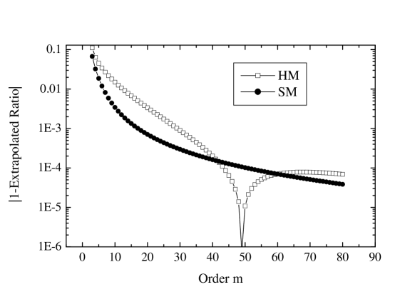
FIG. 15.: The absolute value of the difference between the extrapolated ratio and 1 for the HM (empty boxes) and the SM (full circles), as a function of the order.

Similarly, their extrapolated slopes seem to converge to the same value $1/\gamma-1\simeq-0.23026\dots$ as shown in Fig. 16.

FIG. 16.: The extrapolated slope $\hat{S}_{m}$ for the HM (empty boxes) and the SM (full circles) as a function of the order .

In conclusion, the function $y(d)$ for the SM is a reasonably good model to guess the asymptotic behavior of $y_{1}(d_{1})$.

B $d_{1}(y_{1})$

The situation is different for the inverse function $d_{1}(y_{1})$. A first look at the differences is given in Fig. 17.

FIG. 17.: Logarithm of the absolute value of the coefficients of the expansion of $d_{1}(y_{1})$ divided by the order, for the HM (empty boxes) and the SM (circles).

The quantity plotted in this figure will be used to discriminate between a finite and an infinite radius of convergence. If $|b_{m}|\sim R^{-m}$ as for a radius of convergence $R$, then we have ${\rm ln}(|b_{m}|)/m\sim-{\rm ln}(R)+A/m$ for some constant $A$. On the other hand, if $|b_{m}|\sim(m!)^{-\alpha}$ as for an infinite radius of convergence, then we have ${\rm ln}(|b_{m}|)/m\sim-\alpha({\rm ln}(m)-m)$. In the following, we will compare fits of the form $A_{1}+A_{2}/m$ and $B_{1}{\rm ln}(m)+B_{2}$.

We first consider the case of SM, where according to the our study in section V, we should have an infinite radius of convergence. This possibility is highly favored as shown in Fig. 18.

FIG. 18.: Comparison of fits of the form $A_{1}+A_{2}/m$ (dots)and $B_{1}{\rm ln}(m)+B_{2}$ (solid line) with the data provided in Fig. 17 for the SM (circles).

One sees clearly that the solid line is a much better fit. The chi-square for the solid line fit is 200 times smaller. In addition $B_{1}\simeq-B_{2}$ as expected. In conclusion, this analysis comfirms the ratio analysis done previously and favors strongly the inifite radius of convergence possibility.

The analysis for the HM is more delicate. One observes periodic “dips” in Fig. 17 which make the ratio analysis almost impossible. We have thus only considered, the “upper envelope” by removing the dips from Fig. 17. The fit represents an upper bound rather than the actual coefficients. The fits of the upper envelope are shown in Fig. 19

FIG. 19.: Comparison of fits of the form $A_{1}+A_{2}/m$ (solid line)and $B_{1}{\rm ln}(m)+B_{2}$ (dots) with selected points of the data in Fig. 17 for the HM (boxes).

The possibility of a finite radius of convergence is slightly favored, the chi-square being 0.4 of the one for the other possibility. Also, the second fit does not have the $B_{1}\simeq-B_{2}$ property. From $A_{1}\simeq-1.32$, we estimate that the radius of convergence is about 3.7.

C $\tilde{y}_{1}({\bf h})$

As explained in section VIII, one can calculate $\tilde{y}_{1}({\bf h})$ using an expansion in $\beta$. As in section V, we will use an empirical series $a_{n,l}$, calculate the corresponding $h_{n,l}$ an plug them in the scaling variables. This empirical series was calculated with an initial Ising measure and $\beta=\beta_{c}-10^{-8}$ (see Ref. [11]). Again we define a quantity $D_{n}$ as in Eq. (79) which is very small when we have good scaling and increases when the approximation breaks down. The results are shown in Fig. 20 for successive orders in $\beta$.

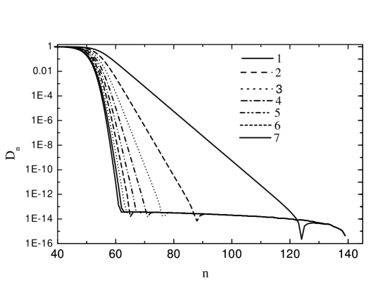
FIG. 20.: The quantity $D_{n}$ defined in Eq. (79) for expansions of $\tilde{y}_{1}$ in $\beta$, at order 1 (solid line), 2 (dashes), 3 (dots), etc… for each iteration $n$.

The solid line on the right is the linear approximation. It becomes optimal near $n=130$. The next line (dashes) is the second order in $\beta$ expansion. It becomes optimal near $n=90$. Each next order gets closer and closer to be optimal near $n=60$. The last curve on the left is the order 9 approximation. It is hard to resolve the next two approximations on this graph.

The asymptotic value is stabilized with 16 digits and one may wonder why we get only scaling with 14 or 15 digits in Fig. 20. The reason is that we use empirical data and that numerical errors can add coherently as explained in Ref. [22]. This can be seen directly by considering the difference between two successive values of $D_{n}$ as shown in Fig. 21.

FIG. 21.: Difference between two successive $D_{n}$ in $10^{-16}$ units.

One sees that the numerical errors at each step tend to be negative more often than positive, and consequently there is a small “drift” which affects the last digits.

D overlapping domains of convergence

We can now look at the $D_{n}$ defined as in Eq. (79) for $y_{1}$ and $\tilde{y}_{1}$ together in Fig. 22.

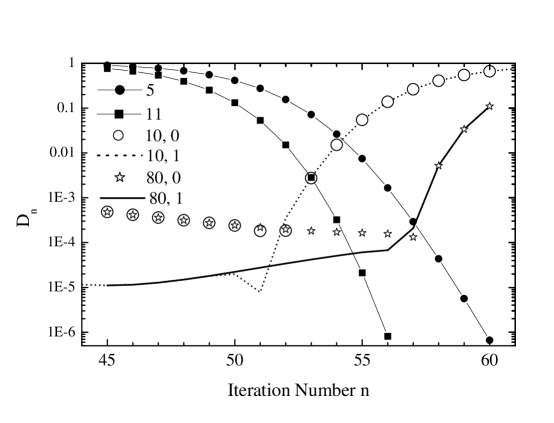
FIG. 22.: Values of $D_{n}$ for $\tilde{y}_{1}$ up to order 5 (filled circle) and 11 (filled boxes), and for $y_{1}$ up to order 10 in $d_{1}$ (empty circles) and with first order corrections in $y_{2}$ (dots), and up to order 80 in $d_{1}$ (empty stars) and with first order corrections in $y_{2}$ (solid line).

If we use an expansion of order 5 in $\beta$ for $\tilde{y}$ and of order 10 in $d_{1}$ for $y_{1}$, we can get scaling within a few percent for both variables at $n=54$. We can go below 1 part in 1000, with an expansion of order 11 in $\beta$ and order 80 in $d_{1}$. At this point, the main problem is that the effects of the subleading correction makes the scaling properties worse when $n\leq 57$ and $n$ decreases. One can improve the scaling properties by taking the effects of $y_{2}$ into account. A detailed study shows that one can estimate the subleading effects between $n=40$ and $n=45$. One finds that

$$\frac{y_{1}(d_{n,1})}{\lambda_{1}^{n}}\simeq 7.2778\times 10^{-9}-4.5\times 10^{-10}\times\lambda_{2}^{n}$$ (113)

It is thus possible to get a function scaling better by subtracting these correction. This improve the scaling properties by almost one order of magnitude near $n=54$ and by almost two order of magnitude near $n=45$. It is likely that our approximation of having a single scaling variable can be corrected order by order in $y_{2}$, $y_{3}$ etc… .

X conclusions

We have shown in two examples that the susceptibility can be expressed in terms of the scaling variables corresponding to the two fixed points governing the HT flows. We have given convincing evidence that the expansions of these variables have overlapping domains of convergence. Several interesting questions remain to be discussed.

We have not discussed in detail the initial approach of the unstable fixed point. We have just shown that it can in principle be incorporated by calculating the subleading corrections in $y_{2}$, $y_{3}$ etc… This study depends on the details of the initial measure. A particularly interesting set of initial measures are the Landau-Ginzburg models in the vicinity of the Gaussian fixed point. We can use the usual perturbation theory in the quartic (or higher orders) coupling constant to construct the scaling variables associated with the Gaussian fixed point following the procedure described above, and interpolate between the Gaussian fixed point and the unstable fixed point.

The question of small denominators and resonances have been circumvented by using only quantities which are free of this problem (namely $y_{1}$ and $\tilde{y}_{1}$ ) in our calculation of the susceptibility. The effects of the small denominators of the other scaling variables is a complex topic presently under study [24].

We emphasize that the complete knowledge of the scaling functions and their inverse provides analytical expressions for all the thermodynamic quantities at any volume (see Eq. (57) in the simplified model). In practical calculations, one is naturally led to combine different expansions and it is thus important to use sets of interactions which are compatible, as done in Ref. [3] for gauge theories.

- [1] K. Wilson, Phys. Rev. D 3, 1818 (1971).
- [2] K. Wilson and J. Kogut, Phys. Rep. 12, 75 (1974).
- [3] P. de Forcrand et al., Nucl. Phys. B 577, 263 (2000).
- [4] A. Gonzalez-Arroyo and M. Okawa, Phys. Rev. D 35, 672 (1987).
- [5] F. Dyson, Comm. Math. Phys. 12, 91 (1969).
- [6] G. Baker, Phys. Rev. B 5, 2622 (1972).
- [7] G. Baker and G. Golner, Phys. Rev. B 16, 2080 (1977).
- [8] D. Kim and C. Thomson, J. Phys. A 10, 1579 (1977).
- [9] J. Godina, Y. Meurice, M. Oktay, and S. Niermann, Phys. Rev. D 57, 6326 (1998).
- [10] J. Godina, Y. Meurice, and M. Oktay, Phys. Rev. D 57, R6581 (1998).
- [11] J. Godina, Y. Meurice, and M. Oktay, Phys. Rev. D 59, 096002 (1999).
- [12] F. Wegner, Phys. Rev. B 3, 4529 (1972).
- [13] J. Cardy, Scaling and Renormalization in Statistical Physics (Cambridge University Press, Cambridge, 1996).
- [14] Y. Meurice and S. Niermann, Phys. Rev. E 60, 2612 (1999).
- [15] J. J. Godina, Y. Meurice, and M. Oktay, Phys. Rev. D 61, 114509 (2000).
- [16] H. Koch and P. Wittwer, Math. Phys. Electr. Jour. 1, Paper 6 (1995).
- [17] B. Nickel, in Phase Transitions, Cargese 1980, edited by M. Levy, J. L. Guillou, and J. Zinn-Justin (Plenum Press, New York, 1982).
- [18] Y. Meurice, G. Ordaz, and V. G. J. Rodgers, Phys. Rev. Lett. 75, 4555 (1995).
- [19] Y. Meurice, S. Niermann, and G. Ordaz, J. Stat. Phys. 87, 363 (1997).
- [20] P. Collet and J.-P. Eckmann, Iterated of the interval as dynamical systems (Birkhauser, Boston, 1980).
- [21] V. Arnold, Geometrical Methods in the Theory of Ordinary Differential Equations (Springer-Verlag, New York, 1988).
- [22] Y. Meurice and B. Oktay, Non-Gaussian numerical errors versus mass hierarchy, hep-lat/0005011.
- [23] P. Collet and J.-P. Eckmann, A Renormalization Group Analysis of the Hierarchical Model in Statistical Mechanics, Edited by J. Ehlers et al., Lecture Notes in Physics 74, (Springer-Verlag, Berlin, 1978).
- [24] Y. Meurice, in preparation.