GUTPA/00/06/02
Casimir scaling of SU(3) static potentials

Abstract

Potentials between static colour sources in eight different representations are computed in four dimensional $SU(3)$ gauge theory. The simulations have been performed with the Wilson action on anisotropic lattices where the renormalised anisotropies have been determined non-perturbatively. After an extrapolation to the continuum limit we are able to exclude any violations of the Casimir scaling hypothesis that exceed 5 % for source separations of up to 1 fm.

I Introduction

Non-perturbative QCD effects in general and the nature of the confinement mechanism in particular are theoretically challenging. At the same time these aspects are important for high energy and low energy particle and nuclear phenomenology. Several models of non-perturbative QCD have been proposed whose predictions happen to differ from each other substantially in some cases. Prominent examples are bag models [1, 2, 3, 4, 5], strong coupling and flux tube models [6, 7, 8, 9], bosonic string models [10, 11], the stochastic vacuum model [12, 13, 14], dual QCD [15, 16, 17], the Abelian Higgs model [18, 19], and instanton based models [20, 21, 22]. Lattice simulations of interactions between static colour sources offer an ideal environment for discriminating between different models of low energy QCD and to learn more about the confinement mechanism. They are easily accessible analytically and at the same time very accurate Monte Carlo predictions can be obtained [23, 24].

Despite the availability of a wealth of information on fundamental potentials, only few lattice investigations of forces between sources in higher representations of $SU(N)$ gauge groups exist. Most of these studies have been performed in $SU(2)$ gauge theory in three [25, 26, 27, 28] and four [29, 30, 31, 32, 33, 34, 35, 36] space-time dimensions. Zero temperature results for four dimensional $SU(3)$ can be found in Refs. [37, 38, 39, 40, 41, 42] while determinations of Polyakov line correlators in non-fundamental representation have been performed at finite temperature by Bernard [29, 30] for $SU(2)$ and in Refs. [43, 44, 45, 46] for $SU(3)$ gauge theory.

In our study we shall see that the so-called Casimir scaling hypothesis [25] is rather accurately represented by the lattice data while models predicting a different behaviour are definitely ruled out. Casimir scaling means that potentials between sources in different representations are proportional to each other with their ratios given by the respective ratios of the eigenvalues of the corresponding quadratic Casimir operators, which is exact in the case of two dimensional Yang-Mills theories. Our result is of particular interest with respect to recent discussions of the confinement scenario [47, 48, 49, 50, 51].

At distances $r>r_{c}\approx 1.2$ fm [39] non-fundamental sources will be screened and “string breaking” effects will be encountered that are incompatible with Casimir scaling. In the present study we restrict ourselves to distances smaller than the string breaking scale $r_{c}$.

This article is organised as follows: in Sec. II the lattice methods that we apply and our notations are introduced. A determination of the renormalised anisotropies and lattice spacings is presented in Sec. III. The potentials are then determined in Sec. IV before we conclude with a brief discussion.

II Notations and Methods

We denote the energy of colour sources, separated by a distance $r$, in a representation $D={\mathbf{3}},{\mathbf{6}},{\mathbf{8}},{\mathbf{1}}{\mathbf{0}},\ldots$ of the $SU(3)$ gauge group by $V_{D}(r,\mu)$, where $\mu$ denotes some cut-off scale on the gluon momenta, for instance an inverse lattice spacing, $\mu=\pi/a$. We shall also use the subscript “$F$” to label the fundamental (${\mathbf{3}}$) representation (or we may just omit the subscript in this case).

TABLE I.: Group theoretical factors for $SU(3)$. $D$ is the dimension of the representation, $(p,q)$ are the weight factors, $z=\exp(2\pi i/3)$, and $d_{D}=C_{D}/C_{F}$ denote ratios of quadratic Casimir charges.

$D$	$(p,q)$	$z^{p-q}$	$p+q$	$d_{D}$
3	$(1,0)$	$z$	1	1
8	$(1,1)$	1	2	2.25
6	$(2,0)$	$z^{*}$	2	2.5
$15a$	$(2,1)$	$z$	3	4
10	$(3,0)$	1	3	4.5
27	$(2,2)$	1	4	6
24	$(3,1)$	$z^{*}$	4	6.25
$15s$	$(4,0)$	$z$	4	7

The static potential,

$$V_{D}(r,\mu)=V_{D}(r)+V_{D,\mbox{self}}(\mu),$$ (1)

can be factorised into an interaction part, $V_{D}(r)$, and a self energy contribution, $V_{D,\mbox{self}}(\mu)$ that will diverge like $\mu/\ln\mu$ as $\mu\rightarrow\infty$ while $V_{D}(r)$ will assume universal values.

A (dimensionless) lattice potential $\hat{V}_{D}({\mathbf{R}},a)$ will resemble the corresponding continuum potential up to lattice artefacts,

$$V_{D}(Ra) = a^{-1}\left[\hat{V}_{D}({\mathbf{R}},a)-\hat{V}_{D,\mbox{self}}(a)\right]$$ (2)

$$\times \left[1+f_{D}(Ra,\hat{\mathbf{R}})a^{\nu}\right],$$ (3)

where $\nu$ is a positive integer number that will in general depend on the lattice action employed. We are concerned with Wilson-type gluonic actions [52]. In this case, $\nu=2$. Note that the coefficient function $f$ only depends on the combination $r=Ra$ and on the direction of ${\mathbf{R}}$ but not on $R$ itself. This guarantees that lattice artefacts are reduced as $r\gg a$ is increased.

The static potentials are obtained from fits to smeared [53, 23, 54] Wilson loops for $T\geq T_{\min}$ where $T_{\min}$ depends on ${\mathbf{R}}$, the statistical errors of the Wilson loops and the smearing algorithm employed. We define a Wilson loop in representation $D$,

$$W_{D}({\mathbf{R}},T)=\mbox{Tr}\,\left(\prod_{(n,\mu)\in\delta C({\mathbf{R}},T)}U_{D,n,\mu}\right),$$ (4)

where $\delta C({\mathbf{R}},T)$ denotes the oriented boundary of a (generalised) rectangle with spatial extent ${\mathbf{R}}$ and a temporal separation of $T$ lattice spacings. $(n,\mu)$ denotes an oriented link connecting the site $n$ with $n+\hat{\mu}$, $n$ is an integer four-vector that labels a lattice site and $\hat{\mu}$ is a unit vector pointing into a direction, $\mu\in\{1,2,3,4\}$. “Tr ” is the normalised trace, $\mbox{Tr}_{D}{\mathbf{1}}_{D}=\frac{1}{N_{D}}\mbox{tr}\,{\mathbf{1}}_{D}=1$, $N_{D}$ is the dimension of the representation $D$ and,

$$U_{D,n,\mu}={\mathcal{P}}\left\{\exp\left[i\int_{an}^{a(n+\hat{\mu})}\!dx_{\mu}\,A^{a}_{\mu}(x)T_{a}^{D}\right]\right\},$$ (5)

denotes a link variable in representation $D$, where $T_{a}^{D}$ is a generator of the gauge group. Our conventions are $[T_{a}^{D},T_{b}^{D}]=if_{abc}T_{c}^{D}$, where $f_{abc}$ are totally antisymmetric real structure constants. The normalisation is such that $\mbox{tr}\,T_{a}^{F}T_{b}^{F}=\delta_{ab}/2$. Now:

$$\langle W_{D}({\mathbf{R}},T)\rangle=c_{D}({\mathbf{R}},a)\exp\left[-\hat{V}_{D}({\mathbf{R}},a)T\right]\quad(T\rightarrow\infty).$$ (6)

The use of smeared Wilson loops turns out to be more suitable for numerical simulations than implementing the definition of Eq. (4); the spatial pieces of the Wilson loop are replaced by linear combinations of various paths that models the ground state wave function. As a result the overlap of the creation operator with this ground state, $c_{D}$, is enhanced and the $T\rightarrow\infty$ limit can effectively be realised at moderate $T$ values.

In numerical simulations one observes that the statistical error $\Delta W(T)$ of the expectation value of a smeared Wilson loop $\langle W(T)\rangle$ only weakly varies with $T$ [54]. From Eqs. (1) and (6) we therefore obtain the relation,

$$\frac{\Delta W(T)}{\langle W(T)\rangle}\propto\exp[\hat{V}(a)T]\propto\exp\left[\hat{V}_{\mbox{self}}(a)T\right]\quad(T\rightarrow\infty),$$ (7)

for the relative errors (which are directly proportional to the statistical uncertainty of the potential values). In tree level perturbation theory one finds,

$$\hat{V}_{D,\mbox{self}}(a)=c\,C_{D}\,g^{2}(a),\quad c=0.252731\ldots;$$ (8)

the self energy is proportional to the eigenvalue of the quadratic Casimir operator $C_{D}=\mbox{Tr}_{D}T_{a}^{D}T_{a}^{D}$ of the representation. This means that statistical errors will increase significantly as we investigate higher representations of the sources with bigger Casimir charges.

This self energy related problem motivates us to introduce an anisotropy parameter $\xi=a_{\sigma}/a_{\tau}\approx 4$ between spatial lattice resolution $a_{\sigma}$ and temporal lattice constant $a_{\tau}$. This results in a reduction of the self energy, $\hat{V}_{D,\mbox{self}}=c\,C_{D}\,\xi^{-1}g^{2}$, and therefore of the relative errors of smeared Wilson loops. However, at the end of the day we wish to measure distance and potential in the same units $a_{\sigma}$. This means that we do not gain anything from the factor $\xi$ within the above expression. Nevertheless, a $\xi>1$ still results in a reduced effective $g^{2}$ at fixed $a_{\sigma}$. Of course, equally well we could just have increased the size of our statistical ensemble by a factor four and worked at $\xi=1$.

Our main motivation for introducing an anisotropy is the possibility of reducing lattice artefacts. These are most prominent at small and at large distances: as long as $r$ is not much larger than $a_{\sigma}$ the cubic lattice structure is clearly visible. In lowest order perturbation theory these violations of rotational symmetry only depend on ${\mathbf{R}}$ and $a_{\sigma}$ while the order $g^{4}$ coefficients exhibit a weak dependence on $\xi$ too [55]. While we cannot hope to significantly reduce these small distance effects without decreasing $a_{\sigma}$, it is clear that on a lattice with temporal resolution $a_{\tau}$ one cannot reliably resolve masses $m\gg a_{\tau}^{-1}$. However, at $r\gg a_{\sigma}$ and in particular for representations $D$ with large Casimir charges situations, $V_{D}(r)a_{\sigma}\gg 1$, are easily encountered, unless $\xi\gg 1$.

Introducing an anisotropy also means that within any physical $t$ window we have more data points at our disposal. While this might help to gain more confidence in identifying effective mass plateaus we find that the additional data points are highly correlated and add little extra information, at least when one is only interested in the mass of the ground state within a given channel.

Our action reads,

$$S=-\beta\sum_{n}\left[\frac{1}{\xi_{0}}\sum_{i>j}\mbox{Tr}\,U_{n,ij}+\xi_{0}\sum_{i}\mbox{Tr}\,U_{n,i4}\right],$$ (9)

where $\beta=2N/[g^{2}(a_{\sigma},\xi)]$ is defined through the lattice coupling $g^{2}$ and $i,j\in\{1,2,3\}$. $U_{n,\mu\nu}=U_{n,\mu}U_{n+\hat{\mu},\nu}U^{\dagger}_{n+\hat{\nu},\mu}U^{\dagger}_{n,\nu}$ denotes the product of four link variables around an elementary square, the plaquette. With the above anisotropic Wilson action, the leading order lattice artefacts are proportional to $a_{\sigma}^{2}$ and $a_{\tau}a_{\sigma}=a_{\sigma}^{2}\xi^{-1}$. This means that along a trajectory of constant $\xi$ the continuum limit will be approached quadratically in $a_{\sigma}$. The relationship between the bare anisotropy $\xi_{0}$ appearing in the action Eq. (9) and the renormalised anisotropy $\xi$ is known in one loop perturbation theory [56]: $\xi=\xi_{0}[1+c_{1}(\xi_{0})g^{2}+\cdots]$. In Sec. III we will discuss our non-perturbative evaluation of $\xi$. Of course the function $\xi(g^{2},\xi_{0})$ is not unique and different non-perturbative definitions might differ from each other by terms of order $a_{\sigma}$.

Perturbation theory yields the relation between potentials in different representations $D$,

$$V_{D}(r,\mu)=d_{D}V_{F}(r,\mu),$$ (10)

where $d_{D}=C_{D}/C_{F}$. Table I contains all representations $D$, the corresponding weights $(p,q)$ and the ratios of Casimir factors, $d_{D}$, for $p+q\leq 4$. In $SU(3)$ we have $C_{F}=4/3$, and $z=\exp(2\pi i/3)$ denotes a third root of 1. Eq. (10) is known to hold to (at least) one loop (order $g^{4}$) perturbation theory at finite lattice spacing [57] and two loops (order $g^{6}$) in the continuum limit [58] of four dimensional Yang-Mills theories. The main purpose of this article is to investigate non-perturbatively to what extent the “Casimir scaling” relation Eq. (10) is violated.

In what follows $U$ denotes a group element in the fundamental representation of $SU(3)$, for instance the product of link variables around a closed contour. The traces of $U_{D}$ in various representations, $V_{D}=\mbox{tr}\,U_{D}$, can easily be expressed in terms of traces of powers of $U$,

$$V_{3} = \mbox{tr}\,U,$$ (11)

$$V_{8} = \left(|V_{3}|^{2}-1\right),$$ (12)

$$V_{6} = \frac{1}{2}\left[(\mbox{tr}\,U)^{2}+\mbox{tr}\,U^{2}\right],$$ (13)

$$V_{15a} = \mbox{tr}\,U^{*}\,V_{6}-\mbox{tr}\,U,$$ (14)

$$V_{10} = \frac{1}{6}\left[(\mbox{tr}\,U)^{3}+3\,\mbox{tr}\,U\,\mbox{tr}\,U^{2}+2\,\mbox{tr}\,U^{3}\right],$$ (15)

$$V_{24} = \mbox{tr}\,U^{*}\,V_{10}-V_{6},$$ (16)

$$V_{27} = |V_{6}|^{2}-|V_{3}|^{2},$$ (17)

$$V_{15s} = \frac{1}{24}\left[(\mbox{tr}\,U)^{4}+6(\mbox{tr}\,U)^{2}\mbox{tr}\,U^{2}+3(\mbox{tr}\,U^{2})^{2}\right.$$ (18)

$$+ \left.8\,\mbox{tr}\,U\,\mbox{tr}\,U^{3}+6\,\mbox{tr}\,U^{4}\right].$$ (19)

Note that $\mbox{Tr}_{D}U_{D}=\frac{1}{N_{D}}\mbox{tr}\,U_{D}=V_{D}/N_{D}$. Hence, the normalisation of $V_{D}$ differs by a factor $N_{D}$ from that of the Wilson loop $W_{D}$ of Eq. (4). Under the replacement, $U\rightarrow z\,U$, $W_{D}$ transforms like, $W_{D}\rightarrow z^{p-q}W_{D}$. Representations with $z^{p-q}=1$ have zero triality.

III Determining anisotropy and lattice spacing

We simulate $SU(3)$ gauge theory at the parameter values $(\beta,\xi_{0})=(5.8,3.10),(6.0,3.20)$ and $(6.2,3.25)$. From exploratory simulations with limited statistics and the published data of Refs. [59, 60, 61] we expect to find renormalised anisotropies $\xi\approx 4$ at these combinations. At the above parameter values volumes of $L_{\sigma}^{3}\times L_{\tau}=8^{3}\times 48$, $12^{3}\times 72$ and $16^{3}\times 96$ lattice sites have been realised, respectively. These volumes were chosen to keep the lattice extent about constant in physical units. In addition a volume of $12^{3}\times 48$ lattice sites has been simulated at $\beta=5.8$ to investigate possible finite size effects.

The gauge configurations have been obtained by randomly mixing Cabibbo-Marinari style [62] Fabricius-Haan heatbath [63] and Creutz overrelaxation [64] sweeps, where we cycled over the three diagonal $SU(2)$ subgroups. The probability of a heatbath sweep was set to be $1/5$. During each sweep the sites were visited subsequently for each of the four space-time directions of the links in sequential order. Measurements were taken after 2000 initial heatbath sweeps and the gauge configurations are separated from each other by 200 sweeps. In doing so, we did not find any signs of autocorrelation or thermalization effects for any of the investigated observables at any of the simulated parameter sets. In the case of $\beta=6.0$ one set of configurations was generated on a Sparc station after a cold start while another set of configurations was generated on a Cray J90, starting from a hot, random configuration. No statistically significant deviations between these two data sets were found either. We display our simulation parameters in Table II. $n_{\mbox{conf}}$ denotes the number of statistically independent configurations analysed in each case while $r_{0}\approx 0.5$ fm is the Sommer scale parameter [65], implicitly defined through the static potential,

$$\left.\frac{dV(r)}{dr}\right|_{r=r_{0}}=1.65.$$ (20)

TABLE II.: Simulation parameters, lattice spacings and linear lattice extents.

$\beta$	$L_{\sigma}$	$n_{\mbox{conf}}$	$r_{0}/a_{\sigma}$	$r_{0}/a_{\tau}$	$L_{\sigma}a_{\sigma}/r_{0}$
5.8	8	633	3.074(29)	12.45(11)	2.60(3)
5.8	12	139	3.052(34)	12.52(13)	3.93(4)
6.0	12	159	4.437(71)	18.12(24)	2.70(5)
6.2	16	133	6.106(66)	24.16(23)	2.62(3)

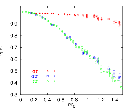
FIG. 1.: Ground state overlaps for the case of the fundamental potential determined from Wilson loops in three different orientations at $\beta=6.2$, $\xi_{0}=3.25$.

We label quantities associated with the fine grained direction by an index $\tau$ while $\sigma$ refers to coarse grained directions. On an anisotropic lattice various ways of associating the sides of smeared Wilson loops with these directions exist: $W_{\tau\sigma}(r/a_{\tau},t/a_{\sigma})$, $W_{\sigma\sigma}({\mathbf{r}}/a_{\sigma},t/a_{\sigma})$ and $W_{\sigma\tau}({\mathbf{r}}/a_{\sigma},t/a_{\tau})$. In the case of $W_{\tau\sigma}$ as well as for $W_{\sigma\sigma}$ the time coordinate points into a $\sigma$ direction. The spatial coordinate is identified with the $\tau$ direction in the first case and a $\sigma$ direction in the latter case. While the spatial connections within $W_{\tau\sigma}$ are parallel to the $\tau$ axis, in the case of $W_{\sigma\sigma}$ we realise planar off-axis configurations ${\mathbf{R}}\parallel(1,1,0)$ and ${\mathbf{R}}\parallel(2,1,0)$, in addition to on-axis separations. Finally, within $W_{\sigma\tau}$ the time coordinate is taken along the fine grained dimension and the spatial coordinate coarse grained. We determine $W_{\sigma\tau}$ for the standard separations [23], ${\mathbf{R}}\parallel(1,0,0),$ $(1,1,0),$ $(2,1,0),$ $(1,1,1),$ $(2,1,1),$ $(2,2,1)$.

In the spatially isotropic situation ($W_{\sigma\tau}$) we iteratively construct fat links in the standard way by replacing a given link by the sum of itself and the neighbouring four spatial staples with some weight parameter, $\alpha\geq 1$,

$$U_{n,i} \rightarrow P_{SU(3)}\left(\alpha\,U_{n,i}+\sum_{j\neq i}F_{n,j}\right),$$ (21)

$$F_{n,j} = U_{n,j}U_{n+\hat{\jmath},i}U^{\dagger}_{n+\hat{\imath},j}+U_{n-\hat{\imath},i}^{\dagger}U_{n-\hat{\imath},i}U_{n-\hat{\imath}+\hat{\jmath},j}.$$ (22)

$P_{SU(3)}$ denotes a projection operator, back onto the $SU(3)$ manifold. We employ the definition [23], $U=P_{SU(3)}(A)\in SU(3)$, $\mbox{Re}\,\mbox{Tr}\,UA^{\dagger}=\max$ and iterate Eq. (21) 26 times with $\alpha=2.3$.

We use a somewhat different novel smearing algorithm in the case of $W_{\tau\sigma}$ and $W_{\sigma\sigma}$ where the spatial volume is anisotropic with one fine and two coarse directions: when one only considers links parallel to the one being replaced, Eq. (21) resembles a two dimensional diffusion process: $U\rightarrow P_{SU(3)}[(\alpha+4+\nabla^{2}_{2})U]$. We are interested to maintain an isotropic propagation of the link fields when an anisotropy parameter $\xi>1$ is introduced. Following the above diffusion model this is achieved by replacing Eq. (21) with,

$$U_{n,i} \rightarrow P_{SU(3)}\left(\alpha\,U_{n,i}+F_{n,j}+\xi^{2}F_{n,\tau}\right),$$ (23)

$$U_{n,\tau} \rightarrow P_{SU(3)}\left[(\alpha+2\xi^{2}-2)U_{n,\tau}+\sum_{i}F_{n,i}\right],$$ (24)

where $i,j\in\{1,2\},j\neq i$. We perform 22 iterations of Eqs. (23) – (24) with $\alpha=3.7$. Indeed, in doing so we find very similar overlaps with the physical ground state, $c_{\sigma\sigma}({\mathbf{R}})\approx c_{\tau\sigma}({\mathbf{R}})$, where $c=c_{F}\in[0,1]$ is defined in Eq. (6) and $W_{\tau\sigma}({\mathbf{R}},T=0)=W_{\sigma\sigma}({\mathbf{R}},T=0)=1$. This is illustrated in the comparison of data obtained at $\beta=6.2$, $\xi_{0}=3.25$ of Fig. 1. We have not been able, however, to sustain the high overlaps achieved for $W_{\sigma\tau}$ (triangles) for $W_{\tau\sigma}$ or $W_{\sigma\sigma}$. The situation at the other $(\beta,\xi_{0})$ combinations is similar.

From the asymptotic behaviour of the different Wilson loops at large temporal separations $t$, three lattice potentials can be determined:

$$a_{\sigma}^{-1}\hat{V}_{\tau\sigma}(r/a_{\tau}) = -\lim_{t\rightarrow\infty}\frac{d}{dt}\ln W_{\tau\sigma}(r/a_{\tau},t/a_{\sigma}),$$ (25)

$$a_{\sigma}^{-1}\hat{V}_{\sigma\sigma}({\mathbf{r}}/a_{\sigma}) = -\lim_{t\rightarrow\infty}\frac{d}{dt}\ln W_{\sigma\sigma}({\mathbf{r}}/a_{\sigma},t/a_{\sigma}),$$ (26)

$$a_{\tau}^{-1}\hat{V}_{\sigma\tau}({\mathbf{r}}/a_{\sigma}) = -\lim_{t\rightarrow\infty}\frac{d}{dt}\ln W_{\sigma\tau}({\mathbf{r}}/a_{\sigma},t/a_{\tau}).$$ (27)

Note that while $\hat{V}_{\tau\sigma}$ and $\hat{V}_{\sigma\sigma}$ are given in units of $a_{\sigma}$, $\hat{V}_{\sigma\tau}$ is measured in units of $a_{\tau}$. These potentials are related to each other:

$$\hat{V}_{\sigma\sigma}(R,a_{\sigma}) = \hat{V}_{\tau\sigma}(\xi R,a_{\sigma})[1+{\mathcal{O}}(a_{\sigma})^{2}]$$ (28)

$$= \left[\xi\hat{V}_{\sigma\tau}(R,a_{\sigma})+\Delta\hat{V}_{\mbox{self}}(a_{\sigma})\right][1+{\mathcal{O}}(a_{\sigma})^{2}],$$ (29)

where $\Delta\hat{V}_{\mbox{self}}=\hat{V}_{\sigma\sigma,\mbox{self}}-\xi\hat{V}_{\sigma\tau,\mbox{self}}$. While $\hat{V}_{\sigma\sigma}$ and $\hat{V}_{\tau\sigma}$ are equal at a given physical distance (up to lattice artefacts), in the case of $\hat{V}_{\sigma\tau}$ a shift by an additive constant is expected since the self energies differ:

$$\Delta\hat{V}_{\mbox{self}}(a_{\sigma})=0.08214\ldots g^{2}+\cdots.$$ (30)

The numerical value has been obtained in lowest order perturbation theory for $\xi=\xi_{0}=4$.

Following Ref. [59] we use Eq. (28) to determine the renormalised anisotropies. Eq. (29) can then be used as an independent consistency check (modulo lattice artefacts). In order to guarantee a consistent definition of $\xi$ we can either consider the limit [61] $R\rightarrow\infty$ or demand the matching to be performed at the same distance in terms of a measured correlation length. We follow the latter strategy and impose,

$$\hat{V}_{\sigma\sigma}(R_{m}^{L},a_{\sigma})=\hat{V}_{\tau\sigma}(\xi R_{m}^{L},a_{\sigma}),$$ (31)

at $R_{m}^{L}\approx R_{m}=(2/3)r_{0}/a_{\sigma}$ where $r_{0}\approx 0.5$ fm is the Sommer scale of Eq. (20). We restrict ourselves to on-axis separations and take $R_{m}^{L}=2,3,4$ for $\beta=5.8,6.0$ and $6.2$, respectively. This choice is justified by our subsequent analysis where we find $R_{m}=2.05(2)$ and $R_{m}=2.03(2)$ on the $8^{3}$ and $12^{3}$ $\beta=5.8$ lattices and $R_{m}=2.96(4)$ and $R_{m}=4.07(4)$ at $\beta=6.0$ and $\beta=6.2$, respectively. The renormalised anisotropy $\xi$ is then obtained from Eq. (31) by interpolating the potential $V_{\tau\sigma}$ according to three parameter fits,

$$\hat{V}_{\tau\sigma}(R)=\hat{V}_{0,{\tau\sigma}}+K_{\tau\sigma}\,R-\frac{e_{\tau\sigma}}{R}.$$ (32)

The errors are obtained via the bootstrap procedure. The resulting anisotropies and fit ranges employed, $R\in[R_{\min},L_{\tau}/2]$, as well as the fit parameters in units of $a_{\sigma}$ are displayed in Table III. $T_{\min}=t_{\min}/a_{\sigma}$ denotes the “temporal” separation from which onwards effective mass data [Eqs. (25) and (26)] saturated into plateaus.

The renormalised anisotropies $\xi$ are also included in the last column of Table IV. In the third column of this table the one loop results [56, 66] are displayed while in the second last column mean field estimates [67, 68] are shown,

$$\xi_{ir}=\xi_{0}\sqrt{\frac{\langle U_{\sigma\tau}\rangle}{\langle U_{\sigma\sigma}\rangle}},\quad\beta_{ir}=\beta\sqrt{\langle U_{\sigma\tau}\rangle\langle U_{\sigma\sigma}\rangle}.$$ (33)

The temporal and spatial average plaquettes ($\langle U_{\sigma\tau}\rangle$ and $\langle U_{\sigma\sigma}\rangle$) are also included in the table. While the renormalised anisotropies are underestimated by the one loop results by about 10 % they are overestimated by the mean field values by almost the same amount. Finally, in Table V we compile the bare anisotropies $\xi_{0,4}=4\,\xi_{0}/\xi$ at which we should have simulated in order to achieve $\xi=4$. In doing so we assume that our statistical uncertainties on $\xi$ of order 1 % will dominate over variations of the ratios $\xi_{0}/\xi$ under a change of $\xi_{0}$ by less than 2 %.

After determining the anisotropies, the potential $V_{\sigma\tau}$ is fitted to the parametrisation Eq. (32) for $r\geq r_{m}^{L}\approx r_{m}=2r_{0}/3$. The results are compiled in Table VI. The fit parameters $e$ and $K$ agree within errors with those determined from the data on $V_{\tau\sigma}$ of Table III while the $V_{0}$ values tend to be somewhat smaller, in agreement with the expectation of Eq. (30). Note that the parametrisation is thought to be effective only and that the fit ranges employed for the two potentials differ from each other. From the fit parameters, values $r_{0}/a_{\sigma}=\sqrt{(1.65\,\xi^{-1}-e)/K}$ can be extracted. These are displayed in Table II, along with the linear spatial lattice extent. Compared to the isotropic case, $\xi_{0}=1$, where [69, 70] $r_{0}/a=3.64(5),5.33(3)$ and $7.29(4)$ at $\beta=5.8,6.0$ and $6.2$, respectively, $a_{\sigma}$ is somewhat increased while the temporal lattice spacing $a_{\tau}$ is reduced. The ratios $r_{0}a_{\sigma}^{-3/4}a_{\tau}^{-1/4}=4.36(4),$ $6.31(10)$ and $8.61(9)$ exhibit that at $\xi=4$ the geometrically averaged lattice spacings are about 15 % smaller than their isotropic counterparts, obtained at the same $\beta$ values.

TABLE III.: Fits to $V_{\tau\sigma}$ and determination of the renormalised anisotropy $\xi$. The fit parameters are displayed in units of $a_{\sigma}$.

$\beta$	$L_{\sigma}$	$\frac{t_{\min}}{a_{\sigma}}$	$\frac{r_{\min}}{a_{\tau}}$	$\xi$	$\hat{V}_{0,\tau\sigma}$	$e_{\tau\sigma}\xi^{-1}$	$K_{\tau\sigma}\xi$
5.8	8	3	6	4.052(32)	0.826(43)	0.352(43)	0.143(11)
5.8	12	3	6	4.102(33)	0.834(45)	0.366(44)	0.144(12)
6.0	12	4	5	4.084(74)	0.813(20)	0.332(18)	0.0697(49)
6.2	16	4	8	3.957(51)	0.792(18)	0.356(28)	0.0384(28)

TABLE IV.: Bare, one loop, and mean field estimated (“tadpole improved”) anisotropies versus the non-perturbatively determined renormalised anisotropy.

$\beta$	$\xi_{0}$	$\xi_{g^{2}}$	$\langle U_{\sigma\sigma}\rangle$	$\langle U_{\sigma\tau}\rangle$	$\xi_{ir}$	$\xi$
5.8	3.10	3.470	0.41557(3)	0.807175(5)	4.320	4.076(25)
6.0	3.20	3.573	0.44540(2)	0.820463(4)	4.343	4.084(74)
6.2	3.25	3.619	0.46924(1)	0.829761(2)	4.322	3.957(51)

TABLE V.: Estimates of the bare anisotropies that correspond to $\xi=4$.

$\beta$	5.8	6.0	6.2
$\xi_{0,4}$	3.04(3)	3.13(6)	3.29(4)

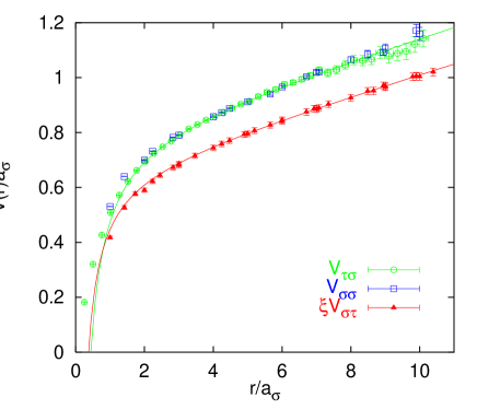
FIG. 2.: The three potentials $V_{\tau\sigma}$, $V_{\sigma\sigma}$ and $V_{\sigma\tau}$ in units of $a_{\sigma}$ at $\beta=6.2$, $\xi_{0}=3.25$.

FIG. 3.: Differences between $\hat{V}_{\sigma\sigma}$ and $\xi\hat{V}_{\sigma\tau}$.

TABLE VI.: Fits to $V_{\sigma\tau}$. The fit parameters are displayed in units of $a_{\sigma}$.

$\beta$	$L_{\sigma}$	$t_{\min}/a_{\tau}$	$r_{\min}/a_{\sigma}$	$\hat{V}_{0,\sigma\tau}\xi$	$e_{\sigma\tau}\xi$	$K_{\sigma\tau}\xi$
5.8	8	13	$\sqrt{5}$	0.756(50)	0.348(74)	0.138(8)
5.8	12	13	$\sqrt{5}$	0.732(55)	0.298(80)	0.145(9)
6.0	12	10–11	3	0.745(39)	0.354(80)	0.0659(41)
6.2	16	16–19	4	0.658(25)	0.249(67)	0.0376(17)

Assigning the phenomenological value [65, 71, 72, 70] $0.5$ fm to $r_{0}$ we find $L_{\sigma}a_{\sigma}\approx 1.3$ fm on the small lattices and $L_{\sigma}a_{\sigma}\approx 2$ fm on the $12^{3}$ lattice at $\beta=5.8$. This means that $\sqrt{3}L_{\sigma}a_{\sigma}/2>1.1$ fm in all our simulations; along the ${\mathbf{R}}\parallel(1,1,1)$ direction we are safe from the effect of mirror charges up to distances bigger than one fm. Beyond this distance only representations with non-zero triality are protected by the centre symmetry [70] from direct finite size effects.

In Fig. 2 we display all three potentials in units of $a_{\sigma}$ at $\beta=6.2$. Note that the anisotropy has been determined by matching $V_{\tau\sigma}$ to $V_{\sigma\sigma}$ at $r=4\,a_{\sigma}$. In addition to the data points two curves are included that correspond to the parameter values of Table III and Table VI from fits according to Eq. (32) to $V_{\tau\sigma}$ for $r>2a_{\sigma}$ and to $V_{\sigma\tau}$ for $r\geq 4a_{\sigma}$, respectively. The matched potentials $V_{\sigma\sigma}$ and $V_{\tau\sigma}$ follow the same curve.

Up to lattice artefacts and the self energy shift $\Delta\hat{V}_{\mbox{self}}$, $\xi\hat{V}_{\sigma\tau}$ and $\hat{V}_{\sigma\sigma}$, that both live along coarse grained lattice directions, should also agree with each other [Eq. (29)]. Indeed, as is demonstrated in Fig. 3, the differences are compatible with constants of the order suggested by tree level perturbation theory for $\xi=\xi_{0}=4$, Eq. (30). Averaging the $R\geq R_{m}^{L}$ data points results in the values, $0.091(9)$, $0.096(18)$ and $0.124(11)$ for $\Delta\hat{V}_{\mbox{self}}$ at $\beta=5.8,6.0$ and 6.2, respectively (solid lines with error bands). On the large lattice at $\beta=5.8$ we obtain the value $0.081(9)a_{\sigma}^{-1}$, in agreement with that above, from the smaller volume. These shifts of the self energies result in reduced relative errors of $\langle W_{\sigma\tau}\rangle$ [Eq. (7)] (and in increased errors of $\langle W_{\sigma\sigma}\rangle$), relative to the isotropic case.

IV The potentials

The potentials in non-fundamental representations are extracted in the same way as discussed above from fits to the corresponding smeared Wilson loops. These are obtained from the fundamental ones by use of Eqs. (11) – (19). In the case of the fundamental Wilson loops, discussed in Sec. III, temporal links have been replaced by their thermal averages in the vicinity of the surrounding staples in order to reduce statistical fluctuations [71, 73] (link integration [74]). Note that our use of Eqs. (11) – (19) implies that we cannot thermally average fundamental links in the construction of higher representation Wilson loops anymore.

We determine the potentials from correlated exponential fits to $\langle W_{D,\sigma\tau}\rangle$ data according to Eq. (6). The fit range in $T$ is selected separately for each distance ${\mathbf{R}}$ and representation $D$, such that $\chi^{2}/N_{DF}<1.5$. In addition, we demand the saturation of “effective masses”, $V_{D}(T)a_{\sigma}=\frac{\xi}{4}\ln[\langle W_{D}(T)\rangle/\langle W_{D}(T+4)\rangle]$, into plateaus for $T\geq T_{\min}$. In Table VII we display the resulting fit ranges $T\in[T_{\min},T_{\max}]$ that have been selected by means of this procedure for the example of the point $\hat{V}_{D}({\mathbf{R}})$ with $R\approx r_{0}/a_{\sigma}$. In general, the interplay between statistical errors and ground state overlaps was such that $T_{\min}$ only slightly varied with $R$. In the case of the fundamental potential we find values $2\,r_{0}\leq t_{\min}\leq 4.5\,r_{0}$, depending on $R$ and the parameter values we simulate at, while for $D={\mathbf{1}}{\mathbf{5}}{\mathbf{s}}$ we find, $0.7\,r_{0}\leq t_{\min}\leq r_{0}$. The corresponding estimated ground state overlaps $c_{D}$ are displayed in Table VIII. The overlaps decrease with increasing Casimir constant, lattice spacing or distance $r$. At $r\approx r_{0}$ the overlaps range from $0.62(3)$ in the worst case to $0.97(1)$ in the best case which quantifies the efficiency of our smearing algorithm.

In Fig. 4 we display the resulting potentials at $\beta=6.2$. The curves correspond to the three parameter fit Eq. (32) to the fundamental potential, multiplied by the respective ratio of Casimir factors, $d_{D}$ of Table I. It is clear that the Casimir scaling hypothesis Eq. (10) works quite well on our $\beta=6.2$ data for the investigated distances. In Figs. 5 – 7 we display the ratios $\hat{V}_{D}(R,a_{\sigma})/\hat{V}_{F}(R,a_{\sigma})$ for our three lattice spacings. We did not attempt to subtract the self energy contributions [cf. Eqs. (1) – (2)] in this comparison. At $\beta=5.8$ and $\beta=6.0$ we find the data to lie significantly below the corresponding Casimir ratios (horizontal lines). However, the deviations decrease rapidly as the lattice spacing is reduced.

TABLE VII.: Fit ranges $t_{\min}/a_{\tau}$ – $t_{\max}/a_{\tau}$ at $r\approx r_{0}$.

$D$	$\beta=5.8$	$\beta=6.0$	$\beta=6.2$
3	13 – 24	10 – 36	16 – 40
8	7 – 12	9 – 18	10 – 20
6	7 – 12	8 – 18	10 – 20
15a	6 – 11	6 – 14	8 – 15
10	5 – 10	5 – 11	6 – 12
27	4 – 8	4 – 8	5 – 9
24	4 – 8	4 – 8	5 – 9
15s	3 – 7	3 – 7	4 – 7

TABLE VIII.: Ground state overlaps $c_{D}$ at $r\approx r_{0}$.

$D$	$\beta=5.8$	$\beta=6.0$	$\beta=6.2$
3	0.89 (1)	0.96 (1)	0.97 (1)
8	0.81 (1)	0.90 (3)	0.91 (2)
6	0.80 (2)	0.90 (3)	0.90 (3)
15a	0.68 (4)	0.84 (3)	0.88 (5)
10	0.62 (3)	0.82 (2)	0.89 (3)
27	0.67 (3)	0.81 (2)	0.88 (3)
24	0.65 (3)	0.77 (2)	0.90 (4)
15s	0.66 (3)	0.79 (2)	0.86 (3)

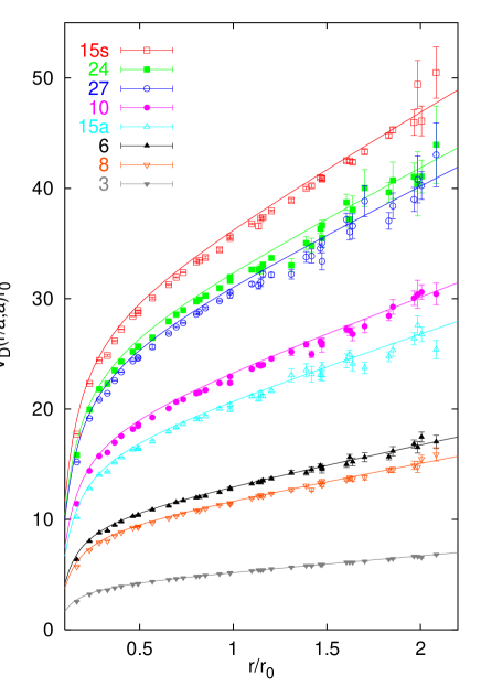
FIG. 4.: The potentials for all measured representations, obtained at $\beta=6.2$. Note that we did not subtract any self energy pieces but just rescaled the raw lattice data in units of $r_{0}$.

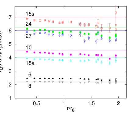
FIG. 5.: The potentials normalised to the fundamental potential at $\beta=5.8$, in comparison to the expectations from Casimir scaling (horizontal lines).

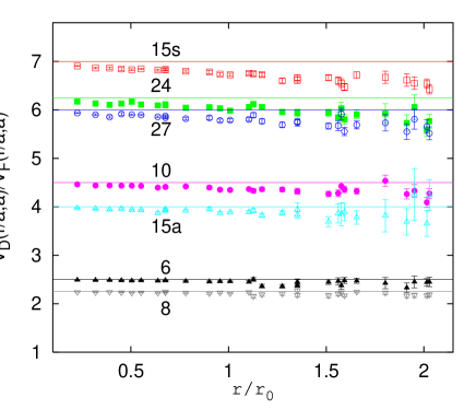
FIG. 6.: The same as Fig. 5 at $\beta=6.0$.

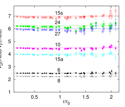
FIG. 7.: The same as Fig. 5 at $\beta=6.2$.

Prior to a continuum limit extrapolation of the ratios we shall investigate finite size effects by comparing results obtained on the 1.3 fm lattice with results from the 2 fm lattice at $\beta=5.8$. For the fundamental potential we already know from previous studies that for spatial extents, $L_{\sigma}a_{\sigma}>2\,r_{0}$, such effects are well below the 2 % level [23]. The situation is less clear for potentials in higher representations. In principle, the flux tube between the sources could widen when the energy per unit length is increased and, therefore, higher representation potentials might be more susceptible to finite size effects.

In Fig. 8 we compare the fundamental, octet and sextet potentials obtained on the $12^{3}$ lattices at $\beta=5.8$ (full symbols) with those obtained on the $8^{3}$ lattices (open symbols). Up to distances well beyond $2\,r_{0}\approx 6\,a_{\sigma}$ no statistically significant deviations are seen. In Fig. 9 we show the relative deviations, $V^{L_{\sigma}=12}_{D}({\mathbf{r}})/V^{L_{\sigma}=8}_{D}({\mathbf{r}})-1$, between the potentials determined on the larger lattices and those measured on the smaller lattices for all the representations that we have investigated. Again, no systematic or statistically significant differences are detected. Up to $r=4\,a_{\sigma}\approx 1.4\,r_{0}$ this holds true on the 1 % level for the fundamental potential and on the 3–5 % level for higher representation potentials. Beyond this distance the statistical errors start to explode. The same comparison has been performed for ratios of potentials. In this case the relative errors are slightly reduced due to correlation effects. However, no statistically significant tendencies were observed either. The relative statistical errors on the two lattices are of about the same size and comparable to those of the $\beta=6.0$ and $\beta=6.2$ simulations. Thus, we do not expect finite size effects to exceed the statistical errors on any of the simulated lattice volumes.

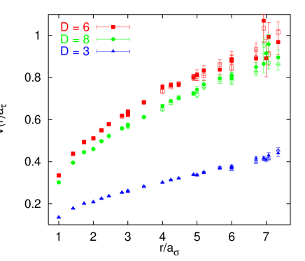
FIG. 8.: Comparison between the potentials in the lowest dimensional three representations between the $L_{\sigma}=8$ lattices (open symbols) and $L_{\sigma}=12$ lattices (full symbols) at $\beta=5.8$ in lattice units.

We now attempt a continuum limit extrapolation of our data. We remark that in the limit $a_{\sigma}\rightarrow 0$ [Eqs. (1) – (2)] the Casimir scaling of the diverging self energies $\hat{V}_{D,\mbox{self}}(a_{\sigma})$ automatically implies Casimir scaling of $\hat{V}_{D}({\mathbf{R}},a_{\sigma})$. However, with $V_{D,\mbox{self}}$ being a purely ultra violet quantity, this sort of Casimir scaling has little to do with non-perturbative aspects of the theory. As can be seen from Fig. 4, where the potentials vary by more than a factor two with the distance, even at our finest lattice resolution $V_{D,\mbox{self}}$ have not yet become the dominant contributions to the lattice potentials. In order to avoid the trivial Casimir scaling described above we will only study ratios of physical interaction energies,

$$R_{D}(r)=\frac{V_{D}(r)}{V_{F}(r)}=\frac{\hat{V}_{D}({\mathbf{R}},a_{\sigma})-\hat{V}_{D,\mbox{self}}(a_{\sigma})}{\hat{V}_{F}({\mathbf{R}},a_{\sigma})-\hat{V}_{F,\mbox{self}}(a_{\sigma})}\left[1+{\mathcal{O}}(a_{\sigma}^{2})\right],$$ (34)

where $r=Ra_{\sigma}$.

FIG. 9.: Relative deviations $V^{L_{\sigma}=12}_{D}({\mathbf{r}})/V^{L_{\sigma}=8}_{D}({\mathbf{r}})-1$ of the potentials obtained on different volumes as a function of $r/a_{\sigma}$.

We estimate the self energies in leading order perturbation theory, Eq. (8). Lattice perturbation theory is notorious for its bad convergence behaviour [24, 68]. However, in our anisotropic case the effective expansion parameter $g^{2}\xi_{0}^{-1}$ is much smaller than in standard applications of lattice perturbation theory. In Fig. 3 we have indeed seen that leading order perturbation theory predictions on the difference of two self energies agree within 30 % with numerical data. We estimate the self energies in two different ways: (a) we use the bare lattice coupling and the renormalised anisotropy $\xi$, (b) we mean field (“tadpole”) improve [67, 68] both, coupling and anisotropy [Eq. (33)], $\xi_{0,ir}^{-1}g^{2}_{ir}=\xi_{0}^{-1}g^{2}\langle U_{\sigma\tau}\rangle^{-1}$. The results from the two methods, shown in Table IX, differ by up to 60 % from each other. We will use the estimate (a) in our analysis but take the difference between (a) and (b) into account as a systematic error. While data at large distances are marginally affected by this uncertainty, the error bars at small distances are significantly increased.

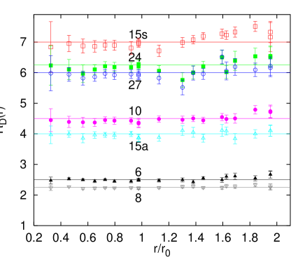
FIG. 10.: Continuum limit extrapolated ratios, Eq. (34), compared to the Casimir scaling hypothesis (horizontal lines).

After subtracting the (scaling violating) self energy contributions we determine the continuum extrapolated ratios $R_{D}(r)$ by means of quadratic fits, Eq. (34). We perform these extrapolations for all the distances $r$ that have been realised on our coarsest lattice ($\beta=5.8$) in units of $r_{0}$. On the finer lattices, we linearly interpolate between the two lattice points that are closest to each given distance $r$, prior to the quadratic continuum limit fit. We find the data to be compatible with the quadratic ansatz and the resulting ratios are shown in Fig. 10. The numerical values are displayed in Tables X – XI. No statistically significant violations of Casimir scaling are found. Our accuracy is somewhat limited at short distances, due to the perturbative estimation of the self energies. The slope of the extrapolation in $a_{\sigma}^{2}$ increases with the distance $r$ as well as with the Casimir charge $C_{D}$; large masses $\hat{V}_{D}(R,a_{\sigma})>a_{\tau}^{-1}$ are more affected by lattice artefacts than small masses. This observation also explains why the deviations from Casimir scaling at $\beta=5.8$ and $\beta=6.0$ increase with the distance (Figs. 5 – 6).

TABLE IX.: Perturbative estimates of the self energy $\hat{V}_{F,\mbox{self}}$ (in units of $a_{\tau}$).

$\beta$	bare $g^{2}$, renormalised $\xi$	mean field $g_{ir}^{2}\xi_{0,ir}^{-1}$
5.8	0.0855(05)	0.13931
6.0	0.0825(15)	0.12835
6.2	0.0824(11)	0.12093

TABLE X.: The continuum ratios, $R_{D}(r)=V_{D}(r)/V_{F}(r)$. “exp.” denotes the Casimir scaling expectation.

$r/r_{0}$	$D=8$	$D=6$	$D=15a$
0.33	2.24(09)	2.48(11)	3.97(29)
0.46	2.27(03)	2.53(04)	3.99(10)
0.56	2.21(04)	2.50(04)	3.86(15)
0.65	2.23(04)	2.45(05)	3.96(11)
0.73	2.24(02)	2.50(03)	3.97(08)
0.80	2.23(03)	2.45(04)	3.95(11)
0.92	2.24(03)	2.45(05)	4.00(08)
0.98	2.23(04)	2.50(05)	3.87(12)
0.98	2.22(04)	2.49(04)	3.85(11)
1.13	2.24(04)	2.48(05)	3.88(12)
1.30	2.27(05)	2.49(07)	4.11(16)
1.38	2.28(04)	2.43(07)	4.05(16)
1.45	2.24(04)	2.55(05)	3.86(13)
1.59	2.24(05)	2.49(08)	4.11(19)
1.63	2.29(05)	2.60(08)	4.09(13)
1.69	2.28(06)	2.61(10)	3.84(17)
1.84	2.33(06)	2.55(09)	4.00(14)
1.95	2.26(10)	2.67(12)	4.10(19)
1.95	2.27(09)	2.66(11)	4.10(18)
2.18	2.30(11)	2.11(16)	3.67(26)
2.25	1.97(16)	2.03(20)	3.41(43)
2.30	2.26(14)	2.45(17)	3.72(31)
2.39	2.29(14)	2.46(16)
exp.	2.25	2.5	4

TABLE XI.: The same as Table X for higher representations.

$r/r_{0}$	$D=10$	$D=27$	$D=24$	$D=15s$
0.33	4.45(37)	6.23(65)	5.98(57)	6.84(83)
0.46	4.39(18)	6.10(33)	5.94(22)	6.95(27)
0.56	4.38(16)	5.96(29)	5.82(23)	6.87(23)
0.65	4.37(13)	6.10(16)	5.86(14)	6.86(19)
0.73	4.45(11)	6.21(15)	5.97(14)	6.90(17)
0.80	4.43(12)	6.18(16)	5.92(14)	6.89(17)
0.92	4.43(10)	6.17(16)	5.95(14)	6.81(21)
0.98	4.34(14)	6.28(14)	5.95(15)	7.00(13)
0.98	4.37(14)	6.21(12)	5.91(14)	6.95(12)
1.13	4.48(10)	6.06(17)	5.82(19)	6.71(19)
1.30	4.46(11)	5.76(24)	5.52(24)	6.99(16)
1.38	4.50(10)	6.00(21)	5.99(23)	7.08(14)
1.45	4.44(10)	6.21(16)	5.96(18)	7.19(12)
1.59	4.55(12)	6.50(23)	6.52(23)	7.27(15)
1.63	4.48(13)	6.02(21)	6.05(29)	7.23(14)
1.69	4.50(16)	6.39(31)	6.19(28)	7.33(17)
1.84	4.79(14)	6.53(27)	6.09(22)	7.51(16)
1.95	4.74(20)	6.51(33)	6.21(30)	7.16(48)
1.95	4.71(19)	6.54(32)	6.16(29)	7.33(35)
2.18	4.40(36)	5.93(53)	5.89(43)	7.19(57)
2.25	3.12(50)	5.67(71)	5.99(58)
2.30	3.82(44)	6.37(76)	5.97(53)
2.39	3.62(53)
exp.	4.5	6	6.25	7

V Discussion

We have confirmed that violations of the Casimir scaling hypothesis,

$$\frac{V_{D_{1}}(r)}{V_{D_{2}}(r)}=\frac{C_{D_{1}}}{C_{D_{2}}},$$ (35)

are below the 5 % level for distances $r<2\,r_{0}\approx 1$ fm in the continuum limit of four dimensional $SU(3)$ gauge theory for all representations with $C_{D}\leq 7$. This finding rules out many models of non-perturbative QCD and imposes serious restrictions onto others. For instance in a bag model calculation scaling of string tensions with the square root of the respective Casimir ratio has been obtained [75] and instanton liquid calculations result in ratios between potentials in different representations that are smaller than the Casimir ratios too [76].

Another possibility would have been scaling proportional to the number of fundamental flux tubes embedded into the higher representation vortex [$p+q$ in $SU(3)$] [39, 41], which happens to coincide with Casimir scaling in the large $N$ limit of $SU(N)$. This picture is supported by the finding that the $SU(N)$ vacuum seems to act like a type I superconductor [77, 78], i.e. flux tubes repel each other. However, this scenario is also excluded by the present study. Furthermore, serious restrictions onto most of the remaining models are imposed (see for instance Ref. [51]). It is particularly disappointing that neither centre vortex models [47, 48, 49] nor the dual superconductor scenario [79, 80, 78] or string models [11] seem to offer any explanation why the numerical data so closely resemble the Casimir ratios. Certainly, it is worthwhile to dedicate more theoretical effort to this fundamental phenomenon.

We have not discussed “string breaking” so far. While the fundamental potential in pure gauge theories linearly rises ad infinitum, the adjoint potential will be screened by gluons and, at sufficiently large distances, decay into two disjoint gluelumps [81, 39, 70]. This string breaking has indeed been confirmed in numerical studies [44, 45, 27, 28, 35]. Therefore, strictly speaking, the adjoint string tension is zero. In fact, all charges in higher than the fundamental representation will be at least partially screened by the background gluons. For instance, ${\mathbf{6}}\otimes{\mathbf{8}}={\mathbf{2}}{\mathbf{4}}\oplus{\mathbf{1}}{\mathbf{5}}{\mathbf{a}}^{*}\oplus{\mathbf{6}}\oplus{\mathbf{3}}^{*}$: in interacting with the glue, the sextet potential obtains a fundamental component. A simple rule, related to the centre of the group, is reflected in Eqs. (11) – (19): wherever $z^{p-q}=1$ (zero triality), the source will be reduced into a singlet component at large distances while, wherever $z^{p-q}=z$ (or $z^{*}$), it will be screened, up to a residual (anti-)triplet component, i.e. one can easily read off the asymptotic string tension (either zero or the fundamental string tension) from the third column of Table I, rather than having to multiply and reduce representations. As a result, the self-adjoint representations, ${\mathbf{8}}$ and ${\mathbf{2}}{\mathbf{7}}$, as well as the representation, ${\mathbf{1}}{\mathbf{0}}$, will be completely screened while in all other representations with $p+q\leq 4$ a residual fundamental component survives. The same argument, applied to $SU(2)$, results in the prediction that all odd-dimensional (bosonic) representations are completely screened while all even-dimensional (fermionic) representations will tend towards the fundamental string tension at large distances.

One expects this sort of string breaking and flattening of the potential to occur at distances larger than about 2.4 $r_{0}$ [39]. Obviously, once the string is broken Casimir scaling is violated. It is certainly interesting to investigate what happens around the string breaking distance. However, this requires lattice volumes exceeding those used in the present study as well as additional operators that are designed for an optimal overlap with the respective broken string states [82].

- [1] A. Chodos, R. L. Jaffe, K. Johnson, C. B. Thorn, and V. F. Weisskopf, Phys. Rev. D9, 3471 (1974).
- [2] T. DeGrand, R. L. Jaffe, K. Johnson, and J. Kiskis, Phys. Rev. D12, 2060 (1975).
- [3] P. Hasenfratz and J. Kuti, Phys. Rept. 40, 75 (1978).
- [4] C. E. DeTar and J. F. Donoghue, Ann. Rev. Nucl. Part. Sci. 33, 235 (1983).
- [5] K. J. Juge, J. Kuti and C. J. Morningstar, Nucl. Phys. Proc. Suppl. 63, 543 (1998) [hep-lat/9709132].
- [6] J. Kogut, D. K. Sinclair, and L. Susskind, Nucl. Phys. B114, 199 (1976).
- [7] W. Buchmüller, Phys. Lett. 112B, 479 (1982).
- [8] N. Isgur and J. Paton, Phys. Lett. 124B, 247 (1983).
- [9] N. Isgur and J. Paton, Phys. Rev. D31, 2910 (1985).
- [10] P. Goddard, J. Goldstone, C. Rebbi, and C. B. Thorn, Nucl. Phys. B56, 109 (1973).
- [11] M. Lüscher, G. Münster, and P. Weisz, Nucl. Phys. B180, 1 (1981).
- [12] H. G. Dosch, Phys. Lett. B190, 177 (1987).
- [13] H. G. Dosch and Yu. A. Simonov, Phys. Lett. 205B, 339 (1988).
- [14] Yu. A. Simonov, Nucl. Phys. B307, 512 (1988).
- [15] M. Baker, J. S. Ball, and F. Zachariasen, Nucl. Phys. B229, 445 (1983).
- [16] M. Baker, J. S. Ball, and F. Zachariasen, Phys. Rev. D51, 1968 (1995).
- [17] M. Baker, J. S. Ball, N. Brambilla, G. M. Prosperi, and F. Zachariasen, Phys. Rev. D54, 2829 (1996) [hep-ph/9602419], erratum, ibid. D56, 2475 (1997).
- [18] S. Maedan and T. Suzuki, Prog. Theor. Phys. 81, 229 (1989).
- [19] M. N. Chernodub, S. Kato, N. Nakamura, M. I. Polikarpov and T. Suzuki, [hep-lat/9902013].
- [20] E. V. Shuryak, Nucl. Phys. B203, 93 (1982).
- [21] D. I. Diakonov and V. Y. Petrov, Nucl. Phys. B272, 457 (1986).
- [22] T. Schäfer and E. V. Shuryak, Rev. Mod. Phys. 70, 323 (1998) [hep-ph/9610451].
- [23] G. S. Bali and K. Schilling, Phys. Rev. D46, 2636 (1992).
- [24] G. S. Bali and K. Schilling, Phys. Rev. D47, 661 (1993) [hep-lat/9208028].
- [25] J. Ambjørn, P. Olesen, and C. Peterson, Nucl. Phys. B240, 533 (1984).
- [26] G. I. Poulis and H. D. Trottier, Phys. Lett. B400, 358 (1997) [hep-lat/9504015].
- [27] P. W. Stephenson, Nucl. Phys. B550, 427 (1999) [hep-lat/9902002].
- [28] O. Philipsen and H. Wittig, Phys. Lett. B451, 146 (1999) [hep-lat/9902003].
- [29] C. Bernard, Phys. Lett. 108B, 431 (1982).
- [30] C. Bernard, Nucl. Phys. B219, 341 (1983).
- [31] J. Ambjørn, P. Olesen, and C. Peterson, Nucl. Phys. B240, 189 (1984).
- [32] C. Michael, Nucl. Phys. B259, 58 (1985).
- [33] L. A. Griffiths, C. Michael, and P. E. L. Rakow, Phys. Lett. 150B, 196 (1985).
- [34] H. D. Trottier, Phys. Lett. B357, 193 (1995) [hep-lat/9503017].
- [35] P. de Forcrand and O. Philipsen, Phys. Lett. B475, 280 (2000) [hep-lat/9912050].
- [36] K. Kallio and H. D. Trottier, (2000) [hep-lat/0001020].
- [37] N. A. Campbell, I. H. Jorysz, and C. Michael, Phys. Lett. 167B, 91 (1986).
- [38] C. Michael, Nucl. Phys. Proc. Suppl. 26, 417 (1992).
- [39] C. Michael, (1998) [hep-ph/9809211].
- [40] S. Deldar, Nucl. Phys. Proc. Suppl. 73, 587 (1999) [hep-lat/9809137].
- [41] G. S. Bali, Nucl. Phys. Proc. Suppl. 83-84, 422 (2000) [hep-lat/9908021].
- [42] S. Deldar, Phys. Rev. D62, 034509 (2000) [hep-lat/9911008].
- [43] S. Ohta, M. Fukugita, and A. Ukawa, Phys. Lett. B173, 15 (1986).
- [44] H. Markum and M. E. Faber, Phys. Lett. B200, 343 (1988).
- [45] M. Müller, W. Beirl, M. Faber, and H. Markum, Nucl. Phys. Proc. Suppl. 26, 423 (1992).
- [46] W. Buerger, M. Faber, H. Markum, and M. Müller, Phys. Rev. D47, 3034 (1993).
- [47] M. Faber, J. Greensite and S. Olejnik, Phys. Rev. D57, 2603 (1998) [hep-lat/9710039].
- [48] J. M. Cornwall, Phys. Rev. D57, 7589 (1998) [hep-th/9712248].
- [49] S. Deldar, [hep-ph/9912428].
- [50] Yu. A. Simonov, JETP Lett. 71, 127 (2000) [hep-ph/0001244].
- [51] V. I. Shevchenko and Yu. A. Simonov, [hep-ph/0001299].
- [52] K. G. Wilson, Phys. Rev. D10, 2445 (1974).
- [53] APE, M. Albanese et al., Phys. Lett. 192B, 163 (1987).
- [54] G. S. Bali, K. Schilling, and C. Schlichter, Phys. Rev. D51, 5165 (1995) [hep-lat/9409005].
- [55] P. Altevogt and F. Gutbrod, Nucl. Phys. B452, 649 (1995).
- [56] F. Karsch, Nucl. Phys. B205, 285 (1982).
- [57] P. Weisz and R. Wohlert, Nucl. Phys. B236, 397 (1984).
- [58] Y. Schröder, Phys. Lett. B447, 321 (1999) [hep-ph/9812205].
- [59] T. R. Klassen, Nucl. Phys. B533, 557 (1998) [hep-lat/9803010].
- [60] S. Ejiri, Y. Iwasaki and K. Kanaya, Phys. Rev. D58, 094505 (1998) [hep-lat/9806007].
- [61] J. Engels, F. Karsch and T. Scheideler, Nucl. Phys. B564, 303 (2000) [hep-lat/9905002].
- [62] N. Cabibbo and E. Marinari, Phys. Lett. B119, 387 (1982).
- [63] K. Fabricius and O. Haan, Phys. Lett. B143, 459 (1984).
- [64] M. Creutz, Phys. Rev. D36, 515 (1987).
- [65] R. Sommer, Nucl. Phys. B411, 839 (1994) [hep-lat/9310022].
- [66] M. Garcia Perez and P. van Baal, Phys. Lett. B392, 163 (1997) [hep-lat/9610036].
- [67] G. Parisi, in Proc. of the 20th Int. Conf. on High Energy Physics, Madison, Jul 17-23, 1980, eds. L. Durand and L.G. Pondrom, (American Inst. of Physics, New York, 1981).
- [68] G. P. Lepage and P. B. Mackenzie, Phys. Rev. D48, 2250 (1993) [hep-lat/9209022].
- [69] K. Schilling and G. S. Bali, Int. J. Mod. Phys. C4, 1167 (1993) [hep-lat/9308014].
- [70] G. S. Bali, Phys. Rept. in print [hep-ph/0001312].
- [71] G. S. Bali, K. Schilling, and A. Wachter, Phys. Rev. D56, 2566 (1997) [hep-lat/9703019].
- [72] G. S. Bali and P. Boyle, Phys. Rev. D59, 114504 (1999) [hep-lat/9809180].
- [73] P. De Forcrand and C. Roiesnel, Phys. Lett. B151, 77 (1985).
- [74] G. Parisi, R. Petronzio and F. Rapuano, Phys. Lett. B128, 418 (1983).
- [75] K. Johnson and C. B. Thorn, Phys. Rev. D13, 1934 (1976).
- [76] D. Diakonov, V. Y. Petrov and P. V. Pobylitsa, Phys. Lett. B226, 372 (1989).
- [77] G. S. Bali, C. Schlichter, and K. Schilling, Prog. Theor. Phys. Suppl. 131, 645 (1998) [hep-lat/9802005].
- [78] G. S. Bali, (1998) [hep-ph/9809351].
- [79] G. S. Bali, V. Bornyakov, M. Muller-Preussker and K. Schilling, Phys. Rev. D54, 2863 (1996) [hep-lat/9603012].
- [80] J. Ambjørn and J. Greensite, JHEP 9805, 004 (1998) [hep-lat/9804022].
- [81] I. H. Jorysz and C. Michael, Nucl. Phys. B302, 448 (1988).
- [82] K. Schilling, Nucl. Phys. Proc. Suppl. 83-84, 140 (2000) [hep-lat/9909152].