BUTP/2000-15

Unexpected results in asymptotically free quantum field theories

Peter Hasenfratz and Ferenc Niedermayer

Institute for Theoretical Physics

University of Bern

Sidlerstrasse 5, CH-3012 Bern, Switzerland

Abstract

We study the behavior of asymptotically free (AF) spin and gauge models when their continuous symmetry group is replaced by different discrete non-Abelian subgroups. Precise numerical results with relative errors down to O(0.1%) suggest that the models with large subgroups are in the universality class of the underlying original models. We argue that such a scenario is consistent with the known properties of AF theories. The small statistical errors allow a detailed investigation of the cut-off effects also. At least up to correlation lengths $\xi\approx 300$ they follow effectively an $\propto a$ rather than the expected $\propto a^{2}$ form both in the O(3) and in the dodecahedron model.

1 Introduction

AF quantum field theories are relevant both in particle and in condensed matter physics. Their standard formulation is based on a global ($d=2$ spin models), or local ($d=4$ gauge theories) non-Abelian continuous symmetry group. In this work we discuss a scenario which, beyond its field theoretical interest, might open new analytic and numerical ways to study such theories.

Lattice regularization allows (both in spin and gauge models) to replace the continuous symmetry group by one of its finite discrete non-Abelian subgroups. The new model has a reduced symmetry and, due to the discreteness of the group, a finite action gap. If the bare coupling constant $g$ is large, then the fluctuations are large and these new features of the model will have a small effect. At small $g$, however, the finite action gap kills the fluctuations and the system will be frozen. We expect therefore a phase transition between the strong and weak coupling regions - possibly even two transitions, if there is a massless phase between them. As opposed to that, the original AF model is expected to have a single phase only approaching the continuum limit as $g\rightarrow 0$.

Denote the phase transition point at the end of the strong coupling phase of the discrete subgroup model by $g_{c}$ and assume that the transition is second order. (We shall discuss the case of a first order transition later.) We suggest that the quantum field theory obtained in the limit $g\searrow g_{c}$ is in the same universality class as the original AF model if the subgroup is sufficiently large.

In the early 80’s gauge models on discrete non-Abelian subgroups were introduced as an approximation to the SU(2) Yang-Mills theory [1]. That time it was considered as obvious that this is an approximation only since the Wilson loop expectation values measured at some coupling $g$ were different. Our suggestion above, however, refers to the situation when the discrete and continuous group models are compared at the same large correlation length (approaching the continuum limit) for physical quantities.

A nice example, where a discrete internal symmetry of the action is elevated to a continuous symmetry, is the d=2 XY model. Considering perturbations which break the O(2) symmetry down to Z($N$) in the massless low temperature phase, for $g>g(N)$ the discrete symmetry is elevated to full O(2) in the long distance predictions if $N>4$ [2]. Our case is more complicated since AF theories have a non-perturbative finite mass gap.

We were inspired to investigate models with discrete subgroups through the observations made by Patrascioiu and Seiler a few years ago [3] who noticed that, within the statistical errors, the physical results of the dodecahedron spin model for $g>g_{c}$ are consistent with that of the O(3) non-linear $\sigma$-model. They concluded that the O(3) model should also have a phase transition and so, none of the two models is AF. We believe that overwhelming evidence exists that the O(3) $\sigma$-model is AF and our suggestion implies that the dodecahedron model is also AF. This statement should be understood in the sense that the physical running coupling goes to zero as the corresponding momentum scale goes to infinity.

If our suggestion is correct, the relation between the bare coupling of the original model and that of its discrete subgroup version is non-analytic. The standard arguments which demonstrate the universality of the first two terms in the beta function describing the change of the bare coupling under the change of the cut-off are not valid.

There exists a special class of non-Abelian subgroups, the dihedral subgroups of SU(N) which are not considered in this work. (The discrete subgroups of SU(3) are discussed in Ref. [4].) These subgroups can be made arbitrarily large and, although they do not go over to SU(N) in this limit, the action gap gets arbitrarily small. Due to the fact that they inherit some of those properties of SU(N) which are thought to be relevant for confinement in the Yang-Mills theory, Kaplan raised the possibility that they are in the universality class of SU(N) [5]. It would be interesting to investigate this scenario also.

2 AF spin models in $d=2$

We studied discrete spin models where the symmetry group is one of the non-Abelian subgroups of O(3). These subgroups are the symmetry groups of regular polyhedra. Embedding the regular polyhedron in $S_{2}$ the corners define the discrete directions of the unit spin ${\bf S}(x)$. We shall refer to the discrete spin model by the name of the corresponding polyhedron. For all the subgroups we used the standard nearest-neighbor action.

We found that the spin models with small subgroups (tetrahedron, octahedron and cube with 4, 6 and 8 directions, respectively) are definitely not equivalent to the O(3) non-linear $\sigma$-model. The two largest subgroups (icosahedron and dodecahedron with 12 and 20 directions, respectively) could not be distinguished from the O(3) $\sigma$-model, however. In particular, for the dodecahedron the agreement is established on the level of O(0.1%).

It is easy to show that the tetrahedron model is identical to the $q=4$ Potts model with $\beta_{{\rm tetra}}=3/4\beta_{{\rm Potts}}^{q=4}$, where $\beta=1/g$. Similarly, the cube model is the product of 3 independent Ising models. This is obvious if one takes the 8 vectors pointing to the corners of the cube as $1/\sqrt{3}(\pm 1,\pm 1,\pm 1)$. Then the cube action becomes a sum of 3 independent Ising actions, with the relation $\beta_{\rm cube}=3\beta_{\rm Ising}$ between the corresponding couplings. A lot is known about the $q=4$ Potts and the Ising model and we can certainly exclude that they are in the universality class of the O(3) $\sigma$-model.

We have chosen physical quantities which can be measured precisely: the finite-size scaling function, the renormalized zero momentum 4-point coupling $g_{\rm R}$ and the same coupling in a finite physical volume. It is the latter quantity which can be measured with the highest precision.

2.1 The finite-size scaling function

An $L\times L$ periodic box is considered and the second moment correlation length $\xi(L)$ is measured. The relative change of the correlation length when $L$ is doubled, $\xi(2L)/\xi(L)$ is studied as the function of $\xi(L)/L$. Both these ratios are physical quantities if $L$ and $\xi(L)$ are much larger than the lattice unit $a$. The finite-size scaling function is a valuable tool to connect the small and large volume regimes[6]. This technique has been used very effectively by Lüscher, Weisz and Wolff[7] in their study of the running coupling in the O(3) model. The finite-size scaling function has been measured precisely by Caracciolo et al.[8] in the same model for a large set of $\xi(L)/L$ values, using the second-moment correlation length. The latter is defined in an $L\times L$ box as

$$\xi(L)=\frac{1}{2\sin(\pi/L)}\sqrt{\frac{G_{2}(0)}{G_{2}(k_{0})}-1}\,,$$ (1)

where $G_{2}(k)$ is the 2-point spin correlation function in Fourier space and $k_{0}=(2\pi/L,0)$. The finite-size scaling function was also studied for the $q=4$ Potts model (equivalent to the tetrahedron model) by Salas and Sokal[9]. The two functions are completely, even qualitatively different. The largest deviation between the O(3) and tetrahedron finite-size scaling curves is around $\xi(L)/L=0.4$. We have decided, therefore to study this function in the neighborhood of this value for the different subgroups as the continuum limit is approached.

In Figure 1 the small neighborhood of $\xi(L)/L=0.4$ is shown only. The solid line is the O(3) finite-size scaling curve in the continuum limit [8]. Points with identical symbols belong to the same subgroup at different $L$ values. At fixed $\xi(L)/L$ the $L\rightarrow\infty$ limit is the continuum limit. The tetrahedron, octahedron and cube models deviate strongly from O(3) and the deviation grows as we move towards the continuum. The icosahedron and dodecahedron approach the O(3) and at the largest $L$ (increased size symbols) they lie on the O(3) curve within the statistical errors.

In Figure 1 the points scatter around $\xi(L)/L=0.4$. With careful tuning one might stay closer to this value, but since the scaling function describes physics at every $\xi(L)/L$ this was not necessary for the conclusion.

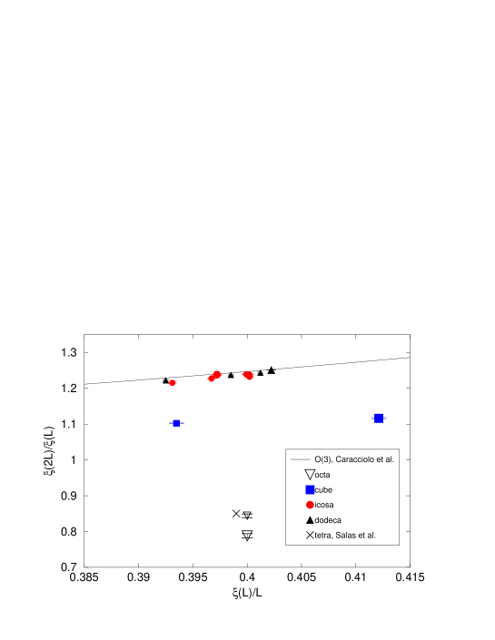
Figure 1: The $\xi(L)/L\sim 0.4$ part of the finite-size scaling curve (solid line) of the O(3) non-linear $\sigma$-model [8] is compared with the results of discrete spin models based on different non-Abelian subgroups of O(3). Points with identical symbols belong to the same subgroup at different $\xi(L)$ values. (The largest $\xi$ corresponds to a larger symbol.) The points of the icosahedron and dodecahedron models move towards the O(3) curve as the correlation length is increased and no difference beyond the statistical errors can be seen at the largest correlation length.

2.2 The renormalized zero momentum 4-point coupling $g_{\rm R}$

Define the quantity $g_{\rm R}$ as

$$g_{\rm R}=\left(\frac{L}{\xi(L)}\right)^{2}\left(1+\frac{2}{N}-\frac{\langle({\bf M}^{2})^{2}\rangle}{\langle{\bf M}^{2}\rangle^{2}}\right),$$ (2)

where $\xi(L)$ is the second moment correlation length, eq. (1), $z=L/\xi(L)$, $N=3$ for O(3) and ${\bf M}$ is the magnetization,

$$M^{a}=\sum_{x}S^{a}(x)\,.$$ (3)

The coupling $g_{\rm R}^{\infty}$ (which is denoted in the literature simply by $g_{\rm R}$) is defined as the infinite volume ($z\to\infty$) limit of $g_{\rm R}$. (It is assumed, of course, that first the continuum limit $\xi\to\infty$ is taken for fixed $z$.) For the O(3) $\sigma$-model $g_{\rm R}^{\infty}$ has been calculated using the form-factor bootstrap method: $g_{\rm R}^{\infty}=6.770(17)$ in agreement with the MC result $g_{\rm R}^{\infty}=6.77(2)$ [10].

We have measured $g_{\rm R}$ for the icosahedron and dodecahedron models for $z\sim 6$ and extrapolated to infinite volume using the finite size formula of ref. [10]. The latter was obtained from the leading $1/N$ expansion[11] applied to finite volume. Although it was derived at large $N$, as an empirical formula it works well also at N=3 [10]. Figure 2 gives the deviation from the O(3) result as the function of $\xi$. ($\xi\rightarrow\infty$ is the continuum limit). For comparison, the coupling from the cubic group is $g_{\rm R}^{{\rm cubic}}=1/3g_{\rm R}^{{\rm Ising}}$ with $g_{\rm R}^{{\rm Ising}}=14.6975(1)$ from ref.[12], i.e. for this case the deviation from O(3) is 1.87(2).

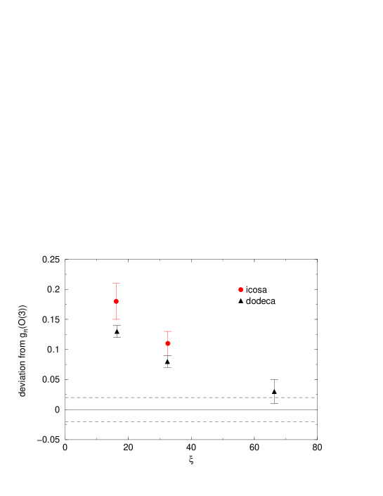
Figure 2: The deviation between the renormalized coupling of O(3) and that of the two largest subgroups as the function of the correlation length.

As Figures 1 and 2 show, the two largest non-Abelian subgroups behave qualitatively differently from the small subgroups. The results suggest that the icosahedron and dodecahedron models are in the same universality class as the O(3) non-linear $\sigma$-model.

2.3 A high precision test

We discuss now a test using a physical quantity which can be measured both in the O(3) and in the dodecahedron model to very high precision. The coupling $g_{\rm R}$ in eq. (2) is a physical quantity also in a finite physical volume, i.e. in the continuum limit keeping $z=L/\xi$ fixed. The numerical problem is much easier at some moderate value of $z$ than at large $z$. We have chosen to measure in the vicinity of the arbitrary value $z_{0}=2.32$.

For O(3) we have used the standard nearest neighbor (nn) and the parametrized fixed-point (FP) actions [13], while for the dodecahedron model the nn action was taken.

Table 1 summarizes the results for the three actions considered. The last column, $g_{\rm R}(z_{0})$ is derived from the previous column as explained below.

$L$	$\beta$	$z$	$g_{\rm R}$	$g_{\rm R}-c(z-z_{0})$	$g_{\rm R}(z_{0})$
10	1.3637	2.3199(2)	3.0103(5)	3.0105(1)	3.0105(1)
28	1.575	2.3392(3)	3.1132(6)	3.0747(2)
	1.578	2.3227(4)	3.0818(8)	3.0764(2)
	1.5785	2.3200(3)	3.0764(8)	3.0765(2)	3.0765(2)
56	1.697	2.3201(4)	3.0981(9)	3.0979(2)	3.0979(2)
	1.70	2.3030(4)	3.0650(9)	3.0984(2)
112	1.8074	2.3230(4)	3.1155(9)	3.1095(2)	3.1095(2)
	1.81	2.3073(4)	3.0843(9)	3.1096(3)
224	1.918	2.3159(5)	3.1061(13)	3.1143(3)
	1.9176	2.3178(5)	3.1099(12)	3.1144(3)	3.1145(3)
	1.9172	2.3212(5)	3.1171(11)	3.1146(3)
448	2.0276	2.3289(25)	3.1355(60)	3.1178(15)
	2.028	2.3204(10)	3.1183(23)	3.1175(6)	3.1175(6)
10	0.8562	2.3226(8)	3.1118(18)	3.1066(5)
	0.8563	2.3217(8)	3.1092(18)	3.1059(5)
	0.8565	2.3202(4)	3.1069(9)	3.1064(2)	3.1064(2)
	0.8567	2.3185(7)	3.1034(17)	3.1063(5)
	0.86	2.3050(10)	3.0767(24)	3.1067(7)
20	1.00	2.3197(5)	3.1135(9)	3.1140(3)	3.1140(3)
40	1.1347	2.3235(7)	3.1232(15)	3.1163(4)	3.1163(4)
	1.14	2.2950(20)	3.0666(44)	3.1166(11)
	1.144	2.2762(22)	3.0285(49)	3.1161(12)
80	1.25	2.4024(48)	3.2827(112)	3.1179(30)
	1.264	2.3298(16)	3.1372(36)	3.1175(9)
	1.2659	2.3199(9)	3.1178(20)	3.1180(5)	3.1180(5)
28	1.56	2.3389(9)	3.1041(22)	3.0663(7)
	1.5636	2.3177(7)	3.0639(17)	3.0685(4)	3.0683(5)
	1.565	2.3099(8)	3.0494(19)	3.0695(5)
56	1.664	2.3596(19)	3.1702(46)	3.0900(14)
	1.670	2.3190(9)	3.0905(22)	3.0924(6)	3.0923(7)
112	1.762	2.3242(10)	3.1128(23)	3.1043(6)
	1.7626	2.3211(6)	3.1072(14)	3.1051(4)	3.1051(5)
224	1.8465	2.3185(7)	3.1077(16)	3.1107(4)	3.1106(5)

Table 1: Measurements of $z=L/\xi(L)$, $g_{\rm R}$, $g_{\rm R}-c(z-z_{0})$ (with $c=2.0$ and $z_{0}=2.32$), and the extrapolated value $g_{\rm R}(z_{0})$ for the O(3) nn action, O(3) FP action and dodecahedron action, respectively. Note that the error of $g_{\rm R}-c(z-z_{0})$ is by a factor $\sim 4$ smaller than that of $g_{\rm R}$. The last column, $g_{\rm R}(z_{0})$ is obtained by extrapolating the values of $g_{\rm R}-c(z-z_{0})$ to $z=z_{0}$.

Figure 3 shows the dependence of the quantity $g_{\rm R}-c(z-z_{0})$ on $z$ around $z_{0}=2.32$ with $c=2$. The value of $g_{\rm R}(z_{0})$ is obtained by interpolating these data to $z=z_{0}$. Since $z$ was quite close to the chosen value of $z_{0}$ this procedure introduces only a small, controllable error. Similar plots for the other two actions are not shown here but could be reconstructed from Table 1.

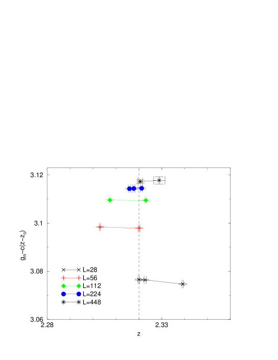
Figure 3: The quantity $g_{\rm R}-c(z-z_{0})$ vs. $z$ for the standard O(3) action with $c=2.0$ and $z_{0}=2.32$.

Figure 4 shows $g_{\rm R}(z_{0})$ as the function of $a/L$ for the three actions considered.

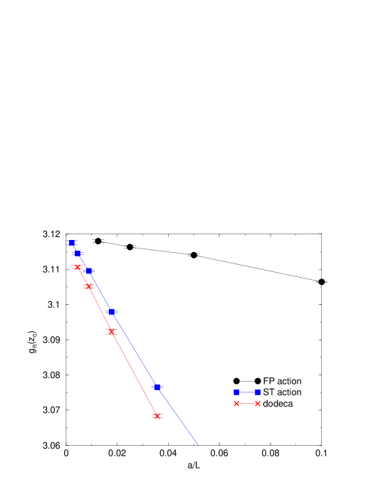
Figure 4: Cut-off dependence of $g_{\rm R}(z_{0})$ (at $z_{0}=2.32$) for the standard, FP and dodecahedron actions. The data points are connected to guide the eye.

The statistical errors of $g_{\rm R}(z_{0})$ at a given $a/L$ are quite small ($\sim 10^{-4}$ for the O(3) nn action). However, the result of the extrapolation to the continuum limit of present data depends much more on the Ansatz used. Below we present fits with different functional forms, together with the corresponding value of $\chi^{2}/{\rm dof}$:

Standard action:

$$3.1201(2)-1.224(9)a/L\,, (2.1)$$

$$3.1205(4)-1.28(5)a/L+1.1(1.1)(a/L)^{2}\,, (2.2)$$

$$3.1207(6)-1.1(1)a/L-0.04(4)a/L\log(L/a)\,, (2.5)$$

$$3.1168(3)+103(5)(a/L)^{2}-40.4(1.4)(a/L)^{2}\log(L/a)\,, (4.1)$$

FP action

$$3.1202(3)-0.137(4)a/L\,, (3.7)$$

$$3.1186(7)-0.07(3)a/L-0.5(2)(a/L)^{2}\,, (2.5)$$

$$3.1178(11)-0.23(4)a/L+0.05(2)a/L\log(L/a)\,, (1.6)$$

$$3.1180(5)+0.4(7)(a/L)^{2}-0.7(3)(a/L)^{2}\log(L/a)\,, (1.6)$$

dodecahedron action

$$3.1169(4)-1.36(2)a/L\,, (0.4)$$

$$3.1168(9)-1.4(1)a/L-0.5(3.1)(a/L)^{2}\,, (0.9)$$

$$3.1166(14)-1.4(3)a/L+0.02(10)a/L\log(L/a)\,, (0.8)$$

$$3.1129(6)+111(14)(a/L)^{2}-44(4)(a/L)^{2}\log(L/a)\,, (0.4)$$

Both from Figure 4 and these fits one concludes that an $a/L$ term is needed in the Ansatz. (Note the large coefficients in the $a^{2}$ type fits in the standard and dodecahedron action.) We shall return to the question of cut-off effects in the last section.

The variation of the constant term in the fits represent the systematic error of $g_{\rm R}(z_{0})$. This is significantly larger than the statistical error. Although it is somewhat arbitrary to represent this (theoretical) uncertainty by an error, based on these fits, we give the following estimates:

$$g_{\rm R}^{\rm O(3),FP}(z_{0}) =3.119(2)\,,$$ (4)

$$g_{\rm R}^{\rm O(3),nn}(z_{0}) =3.120(2)\,,$$ (5)

$$g_{\rm R}^{\rm dodec,nn}(z_{0}) =3.117(2)\,.$$ (6)

On the basis of standard universality arguments one expects that the two O(3) actions give identical results in the continuum $a/L\rightarrow 0$. This is indeed the case. The continuum limit of the dodecahedron model is also in agreement within the errors given. It agrees to 0.1% with the O(3) results.

At this precision we are able to see, for the first time, cut-off effects in the FP action results. A part of them might come from the unimproved operators as well. At $L=28$ ($\xi(L)\approx 10$) the cut-off effect is 0.004, a 0.1% effect. At this correlation length the cut-off effect of the standard action is $\sim 10$ times larger.

We discuss here briefly how such high precision could be reached with relatively small scale MC simulations. This is due to several favorable circumstances.

1) The quantities $\xi(L)$ and $g_{\rm R}$ are given directly by measuring sums over the entire lattice without any need to extract the exponential fall-off of some correlation functions, hence without an extra systematic error due to the fitting procedure.

2) In the O(3) nn case we use “fully improved” estimators. We build all clusters corresponding to all 3 components (i.e. 3 cluster configurations) and apply the improved estimator to all terms in $\langle({\bf M}^{2})^{2}\rangle=\langle M_{1}^{4}+2M_{1}^{2}M_{2}^{2}+\ldots\rangle$. This is allowed since for the standard O(3) action the 3 cluster distributions can be updated independently. At $z\approx 2.3$ the use of improved estimator decreases the error by a factor $\sim 1.5$. Unfortunately, there is no fully improved estimator for the FP action (the action is not a sum of 3 terms each depending on one component only) and for the dodecahedron (no $90^{\circ}$ rotation symmetry). One still could apply the improved estimator to a single component – say $\langle M_{1}^{4}\rangle$ – and restore the full quantity $\langle({\bf M}^{2})^{2}\rangle$ using the symmetry. However, this introduces an extra noise and for the present case (small $z$) it turns out to be worse than the standard estimator. Hence we used the improved estimator for these cases only to check the self-consistency of the result (in particular, to test the random number generator).

3) As seen from eq. (2), for large $z=L/\xi(L)$ there must be strong cancellation between the terms in the second factor (the Binder cumulant). Therefore the signal/noise ratio is much better for $z=z_{0}=2.32$ than, say, for $z\geq 7$.

4) For small $z$ the quantities $g_{\rm R}$ and $z$ are strongly correlated with each other. The quantity $g_{\rm R}-c(z-z_{0})$ with appropriate $c$ turns out to have much smaller fluctuations. Choosing $c=2.0$ for $z_{0}=2.32$ the quantity $g_{\rm R}(z_{0})$ defined in this way has an error $\sim 4$ times smaller than the error of $g_{\rm R}$ measured directly!

This way we could reach for $g_{\rm R}(z_{0})$ in the nn O(3) model a relative error smaller than $10^{-4}$, perhaps unprecedented in MC simulations of the non-linear $\sigma$-model.

3 Gauge theories in $d=4$

As opposed to the $d=2$ spin models discussed before, gauge models on discrete non-Abelian subgroups of SU(2), or SU(3) have typically a first order phase transition between the strong coupling and frozen phases. The standard plaquette action, for example, with the largest 120-element subgroup $\tilde{Y}$ of SU(2) ($\tilde{Y}=Y\times Z_{2}$, where $Y$ is the symmetry group of dodecahedron) has a first order phase transition at $\beta_{W}^{120}\approx 6$ [1]. For the SU(2) plaquette action approximate scaling starts already around $\beta_{W}^{\rm SU2}\approx 2.7$ and at this coupling even the bare quantities of the SU(2) and the $\tilde{Y}$ actions are very close to each other. One expects, therefore that very large correlation lengths are reached with the $\tilde{Y}$ action before the freezing transition occurs. For any practical considerations this is the same situation as a second order phase transition.

In addition, the correlation length at the phase transition point can be influenced by changing the form of the action and we are not aware of any arguments which would exclude the existence of a local action with a second order transition. For the 1080-element subgroup of SU(3) with the plaquette action the first order transition occurs at small correlation length much before the scaling region[1]. The transition is related to the large gap $\approx 1.4$ between the trace of the unit element and that of its nearest neighbor in group space. (Note that the corresponding gap is $\approx 0.4$ for the $\tilde{Y}$ subgroup of SU(2)). If, by increasing $\beta$, the plaquette expectation value is forced to take significantly larger values than $3-1.4=1.6$, a first order transition occurs after which most of the plaquette traces are at 3 and the system becomes frozen. This picture suggests to introduce additional loops into the action, ’distribute’ the action value between them and so keeping the plaquette value lower. Without systematic search we found several actions which allow to go into the scaling region.

As an example, a recent parameterization of the SU(3) FP action[14], when used over the 1080-element subgroup, remains in the strong coupling phase down to an estimated $a\approx 0.03$fm. This resolution corresponds to $\beta_{W}^{\rm SU3}\approx 7$ for the standard plaquette action. No serious numerical studies were performed yet in SU(3) Yang-Mills theory at such small lattice distances.

3.1 Tests with the largest non-Abelian subgroup of SU(2)

We performed different tests on the 120-element $\tilde{Y}$ subgroup using the plaquette action. No deviations from the SU(2) group predictions were found. We have to remark, however that the precision of these calculations is far below of that in the spin models presented before.

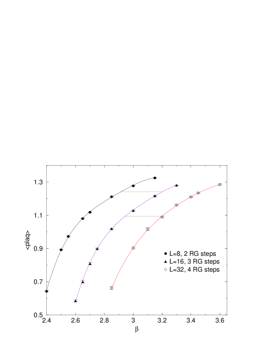
Figure 5: This figure offers a graphical way to determine the shift $\triangle\beta$ as the function of $\beta$. The change of scale between $\tilde{\beta}=\beta-\triangle\beta(\beta)$ and $\beta$ is a factor of 2: $a(\tilde{\beta})=2a(\beta)$. The length of the horizontal line between the $L=16$ and $L=8$ curves gives the estimate $\triangle\beta(\beta=3.20)=0.285$ (3 vs. 2 blocking steps), that of between $L=32$ and $L=16$ leads to $\triangle\beta(\beta=3.20)=0.257$ (4 vs. 3 blocking steps).

We made a standard two-lattice Monte Carlo renormalization group MCRG analysis in the coupling constant region $\beta\in(2.6-3.5)$ in order to test whether the underlying theory has a single relevant parameter (as a Yang-Mills theory has) and to get quantitative results on the scales, i.e. on $a(\beta)$, where $a$ is the lattice unit. Configurations were generated on $32^{4}$ and $16^{4}$ lattices which were blocked to $2^{4}$ lattices using 4 and 3 RG steps, respectively. A simple Swendsen-type blocking [15] was used and the block average was projected back to the discrete subgroup after every block step. On the $2^{4}$ blocked configurations the plaquette and the length-6 twisted loop were measured. They correspond to large smeared loops on the original lattices. Generating the $32^{4}$ configurations at some $\beta$, one is searching for an associated $\tilde{\beta}=\beta-\triangle\beta$ where the $16^{4}$ configurations after 3 blocking steps give the same loop expectation values as the $32^{4}$ configurations after 4 steps. The corresponding $\triangle\beta$ ( as the function of $\beta$ ) gives the shift in the coupling which results in a factor of 2 increase in the lattice unit $a$: $a(\tilde{\beta})=2a(\beta)$. In order to see the sensitivity on the number of blocking steps, the procedure was repeated on $16^{4}$ versus $8^{4}$ lattices using 3 and 2 block steps, respectively.

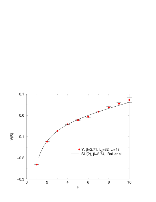
Figure 6: Matching the discrete 120-element $\tilde{Y}$ potential at $\beta_{W}^{120}=2.71$ with that of SU(2) at $\beta_{W}^{\rm SU2}=2.74$ [16]. The scales are related as $a_{\rm SU2}(2.74)/a_{\tilde{Y}}(2.71)=0.84$.

Fig 5 gives the plaquette expectation values and the figure caption explains how to get the $\triangle\beta$ shifts. The figure for the twisted loop expectation values looks similar. The $\triangle\beta$ shifts from the plaquette and from the twisted loop are consistent indicating that there is one relevant coupling only in this problem. The $\triangle\beta$ values from this analysis (which are not far from the two-loop perturbation theory prediction for SU(2)) suggest that very small lattice units can be obtained in this formulation before approaching the freezing transition at $\beta\sim 6$. On the basis of this RG analysis we estimate that $a(\beta=2.72):a(\beta=2.95):a(\beta=3.20)=4:2:1$. We are not able to give a reliable error estimate here due to the uncontrolled extrapolation errors in the number of blocking steps.

We measured the short distance part of the potential at $\beta=2.71,2.96$ and 3.20 on $32^{3}\times 48,16^{4}$ and $32^{4}$ lattices, respectively, and compared the results with those obtained in SU(2) at $\beta^{\rm SU2}=2.74$ and 2.96 by Bali et al. [16]. After matching the scales and the non-physical constant in the potential the subgroup results are consistent with the SU(2) curve. This is illustrated by Figs. 6 and 7 for $\beta=2.71$ and 3.20, respectively. The quality of the matching is similar at $\beta=2.96$. For the scales in the SU(2) and the subgroup model we obtained $a_{c}(2.74)/a_{d}(2.71)=0.84,a_{c}(2.96)/a_{d}(2.96)=0.86$, and $a_{c}(2.96)/a_{d}(3.20)=1.5$, where ’c’ and ’d’ refer to the continuous and discrete groups, respectively. In Figure 7 the 3 curves with $x=a_{c}(2.96)/a_{d}(3.20)=1.0,1.5,2.0$ illustrate the sensitivity of the matching on $x$. We did not attempt to give errors here since we did not check the finite volume effects and cut-off effects in the short distance part of the potential. In addition, the sensitivity of the matching on the scaling relations is rather weak. From the scale relations above and $a_{c}(2.74)/a_{c}(2.96)=1.86$ [16] one obtains $a_{d}(2.71)/a_{d}(2.96)=1.92$, while the RG analysis gave $a_{d}(2.72)/a_{d}(2.95)=2$. Similarly, one obtains $a_{d}(2.96)/a_{d}(3.20)=1.74$ and $a_{d}(2.95)/a_{d}(3.20)=2$ from potential matching and RG analysis, respectively.

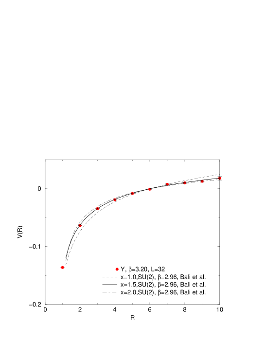
Figure 7: The same as Fig. 6 at $\beta_{W}^{120}=3.20$ and $\beta_{W}^{\rm SU2}=2.96$ [16]. The matching with $x=a_{\rm SU2}(2.96)/a_{\tilde{Y}}(3.20)=1.5$ is close to optimal, while the curves with $x=1.0$ and 2.0 illustrate the (poor) sensitivity of the matching on the ratio of scales.

4 Discussion on the cut-off effects

We want to return to the question of cut-off effects in AF theories. Although there are no rigorous considerations beyond perturbation theory, it is a generally used standard assumption that close to the continuum limit $a^{2}$ powers with logarithms describe the cut-off effects in bosonic theories. Extrapolations of numerical data are done accordingly. The systematic Symanzik improvement program[17] applied in a non-perturbative environment is based on this assumption. We are perplexed by the results in Figure 4 and by the numbers in the $\chi^{2}$ fit. Actually, it has been observed earlier[10] that at $z\gtrsim 5$ a linear fit for $g_{\rm R}$ in $a/L$ was preferred. However, due to larger errors choosing this form was not compelling. The leading order large $N$ result on $g_{R}$ in infinite volume has the expected $\propto a^{2}$ (with logarithms) behavior[11]. It would be interesting to see what happens beyond leading order and in a finite volume. It would be important to check whether other observables, or on-shell quantities like the spectrum show a similar behavior. Obviously, the same questions in d=4 gauge theories are even more relevant.

Acknowledgement

We benefited from numerous discussions with Adrian Patrascioiu and Erhard Seiler on the similarity between the O(3) model and the corresponding discrete models. We are indebted to Andrea Pellisetto and Alan Sokal for sending us the parametrized form of the O(3) finite-size scaling function. We thank Peter Weisz for valuable discussions, in particular for sharing his insight on cut-off effects. We thank also the organizers and participants of the exciting and enjoyable Ringberg Workshop (April 2000), where we had the possibility to present some the results of this paper. We are also indebted to David Kaplan, Julius Kuti and Zoltán Rácz for useful correspondence.

References

- [1] C. Rebbi, Phys. Rev. D21 (1980) 3350; G. Bhanot and C. Rebbi, Phys. Rev. D24 (1981) 3319.
- [2] J. V. José, L. P. Kadanoff, S. Kirkpatrick and D. R. Nelson, Phys. Rev. B16 (1977) 1217; J. Fröhlich and T. Spencer, Comm. Math. Phys. 81 (1981) 527.
- [3] A. Patrascioiu and E. Seiler, Phys. Lett. B430 (1998) 314; ibid B445 (1998) 160; hep-lat/0002012.
- [4] W. M. Fairbain, T. Fulton, and W. H. Klink, J. Math, Phys. 5 (1964) 1038.
- [5] D. Kaplan, private communication.
-
[6]
M. N. Barber, in Phase transitions and critical phenomena, vol.8,
ed. C. Domb and J. L. Lebowitz (Academic Press, London, 1983);
J. L. Cardy, ed., Finite-size scaling (North-Holland, Amsterdam, 1988). - [7] M. Lüscher, P. Weisz and U. Wolff , Nucl. Phys. B359 (1991) 221.
- [8] S. Carracciolo, R. G. Edwards, S. J. Ferreira, A. Pelissetto, and A. D. Sokal, Phys. Rev. Let. 74 (1995) 2969.
- [9] J. Salas and A. D. Sokal, J. Statist. Phys. 88 (1997) 567.
- [10] J. Balog, M. Niedermaier, F. Niedermayer, A. Patrascioiu, E. Seiler and P. Weisz, Phys. Rev. D60 (1999) 094508.
- [11] M. Campostrini, A. Pelissetto, P. Rossi, and E. Vicari, Nucl. Phys. B459 (1996) 207.
-
[12]
J. Balog, M. Niedermaier, F. Niedermayer, A. Patrascioiu, E. Seiler
and P. Weisz,
hep-th/0001097;
M. Caselle, M. Hasenbusch, A. Pelissetto, and E. Vicari, hep-th/0003049. - [13] P. Hasenfratz and F. Niedermayer, Nucl. Phys. B414 (1994) 785.
- [14] F. Niedermayer, Ph. Rüfenacht, U. Wenger, hep-lat/0006xxx.
- [15] R. H. Swendsen, Phys. Rev. Lett. 52 (1984) 2321.
- [16] G. S. Bali, K. Schilling and A. Wachter, Phys. Rev. D55 (1997) 5309.
- [17] K. Symanzik,in New developments in gauge theories, ed. G. ’t Hooft (Plenum, New York, 1980), in Lecture notes in Physics 153, ed. R. Schrader et al. (Springer, Berlin, 1982), in Non-perturbative field theory and QCD, ed. R. Jengo et al. (World Scientific, Singapore, 1983), Nucl. Phys. B226 (1983) 187; 205.