Abstract

We investigate the Abelian monopole condensation in finite temperature SU(2) and SU(3) pure lattice gauge theories. To this end we introduce a gauge invariant disorder parameter built up in terms of the lattice Schrödinger functional. Our numerical results show that the disorder parameter is different from zero and Abelian monopole condense in the confined phase. On the other hand our numerical data suggest that the disorder parameter tends to zero, in the thermodynamic limit, when the gauge coupling constant approaches the critical deconfinement value. In the case of SU(3) we also compare the different kinds of Abelian monopoles which can be defined according to the choice of the Abelian subgroups.

PACS number(s): 11.15.Ha

I. INTRODUCTION

The dual superconductivity of the vacuum in gauge theories to explain color confinement has been proposed since long time by G. ’t Hooft [1] and S. Mandelstam [2]. These authors proposed that the confining vacuum behaves as a coherent state of color magnetic monopoles. In other words the confining vacuum is a magnetic (dual) superconductor. This fascinating proposal offers a picture of confinement whose physics can be clearly extracted. Indeed, the dual Meissner effect causes the formation of chromoelectric flux tubes between chromoelectric charges leading to a linear confining potential.

Following Ref. [3] let us consider gauge theories without matter fields. In order to realize gauge field configurations which describe magnetic monopoles we need a scalar Higgs field [4]. In the ’t Hooft’s scheme the role of the scalar field is played by any operator which transforms in the adjoint representation of the gauge group. Let $X(x)$ be an operator in the adjoint representation, then one fixes the gauge by diagonalizing $X(x)$ at each point. This choice does not fix completely the gauge, for it leaves as residual invariance group the maximal Abelian (Cartan) subgroup of the gauge group. This procedure is known as Abelian projection [3]. The world line of the monopoles can be identified as the lines where two eigenvalues of the operator $X(x)$ are equal. Thus, the dual superconductor idea is realized if these Abelian monopole condense. Due to the gauge invariance we expect that the monopole condensation should manifest irrespective to the gauge fixing. In other words all the Abelian projections are physically equivalent. However, it is conceivable that the dual superconductor scenario could manifest clearly with a clever choice of the operator $X(x)$. It is remarkable that, if one adopts the so called maximally Abelian projection [5], then it seems that the Abelian projected links retain the information relevant to the confinement [6].

It turns out that the Abelian projection can be implemented on the lattice [5], so that one can analyze the dynamics of the Abelian projected gauge fields by means of non perturbative numerical simulations. Indeed, the first direct evidence of the dual Abrikosov vortex joining two static quark-antiquark pair has been obtained in lattice simulations of gauge theories [6, 7, 8, 9]. In particular in Ref. [8] we considered the pure gauge $SU(2)$ lattice theory and found evidence of the dual Meissner effect both in the maximally Abelian gauge and without gauge fixing. Moreover we showed that the London penetration length is a physical gauge invariant quantity.

An alternative and more direct method to detect the dual superconductivity relies upon the very general assumption that the dual superconductivity of the ground state is realized if there is condensation of Abelian monopoles. Thus, according to Ref. [10] it suffices to measure a disorder parameter defined as the vacuum expectation value of a nonlocal operator with non zero magnetic charge and non vanishing vacuum expectation value in the confined phase. However, in the case of non Abelian gauge theories, the disorder parameter is expected to break a non Abelian symmetry, while the dual superconductivity is realized by condensation of Abelian monopoles. As we have already argued, the Abelian monopole charge can be associated to each operator in the adjoint representation by the so-called Abelian projection [3, 5]. Indeed, the authors of Ref. [10] introduced on the lattice a disorder parameter describing condensation of monopoles within a particular Abelian projection. On the other hand, recent results [11] show that the Abelian monopoles defined through several Abelian projection condense, suggesting that the monopole condensation does not depend on the adjoint operator used in the Abelian projection procedure. This is in accordance with the theoretical expectation that monopole condensation should occur irrespective of the gauge fixing procedure. However, a gauge invariant evidence of the Abelian monopole condensation is still lacking.

The aim of the present paper is to investigate the Abelian monopole condensation in pure lattice gauge SU(2) and SU(3) theories in a gauge-invariant way [12]. To do this we introduce a disorder parameter defined in terms of a gauge-invariant thermal partition functional in presence of an external background field.
The plan of the paper is as follows. In Section II we introduce the thermal partition functional, built up using the lattice Schrödinger functional [13, 14]. In Section III we study the Abelian monopole condensation for finite temperature SU(2) lattice gauge theory. Section IV is devoted to the case of SU(3) gauge theory at finite temperature, where, according to the choice of the Abelian subgroup, different kinds of Abelian monopoles can be defined. Our conclusions are drawn in Section V.

II. THE THERMAL PARTITION FUNCTIONAL

To investigate the dynamics of the vacuum at zero temperature we introduced [15, 16] the gauge-invariant effective action for external static (i.e. time-independent) background field defined by means of the lattice Schrödinger functional:

$${\mathcal{Z}}[U^{\mathrm{ext}}_{\mu}]=\int{\mathcal{D}}U\;e^{-S_{W}}\,,$$ (2.1)

where $S_{W}$ is the standard Wilson action. The functional integration is extended over links on a lattice with the hypertorus geometry and satisfying the constraints

$$U_{\mu}(x)|_{x_{4}=0}=U^{\mathrm{ext}}_{\mu}(\vec{x})\,.$$ (2.2)

In Equations (2.1) and (2.2) $U^{\mathrm{ext}}_{\mu}(\vec{x})$ is the lattice version of the external continuum gauge field $\vec{A}^{\mathrm{ext}}(\vec{x})=\vec{A}^{\mathrm{ext}}_{a}(\vec{x})\lambda_{a}/2$:

$$U_{\mu}^{\text{ext}}(\vec{x})={\mathrm{P}}\exp\left\{iag\int_{0}^{1}dt\,A^{\text{ext}}_{a,\mu}(\vec{x}+t\hat{\mu})\frac{\lambda_{a}}{2}\right\}\,,$$ (2.3)

where ${\mathrm{P}}$ is the path-ordering operator and $g$ the gauge coupling constant.
The lattice effective action for the external static background field $\vec{A}^{\mathrm{ext}}(\vec{x})$ is given by

$$\Gamma[\vec{A}^{\mathrm{ext}}]=-\frac{1}{L_{4}}\ln\left\{\frac{{\mathcal{Z}}[\vec{A}^{\mathrm{ext}}]}{{\mathcal{Z}}(0)}\right\}\,,$$ (2.4)

where $L_{4}$ is the extension in Euclidean time and $\mathcal{Z}(0)$ is the lattice Schrödinger functional, Eq. (2.1), without the external background field ($U^{\mathrm{ext}}_{\mu}=\mathbf{1}$). It can be shown [15] that in the continuum limit $\Gamma[\vec{A}^{\mathrm{ext}}]$ is the vacuum energy in presence of the background field $\vec{A}^{\mathrm{ext}}(\vec{x})$.

We want now to extend our definition of lattice effective action to gauge systems at finite temperature. In this case the relevant quantity is the thermal partition function. In the continuum we have:

$$\text{Tr}\left[e^{-\beta_{T}H}\right]=\int\mathcal{D}\vec{A}\,\langle\vec{A}\left|e^{-\beta_{T}H}\mathcal{P}\right|\vec{A}\rangle\,,$$ (2.5)

where $\beta_{T}$ is the inverse of the physical temperature, $H$ is the Hamiltonian, and $\mathcal{P}$ projects onto the physical states. As is well known, the thermal partition function can be written as [17]:

$$\text{Tr}\left[e^{-\beta_{T}H}\right]=\int_{A_{\mu}(\beta_{T},\vec{x})=A_{\mu}(0,\vec{x})}\mathcal{D}A_{\mu}(x_{4},\vec{x})\,e^{-\int^{\beta_{T}}_{0}dx_{4}\,\int d^{3}\vec{x}\mathcal{L}_{Y-M}(\vec{x},x_{4})}\,.$$ (2.6)

On the lattice we have:

$$\text{Tr}\left[e^{-\beta_{T}H}\right]=\int_{U_{\mu}(\beta_{T},\vec{x})=U_{\mu}(0,\vec{x})=U_{\mu}(\vec{x})}\mathcal{D}U_{\mu}(x_{4},\vec{x})\,e^{-S_{W}}\,.$$ (2.7)

Comparing Eq. (2.7) with Eqs. (2.1) and (2.2), we get:

$$\text{Tr}\left[e^{-\beta_{T}H}\right]=\int\mathcal{D}U_{\mu}(\vec{x})\,\mathcal{Z}[U_{\mu}(\vec{x})]\,,$$ (2.8)

where $\mathcal{Z}[U_{\mu}(\vec{x})]$ is the Schrödinger functional Eq. (2.1) defined on a lattice with $L_{4}=\beta_{T}$, with “external” links $U_{\mu}(\vec{x})$ at $x_{4}=0$.

We are interested in the thermal partition function in presence of a given static background field $\vec{A}^{\mathrm{ext}}(\vec{x})$. In the continuum this can be obtained by splitting the gauge field into the background field $\vec{A}^{\mathrm{ext}}(\vec{x})$ and the fluctuating fields $\eta(x)$. So that we could write formally for the thermal partition function $\mathcal{Z}_{T}[\vec{A}^{\mathrm{ext}}]$:

$$\mathcal{Z}_{T}[\vec{A}^{\mathrm{ext}}]=\int\mathcal{D}\vec{\eta}\,\langle\vec{A}^{\mathrm{ext}},\vec{\eta}\left|e^{-\beta_{T}H}\mathcal{P}\right|\vec{A}^{\mathrm{ext}},\vec{\eta}\rangle\,.$$ (2.9)

The lattice implementation of Eq. (2.9) can be obtained from Eq. (2.7) if we write

$$U_{k}(\beta_{T},\vec{x})=U_{k}(0,\vec{x})=U^{\text{ext}}_{k}(\vec{x})\widetilde{U}_{k}(\vec{x})\,,$$ (2.10)

where $U^{\text{ext}}_{k}(\vec{x})$ is given by Eq. (2.3) and the $\widetilde{U}_{k}(\vec{x})$’s are the fluctuating links. Thus we get

$$\mathcal{Z}_{T}[\vec{A}^{\mathrm{ext}}]=\int\,\mathcal{D}\widetilde{U}_{k}(\vec{x})\,\mathcal{D}{U}_{4}(\vec{x})\,\mathcal{Z}[U_{k}^{\text{ext}}(\vec{x}),\widetilde{U}_{k}(\vec{x})]\,,$$ (2.11)

where we integrate over the fluctuating links $\widetilde{U}_{k}(\vec{x})$, while the $U_{k}^{\text{ext}}$ links are fixed. Note that in Eq. (2.11) only the spatial links belonging to the hyperplane $x_{4}=0$ are written as the product of the external link $U^{\text{ext}}_{k}(\vec{x})$ and the fluctuating links $\widetilde{U}_{k}(\vec{x})$. The temporal links $U_{4}(x_{4}=0,\vec{x})$ are left freely fluctuating. It follows that the temporal links $U_{4}(x)$ satisfy the usual periodic boundary conditions. We stress that the periodic boundary conditions in the temporal direction are crucial to retain the physical interpretation that the functional $\mathcal{Z}_{T}[\vec{A}^{\text{ext}}]$ is a thermal partition function. In the following the spatial links belonging to the time-slice $x_{4}=0$ will be called “frozen links”, while the remainder will be the “dynamical links”.
From the physical point of view we are considering the gauge system at finite temperature in interaction with a fixed external background field. As a consequence, in the Wilson action $S_{W}$ we keep only the plaquettes built up with the dynamical links or with dynamical and frozen links. With these limitations it is easy to see that in Eq. (2.11) we have

$$\mathcal{Z}\left[U_{k}^{\text{ext}}(\vec{x}),\widetilde{U}_{k}(\vec{x})\right]=\mathcal{Z}\left[U_{k}^{\text{ext}}(\vec{x})\right]\,.$$ (2.12)

Indeed, let us consider an arbitrary frozen link $U^{\text{ext}}_{k}(\vec{x})\widetilde{U}_{k}(\vec{x})$. This link enters in the modified Wilson action by means of the plaquette:

$$P_{k4}(x_{4}=0,\vec{x})=\text{Tr}\left\{U^{\text{ext}}_{k}(\vec{x})\widetilde{U}_{k}(\vec{x})U_{4}(0,\vec{x}+\hat{k})U^{\dagger}_{k}(1,\vec{x})U^{\dagger}_{4}(0,\vec{x})\right\}\,.$$ (2.13)

Now we observe that the link $U_{4}(0,\vec{x}+\hat{k})$ in Eq. (2.13) is a dynamical one, i.e. we are integrating over it. So that, by using the invariance of the Haar measure we obtain

$$P_{k4}(x_{4}=0,\vec{x})=\text{Tr}\left\{U^{\text{ext}}_{k}(\vec{x})U_{4}(0,\vec{x}+\hat{k})U^{\dagger}_{k}(1,\vec{x})U^{\dagger}_{4}(0,\vec{x})\right\}\,.$$ (2.14)

It is evident that Eq. (2.14) in turns implies Eq. (2.12). Then, we see that in Eq. (2.11) the integration over the fluctuating links $\widetilde{U}(\vec{x})$ gives an irrelevant multiplicative constant. So that we have:

$$\mathcal{Z}_{T}\left[\vec{A}^{\text{ext}}\right]=\int_{U_{k}(\beta_{T},\vec{x})=U_{k}(0,\vec{x})=U^{\text{ext}}_{k}(\vec{x})}\mathcal{D}U\,e^{-S_{W}}\,,$$ (2.15)

where the integrations are over the dynamical links with periodic boundary conditions in the time direction. As concerns the boundary conditions at the spatial boundaries, we keep the fixed boundary conditions $U_{k}(\vec{x},x_{4})=U_{k}^{\text{ext}}(\vec{x})$ used in the Schrödinger functional Eq.(2.1). Thus we see that, if we send the physical temperature to zero, then the thermal functional Eq. (2.15) reduces to the zero-temperature Schrödinger functional Eq. (2.1) with the constraints $U_{k}(x)|_{x_{4}=0}=U^{\mathrm{ext}}_{k}(\vec{x})$ instead of Eq. (2.2). In our previous study [15] we checked that in the thermodynamic limit both conditions agree as concerns the zero-temperature effective action Eq. (2.4).

III. ABELIAN MONOPOLE CONDENSATION: SU(2)

Let us consider the SU(2) pure gauge theory at finite temperature. We are interested in the thermal partition function Eq. (2.15) in presence of an Abelian monopole field. In the case of SU(2) gauge theory the maximal Abelian group is an Abelian U(1) group. Thus, in the continuum the Abelian monopole field turns out to be:

$$g\vec{b}^{a}({\vec{x}})=\delta^{a,3}\frac{n_{\mathrm{mon}}}{2}\frac{\vec{x}\times\vec{n}}{|\vec{x}|(|\vec{x}|-\vec{x}\cdot\vec{n})}\,.$$ (3.1)

where $\vec{n}$ is the direction of the Dirac string and, according to the Dirac quantization condition, $n_{\text{mon}}$ is an integer. The lattice links corresponding to the Abelian monopole field Eq. (3.1) can be readily obtained as:

$$U^{\text{ext}}_{k}(\vec{x})=\text{P}\exp\left\{ig\,\int_{0}^{1}dt\,\frac{\sigma_{a}}{2}b^{a}_{k}(\vec{x}+t\hat{x}_{k})\right\}\,,$$ (3.2)

where the $\sigma_{a}$’s are the Pauli matrices. By choosing $\vec{n}=x_{3}$ we get:

$$\begin{split}U^{\text{ext}}_{1,2}(\vec{x})&=\cos[\theta_{1,2}(\vec{x})]+i\sigma_{3}\sin[\theta_{1,2}(\vec{x})]\,,\\ U^{\text{ext}}_{3}(\vec{x})&={\mathbf{1}}\,,\end{split}$$ (3.3)

with

$$\begin{split}\theta_{1}(\vec{x})&=-\frac{n_{\text{mon}}}{4}\frac{(x_{2}-X_{2})}{|\vec{x}_{\text{mon}}|}\frac{1}{|\vec{x}_{\text{mon}}|-(x_{3}-X_{3})}\,,\\ \theta_{2}(\vec{x})&=+\frac{n_{\text{mon}}}{4}\frac{(x_{1}-X_{1})}{|\vec{x}_{\text{mon}}|}\frac{1}{|\vec{x}_{\text{mon}}|-(x_{3}-X_{3})}\,.\end{split}$$ (3.4)

In Equation (3.4) $(X_{1},X_{2},X_{3})$ are the monopole coordinates and $\vec{x}_{\text{mon}}=(\vec{x}-\vec{X})$. In the numerical simulations we put the lattice Dirac monopole at the center of the time slice $x_{4}=0$. To avoid the singularity due to the Dirac string we locate the monopole between two neighboring sites. We have checked that the numerical results are not too sensitive to the precise position of the magnetic monopole.

According to the discussion in the previous Section we are interested in the thermal partition function $\mathcal{Z}_{T}[\vec{A}^{\text{ext}}]$ given by Eq. (2.15). Note that we do not need to fix the gauge due to the gauge invariance of the thermal partition functional against gauge transformations of the external background field. On the lattice the physical temperature $T_{\text{phys}}$ is given by

$$\frac{1}{T_{\text{phys}}}=\beta_{T}=L_{t}\,,$$ (3.5)

where $L_{t}=L_{4}$ is the lattice linear extension in the time direction. In order to approximate the thermodynamic limit the spatial extension $L_{s}$ should satisfy

$$L_{s}\gg L_{t}\,.$$ (3.6)

To this end we performed our numerical simulations on lattices such that

$$\frac{L_{t}}{L_{s}}\leq 4\,.$$ (3.7)

In the numerical simulations we impose periodic boundary conditions in the time direction. As already discussed, at the spatial boundaries the links are fixed according to Eq. (3.3). This last condition corresponds to the requirement that the fluctuations over the background field vanish at infinity.

Following the suggestion of Ref. [11] we introduce the gauge-invariant disorder parameter for confinement

$$\mu=e^{-F_{\text{mon}}/T_{\text{phys}}}=\frac{\mathcal{Z}_{T}[n_{\text{mon}}]}{\mathcal{Z}_{T}[0]}\,,$$ (3.8)

where $\mathcal{Z}_{T}[0]$ is the thermal partition function without monopole field (i.e. with $n_{\text{mon}}=0$).

From Eq. (3.8) it is clear that $F_{\text{mon}}$ is the free energy to create an Abelian monopole. If there is monopole condensation, then $F_{\text{mon}}=0$ and $\mu=1$. To avoid the problem of measuring a partition function we focus on the derivative of the monopole free energy:

$$F^{\prime}_{\text{mon}}=\frac{\partial}{\partial\beta}F_{\text{mon}}\,.$$ (3.9)

It is straightforward to see that $F^{\prime}_{\text{mon}}$ is given by the difference between the average plaquette

$$F^{\prime}_{\text{mon}}=V\left[<P>_{n_{\text{mon}}=0}-<P>_{n_{\text{mon}}\neq 0}\right]\,,$$ (3.10)

where $V$ is the spatial volume.

We use the over-relaxed heat-bath algorithm to update the gauge configurations. Simulations have been performed by means of the APE100/Quadrics computer facility in Bari. Since we are measuring a local quantity such as the plaquette, a low statistics (from 2000 up to 12000 configurations) is required in order to get a good estimation of $F^{\prime}_{\mathrm{mon}}$.

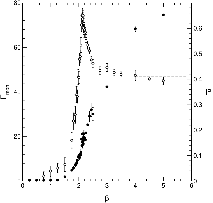
Figure 1: The derivative of the SU(2) monopole free energy versus $\beta$ (Eq. (3.10)) for $n_{\mathrm{mon}}=10$ on a lattice with $L_{t}=4$ and $L_{s}=24$ (open circles), with the absolute value of the Polyakov loop (full circles). The dashed line is Eq. (3.13).

In Figure 1 we display the derivative of the monopole free energy versus $\beta$ for $n_{\text{mon}}=10$ on a lattice with $L_{t}=4$ and $L_{s}=24$. We see that $F^{\prime}_{\text{mon}}$ vanishes at strong coupling and displays a rather sharp peak near $\beta\backsimeq 2.13$. We expect that the peak corresponds to the finite temperature deconfinement transition. In Figure 1 we also display the absolute value of the Polyakov loop:

$$|P|=<|\frac{1}{V}\sum_{\vec{x}}\frac{1}{2}\mathrm{Tr}[\prod_{t=1}^{L_{t}}U_{4}(\vec{x},t)]|>\,,$$ (3.11)

and, indeed, we see that the peak corresponds to the rise of Polyakov loop.
In the weak coupling region the plateau in $F^{\prime}_{\text{mon}}$ indicates that the monopole free energy tends to the classical monopole action which behaves linearly in $\beta$. To see this, we observe that deeply in the weak coupling region the lattice action should reduce to the classical action. In the naive continuum limit the classical action reads :

$$S_{\text{class}}=\;\frac{1}{2}\;\int^{\beta_{T}}_{0}dx_{4}\,\int d^{3}\vec{x}\vec{B}^{a}(\vec{x})\;\vec{B}^{a}(\vec{x})\;$$ (3.12)

where $\vec{B}^{a}(\vec{x})$ is the classical Abelian monopole magnetic field. Introducing an ultraviolet cutoff $\Lambda=\alpha/a$, with $\alpha$ a constant and $a$ the lattice spacing, and performing in Eq. (3.12) the spatial integral over the volume $V=L_{s}^{3}$, we get:

$$S_{\text{class}}\backsimeq\;\frac{\pi\alpha\beta}{8\,T_{\mathrm{phys}}}\;n^{2}_{\text{mon}}+\text{O}(1/L_{s}a)\;.$$ (3.13)

So that in the weak coupling region we have :

$$F^{\prime}_{\mathrm{mon}}\backsimeq\frac{\pi}{8}\alpha n^{2}_{\text{mon}}\;.$$ (3.14)

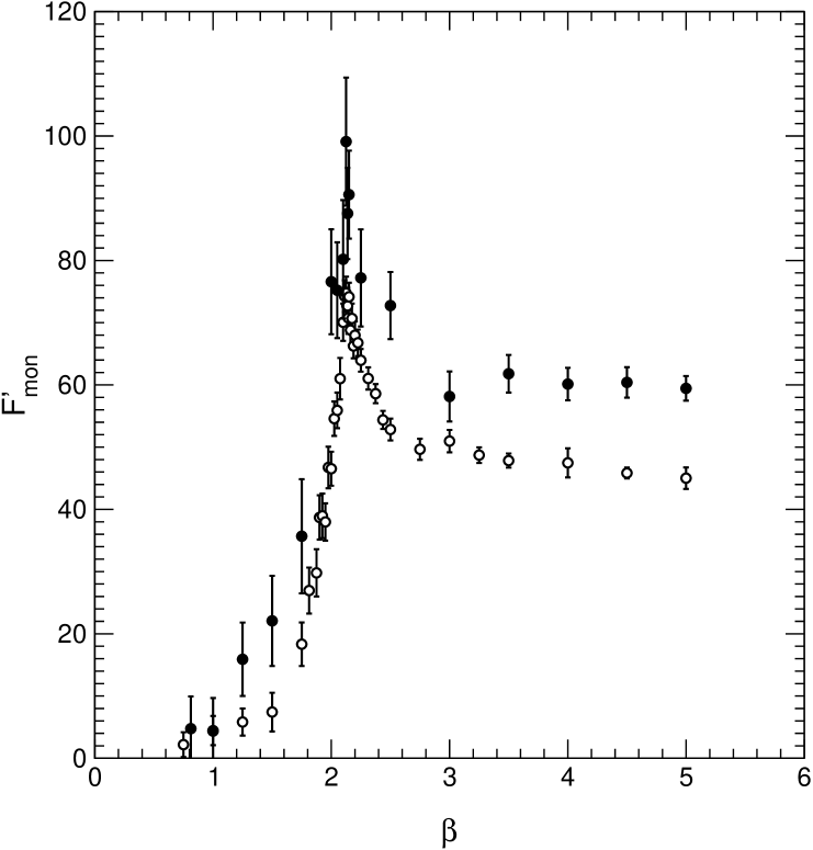
Figure 2: The derivative of the SU(2) monopole free energy versus $\beta$, (Eq. (3.10)), on lattices with $L_{t}=4$ and $L_{s}=24$ (open circles), and $L_{s}=48$ (full circles).

From Figure 1 we see that Eq. (3.14) with $\alpha\backsimeq 1.2$ ( dashed line) describes quite well the numerical data in the relevant region.
In order to determine the critical parameters and the order of the transition, we need to perform the finite size scaling analysis. We plan to do this in a future work. In this paper we restrict ourself to a preliminary qualitative analysis. In Figure 2 we compare the derivative of the monopole free energy on lattices with $L_{t}=4$ and $L_{s}=24,48$. We see that in the strong coupling $F^{\prime}_{\mathrm{mon}}$ agrees for the two lattices. On the other hand, in the weak coupling region the different values of the plateaus can be ascribed to finite volume effects. In the critical region we see that the peak increases.

With the aim of obtaining the disorder parameter $\mu$ (Eq. (3.8)) we perform the numerical integration of the monopole free energy derivative

$$F_{\text{mon}}(\beta)=\int_{0}^{\beta}d\beta^{\prime}\,F^{\prime}_{\text{mon}}(\beta^{\prime})\,.$$ (3.15)

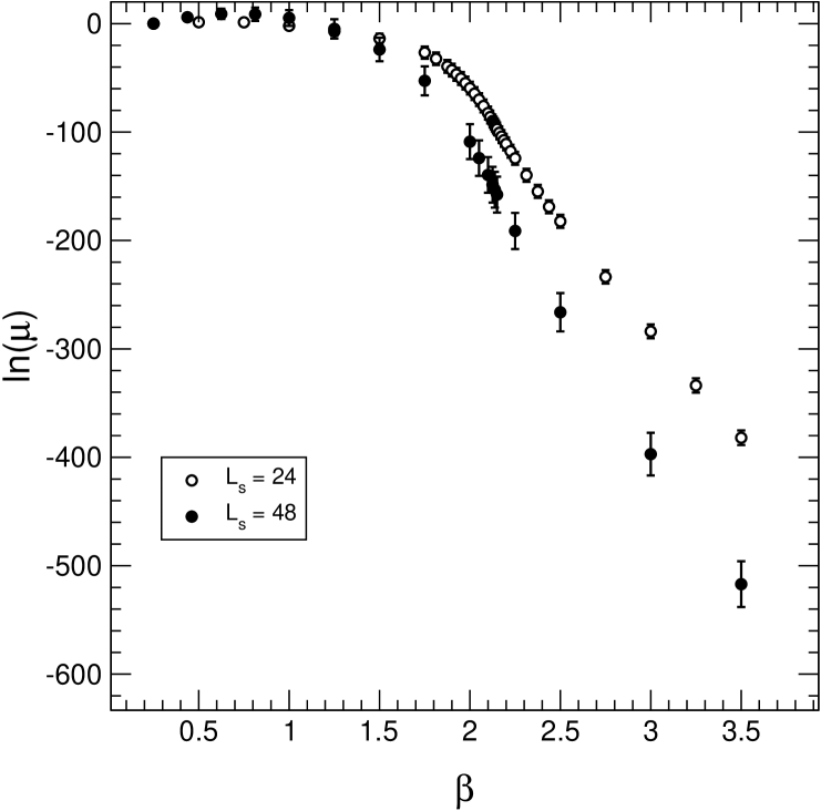
Figure 3: The disorder parameter $\mu$ (Eq. (3.8)) for the SU(2) monopoles versus $\beta$ for lattices with $L_{t}=4$ and $L_{s}=24$ (open circles), or $L_{s}=48$ (full circles).

In Figure 3 we show the disorder parameter $\mu$ versus $\beta$ for lattices with $L_{t}=4$ and $L_{s}=24,48$. We see clearly that $\mu=1$ in the confined phase. In other words the monopoles condense in the vacuum. On the other hand, it seems that $\mu\to 0$ in the thermodynamic limit when $\beta$ reaches the critical value . Indeed, by increasing the spatial volume of the lattice, the disorder parameter $\mu$ decreases faster toward zero. Moreover we see that the finite volume behavior of our disorder parameter is consistent with a second order deconfinement phase transition.
It worthwhile to comment on the finite volume effects. As a matter of fact, it appears that, even though the spatial volume of our larger lattice looks enormous, we gain a rather small increase in the peak value of the monopole free energy derivative. This can be understood by observing that, due to our peculiar conditions at the spatial boundaries, the dynamical volume is smaller than the geometrical one. Moreover, it is well known that the fixed boundary conditions for the gauge fields lead to more severe finite volume effects with respect to the usual periodic boundary conditions. So that, to reach the thermodynamic limit we must simulate our gauge system on lattices with very large spatial volumes. We stress again that the precise determination of the critical parameters requires a finite size scaling which will be presented elsewhere.

IV. ABELIAN MONOPOLE CONDENSATION: SU(3)

In the case of SU(3) gauge theory, the maximal Abelian group is U(1)$\times$U(1). Therefore we have two different types of Abelian monopole. Let us consider, firstly, the Abelian monopole field given by Eq. (3.1), which we call the $T_{3}$ Abelian monopole. The lattice links are given by

$$U_{1,2}^{\text{ext}}(\vec{x})=\begin{bmatrix}e^{i\theta_{1,2}(\vec{x})}&0&0\\ 0&e^{-i\theta_{1,2}(\vec{x})}&0\\ 0&0&1\end{bmatrix}\,,$$ (4.1)

with $\theta_{1,2}(\vec{x})$ defined in Eq. (3.4). The second type of independent Abelian monopole can be obtained by considering the diagonal generator $T_{8}$. In this case we have the $T_{8}$ Abelian monopole:

$$U_{1,2}^{\text{ext}}(\vec{x})=\begin{bmatrix}e^{i\theta_{1,2}(\vec{x})}&0&0\\ 0&e^{i\theta_{1,2}(\vec{x})}&0\\ 0&0&e^{-2i\theta_{1,2}(\vec{x})}\end{bmatrix}\,,$$ (4.2)

with

$$\begin{split}\theta_{1}(\vec{x})&=\frac{1}{\sqrt{3}}\left[-\frac{n_{\text{mon}}}{4}\frac{(x_{2}-X_{2})}{|\vec{x}_{\text{mon}}|}\frac{1}{|\vec{x}_{\text{mon}}|-(x_{3}-X_{3})}\right]\,,\\ \theta_{2}(\vec{x})&=\frac{1}{\sqrt{3}}\left[+\frac{n_{\text{mon}}}{4}\frac{(x_{1}-X_{1})}{|\vec{x}_{\text{mon}}|}\frac{1}{|\vec{x}_{\text{mon}}|-(x_{3}-X_{3})}\right]\,.\end{split}$$ (4.3)

Obviously, the lattice links Eq. (4.2) corresponds now to the continuum gauge field

$$g\vec{b}^{a}({\vec{x}})=\delta^{a,8}\frac{n_{\mathrm{mon}}}{2}\frac{\vec{x}\times\vec{n}}{|\vec{x}|(|\vec{x}|-\vec{x}\cdot\vec{n})}\,.$$ (4.4)

The other Abelian monopoles can be generated by considering the linear combination of the $T_{3}$ and $T_{8}$ generators. In particular we have considered the $T_{3a}$ Abelian monopole corresponding to the following linear combination [11] of $\lambda_{3}/2$ and $\lambda_{8}/2$:

$$T_{3a}=-\frac{1}{2}\frac{\lambda_{3}}{2}+\frac{\sqrt{3}}{2}\frac{\lambda_{8}}{2}=\begin{bmatrix}0&0&0\\ 0&\frac{1}{2}&0\\ 0&0&-\frac{1}{2}\end{bmatrix}\,.$$ (4.5)

In Figure 4 we compare the free energy monopole derivative for the $T_{3}$, $T_{3a}$ and $T_{8}$ Abelian monopoles for the lattice with $L_{t}=4$ and $L_{s}=32$. We see that the $T_{3}$ and $T_{3a}$ Abelian monopoles agree within statistical errors in the whole range of $\beta$. On the other hand the $T_{8}$ Abelian monopole displays a signal about a factor two higher in the peak region. This is at variance of previous studies [11] which find out that the disorder parameters for the three Abelian monopoles defined by means of the Polyakov projection coincide within statistical errors. This result is quite interesting, for it suggests that in the pattern of dynamical symmetry breaking due to the Abelian monopole condensation the color direction $8$ is slightly preferred.
Let us consider, now, in detail the $T_{8}$ Abelian monopole. In Figure 5 we report the derivative of the monopole free energy versus $\beta$ for the lattice with $L_{t}=4$ and $L_{s}=32$. We also display the absolute value of the Polyakov loop:

$$|P|=<|\frac{1}{V}\sum_{\vec{x}}\frac{1}{3}\mathrm{Tr}[\prod_{t=1}^{L_{t}}U_{4}(\vec{x},t)]|>\,,$$ (4.6)

We see that $F^{\prime}_{\text{mon}}$ behaves like in the SU(2) case. Indeed, the free energy monopole derivative is zero within errors in the strong coupling region, while it display a sharp peak in correspondence of the rise of the Polyakov loop. In the weak coupling region $F^{\prime}_{\text{mon}}$ is almost constant. The value of the plateau correspond to the classical action Eq. (3.12) which in the present case gives:

$$S_{\text{class}}\backsimeq\;\frac{\alpha\pi\beta}{12\,T_{\mathrm{phys}}}\;n^{2}_{\text{mon}}+\text{O}(1/L_{s}\text{a})\;,$$ (4.7)

so that

$$F^{\prime}_{\mathrm{mon}}=\alpha\frac{\pi}{12}n^{2}_{\mathrm{mon}}\,.$$ (4.8)

The dashed line in Figure 5 in the weak coupling region corresponds to Eq. (4.8) with $\alpha\backsimeq 2.0$.
As in the $SU(2)$ theory we find that by increasing the spatial volume the peak increases (see Figure 6). Our data do not show a measurable shift of the peak. We feel that this is a manifestation of the first order nature of the $SU(3)$ deconfinement transition. This is confirmed if we look at the disorder parameter $\mu$. In Figure 7 we show the disorder parameter $\mu$ versus $\beta$ for the $L_{t}=4$ and $L_{s}=32,48$ lattices. Again we see that the disorder parameter $\mu$ is different from zero in the confined phase and decreases towards zero in the thermodynamic limit when we approach the critical coupling. Moreover our numerical results suggest that by increasing the spatial volume the two curves cross. This is precisely the finite volume behavior expected for the order parameter in the case of a first order phase transition [18].

V. CONCLUSIONS

In this paper we have investigated the Abelian monopole condensation in the finite temperature SU(2) and SU(3) lattice gauge theories. By means of the lattice thermal partition functional we introduce a disorder parameter which signals the Abelian monopole condensation in the confined phase. By construction our definition of the disorder parameter is gauge invariant, so that we do not need to perform the Abelian projection. Our numerical results suggest that the disorder parameter $\mu$ is different from zero in the confined phase and tends to zero when approaching the critical coupling in the thermodynamic limit. We point out that in our approach the precise determination of the critical parameters could be obtained by means of a finite size scaling analysis. However, our results are consistent with a second order deconfining phase transition in the case of the $SU(2)$ gauge theory. On the other hand, in the case of $SU(3)$ the disorder parameter $\mu$ displays the finite-size behavior expected for a first order transition. It is clear that the finite size analysis in the critical region requires a separate study with both better statistic and larger lattice volumes. Remarkably, in the case of SU(3) gauge theory, where there are two independent Abelian monopole fields related to the two diagonal generators of the gauge algebra, we find that the non perturbative vacuum reacts moderately strongly in the case of the $T_{8}$ Abelian monopole. We feel that this last result should be useful in the theoretical efforts to understand the pattern of symmetry breaking in the deconfined phase of QCD.
In conclusion we stress that our approach, while keeping the gauge invariance, can be readily extended to incorporate the dynamical fermions. We hope to present results in this direction in a future study.

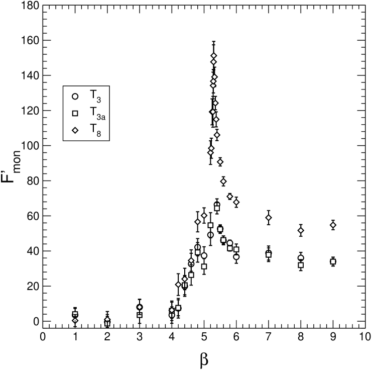
Figure 4: The derivative of the SU(3) monopole free energy in the case of $T_{3}$ (circles), $T_{3a}$ (squares), and $T_{8}$ (diamonds) Abelian monopoles.

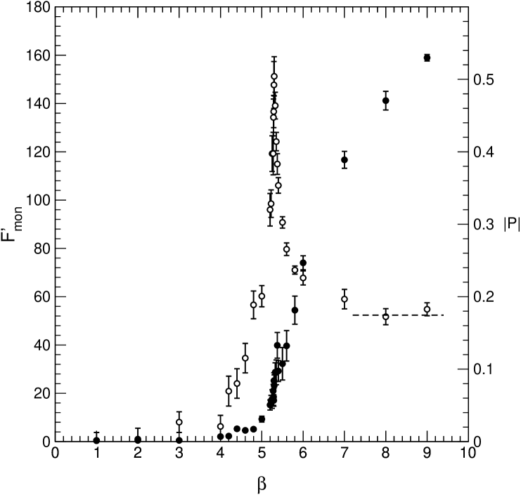
Figure 5: The derivative of the SU(3) monopole free energy for the $T_{8}$ Abelian monopole (open circles) versus $\beta$ with the absolute value of the Polyakov loop (full circles). The dashed line is Eq. (4.8).

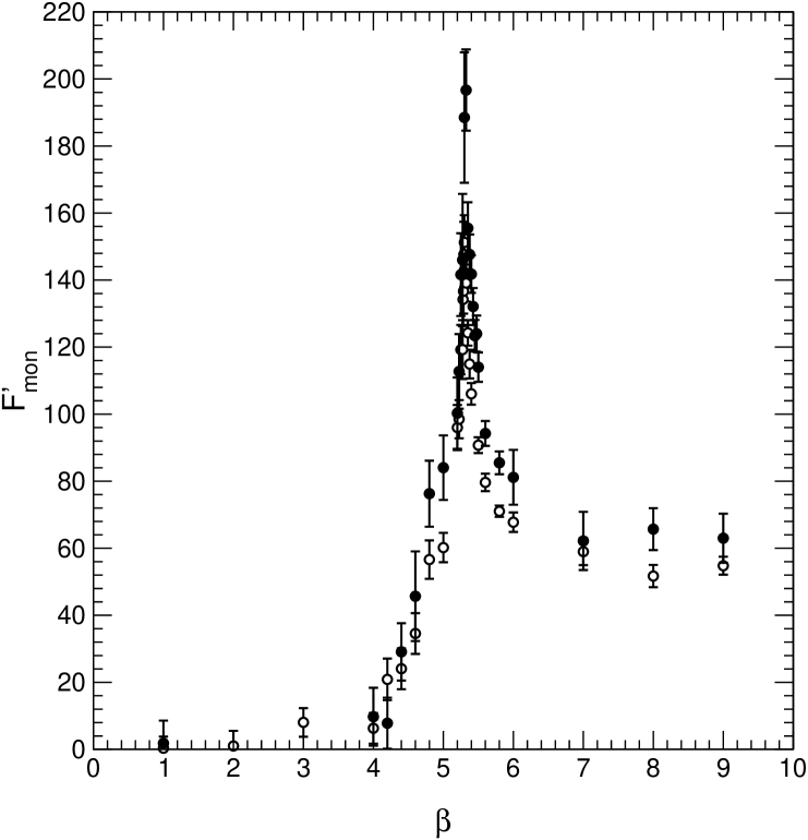
Figure 6: The derivative of the $T_{8}$ Abelian monopole free energy versus $\beta$, on lattices with $L_{t}=4$ and $L_{s}=24$ (open circles), and $L_{s}=48$ (full circles).

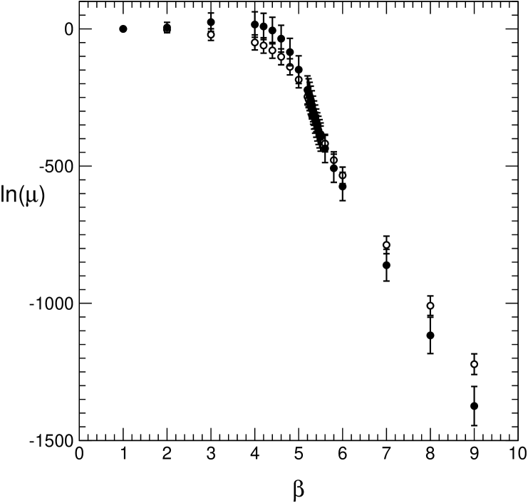
Figure 7: The disorder parameter $\mu$ (Eq. (3.8)) for the SU(3) $T_{8}$ Abelian monopoles versus $\beta$ for lattices with $L_{t}=4$ and $L_{s}=24$ (open circles), and $L_{s}=48$ (full circles).

References

- [1] G. ’t Hooft, in “High Energy Physics”, EPS Int. Conf., Palermo 1975, ed. A. Zichichi.
- [2] S. Mandelstam Phys. Rep. 23C, 245 (1976).
- [3] G. ’t Hooft, Nucl. Phys. B190, 455 (1981); G. ’t Hooft, Physica Scripta 25, 133 (1982).
- [4] A. M. Polyakov, JEPT Lett. 20, 194 (1974); G. ’t Hooft, Nucl. Phys. B79, 276 (1974).
- [5] A. S. Kronfeld, M. L. Laursen, G. Schierholz and U. J. Wiese, Phys. Lett. B198, 516 (1987); A. S. Kronfeld, G. Schierholz and U. J. Wiese, Nucl. Phys. B293, 461 (1987).
- [6] For a review, see: T. Suzuki, Nucl. Phys. Proc. Suppl. 30, 176 (1993); R. W. Haymaker, Phys. Rep. 315, 153 (1999).
- [7] V. Singh, D. A. Browne and R. W. Haymaker, Phys. Lett. B306, 115 (1993).
- [8] P. Cea and L. Cosmai, Nucl. Phys. Proc. Suppl. 30 (1993) 572; Phys. Rev. D52, 5152 (1995).
- [9] G. S. Bali, K. Schilling and C. Schlichter, Phys. Rev. D51, 5165 (1995).
- [10] A. Di Giacomo, Acta Phys. Polon. B25, 215 (1994); L. Del Debbio, A. Di Giacomo and G. Paffuti, Phys. Lett. B349, 513 (1995).
- [11] A. Di Giacomo, B. Lucini, L. Montesi and G. Paffuti, Phys. Rev. D61, 034503 (2000); ibid. D61, 034504 (2000).
- [12] A partial account of the results discussed in the present paper has been reported in P. Cea and L. Cosmai, Nucl. Phys. B (Proc. Suppl.) 83-84 (2000) 428.
- [13] G. C. Rossi and M. Testa, Nucl. Phys. B163, 109 (1980); Nucl. Phys. B176, 477 (1980).
- [14] M. Lüscher, R. Narayanan, P. Weisz and U. Wolff, Nucl. Phys. B384, 168 (1992); M. Lüscher and P. Weisz, Nucl. Phys. B452, 213 (1995).
- [15] P. Cea, L. Cosmai and A. D. Polosa, Phys. Lett. B392, 177 (1997).
- [16] P. Cea and L. Cosmai, Phys. Rev. D60, 094506 (1999)
- [17] D. J. Gross, R. D. Pisarski and L. G. Yaffe, Rev. Mod. Phys. 53, 43 (1981).
- [18] A. Ukawa, Nucl. Phys. Proc. Suppl. 17 (1990) 118 .