DO INSTANTONS OF THE CP(N-1) MODEL MELT?

In the two-dimensional $CP^{N-1}$ model one can parametrize exact many-instanton solutions via $N$ ‘constituents’ (called ‘zindons’). This parameterization allows, in principle, a complete ‘melting’ of individual instantons. The model is therefore well suited to study whether dynamics prefers a dilute or a strongly overlapping ensemble of instantons. We study the statistical mechanics of instantons both analytically and numerically. We find that at $N=2$ the instanton system collapses into zero-size instantons. At $N=3,4$ we find that well-isolated instantons are dynamically preferred though 15-25% of instantons have a considerable overlap with others.

1 Introduction

Instantons, the specific fluctuations of the gluon field, carrying topological charge, play an important role in explaining many features of QCD, like the spontaneous breaking of chiral symmetry $\!{}^{{\bf?},{\bf?}}$. Furthermore, the instanton vacuum calculations are capable of providing the non-perturbative input to a variety of observables in Deep Inelastic Scattering (DIS) like polarized and unpolarized parton distributions $\!{}^{{\bf?}}$, two-hadron distribution amplitudes skewed parton distributions and $\!{}^{{\bf?}}$, higher-twist matrix elements $\!{}^{{\bf?}}$ and other observables.

The role of instantons in the confinement phenomenon is still not clear. In general, a rigorous proof of a linear confining potential between static probe quarks in a 4-dimensional pure Yang–Mills theory from first principles is still missing $\!{}^{{\bf?}}$, while the extraction of that potential from the current lattice data is subject to large systematic uncertainties $\!{}^{{\bf?}}$.

It has been noticed some time ago $\!{}^{{\bf?}}$ that an infinitely rising linear potential may be achieved if the instanton size distribution falls off as $\nu(\rho)\sim 1/\rho^{3}$ at large $\rho$. Such a regime would mean that large instantons overlap, and that the widely used sum ansatz of single instanton solutions is not too meaningful. If instantons are of any relevance for confinement, it cannot be seen in the dilute-gas approximation. Unfortunately, the true multi-instanton solution is not available in QCD: the long-known ADHM multi-instanton solution $\!{}^{{\bf?}}$ is not an explicit one.

This motivates to investigate the overlap of instantons in a theory which is more simple than QCD. Such a theory is the two-dimensional CP^N-1 model. The model contains asymptotic freedom, confinement and instantons whose explicit form is known for any topological number and any number of colors $N$ $\!{}^{{\bf?},{\bf?}}$. The model is solvable at large $N$ $\!{}^{{\bf?},{\bf?}}$ and, most important, the true multi-instanton measure of the theory is known analytically $\!{}^{{\bf?},{\bf?}}$.

This paper reports on some of the results of our study of the statistical mechanics of instantons in the $CP^{N-1}$ model, by combining analytical and numerical methods $\!{}^{{\bf?}}$. Our conclusion is that, though the bulk of instantons appears to be well isolated, some 15-25% of them have a significant overlap.

2 The CP^N-1 model

The CP^N-1 model is defined in two dimensions which can be represented by the complex plain. The dynamical variables are the $N$ complex fields $u_{A},\;A=1,\dots,N$, which are normalized to unity:

$$u_{A}=\frac{v_{A}}{|v|};\quad|v|^{2}=\sum_{A=1}^{N}|v_{A}|^{2}\;.$$ (1)

We shall call the index $A$ ‘color’ in analogy to QCD. From the fields $u_{A}$ a vector potential $A_{\mu}$ can be constructed:

$$A_{\mu}=\frac{i}{2}\left(u_{A}\partial_{\mu}u_{A}^{*}-u_{A}^{*}\partial_{\mu}u_{A}\right),\quad(\mu=1,2)\;.$$ (2)

The theory is defined by the partition function:

$${\cal Z}=\int\!{\cal D}u_{A}(x){\cal D}u^{*}_{A}(x){\cal D}A_{\mu}(x)\delta(|u|^{2}-1)\exp\left(-\frac{1}{g^{2}}\int\!d^{2}x|\nabla_{\mu}u_{A}|^{2}\right),$$ (3)

with the covariant derivative being

$$\nabla_{\mu}=\partial_{\mu}-iA_{\mu}\;.$$ (4)

The fact that the fields $u_{A}$ are normalized to unity makes the theory non-linear. The theory possesses the Abelian gauge invariance. From the vector potential $A_{\mu}$ a topological charge density $q_{T}(x)$ can be defined as:

$$q_{T}(x)=\frac{1}{4\pi}\epsilon_{\mu\nu}F_{\mu\nu}\,,\quad F_{\mu\nu}=\partial_{\mu}A_{\nu}-\partial_{\nu}A_{\mu}\;.$$ (5)

Here $\epsilon_{\mu\nu}$ is the antisymmetric tensor, i.e. $\epsilon_{12}=1,\epsilon_{21}=-1$, and 0 for the other two index combinations. The multi–instanton (multi–anti-instanton) solution of the theory is known exactly $\!{}^{{\bf?},{\bf?}}$ and can be expressed in terms of the unnormalized fields $v_{A}$ up to an inessential constant as a product of simple monomials:

$${\rm\bf instantons}:\quad v_{A} = \prod_{i=1}^{N_{+}}(z-a_{Ai});\quad z=x+iy\;,$$

$${\rm\bf anti-instantons}:\quad v_{A} = \prod_{j=1}^{N_{-}}(z^{*}-b^{*}_{Aj});\quad z^{*}=x-iy\;.$$ (6)

$N_{+}$ is the number of instantons and $N_{-}$ the number of anti-instantons. A single instanton solution is therefore given by a single monomial and characterized by $N$ 2-dimensional points $a_{A}$, which are called ‘instanton zindons’. In the same way the 2-dimensional coordinates $b_{A}$ are called the positions of ‘anti-instanton zindons’. The word zindon is Persian or Tadjik and means ‘prison’ or ‘castle’. There are, thus, $N$ types of ‘colors’ of instanton zindons (denoted by $a_{A}$) and $N$ types of anti-instanton zindons (denoted by $b_{A}$). It is essential, that the true multi-instanton solution is a product and not a sum of single-instanton solutions. As in QCD, single instanton solutions show up as well defined peaks in the topological charge density:

$$v_{A} = (z-a_{A})\;\longrightarrow\;q_{T}(x)=\frac{1}{\pi}\frac{\rho^{2}}{((x-x_{0})^{2}+\rho^{2})^{2}}\;,$$ (7)

where $x_{0}$ is the instanton center coinciding with the center of mass of $N$ zindons of different ‘colors’ and $\rho$, the instanton size, is given by the spatial dispersion of zindons:

$$x_{0} = \frac{1}{N}\sum_{A}a_{A};\quad\ \rho^{2}=\sum_{A}\frac{1}{N}|x_{0}-a_{A}|^{2}\;.$$ (8)

The corresponding single anti-instanton topological charge density has the same form, but with a negative sign, so it forms a local minimum in the topological charge density. For the combination of multi-instantons and multi-anti-instantons one conventionally uses the product ansatz $\!{}^{{\bf?}}$:

$$v_{A}=\prod_{i=1}^{N_{+}}(z-a_{iA})\prod_{j=1}^{N_{-}}(z^{*}-b^{*}_{jA})\;.$$ (9)

Naturally, it is not an exact solution (it becomes such only in the limit of large separations between instanton and anti-instanton zindons), therefore the action computed on this ansatz is not a sum of the individual actions. The corresponding interaction of instantons and anti-instantons formulated in terms of zindons has been found in Ref. $\!{}^{{\bf?}}$, see the factor $w_{ab}$ below. Combining it with the known multi-instanton ($w_{a}$) and multi-anti-instanton ($w_{b}$) weights $\!{}^{{\bf?},{\bf?}}$ describing the interaction of ‘same-kind’ zindons, one writes the partition function in the form of statistical mechanics of interacting particles ($N$ kinds of instanton zindons and $N$ kinds of anti-instanton zindons):

$$Z=\sum_{N_{+}+N_{-}}\frac{e^{i\theta N_{+}}}{(N_{+}!)^{N}}\frac{e^{-i\theta N_{-}}}{(N_{-}!)^{N}}\int{\cal D}a{\cal D}b\Lambda^{2N(N_{+}+N_{-})}w_{a}w_{b}w_{ab}\;.$$ (10)

$\Lambda$ is the only dimensional constant of the theory and can be set to 1. In the parameterization of ref. $\!{}^{{\bf?}}$ $w_{a}$ is given by:

$$w_{a} = \exp\left[\sum_{i<i^{\prime}}^{N_{+}}\sum_{A}\ln((a_{Ai}-a_{Ai^{\prime}})^{2}\Lambda^{2})-\frac{N}{2}\sum_{i,i^{\prime}}^{N}\ln\left[\sum_{A<B}^{N}(a_{Ai}-a_{Bi^{\prime}})^{2}\Lambda^{2}\right]\right]$$ (11)

$$\times\exp\left[N\frac{N_{+}(N_{+}-1)}{2}\ln\frac{N(N-1)}{2}\right]\;.$$

The corresponding weight for the anti-zindon interaction $w_{b}$ is defined similarly. The instanton–anti-instanton interaction is described by the factor $\!{}^{{\bf?}}$:

$$w_{ab} = \exp\left\{2\beta\sum_{i=1}^{N_{+}}\sum_{i^{\prime}=1}^{N_{-}}\sum_{A,B}^{N}{\cal P}_{AB}\ln\left[(a_{Ai}-b_{Bj})^{2}\Lambda^{2}\right]\right\},$$ (15)

$${\cal P}_{AB}=\left\{\begin{array}[]{cc}\frac{N-1}{N};&A=B\\ &\\ -\frac{1}{N};&A\neq B\end{array}\right.\;.$$

$\beta=2\pi/(g^{2}N)$ is the coupling between instantons and anti-instantons. The partition function describes two systems of zindons, namely instanton and anti-instanton ones, experiencing logarithmic interactions, whose strength is $N-1$ times stronger for same-color zindons than for different-color zindons. One has attraction for zindons/anti-zindons of different color and repulsion for zindons/anti-zindons of the same color. At $N=2$ corresponding to the $CP^{1}=O(3)$ model one can think of the ensemble as of that of $e^{+},e^{-},\mu^{+},\mu^{-}$ particles $\!{}^{{\bf?}}$. The interaction of opposite-kind zindons are suppressed by an additional factor $\beta=2\pi/(g^{2}N_{c})$. Since it is a classical system and not a quantum-mechanical one where stable atoms do exist, such an ensemble, i.e. the CP¹ model is unstable, as we will see in the next section.

3 Instanton size distribution

The multi-instanton ansatz (9) allows for a complete ‘melting’ of instantons. Indeed, if zindons $a_{A}$ and $b_{A}$ are evenly distributed in space individual instantons loose any meaning. In principle, another scenario could take place: a clustering of N-plets of zindons of $N$ different ‘colors’ into ‘color-neutral’ objects. If such clusters are well isolated from other color-neutral clusters, they form well-separated or dilute instantons. We recall that a single instanton consists of $N$ zindons $a_{A}$ with different colors $A$. Which scenario takes place in reality is a matter of the dynamics of the ensemble given by the partition function (10).

The partition function (10) describing the instanton–anti-instanton ensemble in the zindon parameterization has been simulated with a Metropolis algorithm in Ref. $\!{}^{{\bf?}}$. One of the main objectives has been to find the size distribution of instantons.

The basic question is how to identify instantons and anti-instantons. This is also a serious problem for lattice QCD (see e.g. $\!{}^{{\bf?}}$). In the case of the CP^N-1 model we can compare two ways of extracting the instanton content. The first one, which we call ‘geometrical’, is inspired by the zindon parameterization. Given a configuration of zindons $a_{Ai}$ on the plain being at the thermodynamical equilibrium according to the partition function $Z$ one can group them into instantons using the following procedure:

• Take the group of $N$ zindons of $N$ different colors, which has the smallest dispersion $\rho^{2}=\frac{1}{N}\sum_{A}|a_{A}-x_{0}|^{2}$ out of the ensemble and call this group an instanton of size $\rho$ located at the position $x_{0}=\frac{1}{N}\sum_{A}a_{A}$.

• From the rest of the ensemble take out the next group of $N$ zindons with the smallest dispersion $\rho$, and so on until the whole ensemble has been grouped into instantons (and anti-instantons).

This ‘geometrical’ identification of instantons assumes that the overlap does not affect much the peak structure of the topological charge density.

The second way of looking at the instanton size distribution is through the topological charge density $q_{T}(x)$. To that end we compute $q_{T}$ on a grid from an equilibrium distribution of zindons obtained from running the Metropolis algorithm. The grid size limits the resolution of small size fluctuations, but not of large size ones. The method used to identify instantons is the following:

• Find a local maximum $x_{0}$, i.e. a grid point where the topological charge is larger than the one of the eight surrounding neighbors on the 9-plet centered at this grid point. In the spirit of the single instanton solution take then the first approximation for the instanton size to be $\rho_{0}^{2}=1/(\pi q_{T}(x_{0}))$.

• Interpolate the topological charge density on the 9 plet quadratically and calculate the two curvatures $\lambda_{1}$ and $\lambda_{2}$. If they are both negative then the local maximum is confirmed and we obtain at the same time two further estimates for the density via $\rho_{i}^{2}=\sqrt{4/(\pi|\lambda_{i}|)},\;i=1,2$.

• If all three values $\rho_{0},\rho_{1},\rho_{2}$ are smaller than $L/2$ where $L$ is the size of the box where we place the ensemble, then the local maximum is accepted to be an instanton and the size is given by the geometric mean of all three estimates, i.e. by $\rho=(\rho_{0}\rho_{1}\rho_{2})^{1/3}$.

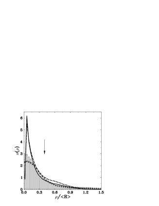
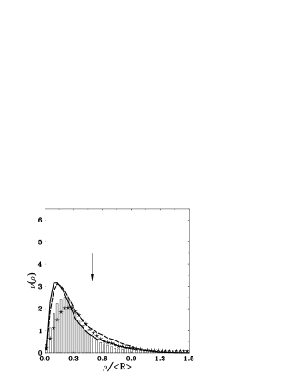
Figure 1: Instanton size distributions are displayed for $N=3$ (left), and $N=4$ (right) for $N_{+}=N_{-}=8$. The histograms show the ‘geometric’ size distributions, and the solid lines the size distributions seen by the ‘lattice’ method, using a $100\times 100$ grid. The instanton–anti-instanton coupling constant for the solid lines and the histograms is $\beta=0$. The stars and the dashed lines show the ‘geometric’ and ‘lattice’ size distributions for the case of $\beta=0.5$. Instanton sizes are plotted in units of the average separation $\langle R\rangle$. The arrows show the maxima of the ‘geometric’ size distributions obtained in the case of purely random space distribution of zindons.

Fig. 1, which has been taken from $\!{}^{{\bf?}}$, shows the size distribution of instantons for $N=3$ and $N=4$. In the case $N=2$ the zindons tend to condense into color neutral pairs and the ensemble collapses, so from that point of view the theory does not exist at all for $N=2$. If one disregards the interaction of instantons with anti-instantons then the attraction of different-color zindons leads to a decrease of the average size of the instantons. This can be seen by comparing the maximum of the size distribution for $\beta=0$ with the maximum for an interaction-less purely random distribution of zindons, which is represented by the arrows.

Switching in instanton–anti-instanton interactions, i.e. moving from $\beta=0$ [histogram/solid line] to $\beta=0.5$ [stars/dashed line] one observes that instantons are on the average shifted to larger sizes, however the effect is rather weak. The effect of the size shrinkage owing to the multi-(anti)instanton weight $w_{a(b)}$ is much more pronounced.

Remarkably, one observes a large discrepancy between the instantons identified by the ‘lattice’ method versus the ‘geometric’ method at small instanton sizes. The discrepancy is prominent at $N=3$ but becomes considerably smaller at $N=4$, so that a tendency is visible that it may die out as $N$ is increased. This phenomenon of unphysical small size fluctuations is similar to the well known ‘dislocation’ phenomenon observed in lattice studies $\!{}^{{\bf?},{\bf?}}$.

For instantons with a size larger than half of the average separation, i.e., $\rho/\langle R\rangle>0.5$ one can say that the overlap becomes essential. This is the case for $15$ – $25\%$ of instantons, displayed in the figure. So one can say that the dilute gas ansatz is justified for many purposes, but that there is a considerable amount of instantons where the overlap cannot be neglected.

4 Summary and conclusions

We have formulated the statistical mechanics of instantons and anti-instantons in the $d=2$ $CP^{N-1}$ model in terms of their ‘constituents’ which we call ‘zindons’. We have derived the interactions of same-kind and opposite-kind zindons for arbitrary $N$.

Though the zindon parameterization of instantons and of their interactions allow for complete ‘melting’ of instantons and is quite opposite in spirit to dilute gas Ansätze, we observe that zindons, nevertheless, tend to form ‘color-neutral’ clusters which can be identified with well-isolated instantons. This effect is due to a combination of two different factors both supporting clustering. One factor is the interactions: same-color zindons are strongly repulsive while different-color zindons are attractive. The second factor is pure geometry: even with a purely random distribution of zindons in space the probability to combine $N$ zindons into a neutral cluster smaller than the average separation is quite sizeable. Both these factors are expected to be even stronger in four dimensions appropriate for the Yang-Mills instantons.

Despite an apparent tendency for clustering of zindons into well-isolated instantons, there always exist a portion of instantons which are strongly overlapping with the others. Depending on what one calls a ‘strong’ overlap we estimate the portion of such instantons to be about 15-25%. If a similar effect takes place in the Yang–Mills case, it means that there are long-range color correlations, which might be relevant to confinement. At the same time if the bulk of instantons are well separated (as we have found for the $CP^{(N-1)}$ model) it would explain the success of instantons in describing physics related to chiral symmetry breaking.

References

References

- [1] D. Diakonov and V. Petrov, Nucl. Phys. B 272, 457 (1986); D. Diakonov, hep-ph/9602375.
- [2] T. Schafer and E. V. Shuryak, Rev. Mod. Phys. 70, 323 (1998) [hep-ph/9610451].
- [3] D. Diakonov, V. Petrov, P. Pobylitsa, M. Polyakov and C. Weiss, Nucl. Phys. B 480, 341 (1996) [hep-ph/9606314]; Phys. Rev. D 56, 4069 (1997) [hep-ph/9703420].
- [4] M. V. Polyakov and C. Weiss, Phys. Rev. D 59, 091502 (1999) [hep-ph/9806390]; ibid. Phys. Rev. D 60, 114017 (1999) [hep-ph/9902451].
- [5] B. Dressler, M. Maul and C. Weiss, Twist-4 contribution to unpolarized structure functions and from instantons, hep-ph/9906444.
- [6] R. W. Haymaker, Phys. Rept. 315, 153 (1999) [hep-lat/9809094].
- [7] D. Diakonov and V. Petrov, Phys. Scripta 61, 536 (2000) [hep-lat/9810037].
- [8] D. Diakonov and V. Petrov, in: Nonperturbative Approaches to QCD, Proc. Internat. workshop at ECT∗, Trento, July 1995, ed. D. Diakonov, PNPI (1995) p. 239.
- [9] M. F. Atiyah, N. J. Hitchin, V. G. Drinfeld and Y. I. Manin, Phys. Lett. A 65, 185 (1978).
- [10] V.L.Golo and A.M.Perelomov, Phys. Lett. B79, 112 (1978).
- [11] A. D’Adda, M. Luscher and P. Di Vecchia, Nucl. Phys. B 146, 63 (1978).
- [12] A. D’Adda, P. Di Vecchia and M. Luscher, Nucl. Phys. B 152, 125 (1979).
- [13] E. Witten, Nucl. Phys. B 149, 285 (1979).
- [14] V. A. Fateev, I. V. Frolov and A. S. Schwarz, Nucl. Phys. B 154, 1 (1979); Sov. J. Nucl. Phys. 30, 590 (1979).
- [15] B. Berg and M. Luscher, Commun. Math. Phys. 69, 57 (1979).
- [16] D. Diakonov and M. Maul, Nucl. Phys. B 571, 91 (2000) [hep-th/9909078].
- [17] A. P. Bukhvostov and L. N. Lipatov, Nucl. Phys. B 180, 116 (1981).
- [18] J. W. Negele, Nucl. Phys. Proc. Suppl. 73, 92 (1999) [hep-lat/9810053].
- [19] B. Berg and M. Luscher, Nucl. Phys. B 190, 412 (1981).
- [20] M. Luscher, Nucl. Phys. B 200, 61 (1982).