Polarized structure functions from the lattice

1 Introduction

Structure functions are an important quantities for understanding hadronic physics from first principles and for confronting experimental measurements. In QCD, the theory of the strong interaction, they probe the underlying make-up of hadrons from the fundamental quarks and gluons. A complete theoretical understanding of hadronic physics requires calculations of these important functions in QCD (or equivalently, a set of operator matrix elements). Because QCD is a confining theory, the complete calculation of the structure functions is necessarily non-perturbative. A rigorous, systematic method for calculating non-perturbatively in QCD is the lattice method, or lattice QCD.

The definition of nucleon structure functions follows from the factorization of the deep inelastic scattering (DIS) cross section of electrons and nucleons.

$$\mathchar 28955\relax_{dis} \sim L_{\mathchar 28950\relax\mathchar 28951\relax}W^{\mathchar 28950\relax\mathchar 28951\relax},$$ (1.1)

$$W^{\mathchar 28950\relax\mathchar 28951\relax} = \frac{1}{4\mathchar 28953\relax}\int{\rm d}^{4}xe^{iq\cdot x}\langle P|[J^{\mathchar 28950\relax}(x),J^{\mathchar 28951\relax}(0)]|P\rangle$$ (1.2)

where $L_{\mathchar 28950\relax\mathchar 28951\relax}$ is the lepton tensor, $W_{\mathchar 28950\relax\mathchar 28951\relax}$ is the hadronic tensor, and $J^{\mathchar 28950\relax}$ is the electromagnetic current. We are interested in the form of $W_{\mathchar 28950\relax\mathchar 28951\relax}$[1].

$$W^{\mathchar 28950\relax\mathchar 28951\relax}(p,q) = \left(-g^{\mathchar 28950\relax\mathchar 28951\relax}+\frac{q^{\mathchar 28950\relax}q^{\mathchar 28951\relax}}{q^{2}}\right)F_{1}(x,Q^{2})$$ (1.3)

$$+ \frac{1}{p\cdot q}\left(p^{\mathchar 28950\relax}-\frac{(p\cdot q)q^{\mathchar 28950\relax}}{q^{2}}\right)\left(p^{\mathchar 28951\relax}-\frac{(p\cdot q)q^{\mathchar 28951\relax}}{q^{2}}\right)F_{2}(x,Q^{2}),$$

where $F_{1}(x,Q^{2})$ and $F_{2}(x,Q^{2})$ are the unpolarized nucleon structure functions. Similarly, for scattering off of polarized nucleons with spin $S$, we have

$$W^{A}_{\mathchar 28950\relax\mathchar 28951\relax}(p,q,S) = i\mathchar 28943\relax_{\mathchar 28950\relax\mathchar 28951\relax\mathchar 28954\relax\mathchar 28955\relax}\frac{Mq^{\mathchar 28954\relax}}{p\cdot q}\left(S^{\mathchar 28955\relax}g_{1}(x,Q^{2})+\left(S^{\mathchar 28955\relax}-\frac{S\cdot q}{p\cdot q}\right)g_{2}(x,Q^{2})\right),$$ (1.4)

where $g_{1}(x,Q^{2})$ and $g_{2}(x,Q^{2})$ are the polarized nucleon structure functions. In the above, $Q^{2}=-q^{2}$ is the momentum transfer from the electron to the struck nucleon, $p^{\mathchar 28950\relax}$ is the incoming nucleon momentum, and $x=Q^{2}/(2p\cdot q)$.

The structure functions $F_{1}$, $F_{2}$, $g_{1}$, and $g_{2}$ are calculable from first principles in QCD. One simply needs to calculate the matrix element in Eq. 1.2.

The nucleon state $|P\rangle$ is a low energy hadronic bound state of quarks and gluons; thus the matrix element, Eq. 1.2, cannot be calculated in perturbation theory. We must use a non-perturbative technique such as the lattice method to calculate it. However, the lattice method works only in Euclidean space-time, while DIS occurs near the light-cone in Minkowski space-time. Thus we cannot calculate the desired matrix element directly. Instead, we resort to the operator product expansion; the non-local operator $[J^{\mathchar 28950\relax}(x),J^{\mathchar 28951\relax}(0)]$ is given in terms of an infinite set of local operators. The utility of the method is that most of these operators are suppressed by powers of $1/Q$. The organization of the expansion is in terms of the so-called twist of the (local) operator, which is defined as the dimension of the operator minus its spin, $T=d-s$. The Wilson coefficients of the expansion, $C_{n}$ are calculable in perturbation theory, and one can show from dimensional reasoning that $C_{n}\sim q^{-(T-2)}$, so at leading order we need only consider $T=2$. We note that the structure functions can be related to $T=2$ distribution functions in the parton picture, i.e., the probability of finding a parton (quark or gluon) with momentum fraction $x$ of the nucleon inside the nucleon. At tree level, the coefficient functions are simply the charges of the partons.

In summary, the calculation of the matrix element is split into two parts, a soft part given by the matrix elements of the local operators, and a hard part given by the $C_{n}$. The dividing line, or scale $\mathchar 28950\relax$, where the split is made is arbitrary. However, at any finite order of perturbation theory, there is residual scheme dependence in $C_{n}$, so one cannot take $\mathchar 28950\relax$ too small. In addition, present lattice simulations have a cut-off $1/a$ around 2-3 GeV. These considerations constrain the range of $\mathchar 28950\relax$ values that can be used.

Looking in more detail, we see that the matrix elements calculated on the lattice are actually moments (in $x$) of the structure functions, or more precisely, their Mellin transforms. Thus in principle, to construct the structure functions one must calculate all of the moments and perform the inverse Mellin transform. Fortunately, for $x$ not very close to 1, we only need the lowest few moments since rapidly, the higher moments begin to probe only the high $x$ region.

The axial and tensor charges are given by the lowest moment of the distribution functions $g_{1}(x)$ and $h_{1}(x)$, the probability of finding a parton with longitudinal or transverse polarization inside a longitudinally or transversely polarized nucleon, respectively.

$$\int{\rm d}x\,g_{1}(x) = \mathchar 28929\relax q,$$ (1.5)

$$2M_{N}S_{\mathchar 28950\relax}\mathchar 28929\relax q = \langle P,S|\bar{q}\mathchar 28941\relax_{\mathchar 28950\relax}\mathchar 28941\relax_{5}q|P,S\rangle,$$ (1.6)

$$\int{\rm d}x\,h_{1}(x) = \mathchar 28942\relax q,$$ (1.7)

$$2(S_{\mathchar 28950\relax}P_{\mathchar 28951\relax}-P_{\mathchar 28950\relax}S_{\mathchar 28951\relax})\mathchar 28942\relax q = \langle P,S|\bar{q}i\mathchar 28955\relax_{\mathchar 28950\relax\mathchar 28951\relax}\mathchar 28941\relax_{5}q|P,S\rangle,$$ (1.8)

where $\mathchar 28929\relax\mathchar 28934\relax=1/2\sum_{q=u,d,s}\mathchar 28929\relax q$ may be interpreted as the quark contribution to the nucleon spin. Also, $\mathchar 28929\relax u-\mathchar 28929\relax d=g_{A}$, the axial coupling. To date, lattice calculations have underestimated the experimental value of the axial charge, $g_{A}=1.26$, by about 20-25%. The tensor charge, which is the lowest moment of the transversity function $h_{1}$[2], is not yet known from experiment, but may soon be measured in polarized Drell-Yan experiments at Brookhaven’s Relativistic Heavy Ion Collider[3]. Theoretical predictions are thus desirable. So far, Kuramashi has given the only estimate[4].

Another detail to note is that lattice and continuum operators are obviously regularized in different schemes, so in any calculation that relies on both regularizations, one must match the two, or require them to be equal, at some renormalization scale, $\mathchar 28950\relax$.

$${\cal O}(\mathchar 28950\relax) = Z_{\cal O}(a\mathchar 28950\relax){\cal O}^{lat}(a)$$ (1.9)

This matching can be done completely in perturbation theory, but it is well known that the bare lattice coupling constant is a poor expansion parameter and lattice perturbation theory is more difficult, besides. An attractive alternative is to use a non-perturbative renormalization (NPR) procedure[5]. The main idea is to mimic a continuum momentum (MOM) scheme on the lattice. Recent calculations show this procedure works quite well[6].

2 Domain wall fermions

A promising new approach for treating fermions on the lattice is domain wall fermions (DWF)[7]. DWF maintain the full chiral symmetry of the continuum at finite lattice spacing. Conventional lattice fermions explicitly break chiral symmetry, an artifact of removing the lattice doublers, which is only restored in the continuum limit. By maintaining this crucial continuum symmetry, simulations with DWF are more continuum-like.

The exact lattice chiral symmetry arises from the addition of an extra, infinite, fifth dimension. The five dimensional fermions have a mass $M(s)$ in the shape of a domain wall ($M(s)<0$ for $s<0$, and $M(s)>0$ for $s>0$ where $s$ is the coordinate in the fifth dimension). Four dimensional chiral zero modes naturally arise on the defect where $M(s)=0$.

The chiral zero modes are four dimensional in the sense that they propagate along the domain wall in ordinary 4d space-time, but not into the fifth dimension. In general they have an exponentially decreasing wave function in the fifth dimension.

For a periodic extra dimension, an anti-domain wall also appears. The chiral zero modes on the anti-domain wall have the opposite handedness as the ones on the domain wall. By coupling both modes to the same 4d gauge field, we can construct a vector gauge theory, for example QCD. When the gauge fields are explicitly four dimensional, one can think of the extra dimension as an internal flavor space. This idea led to the overlap formulation of DWF[8].

As long as the left and right handed zero modes do not overlap in the middle of the fifth dimension, the chiral symmetry is exact. On a finite lattice, however, the tails overlap, and the left and right handed modes mix; an intrinsic quark mass is generated. This quark mass can be made arbitrarily small by increasing the size of the 5th dimension, $N_{s}$ (the number of sites in the fifth dimension).

In practice, we use the boundary fermion variant of DWF[9]. Here, half of the fifth dimension is discarded, so the domain walls become the boundaries of the fifth dimension. An explicit quark mass is introduced by coupling the boundaries with a strength $-m$, i.e., the chiral projections of the five dimensional fields on the boundaries couple to each other with strength $m$, just like a usual fermion mass term. As long the intrinsic mass term is much smaller than $m$, it can be neglected.

It turns out that the exponential rate of damping of the zero mode wave function is controlled by the 5 dimensional quark mass, or domain wall height $M$. Thus, there are three parameters controlling explicit chiral symmetry breaking, $m$, $M$, and $N_{s}$. The formal chiral limit is $N_{s}\to\infty$ and $m\to 0$.

Because they are protected by chiral symmetry, DWF have only ${\cal O}(a^{2})$ errors[10, 11]. This is true at any coupling and in the $N_{s}\to\infty$ limit. At finite $N_{s}$ this is expected to hold up to exponentially small corrections.

In the last section we will see an example of the power of DWF in QCD simulations, the calculation of the negative-parity-nucleon/nucleon mass splitting. This calculation also shows that DWF fermions may be a powerful tool for structure function calculations.

3 Review of lattice results for $g_{A}$.

In this section we briefly review the current results for $g_{A}$ from lattice calculations. This is perhaps the simplest nucleon matrix element one can imagine, and it is troubling that lattice predictions are too low (see table I). Naively, one expects quenching effects to be small since only the valence quarks contribute in the isospin limit. In fact, recent dynamical results also significantly under predict $g_{A}$[12].

Table I: Summary of renormalized results for $g_{{}_{A}}$. Results are for Wilson fermions. In cases where point-split(PS) currents were used, the renormalization was calculated using local currents. While the second entry is consistent with the measured value of $g_{{}_{A}}=1.26$, the configuration ensemble is quite small. Subscript “$\rm con$” refers to the connected contribution to the matrix element.

type of	group	type of	lattice	$\mathchar 28940\relax$	conf.	value
simulation		current	size
Quench	KEK[13]	Local	$16^{3}\times 20$	5.7	260	$g_{{}_{A}}$=0.985(25)
						$\mathchar 28929\relax u_{\rm con}$ = 0.763(35)
						$\mathchar 28929\relax d_{\rm con}$ =-0.226(17)
						$\mathchar 28929\relax\mathchar 28934\relax$ = 0.18(10)
Quench	Liu et al.[14]	Local	$16^{3}\times 24$	6.0	24	$g_{{}_{A}}$=1.18(11)
		PS	$16^{3}\times 24$	6.0	24	$g_{{}_{A}}$=1.20(10)
						$\mathchar 28929\relax u_{\rm con}$= 0.91(12)
						$\mathchar 28929\relax d_{\rm con}$=-0.30(12)
						$\mathchar 28929\relax\mathchar 28934\relax$= 0.25(12)
Quench	DESY[15]	PS	$16^{3}\times 32$	6.0	400-1000	$g_{{}_{A}}$=1.07(9)
						$\mathchar 28929\relax u_{\rm con}$ = 0.830(70)
						$\mathchar 28929\relax d_{\rm con}$ =-0.244(22)
Full ($n_{f}=2$)	SESAM[12]	Local	$16^{3}\times 32$	5.6	200	$g_{{}_{A}}$=0.907(20)
						$\mathchar 28929\relax u_{\rm con}$ = 0.695(18)
						$\mathchar 28929\relax d_{\rm con}$ =-0.212(8)
						$\mathchar 28929\relax\mathchar 28934\relax$ = 0.20(12)

The problem may be related to the renormalization of the lattice axial current $Z_{A}$, which in general is not equal to one because of explicit chiral symmetry breaking. The values of $g_{{}_{A}}$ in table I were obtained using Wilson fermions and perturbative calculations of $Z_{A}$. These simulations are far from the continuum limit where lattice perturbation theory is trustworthy. There may also be significant discretization errors since each of the studies were done at a single, rather large, lattice spacing.

For DWF, the conserved axial current[16] receives no renormalization. This is not true for the local current. However, recent calculations[6] show that $Z_{A}/Z_{V}=1$, a condition required by the axial Ward-Takahashi identity. Thus, a reliable estimate of $g_{{}_{A}}$ using DWF is given by the ratio of the (unrenormalized) matrix elements $\langle P|A_{\mathchar 28950\relax}|P\rangle/\langle P|V_{\mathchar 28950\relax}|P\rangle$ since $\langle P|V_{\mathchar 28950\relax}|P\rangle=1$ in the continuum.

4 Nucleon spectrum using domain wall fermions

In Fig. 1 we show the low energy nucleon spectrum as a function of the quark mass, $m$[17]. The data are all for $6/g^{2}=6.0$ (quenched), $M=1.8$, and lattice size $16^{3}\times 32\times 16$. We use 205 gauge configurations for the lightest two quark masses, $m=0.02$ and 0.03 and 24 configurations for the heavier ones, $m=0.04\to 0.125$. For an explanation of the baryon interpolating operators $B^{\pm}_{1,2}$, see Ref. [17]. We omit the point at m=0.02 for the operator $B_{2}^{-}$ since a good plateau in the effective mass plot is absent. The experimental values for $N(939)$, $N^{\prime}(1440)$, and $N^{*}(1535)$ ($m\approx 0$) (bursts) have been converted to lattice units ($a^{-1}\approx 1.9$ GeV from $am_{\mathchar 28954\relax}=0.400(8)$ in the chiral limit) [18].

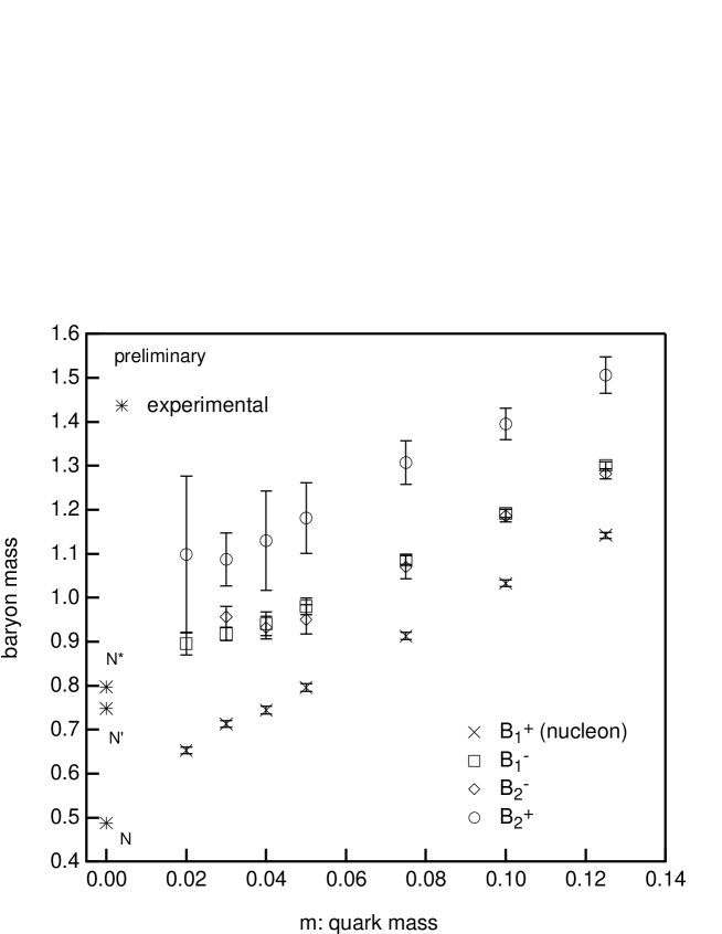
Fig. 1: The low-lying baryon spectrum in lattice units. Note the large mass splitting of $N$ and $N^{*}$ which is within 15% (in the chiral limit) of the experimental value (bursts). The mass of the positive parity excited state is too high, however.

The most remarkable feature in Fig. 1 is the splitting between the nucleon $N$ (from the $B_{1}^{+}$ operator) and its parity partner, $N^{*}$ (from both $B_{1}^{-}$ and $B_{2}^{-}$ operators). In the chiral limit, the mass difference is roughly consistent with experiment (within 15%). To our knowledge, this is the first such demonstration of this important feature of the low-lying nucleon spectrum. Because of the good chiral symmetry of DWF, this result suggests that the mass splitting is due to spontaneous chiral symmetry breaking.

A remaining puzzle is that we cannot extract the nucleon mass from the unconventional nucleon operator $B_{2}^{+}$ which does not have a non-relativistic limit. Instead, $B_{2}^{+}$ gives a signal for the positive parity excited state of the nucleon. To our knowledge, no other groups have succeeded in extracting a clear signal for either the nucleon or its excited state using $B_{2}^{+}$. We suspect that when using DWF the operator $B_{2}^{+}$ has negligible overlap with the nucleon itself, contrary to Wilson quarks where the operators $B_{1}^{+}$ and $B_{2}^{+}$ mix due to explicit chiral symmetry breaking[19]. We confirm such a possibility by comparing the value of the $N^{\prime}$ mass extracted above to the value from a two state fit to the $B_{1}^{+}$ correlation function. Finally, we see no signal for the nucleon state in the mixed correlation function $\langle B_{1}^{+}{\bar{B}}_{2}^{+}+B_{2}^{+}{\bar{B}}_{1}^{+}\rangle$ which leads us to conclude $\langle 0|B_{2}^{+}|N\rangle\simeq 0$.

In Fig. 2 we show the mass ratio of the baryon parity partners ($m_{N^{*}}/m_{N}$) versus the pseudoscalar and vector meson mass ratio ($m_{\mathchar 28953\relax}/m_{\mathchar 28954\relax}$). Experimental points are marked with bursts and correspond to non-strange (left) and strange (right) sectors. In the strange sector we use $\mathchar 28934\relax$ and $\mathchar 28934\relax(1750)$ as the baryon parity partners and $K$ and $K^{*}$ for the mesons. The baryon mass ratio grows with decreasing meson mass ratio. A naive extrapolation is quite consistent with the experimental values. For comparison, we show the recent result of Lee and Leinweber[20] which was obtained using an improved Wilson quark action, D$\mathchar 28959\relax 34$, on coarse lattices.

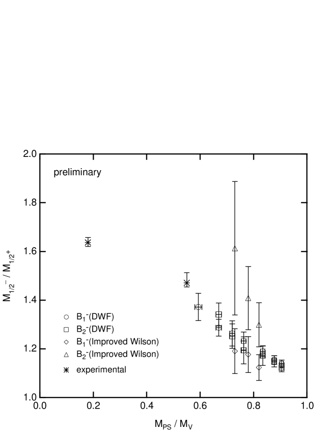
Fig. 2: Mass ratios of the low lying baryon spectrum. Experimental measurements are denoted by bursts. The improved Wilson data (diamonds and triangles) are from Ref.[20].

5 Summary

The DWF results presented here are very encouraging. The negligible mixing between the different operators $B_{1,2}$, and the good agreement with the observed mass splitting of the $N$ and $N^{*}$ states indicate that DWF will work well for the more challenging calculation of nucleon structure functions. The above also confirms our intuition that maintaining chiral symmetry produces more continuum-like lattice simulations. Systematic effects due to finite volume and lattice spacing will be addressed in future calculations. A calculation of nucleon matrix elements using DWF is to be started soon.

References

- [1] See, e.g., R. G. Roberts, “The structure of the proton”, Cambridge University Press (1990).
- [2] R.L. Jaffe, Xiang-dong Ji, Nucl. Phys. B375 (1992), 527
- [3] G. Bunce et al., Particle World 3, 1 (1992); Y. Makdisi, Spin96 Proceedings, ed. C.W. de Jager et al., 107 (1997).
- [4] Y. Kuramashi, Nucl. Phys. A629 (1998), 235c-244c.
- [5] G. Martinelli, et al., Nucl. Phys. B445, 81 (1995).
- [6] See the Lattice ’99 contribution by C. Dawson, hep-lat/9909107. In the case of structure functions, the NPR method has been applied to Wilson quarks which is more problematic due to larger discretization errors and explicit chiral symmetry breaking. See M. Göckeler et al., hep-ph/9909253.
- [7] D. Kaplan, Phys. Lett. B288, 342 (1992).
- [8] R. Narayanan and H. Neuberger, Phys. Lett. B302, 62 (1993); Nucl. Phys. B412, 574(1994).
- [9] Y. Shamir, Nucl. Phys. B409, 90 (1993);
- [10] Y. Kikukawa, R. Narayanan, and H. Neuberger, Phys. Lett. B 399 (1997) 105.
- [11] T. Blum and A. Soni, Phys. Rev. Lett. 79, 3595 (1997); Proceedings of International Europhysics Conference on High-Energy Physics (Jerusalem), 1997, 1034-1038.
- [12] S. Güsken et al., Phys. Rev. D59 (1999), 114502.
- [13] M. Fukugita, Y. Kuramashi, M. Okawa and A. Ukawa, Phys. Rev. Lett. 75 (1995), 2092.
- [14] S.J. Dong, J.-F. Lagaë and K.F. Liu, Phys. Rev. Lett. 75 (1995), 2096; K.F. Liu, S.J. Dong, T. Draper and J.M. Wu, Phys. Rev. D49 (1994), 4755.
- [15] M. Göckeler et al.,Phys. Rev. D53 (1996), 2317.
- [16] V. Furman and Y. Shamir, Nucl. Phys. B439, 54 (1995).
- [17] Some of this data originally appeared in the Lattice ’99 contribution of S. Sasaki, hep-lat/9909093.
- [18] See the Lattice ’99 contributions of L. Wu, hep-lat/9909117, and M. Wingate, hep-lat/9909101.
- [19] D.B. Leinweber, Phys. Rev. D51 (1995), 6383.
- [20] F.X. Lee and D.B. Leinweber, Nucl. Phys. B (Proc. Suppl.) 73 (1999) 258.