UPRF2000-01

SWAT:253

February 2000

Understanding stochastic perturbation theory: toy models and statistical analysis

R. Alfieri $\,{}^{a}$, F. Di Renzo$\,{}^{a}$, E. Onofri$\,{}^{a}$

and

L. Scorzato$\,{}^{a,b}$
${}^{a}\,$Dipartimento di Fisica, Università di Parma

and INFN, Gruppo Collegato di Parma, Parma, Italy
${}^{b}\,$Department of Physics, University of Wales Swansea, UK

Abstract

The numerical stochastic perturbation method based on Parisi–Wu quantisation is applied to a suite of simple models to test its validity at high orders. Large deviations from normal distribution for the basic estimators are systematically found in all cases (“Pepe effect”). As a consequence one should be very careful in estimating statistical errors. We present some results obtained on Weingarten’s “pathological” model where reliable results can be obtained by an application of the bootstrap method. We also present some evidence that in the far less trivial application to Lattice Gauge Theory a similar problem should not arise at moderately high loops (up to $O(\alpha^{10})$).

1. Introduction

In a series of papers [1, 2, 3] it has been shown that the technique of stochastic quantisation introduced by Parisi and Wu [4] can be implemented as a practical algorithm which enables to reach unprecedented high orders in lattice perturbation theory (e.g. $\alpha^{8}$ in the plaquette expectation value in 4-D $SU(3)$ lattice gauge theory). Evaluating perturbative expansion coefficients by a Monte Carlo technique opens the back–door to a number of errors, both statistical and systematic, which should be understood and, hopefully, kept under control. It has been shown in Ref.[5] how systematic errors due to the finite volume can be estimated, putting a limit on the perturbative order reachable on a given lattice size. The aim of the present paper is to present a rather detailed analysis of statistical errors, which present some novel features with respect to the ordinary practice in lattice gauge Monte Carlo. This work was triggered by the observation made by M. Pepe [6] of unexpected large discrepancies with respect to known values in the perturbative coefficients of the non–linear $O(3)\sigma-$model. Starting from this observation (“Pepe effect”) we performed a systematic study of simple models with a small number of degrees of freedom trying to trace the origin of the discrepancies and to resolve them in a reliable way. The crucial fact that our analysis has uncovered is the following: the statistical nature of the processes which enter into the calculation of perturbative coefficients is rapidly deviating from normality as we increase the perturbative order, i.e. the distribution function of a typical coefficient estimator is strongly non–Gaussian, exhibiting a large skewness and a long tail; as a result very rare events give a substantial contribution to the average. A simple minded statistical analysis based on the assumption of normality may grossly fail to identify the confidence intervals; some non–parametric statistical analysis, like the bootstrap method, is necessary to assess the statistical error and provide reliable confidence intervals. This idea will be shown at work in the analysis of a lattice toy model (Weingarten’s “pathological” model [7]) which nevertheless presents many features of interest.

In view of this analysis one should of course worry about the results obtained in Lattice Gauge Theory (LGT). Our main conclusion with this respect is that one is not going to jeopardize the picture we drew in our previous works. As amazing as it can appear at first sight, the application of the method to a by far less trivial model stands on a by far firmer ground. We shall in fact show how the distribution function of coefficient estimators for a typical LGT observable does not exhibit the strongly non–Gaussian nature we find in simpler models.

The content of the paper is organized as follows: in sec.2 we recall the basis facts about Parisi-Wu stochastic technique applied to the numerical calculation of perturbative coefficients in quantum field theory on the lattice (hereafter the “Parisi-WU process” or PW-process for short). In sec.3 we discuss the probability distributions of the PW-process; we shall argue that the customary asymptotic analysis of “sum of identically distributed independent random variables” does not really help at high orders; in this case we shall present numerical evidence showing that the distribution functions still present large deviations from normality, in particular a whole window where the density presents a power–law rather than Gaussian behaviour. We present some detail on the algorithmic implementation of the PW-process in Sec.4 and some numerical results in Sec.5. A discussion of an alternate route is given in Sec.6, based on Girsanov’s formula. We then show (sec.7) how a bootstrap analysis can be very effective in estimating confidence intervals. Finally, in sec. 8, some evidence is produced that both convergence time of the processes and statistical errors are under control for LGT. We present our conclusions in sec. 9. Some details on the bootstrap method and a formal analysis of convergence of perturbative correlation functions are given in appendix.

2. Stochastic perturbation theory

Starting from Parisi and Wu’s pioneering paper, stochastic equations have been used in various forms to investigate quantum field–theoretical models, both perturbatively and non–perturbatively. In particular a Langevin approach can be used as a proposal step subject to a Metropolis check to implement a non–perturbative MonteCarlo for Lattice Gauge Theories. We are concerned here with another approach which makes use of the Langevin equation to calculate weak coupling expansions. The idea [1, 2] is very simple: we start from the Langevin equation (let us focus our attention on a simple scalar field $\varphi$)

(1) $$\frac{\partial\varphi(\boldsymbol{x},t)}{\partial t}=-\frac{\partial S}{\partial\varphi(\boldsymbol{x},t)}+\eta({\boldsymbol{x}},t)$$

where $\eta({\boldsymbol{x}},t)$ is the standard white–noise generalized process; assuming that the action $S$ is splitted into a free $S_{0}$ and an interaction part $g\,S_{1}$, we expand the process $\varphi$ into powers in the coupling constant

(2) $$\varphi({\boldsymbol{x}},t)=\sum_{n=0}^{\infty}g^{n}\,\varphi_{n}({\boldsymbol{x}},t)\;.$$

The Langevin equation is thus translated into a hierarchical system of partial differential equations

(3) $$\frac{\partial\varphi_{0}({\boldsymbol{x}},t)}{\partial t} = -\frac{\partial S_{0}}{\partial\varphi_{0}({\boldsymbol{x}},t)}+\eta(\boldsymbol{x},t)$$

(4) $$\frac{\partial\varphi_{n}({\boldsymbol{x}},t)}{\partial t} = -G_{0}^{-1}\,\varphi_{n}({\boldsymbol{x}},t)+D_{n}(\varphi_{0},\ldots,\varphi_{n-1})\;,\;{\rm for}\;n\geq 1$$

$G_{0}$ being the free propagator and $D_{n}$ representing source terms which can be expressed in terms of higher functional derivatives of the interaction term $S_{1}$. Notice that the source of randomness is confined to the first (free–field) equation; the system can be truncated at any order $n$ due to its peculiar structure ($D_{n}$ depends only on $\varphi_{m}$ with $m<n$).

The system can be used to generate a diagrammatic expansion, as Parisi and Wu did for gauge theories, in terms of the free propagator $G_{0}$; or, it can be studied numerically by simulating the white–noise process, as we have discussed in Ref.[1]. Any given observable ${\mathcal{O}}(\varphi)$ can be expanded in powers of the coupling constant

(5) $${\mathcal{O}}(\varphi)\equiv{\mathcal{O}}\left(\sum_{n\geq 0}g^{n}\,\varphi_{n}\right)=\sum_{n\geq 0}g^{n}\,{\mathcal{O}}_{n}\left(\varphi_{0},\ldots,\varphi_{n}\right)$$

and its expectation value is given by

(6) $$\left\langle{\mathcal{O}}\right\rangle=\left\langle\sum_{n\geq 0}g^{n}\,{\mathcal{O}}_{n}\right\rangle=\sum_{n\geq 0}c_{n}({\mathcal{O}})\,g^{n}\;.$$

The operator ${\mathcal{O}}_{n}$ is therefore an unbiased estimator of the $n-$th expansion coefficient of $\left\langle{\mathcal{O}}\right\rangle$.

It is rather straightforward to implement this idea in a practical algorithm, once the theory has been formulated on a space–time lattice. The application to gauge theory was presented in Ref.[2] using the Langevin algorithm of Batrouni et al. Finite size errors where studied in a subsequent paper [5].

The key problem we want to discuss in the present paper consists in finding a reliable way to estimate the statistical errors in the measure of $\left\langle{\mathcal{O}}_{n}\right\rangle$. Admittedly, it would be desirable to have some analytic information on the nature of the multidimensional coupled stochastic processes  (3). As a substitute we choose to study some toy models where we can perform high statistics calculations and compare the results with the exact coefficients.

3. Toy models.

We have extensively studied the application of numerical stochastic perturbation theory to the following simple models:

1. quartic random variable: $S(\varphi,g)=\mbox{\small$\frac{1}{2}$}\varphi^{2}+\mbox{\small$\frac{1}{4}$}g\varphi^{4}\;,\qquad\varphi\in\mathbb{R}$.

2. dipole random variable: $S(\varphi,g)=[1-\cos(g\,\varphi)]/g^{2},\;\qquad\varphi\in(-\pi,\pi)$.

3. Weingarten’s “pathological model” [7]:

   $$S=\mbox{\small$\frac{1}{2}$}\sum_{\ell}\varphi_{\ell}^{2}+\mbox{\small$\frac{1}{4}$}g\sum_{{\mathfrak{p}}}\,\varphi_{{\mathfrak{p}}}$$

   $$\varphi_{\mathfrak{p}}=\prod_{\ell\in{\mathfrak{p}}}\,\varphi_{\ell}\;,\qquad\varphi_{\ell}\in\mathbb{R},$$

   where $\ell$ runs over links and ${\mathfrak{p}}$ over plaquettes in a simple $n$-dimensional cell of a cubic lattice. We consider $n=2,3,4$.

The integration measure is $\prod d\varphi\exp(-S)$ with the ordinary Lebesgue measure $d\varphi$ over all degrees of freedom; the expectation value of any field observable is then given by

$$\left\langle{\mathcal{O}}\right\rangle=Z^{-1}\int\prod d\varphi\;{\mathcal{O}}[\varphi,g]\,\exp\{-S(\varphi,g)\}\;.$$

The calculation of the weak coupling expansion for the typical observables can be easily performed, except for for the model iii) in four dimensions, where we have been unable to go beyond the $5^{th}$ order. We have for instance for the “quartic” integral

$$\left\langle\varphi^{4}\right\rangle =-\mbox{\small$\frac{1}{4}$}\,\dfrac{d\log(Z(g))}{dg}=1-3\,g-24\,g^{2}-297\,g^{3}-4896\,g^{4}-100278\,g^{4}$$

$$-2450304\,g^{5}-69533397\,g^{6}-2247492096\,g^{7}-81528066378\,g^{8}+O(g^{9})\;,$$

for the “dipole” integral

$$\left\langle\cos(gx)\right\rangle=1-\frac{g^{2}}{2}-\frac{g^{4}}{8}+\frac{17g^{6}}{96}-\frac{29g^{8}}{512}-\frac{251g^{10}}{61440}+O(g^{12})\;,$$

and finally

$$\left\langle\varphi_{\mathfrak{p}}\right\rangle \propto\dfrac{d\log(Z_{3}(g))}{dg}$$

$$=-\frac{g}{4}-\frac{13\,g^{3}}{64}-\frac{103\,g^{5}}{256}-\frac{23797\,g^{7}}{16384}-\frac{2180461\,g^{9}}{262144}-\frac{72763141\,g^{11}}{1048576}-\frac{13342715521\,g^{13}}{16777216}+O(g^{14})\;(n=2)$$

$$=-\frac{g}{4}-\frac{17\,g^{3}}{64}-\frac{595\,g^{5}}{1024}-\frac{34613\,g^{7}}{16384}-\frac{3059191\,g^{9}}{262144}-\frac{388561373\,g^{11}}{4194304}-\frac{67903544647\,g^{13}}{67108864}+O(g^{14})\;(n=3)$$

$$=-\frac{g}{4}-\frac{21\,g^{3}}{64}-\frac{411\,g^{5}}{512}+O(g^{7})\;(n=4)$$

for Weingarten’s model. We have limited ourselves to models involving real random variables which make it very simple to implement the stochastic differential equation Eq.(3). To reach high orders we used a symbolic language to build the right-hand side (i.e. the terms $D_{n}(\varphi_{0},\ldots,\varphi_{n-1})$). In the numerical experiments $n$ is in the range $10$ to $16$.

For the sake of brevity we shall discuss our numerical experiments for the third model, which is the nearest to lattice gauge theory, but the qualitative aspects of the results are indistinguishable in the other models.

Of course one should be aware that Weingarten’s model is rather peculiar; its action is not bounded from below and it may make sense only in Minkowski space. From the perturbative viewpoint, however, it is perfectly admissible and for imaginary $g$ the integrals converge absolutely. So this is an example where perturbation theory for a model living in Minkowski space only can be computed by the stochastic method even if the model does not allow for a Euclidean formulation.

4. Algorithms

Let us describe in some detail the numerical implementation of the stochastic differential equations (3). The free field $\varphi_{0}$ can be computed exactly (as a discrete Markov chain) since it is a Ornstein-Uhlenbeck process [8]. For a time increment $\tau$ we can write

(7) $$\varphi_{0}(t+\tau)=e^{-\tau}\varphi_{0}(t)+\sqrt{1-\exp(-2\tau)}\,N(0,1)$$

where $N(m,\sigma)$ is a normal deviate with mean $m$ and variance $\sigma$. By integrating over the time interval $[t,t+\tau]$ we get

(8) $$\varphi_{n}(t+\Delta t)=e^{-\tau}\varphi_{n}(t)+\int_{t}^{t+\tau}\exp(t^{\prime}-t-\tau)\,D_{n}(\varphi_{0}(t^{\prime}),\ldots,\varphi_{n-1}(t^{\prime}))\,dt^{\prime}$$

which can be approximated, for instance, by the trapezoidal rule. Due to the peculiar nesting of the differential equations it is not necessary to perform the usual “predictor” step to implement the trapezoidal rule, which results in a faster algorithm.

The bias introduced by the approximation is of order $O(\tau^{\nu})$, with $\nu\approx 2$, which should be taken into account as it is usual with the numerical implementation of Langevin equation. In this case however we cannot apply a Metropolis step, as it can be done in the non–perturbative case. The trapezoidal rule and the absence of bias on the free field, however, conspire to keep the finite-$\tau$ error to a small value.

The numerical experiments have been performed by running several independent trajectories in parallel (typically $10^{2}$ to $10^{4}$); a crude estimate of autocorrelation gives a value near to $\tau_{int}=\mbox{\small$\frac{1}{2}$}$ which is the relaxation time of the Ornstein-Uhlenbeck process which drives the whole system. Hence we measure the observable ${\mathcal{O}}_{n}$ every $n_{skip}$ steps with $n_{skip}\,\tau\gtrsim 1$.

The pseudo-random numbers needed to generate the normal deviates are produced through two different algorithms, the lagged–Fibonacci algorithm described by Knuth [9] and Luscher’s algorithm [10]. They do not give appreciably different results in our experiments.

5. Results

We report the results of experiments carried out on the model iii) since it permits a graduation in dimensionality. Other models have been studied in detail and they show the same general pattern. The first three figures are organized as follows: the first plot is a log-log histogram of the raw data for a given observable (i.e. ${\mathcal{O}}_{11}$); the third plot represents $\frac{1}{T}\int_{0}^{T}\left\langle{\mathcal{O}}_{n}\right\rangle\,dt$ averaged over 1000 independent histories. The middle plot represents a blow up of the same average together with some bootstrap sample which allow to estimate confidence intervals, as we describe in some detail later on.

The main observation consists in the fact that the histograms corresponding to high order coefficients deviate substantially from a Gaussian distribution. We do not have a complete characterization of the densities; however the study of these histograms sheds some light on the problem. We observe a rather large window where the densities are dominated by a power–law fall–off. Above a certain order, typically 10-14, the power is approximately $x^{-2-\nu}$ with small $\nu$, which means that there are large deviations from the average which occur as very rare events but contribute to the average. An example is found in Fig. 1 where the time average shows a sharp kink at $t\approx 1.12e4$ and a relaxation thereof. In the first picture the log-log–histogram is contrasted with a $x^{-2}$ and $x^{-3}$ behaviour. Several runs on the same model $iii_{3D})$ are necessary to get a satisfactory estimate of the perturbative coefficient (here $c_{11}=388561373/4194304\approx 92.64$). Another experiment gives more regular histories (see Fig. 2).

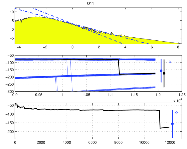
Figure 1. An example of a very rare event in the $O_{11}$ history.

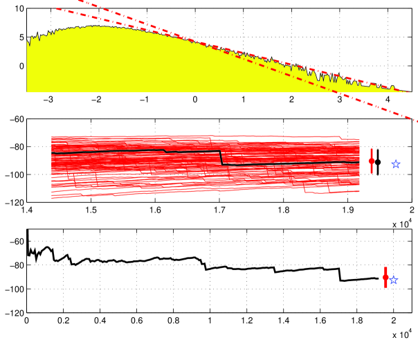
Figure 2. A second $O_{11}$ experiment.

At order 15 we encounter a similar pattern. We observe that the large jumps at $t=1e4$ and $t=1.7e4$ both contribute to reach a value rather close to the exact one. Were it not for the histograms, which, by exhibiting a large $x^{-2-\nu}$ window, warn about very slow convergence, one would be tempted to conclude that a plateau had been reached well before $t\approx 10^{4}$.

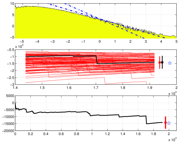
Figure 3. A $O_{15}$ experiment.

On the contrary, low order coefficients are rather close to Gaussian behaviour and the convergence is very fast (see Fig. 4):

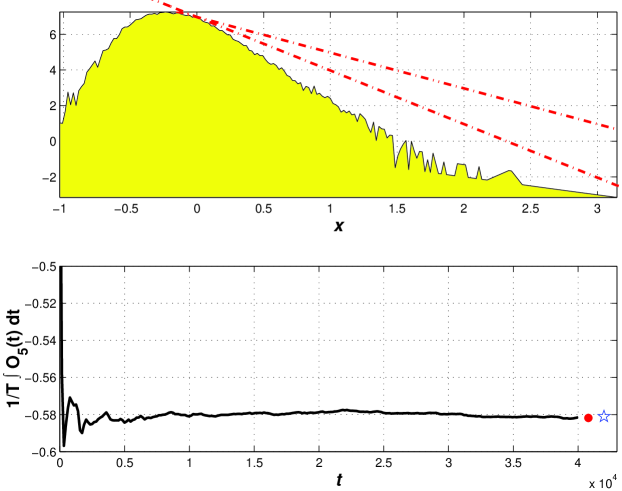
Figure 4. A $O_{5}$ experiment.

We attempted an analytical characterization of the distribution functions $P_{n}({\mathcal{O}}_{n}<x)$ for the processes ${\mathcal{O}}_{n}$. The problem is rather tricky and no explicit formula was reached. One can only show that if ${\mathcal{O}}$ is a generic correlation of fields, and $P_{n}({\mathcal{O}}_{1},\ldots,{\mathcal{O}}_{n},t)$ the distribution function of its first $n$ perturbative coefficients at a Langevin time $t$, then a limit distribution (for $t\rightarrow\infty$) always exists, and that all its moments are finite. In fact this reduces to show that all correlation functions

(9) $$\left\langle\prod_{j}\varphi_{p_{j}}(t)\right\rangle$$

are finite in the limit $t\rightarrow\infty$. Details can be found in App. A.

Since all moments turn out to be finite, one is tempted to use general theorems regarding the sum of independent identically distributed random variables [11]. These could in principle make it unnecessary to have a detailed knowledge of $P_{n}$, since we are averaging over a large number of independent histories and the outcome should be a Gaussian distribution with corrections which can be parameterized and fitted to the data. According to Chebyshev and Petrov

(10) $$\int_{-\infty}^{x}[P^{(k)}_{n}(x)-G(x)]dx=\frac{e^{-x^{2}/2}}{\sqrt{2\pi}}(\frac{Q_{1}^{(k)}(x)}{\sqrt{n}}+\frac{Q_{2}^{(k)}(x)}{n}+\ldots)$$

where the $Q_{i}(x)$ are polynomials, $G(u)$ is the normal distribution and $k$ is the number of independent histories and the convergence is even uniform on $x$. One has for instance

$$Q_{1}^{(k)}(x)=\lambda^{(k)}_{3}\frac{(1-x^{2})}{6};\hskip 28.45274ptQ_{2}^{(k)}(x)=\lambda^{(k)}_{4}x(3-x^{2});$$

$$\lambda^{(k)}_{q}=\frac{\left\langle(\phi^{(k)})^{q}\right\rangle_{c}}{\sigma_{k}^{q}};\hskip 28.45274pt\sigma_{k}^{2}=\left\langle(\phi^{(k)})^{2}\right\rangle.$$

Unfortunately the expansion is, at best, an asymptotic one and no useful estimate on the error was obtained on the basis of these formulas. This fact has triggered our interest on non–parametric methods of analysis which will be presented in sec. 7.

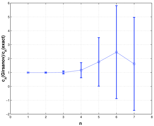
Figure 5. Model $i)$ by Girsanov’s formula.

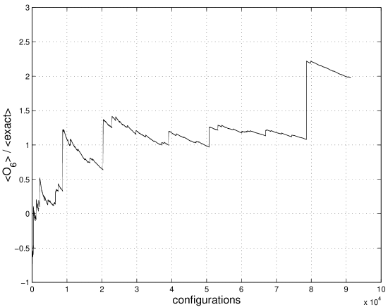
Figure 6. Large deviations in $\left\langle O_{6}\right\rangle$.

6. Girsanov’s formula

The huge jumps in processes ${\mathcal{O}}_{n}$ at high $n$ could in principle be caused by numerical inaccuracy, and for some time we suspected that this could in fact happen. It was soon realized that the large deviations are in fact needed to reach the right average in the long runs, but it was nevertheless reassuring that an alternative method with zero autocorrelation and a totally different algorithm gave the same pattern of configurations. As a matter of fact the method turns out to be less efficient than the direct solution of the system given by Eq.(3), but it is important in order to show that the peculiar properties of the ${\mathcal{O}}_{n}$ histories are not an algorithmic artifact.

The method applies Cameron-Martin-Girsanov formula (see e.g.[12], [13], §3.12)

(11) $$E\Bigl{(}\Phi\bigl{(}\boldsymbol{x}(T)\bigr{)}\;\Big{|}_{w}\Bigr{)}=E\Bigl{(}\Phi\bigl{(}\boldsymbol{y}(T)\bigr{)}\,\exp(\xi_{T})\;\Big{|}_{w}\Bigr{)}$$

where

$$d\boldsymbol{x}(t) = -A\boldsymbol{x}\,dt+\boldsymbol{b}(\boldsymbol{x},t)\,dt+d\boldsymbol{w}(t)$$

$$d\boldsymbol{y}(t) = -A\boldsymbol{y}\,dt+d\boldsymbol{w}(t)\;,\quad(y(0)=x(0))$$

$$\xi(T) = \int_{0}^{T}\boldsymbol{b}(\boldsymbol{y}(\tau),\tau)\cdot d\boldsymbol{w}(\tau)-\mbox{\small$\frac{1}{2}$}\int_{0}^{T}\|\boldsymbol{b}(\boldsymbol{y}(\tau),\tau)\|^{2}\,d\tau$$

and $E\left(.\,|_{w}\right)$ denotes the average with respect to the standard Brownian process $\boldsymbol{w}$. We apply the formula like in Ref.[12], hence $A$ is given by the free inverse propagator and $\boldsymbol{b}(\boldsymbol{x},t)$ is proportional to the coupling constant $g$; therefore we can explicitly expand the “exponential martingale” $\xi(t)$ as a power series in $g$ and get an explicit characterization of the expansion coefficients:

(12) $$\left\langle{\mathcal{O}}_{n}\right\rangle=\lim_{T\to\infty}E\left(H_{n}(I_{1}(T))\;I_{2}^{\frac{n}{2}}(T)/n!\right)$$

where

$$I_{1}(T) = \mbox{\small$\frac{1}{2}$}\int_{0}^{T}\boldsymbol{b}(\boldsymbol{y}(\tau),\tau)\cdot d\boldsymbol{w}(\tau)$$

$$I_{2}(T) = \mbox{\small$\frac{1}{2}$}\int_{0}^{T}\|\boldsymbol{b}(\boldsymbol{y}(\tau),\tau)\|d\tau$$

and $H_{n}$ are Hermite polynomials. This representation of the perturbative coefficients is completely independent on our expansion Eq.(3). It has been implemented as a numerical algorithm and used to estimate the perturbative expansion for model $i)$. Each iteration consists in selecting a normally distributed starting point $x(0)$ and following the evolution up to a time $T$ where transient effects are sufficiently damped; since $A=1$ in our model, $T\geq 1$ is adequate. The samples are statistically independent, modulo the quality of the random number generator. By monitoring the average of $\xi(t)$, which should be exactly one, we have a handle on the accuracy of the algorithm (finite time step and statistics).

The application of Girsanov’s formula gives a cross–check on the existence of large deviations; the algorithm, however, is much more cumbersome to implement on models other than the simple scalar field and even in this latter case it turns out to be less efficient.

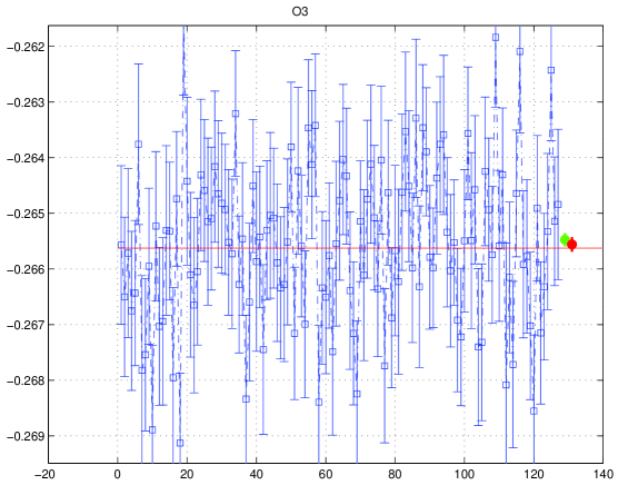
Figure 7. Bootstrap analysis for $O_{3}$.

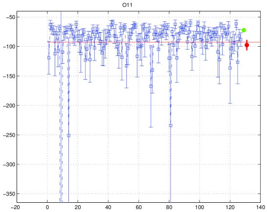
Figure 8. Bootstrap analysis for $O_{11}$.

7. Bootstrap analysis

The consideration of a totally trivial random variable, a high power of a simple normal deviate, is sufficient to convince ourselves that the occurrence of large deviation is actually very natural. Consider a standard Gaussian random variable $x$ and let ${\mathcal{O}}=x^{n}$. The probability density for ${\mathcal{O}}$ contains a power–law prefactor which dominates, for high $n$, over the exponential term. It is clear, by a saddle point argument, that for $n\geq 5$ the average $\left\langle x^{n}\right\rangle$ is dominated by large deviations in the process; this appears to be a common crux in all models we have considered. Having established that the high order coefficients will suffer from large fluctuations, it is important to use reliable tools to estimate the statistical fluctuations. Since our estimators ${\mathcal{O}}_{n}$ will in general have strongly non-Gaussian distribution functions, which moreover are only known empirically through the numerical experiments, it appears a natural choice to apply some non–parametric analysis. We present here the results obtained by applying the bootstrap method [14]. Let us first consider experiments on the 3-D Weingarten’s model, restricted to an elementary cube (a total of 12 link variables, 6 plaquettes). We subdivide the data coming from several runs at the same value $\tau=.01$ (measuring every 100 steps) in bins of $N$ samples (say $N=1000$) and on each bin we perform $B$ bootstrap replicas (in this example $B=100$). Fig.7 reports the result for ${\mathcal{O}}_{3}$. In this case the bootstrap analysis is indistinguishable from a standard gaussian analysis, which means that the distribution is not too far from normal. The standard gaussian analysis is performed by taking a weighted mean of of averages in each sample, i.e.

$$\left\langle X\right\rangle_{gauss} = \dfrac{\sum_{j}\left\langle x_{j}\right\rangle/\sigma_{j}^{2}}{\sum_{j}1/\sigma_{j}^{2}}$$

$$\sigma^{-2} = \sum_{j}\sigma_{j}^{-2}$$

A discrepancy between these values and the bootstrap’s signals a significant deviation from normality, like in Fig.8.

The next plot refers to the estimator ${\mathcal{O}}_{11}$. Here the deviation from normal is relevant: it is clearly reflected in a strong discrepancy between gaussian–like weighted mean and bootstrap estimate. The bootstrap apparently gives a reliable estimate for the confidence interval, as can be seen in the close up picture (Fig. 9).

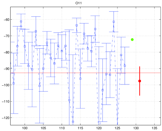
Figure 9. A close up on the previous plot.

Finally let us give a look at the overall pattern obtained in 3-D. Fig. 10 is remarkably similar to the one obtained for the plaquette expansion coefficients in Wilson’s 4-D $SU(3)$ Lattice Gauge Theory.

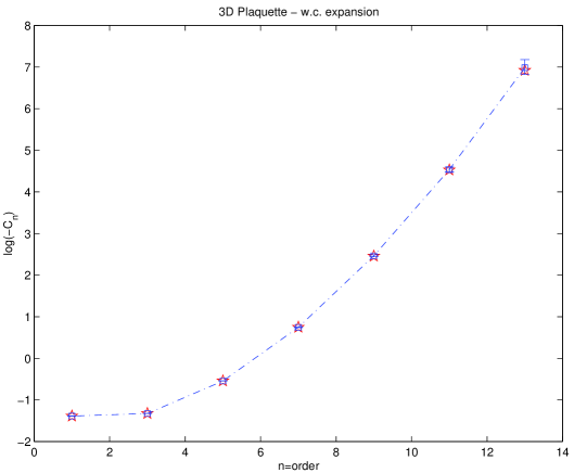
Figure 10. Expansion coefficients for the plaquette variable in 3-D “pathological” model: $\star$=exact, dotted line = MonteCarlo.

8. Lattice Gauge Theories

A good message from this paper is that the picture we just drew for simple models does not spoil the confidence we have in Numerical Stochastic Perturbation Theory for a field of real physical interest like Lattice Gauge Theory. As amazing as it can appear at first sight, this does not totally come as a surprise. In such a theory both the huge number of degrees of freedom and their coupling make it less likely applicable the simple argument of the previous section referring to a high power of a normal variable. One should also keep in mind that the gauge degrees of freedom make it possible to keep the norms of the perturbative components of the field under control by providing a restoring force which does not spoil the convergence of the process.

As hard as formal arguments can be and since an exact characterization of the stochastic processes is missing also for the simple models we considered above, we take a pragmatic attitude. The lesson we can learn from simple models is that monitoring frequencies histograms is a good tool in order to assess huge deviations from normality. By inspecting histograms from Lattice Gauge Theory simulations one can convince oneself that in this case convergence is much more reliable. This of course turns out to be consistent with the bootstrap and standard error analysis giving the same results. For instance, the plot in fig. 11 refers to a $SU(3)$ plaquette high order perturbative coefficient on a small lattice: the process is manifestly safe from “Pepe-effect”.

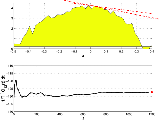
Figure 11. The coefficient of $g^{12}$ for the $SU(3)$ plaquette on a $4^{4}$ lattice.

An independent hint for the reliability of Numerical Stochastic Perturbation Theory for Lattice Gauge Theory comes from [15]. A couple of new perturbative orders in the expansion of the plaquette in 4-D $SU(3)$ (which means reaching $\alpha^{10}$) are shown to be fully consistent with both the expected renormalon behaviour and with finite size effects on top of that. A more organic report on the status of the art concerning the application of the stochastic method to LGT will be given in [16].

9. Conclusions

We have performed a series of simulations to test the numerical stochastic perturbation algorithm previously introduced in the context of Lattice Gauge Theories. The emergence of large non–Gaussian fluctuations in the statistical estimators for high order coefficients was observed in all the simple models we considered with a similar pattern. The study of histograms, giving an estimate of the distribution functions for these estimators, exhibits a large window where exponential fall–off is masked by an approximately power–like behaviour; this fact entails that in any finite run there exist large deviations which are very rare but contribute to the average on the same foot with more frequent events. The lesson we draw from this experiment is twofold: it is necessary to monitor the histograms of the estimators in order to assess the deviation from normality; in case of large deviations, a reliable estimate of statistical error should be obtained by non–parametric methods, such as the bootstrap. These problems do not appear to plague the application of the method to Lattice Gauge Theories. The same viewpoint presented for simple models results in histograms hinting at good convergence properties, fully consistent with all our previous experience in this field.

Appendix A Correlation functions at high Langevin time.

To simplify the argument, let us consider the model $(i)$ with a single degree of freedom (it may be generalized also to realistic systems). First of all we observe that any correlation function of free fields $\varphi_{0}(t)$ may be exactly computed, in fact

(13) $$\left\langle\varphi_{0}(t)^{2m}\right\rangle=(2m-1)!!\,(1-e^{-2t})^{m}$$

converges exponentially to a limit. Then one can proceed by induction: it is sufficient to show that the correlation function Eq.(9), which has a total perturbative order $p_{T}=\sum_{j}p_{j}$, may be written as a finite sum of correlation functions which have a total perturbative order strictly lower than $p_{T}$, plus correlation functions which have a total perturbative order equal to $p_{T}$ but with less free fields, plus exponentially damped terms.

To this end it is useful to re-write the formal solution given by Eq.(8) in discretized time ($t=N\tau$). The idea is to separate the solution into the memory terms, representing the last $N-1$ steps, and the most recent contribution from lower orders and noise.

(14) $$\varphi_{0}(t) = e^{-\tau}\varphi_{0}(t-\tau)+\sqrt{\tau}\eta(t)$$

$$\varphi_{j}(t) = e^{-\tau}\varphi_{j}(t-\tau)+\tau f^{(j)}(t)$$

where

$$f^{(j)}(t)=-\sum_{i=0}^{n-1}\sum_{j=0}^{i}\varphi_{j}(t)\,\varphi_{i-j}(t)\,\varphi_{n-1-i}(t)$$

and $\eta(t)$ are independent gaussian variables with mean zero and variance $2$. We now should put Eq.(14) inside Eq.(9). Let’s do it for a correlation function of two fields (the extension to a general correlation function will be considered later). For any perturbative order $i,j>0$ we have:

$$\left\langle\varphi_{i}(N\tau)\,\varphi_{j}(N\tau)\right\rangle = e^{-2\tau}\left\langle\varphi_{i}(N\tau-\tau)\,\varphi_{j}(N\tau-\tau)\right\rangle+$$

$$+\tau e^{-\tau}\left\langle\varphi_{i}(N\tau-\tau)\,f^{(j)}(N\tau)\right\rangle$$

$$+\tau e^{-\tau}\left\langle\varphi_{j}(N\tau-\tau)\,f^{(i)}(N\tau)\right\rangle$$

$$+\tau^{2}\left\langle f^{(i)}(N\tau)\,f^{(j)}(N\tau)\right\rangle$$

Let us use the general solution of the recursive formula:

$$y_{l}=\alpha_{l}\,y_{l-1}+\beta_{l}$$

which is given by

$$y_{N}=\left(\prod_{m=1}^{N}\alpha_{m}\right)\,y_{0}+\sum_{n=1}^{N}\left(\prod_{m=n+1}^{N}\alpha_{m}\right)\,\beta_{n}$$

In our case we simply have $\alpha_{m}=e^{-2\tau}$, independent on $m$, while $\beta_{m}$ is composed of a linear ($B_{m}$) and a quadratic ($C_{m}$) part in $\tau$:

$$\beta_{m} = \tau\,e^{-\tau}\,B_{m}(\tau)+\tau^{2}\,C_{m}$$

$$B_{m}(\tau) = \left\langle\varphi_{i}(N\tau-\tau)\,f^{(j)}(N\tau)\right\rangle+\left\langle\varphi_{j}(N\tau-\tau)\,f^{(i)}(N\tau)\right\rangle$$

$$C_{m} = \left\langle f^{(i)}(N\tau)\,f^{(j)}(N\tau)\right\rangle.$$

As a result:

$$\left\langle\varphi_{i}(N\tau)\,\varphi_{j}(N\tau)\right\rangle=e^{-2N\tau}\left\langle\varphi_{i}(0)\,\varphi_{j}(0)\right\rangle+$$

$$+ e^{-2N\tau}\left[\sum_{n=1}^{N}e^{2n\tau}(\tau e^{-\tau}B_{n}(\tau)+\tau^{2}C_{n})\right]$$

We observe that $B_{n}(\tau)$ is a correlation function of total perturbative order strictly lower than $i+j$. By inductive hypothesis we know that $B_{n}(\tau)$ has a finite limit for $\tau\rightarrow 0$ (at $t=N\tau$ fixed), let’s say

(17) $$B_{N}(\tau)=B_{t}+O(\tau),$$

and that $B_{t}$ has a finite limit for $t\rightarrow\infty$. Let us parameterize the remaining dependence on $t$ as:

(18) $$B_{t}=B_{\infty}+a_{1}e^{-2t}\,t^{p}+\sum_{q_{j}>2}a_{j}e^{-q_{j}t}$$

From Eq.(13) it follows that the dependence on $t^{p}$ is absent in correlations of free fields, but such correction factors can appear at higher orders. By inserting Eqs.(17,18) in Eq.(A) the geometric series can be re-summed:

$$\left\langle\varphi_{i}(N\tau)\varphi_{j}(N\tau)\right\rangle=e^{-2N\tau}\left\langle\varphi_{i}(0)\varphi_{j}(0)\right\rangle+$$

$$+ e^{-2N\tau}\left[\left(\tau\,B_{t}+O(\tau^{2})\right)\left(\frac{1-e^{2(N+1)\tau}}{1-e^{2\tau}}\right)+O(\tau)\right]$$

If we take first the limit $\tau\rightarrow 0$ at $t=N\tau$ fixed and then $t\rightarrow\infty$, we find

$$\lim_{t\rightarrow\infty}\left\langle\varphi_{i}(t)\varphi_{j}(t)\right\rangle=\tfrac{1}{2}B_{\infty}.$$

Up to now, we have not considered the case of correlation functions with some free fields together with higher order fields. In this case the argument runs almost in the same way, but $\tau f^{(j)}$ is substituted by $\sqrt{\tau}\eta$:

$$\left\langle\varphi_{0}(N\tau)\varphi_{0}(N\tau)(\ldots)\right\rangle = e^{-2\tau}\left\langle\varphi_{0}(N\tau-\tau)\varphi_{0}(N\tau-\tau)(\ldots)\right\rangle+$$

$$+2\sqrt{\tau}e^{-\tau}\left\langle\varphi_{0}(N\tau-\tau)\,\eta(N\tau)\,(\ldots)\right\rangle$$

$$+\tau\left\langle\eta(N\tau)\,\eta(N\tau)\,(\ldots)\right\rangle$$

Only terms with an even number of $\eta$ at time $N\tau$ contributes. In this case the inductive hypothesis must be applied to correlation functions with the same total perturbative order but with a lower number of free fields.

The same argument can be applied to a general correlation function, obtaining in the limit $t\rightarrow\infty$

$$\left\langle\prod_{l=0}^{p}\varphi_{l}^{n_{l}}\right\rangle = \frac{1}{\sum_{l=0}^{p}n_{l}}\left[n_{0}(n_{0}-1)\left\langle\prod_{l=0}^{p}\varphi_{l}^{n_{l}}\,\widehat{(\varphi_{0})^{2}}\right\rangle-\right.$$

$$\left.\sum_{m=1}^{p}n_{m}\sum_{i=0}^{m-1}\sum_{j=0}^{i}\left\langle\prod_{l=0}^{p}\varphi_{l}^{n_{l}}\,\widehat{\varphi_{m}}\,\varphi_{j}\,\varphi_{i-j}\,\varphi_{m-1-i}\right\rangle\right]$$

where $p$ is the maximum perturbative order present, and $\widehat{\varphi}$ means that a factor $\varphi$ should be dropped in the expression.

Induction allows us to conclude that all correlation functions reach a finite limit.

If one goes through the previous argument by keeping the first correction in Eq.(18) it is possible to show that convergence to equilibrium is dominated by an exponential factor which is at least $e^{-2t}$. However, even if in correlations of free fields the dependence on $t$ has exactly an exponential form (or sum of exponentials), in general (at higher orders) one must expect power corrections like $t^{\alpha}\,e^{-2t}$. The precise determination of them is tedious and beyond our scope.

The formula given in Eq.(A) is useful also because it allows to compute not only the mean values of observables but also some high moments of their distributions, at least for the model ($i$). In this way we have been able to show that the large fluctuations were neither an artifact of the numeric simulation nor the effect of a slow convergence to equilibrium.

Appendix B The bootstrap algorithm

The idea of bootstrap is very simple. Let $X$ be a random variable and $x_{1},x_{2},\ldots,x_{N}$ an $N-$tuple of values generated by a physical process, by the stock market, by your Monte Carlo, whichever the case you are currently studying. In the absence of any a priori information on the distribution function for $X$, one makes the most conservative assumption, namely one adopts as distribution function the empirical distribution with density

$$\rho_{boot}^{N}(x)=\frac{1}{N}\sum_{j=1}^{N}\delta(x-x_{j})\;.$$

One then uses $\rho_{boot}$ to generate other $N$-tuples; all values $x_{j}$, $(j=1,\ldots,N)$ being equally probable. Having produced $B$ such $N$-tuples one can estimate various statistics of interest, like mean, median, quartiles etc. For instance the definition of standard deviation is simply

(20) $$\Delta x=\sqrt{\frac{1}{B-1}\sum_{k=1}^{B}\left(\left\langle x\right\rangle_{k}-\left\langle x\right\rangle\right)^{2}}$$

where $\left\langle x\right\rangle_{k}$ is the average computed on the $k$-th $N$-tuple and $\left\langle x\right\rangle$ is their mean value. Recommended values for $B$ are in the range $25\lesssim B\lesssim 200$. It is obvious that no improvement can be obtained on mean values; the virtue of the method should be found in the easy estimation of standard errors which do not rely on the assumption of normality. This does not mean of course that one should not take care of autocorrelation problems or other sources of statistical inaccuracies.

The method is implemented very easily in any language. A one–liner to produce a new $N$-tuple in matlab is the following (if the vector $X$ contains the original data)

XB = X(ceil(N * rand(N,1)));

We refer to Refs.[14, 17] for a thorough discussion of the method.

References

- [1] F. Di Renzo, G. Marchesini, P. Marenzoni, and E. Onofri, Nucl. Phys. B34, 795 (1994).
- [2] F. Di Renzo, G. Marchesini, P. Marenzoni, and E. Onofri, Nucl. Phys. B426, 675 (1994).
- [3] G. Burgio, F. Di Renzo, G. Marchesini, E. Onofri, M. Pepe, and L.Scorzato, Nucl. Phys. B63, 808 (1999).
- [4] G. Parisi and Wu Yongshi, Sci. Sinica 24, 31 (1981).
- [5] G. Marchesini F. Di Renzo and E. Onofri, “Infrared renormalons and finite volume”, Nucl. Phys. B497, 435 (1997).
- [6] M. Pepe, Thesis, University of Milano, 1996.
- [7] D. Weingarten, “Pathological lattice field theory for interacting strings”, Phys. Lett.B 90, 280 (1980).
- [8] G.E. Uhlenbeck and L.S. Ornstein, “On the Theory of Brownian Motion”, Phys. Rev. 36, 823 (1930).
- [9] D.E.Knuth, The Art of Computer Programming, volume 2, Addison Wesley, Reading, Ma., 3rd edition, 1998.
- [10] M. Luscher, “A portable high quality random number generator for lattice field theory simulations”, Comput.Phys.Commun. 79, 100 (1994).
- [11] V.V. Petrov, Limit Theorems of Probability Theory, Number 4 in Oxford studies in probability, Oxford U.P., 1995.
- [12] G. Jona-Lasinio and R. Sénéor, “Study of stochastic differential equations by constructive methods”, J. Stat. Phys., 83(5/6), 1109 (1996).
- [13] I.I. Gihman and A.V. Skorohod, Stochastic Differential Equations, Springer–Verlag, Berlin, 1972.
- [14] B. Efron and R.J. Tibshirani, An Introduction to the Bootstrap, volume 57 of Monographs on Statistics and Applied Probability. Chapman & Hall, N.Y., 1993.
- [15] F. Di Renzo and L. Scorzato, “A consistency check for Renormalons in Lattice Gauge Theory: contributions to the plaquette”, in preparation.
- [16] F. Di Renzo and L. Scorzato, “Understanding Numerical Stochastic Perturbation Theory: a status report for Lattice Gauge Theories”, in preparation.
- [17] A.C. Davison and D.V. Hinkley, Bootstrap Methods and their Applications, Cambridge Series on Statistical and Probabilistic Mathematics. Cambridge University Press, 1997.