Abstract

A numerical study of quenched QCD for light quarks is presented using $O(a)$ improved fermions. Particular attention is paid to the possible existence and determination of quenched chiral logarithms. A ‘safe’ region to use for chiral extrapolations appears to be at and above the strange quark mass.

1 Introduction

The goal of lattice QCD is the computation of physical quantities such as hadron masses and matrix elements using numerical Monte Carlo methods. This has proved to be an ambitious programme because after discretisation of the path integral and generation of a sufficiently large number of independent configurations several limits must be considered:

1. The box size. This is currently at $\sim 1.5-3\,\mbox{fm}$, and should be compared with the nucleon rms radius of $\sim 0.8\,\mbox{fm}$.

2. The chiral limit $m_{q}\to 0$. The $u/d$ and $s$ quarks are light quarks.

3. Continuum limit $a^{k}\to 0$ ($k=2$ if we choose $O(a)$ Symanzik improved fermions, staggered fermions or Ginsparg-Wilson fermions; for Wilson fermions we expect the discretisation effects to have $k=1$).

If all these limits can be successfully taken then presumably QCD will reproduce nature. Although first attempts in this direction are being made, [1], it will require much faster computers to achieve this goal. To reduce the computational effort often the quenched approximation is employed when the fermion determinant is simply set to a constant. However then new problems arise (or are exacerbated):

1. Spurious quenched chiral logarithms appear as $m_{q}\to 0$.

2. The appearance of exceptional configurations.

3. Consistency of the final results when comparing with their experimental or phenomenological values.

In this talk we shall consider points 1 and 2 numerically using $O(a)$ improved fermions.

2 Chiral perturbation theory and quenched chiral logarithms

This was developed by Bernard and Golterman, [2] and Sharpe, [3]. What do we expect? The quenched pseudoscalar effective chiral Lagrangian gives

$$(am_{ps})^{2} \propto (a\widetilde{m}_{q})^{1\over 1+\delta},$$

$$a^{2}g_{P} \equiv \langle 0|\widehat{\cal P}|ps\rangle\propto[(am_{ps})^{2}]^{-\delta},$$

$$am_{ps}af_{ps} \equiv \langle 0|\widehat{\cal A}_{4}|ps\rangle\propto am_{ps}.$$ (1)

As the $\eta^{\prime}$ remains light and has a single and double pole in its propagator, this latter term at $p^{2}=0$, $(m_{0}^{2}/m_{ps}^{2})(1/m_{ps}^{2})$ acts like an extra vertex giving a singular correction to the usually harmless loop term $m_{ps}^{2}\ln(m_{ps}/\Lambda^{2})$ of $m_{0}^{2}\ln(m_{ps}/\Lambda)^{2}$, so that the logarithmic term becomes singular, [4]. This can then be summed to give eq. (1). Normally PCAC, $\partial\cdot{\cal A}=2\widetilde{m}_{q}{\cal P}$, would give us $(am_{ps})^{2}\propto a\widetilde{m}_{q}$. Thus the non-zero $\delta$ leads to singular behaviour for $m_{ps}$ and $g_{P}$ in the chiral limit for quenched QCD. Simple estimates lead to an expectation for $\delta\sim 0.1-0.2$. $\Lambda$ is a cut-off on the $\eta^{\prime}$ loop so $\Lambda\mathrel{\hbox to0.0pt{\lower 4.0pt\hbox{\hskip 1.0pt$\sim$}\hss}\raise 1.0pt\hbox{$<$}}900\,\mbox{MeV}$ and above this scale any singularities are surely damped out. For consistency, we would expect little difference between the PCAC quark mass, $a\widetilde{m}_{q}$, and the ‘standard’ quark mass, $am_{q}\equiv\mbox{\small$\frac{1}{2}$}(1/\kappa-1/\kappa_{c})$.

Similarly by considering the vector/baryon effective chiral Lagrangians, it can be shown that [5, 6]

$$am_{V,N}=c_{0}+c_{1}am_{ps}+c_{2}(am_{ps})^{2}+O((am_{ps})^{3}),$$ (2)

where there is an extra linear term present, as the $\eta^{\prime}$ gives to the usual term $(am_{ps})^{3}$ an additional term $m_{0}^{2}am_{ps}$.

3 Numerical results

How do these theoretical considerations fare with the numerical data? Numerically, it advantageous to use the PCAC quark mass, $\widetilde{m}_{q}$ because this quark mass can be found very accurately and does not depend on the first-to-be-determined parameter $\kappa_{c}$. It is convenient to consider the ratio $a\widetilde{m}_{q}/(am_{ps})^{2}$. This is shown in Fig. 1, [7], for degenerate quark masses

Figure 1.  : $a\widetilde{m}_{q}/(am_{ps})^{2}$ against $(am_{ps})^{2}$ for $O(a)$ improved fermions. Filled circles denote points used in the linear fits. The dashed line is the mass of an (unphysical) $\overline{s}\gamma_{5}s$ pseudoscalar meson, (using $m_{K}$), while the dotted line represents $m_{\pi}$.

at $\beta$ values of $6.0$, $6.2$ and $6.4$. To give an idea of scales, we note that using the $r_{0}$ ‘force scale’ then $m_{\pi}$ lies almost at the chiral limit (within our numerically accuracy there is no difference between these points) and a hypothetical pseudoscalar meson, composed of the strange quark and its antiquark, lies at about $(r_{0}m_{ps})^{2}\sim 3.13$ (when using $m_{K}$). For the charm quark (using $m_{D}$) we find $(r_{0}m_{ps})^{2}\sim 44.9$, way off the plot scale.

It is to be seen from the picture that from the strange quark mass to heavier quark masses we have linear behaviour. (Indeed the linearity seems to hold until rather heavy quark masses, say $m_{q}\mathrel{\hbox to0.0pt{\lower 4.0pt\hbox{\hskip 1.0pt$\sim$}\hss}\raise 1.0pt\hbox{$<$}}\mbox{\small$\frac{1}{3}$}m_{c}$.) Below the strange quark mass, there seems to be a (sharp?) break in this behaviour. Possibly we can attribute this to the onset of quenched chiral logarithms. $m_{ps}=\sqrt{2}m_{K}$ corresponds here to about $700\,\mbox{MeV}\sim\Lambda$ so one might hope that any quenching effects are suppressed above this value. We now check the behaviour between $a\widetilde{m}_{q}$ and $am_{q}$. In Fig. 2 we plot $a\widetilde{m}_{q}/am_{q}$ against $am_{q}$.

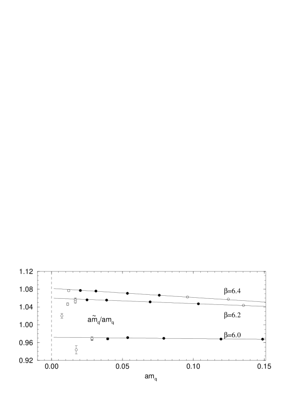
Figure 2.  : $a\widetilde{m}_{q}/am_{q}$ against $am_{q}$ for $O(a)$ improved fermions. Filled circles denote points used in the fits.

While there seems to be a reasonably linear relation between the two (lattice) definitions of the quark mass above $am_{s}$, below we again see deviations. This fit is somewhat sensitive to the value of $\kappa_{c}$ used; although the general picture shown in Fig. 2 never seems to change significantly. (Indeed using all the light quark data in the fit still produces a similar result.) This perhaps obscures the interpretation of Fig. 1 as being due to quenched chiral logarithms. Nevetheless, due to problems in determining $am_{q}$, we prefer to use the results with $a\widetilde{m}_{q}$, [8].

To try to expose the small quark region, and to determine $\delta$ (if the deviations are due to quenched chiral logarithms) then it is convenient to plot the logarithm of Fig. 1. This is done in Fig. 3,

Figure 3.  : $\ln[(a\widetilde{m}_{q}/(am_{\pi})^{2}]$ against $\ln[((r_{0}/a)^{2}\times(am_{ps})^{2}]$. The left line is a linear fit to the quarks with mass below the strange quark mass, while the dotted line is the previous fit from Fig. 1.

where we expect the slope to be $\delta$ (for the fitted quarks masses below the strange quark mass). We find for $\beta=6.0$, $\delta\sim 0.12(4)$, and for $\beta=6.2$, $\delta\sim 0.06(2)$ (for $\beta=6.4$ there is not enough data). For $\beta=6.0$, at least, there is reasonable agreement with the theoretical prejudice; for $\beta=6.2$ the value seems small.

Despite the above results it should be noted, as discussed above, that it is notoriously difficult to numerically detect quenched chiral logarithms. Indeed the above effects may simply be due to finite-size effects or ‘exceptional configuration’ problems. We have only been able to check very few quark mass points for finite size effects. The impression is that they are small; this is backed up by [8], who work on a larger lattice.

Exceptional configurations are seen as either the non-convergence of the fermion matrix inversion or the correlator seems to have a ‘fake source’ at some $t$ value. The problem is more severe for $O(a)$ improved fermions than for Wilson fermions and increases as $\beta\downarrow$ and/or $c_{sw}\uparrow$ and/or $m_{q}\downarrow$. (This is the main obstacle for the $O(a)$ improvement programme going below about $\beta\sim 6.0$.) The reason for this problem is due to the presence of small real eigenvalues in the fermion matrix. In an experiment, [9], we have chirally rotated the lattice quark mass, $am_{q}$, away from the real axis; the same configuration then gave a well behaved pion propagator. (We might then expect some mixing in the correlation function of the particle with its parity partner, however for the pion in the quark model this partner does not exist.) So perhaps simply throwing away the configuration does not affect the spectrum (?). It is desirable to have a crude indicator of whether we have an exceptional configuration. In [10] the simple proposal was made to look at the pion norm,

$$\Pi(\{U\})=\sum_{\vec{x},t}|\gamma_{5}G(\vec{x},t;\vec{0},0;\{U\})\gamma_{5}|^{2}.$$ (3)

(In our application, the source $(\vec{0},0)$ was also Jacobi smeared.) In Fig. 4,

Figure 4.  : The pion norm, eq. (3), against configuration number for $\beta=6.2$.

we show a sequence of pion norms for $\beta=6.2$. To decide on a criterion for an exceptional configuration (ie a spike in the pion norm) is not so easy. Some are obvious, for example from the pictures we have at $\kappa=0.1354$, $n_{conf}=217$ a problem. (The corresponding pion propagator is shown in [9].) Closer to the critical point than here more spikes have been seen in Wilson data, [11]. To be safe, we have actually chosen a more conservative local criterion where if at any $t$ value the (pion) correlation function fluctuates more than $5$ standard deviations from the local average we reject the configuration. This leads at $\beta=6.2$, $32^{3}\times 64$ for $\kappa=0.1352$, $0.1354$, $0.13555$ to rejection rates of about $2$, $4$ and $6\%$ respectively. (For the latter two $\kappa$ values about $15\%$ and $33\%$ of these rates were actually due to non-convergence of the inverter.) So in conclusion: while we feel that for any lighter quark mass than those considered here exceptional configurations become a real problem, at our masses while they are a nuisance, they do not distort the numerical result.

We now turn to a consideration of the decay constant $f_{ps}$. From eq. (1) we expect that $af_{ps}$ has no quenched chiral singularity in it, while $a^{2}g_{P}$ diverges in the chiral limit. In Fig. 5

Figure 5.  : Unrenormalised (improved) $af_{ps}$ versus the pseudoscalar mass.

we plot the unrenormalised $af_{ps}$. The results seem smooth over the whole quark mass range, with no singular behaviour. Looking at the ratio $af_{ps}/a^{2}g_{P}$ we see the same behaviour as in Fig. 1, ie for smaller quark masses than the strange quark mass a bend is seen in the data. As $af_{ps}/a^{2}g_{P}\propto[(am_{ps})^{2}]^{\delta}$ then taking the logarithm gives a direct estimate of $\delta$. In Fig. 6

Figure 6.  : Unrenormalised (improved) $\ln[af_{ps}/a^{2}g_{P}]$ against $\ln[((r_{0}/a)^{2}\times(am_{ps})^{2}]$. The left line is a linear fit to the results for quarks with mass below the strange quark mass. The same notation as for Fig. 3.

we show this, with fit values $\delta\sim 0.10(3)$ ($\beta=6.0$) and $\delta\sim 0.05(2)$ ($\beta=6.2$) consistent with the previous results.

Finally we consider chiral extrapolations of the nucleon and rho masses. In Figs. 7, 8

Figure 7.  : $am_{\rho}$ versus the pseudoscalar mass. The same notation as for Fig. 1. The fit function is given in eq. (4).

Figure 8.  : $am_{N}$ versus the pseudoscalar mass. The same notation as for Fig. 7.

we show the results, together with a phenomenological fit

$$(am_{\rho,N})^{2}=b_{0}+b_{2}(am_{ps})^{2}+b_{3}(am_{ps})^{3}.$$ (4)

In distinction to eq. (2) this does not have a quenched linear chiral term. (As there is curvature in the results above the strange quark mass, we have considered $(am_{\rho,N})^{2}$ rather than $am_{\rho,N}$ and included a cubic term in eq. (4). This gave a better fit function for the data.) While, for the nucleon this gives a good description of the data over the whole quark mass range and it is thus difficult to say in this case whether a linear term is necessary or not, the $\rho$ data might be showing some deviations for small quark masses.

4 Conclusions

Our main conclusion is that in quenched QCD there seems to be a dangerous region for quark masses $m_{q}\mathrel{\hbox to0.0pt{\lower 4.0pt\hbox{\hskip 1.0pt$\sim$}\hss}\raise 1.0pt\hbox{$<$}}m_{s}$. If we are interested in the strange quark mass or particles such as $m_{K}$, $m_{K^{*}}$, $\ldots$, or decay constants such as $f_{K}$, $f_{K^{*}}$, $\ldots$, this does not represent a problem. For quantities involving only the $u$ and $d$ quarks, it is probably best to adopt the pragmatic approach of making fits for $m_{q}\mathrel{\hbox to0.0pt{\lower 4.0pt\hbox{\hskip 1.0pt$\sim$}\hss}\raise 1.0pt\hbox{$>$}}m_{s}$ and then to extrapolate this to $m_{q}\sim m_{u/d}$, ie to chiral limit. (See, for example, the results for the quark mass, [7].) Evidence for chiral quenched logarithms is mixed – the best signal seems to be for the pion and its associated decay constant. Other channels seem to be less unambiguous. Indeed, as detecting and measuring quenching effects can be quite difficult this would indicate that the quenched approximation often seems to be working quite well.

The above results should be regarded as preliminary. We hope to present full results shortly, [12], including continuum extrapolations (considered in the talk, but not described here).

References

- [1] A. Ali Khan, S. Aoki, G. Boyd, R. Burkhalter, S. Ejiri, M. Fukugita, S. Hashimoto, N. Ishizuka, Y. Iwasaki, K. Kanaya, T. Kaneko, Y. Kuramashi, T. Manke, K. Nagai, M. Okawa, H. P. Shanahan, A. Ukawa, T. Yoshié, hep-lat/9909050.
- [2] C. Bernard, M. Golterman, Phys. Rev. D46 (1992) 853, hep-lat/9204007.
- [3] S. Sharpe, Phys. Rev. D46 (1992) 3146, hep-lat/9205020.
- [4] R. Gupta, Nucl. Phys. Proc. Suppl. 42 (1995) 85, hep-lat/9412078.
- [5] M. Booth, G. Chiladze, A. F. Falk, Phys. Rev. D55 (1997) 3092, hep-ph/9610532.
- [6] J. N. Labrenz, S. R. Sharpe, Phys. Rev. D54 (1996) 4595, hep-lat/9605034.
- [7] M. Göckeler, R. Horsley, H. Oelrich, D. Petters, D. Pleiter, P. E. L. Rakow, G. Schierholz, P. Stephenson, hep-lat/9908005.
- [8] S. Aoki, G. Boyd, R. Burkhalter, S. Ejiri, M. Fukugita, S. Hashimoto, Y. Iwasaki, K. Kanaya, T. Kaneko, Y. Kuramashi, K. Nagai, M. Okawa, H. P. Shanahan, A. Ukawa, T. Yoshié, hep-lat/9904012.
- [9] M. Göckeler, A. Hoferichter, R. Horsley, D. Pleiter, P. Rakow, G. Schierholz, P. Stephenson, Nucl. Phys. Proc. Suppl. 73 (1999) 889, hep-lat/9809165.
- [10] A. Hoferichter, V. K. Mitrjushkin, M. Müller–Preussker, Z. Phys. C74 (1997) 541, hep-lat/9506006.
- [11] A. Hoferichter, private communication.
- [12] M. Göckeler et al., in preparation.