[

Quasi-asymptotic freedom in the two dimensional $O(3)$ model

Abstract

The behavior of the renormalized spin 2-point function in the $O(3)$ and dodecahedron spin model are investigated numerically. The Monte Carlo data show excellent agreement between the two models. The short distance behavior comes very close to standard theoretical expectations, yet it differs significantly from it. A possible explanation of this situation is offered.

11.25.Bt, 11.15.Ha, 75.10.Hk

]

Are two dimensional (2D) nonabelian $\sigma$-models asymptotically free? After more than two decades, the answer remains unclear, with lots of supportive evidence on both sides of the issue. The main point of this letter is to provide some fresh evidence that even though the orthodox picture provides an excellent description of physics at intermediate momemta and distances not too short, it is in fact incorrect, a situation which I belive occurs also in $QCD_{4}$.

To that end I will present the result of Monte Carlo (MC) investigations of the continuum limit of the spin 2-point function in four spin models: i) Ising model, ii) $O(2)$ model, iii) $O(3)$ model and iv) dodecahedron spin model. As I will show, there is strong numerical evidence that the continuum limit of the dodecahedron spin model is identical to that of the $O(3)$ model. Undergoing a freezing transition at nonzero temperature, the latter is not likely to be asymptotically free. Moreover the continuum limit of the spin 2-point function of the $O(3)$ model disagrees with the PT formula with the value of $\Lambda/m$ predicted by Hasenfratz, Maggiore and Niedermayer based on the thermodynamic Bethe ansatz [1] and the normalization constant fixed by the scaling hypothesis of the form factor approach proposed by Balog and Niedermaier (BN) [2].

The numerical data suggest that in all the four models investigated, the short distance behaviour of the spin 2-point function is of the form $1/x^{1/4}$.

As a biproduct of my investigation, I report also on the behavior of the critical exponent $\eta$, which probably equals 1/4 in all four models. The subject of logarithmic corrections to $\eta=1/4$ in the $O(2)$ model has been discussed in several recent papers [3],[4], [5],[6], since a theoretical prediction stemming from the perturbative renormalization group approach exists [7] and it is not clear that the data are consistent with it. As I will discuss shortly, the existence of a continuum limit obtainable from the lattice model via multiplicative renormalization, an assumption which seems to be corroborated by the numerics, suggests that no such logarithmic corrections are present.

I would like to begin by reviewing the intimate connection between the short distance behavior of the continuum spin 2-point function and the critical exponent $\eta$. First some definitions: let $P=(p,0)$ and
- Spin 2-point function $G(p)$:

$$G(p)={1\over L^{2}}\langle|\hat{s}(P)|^{2}\rangle;\ \ \hat{s}(P)=\sum_{x}e^{iPx}s(x)$$ (1)

- Magnetic susceptibility $\chi$:

$$\chi=G(0)$$ (2)

- Correlation length $\xi$:

$$\xi={1\over 2\sin(\pi/L)}\sqrt{(G(0)/G(1)-1)}$$ (3)

As the continuum spin 2-point function I will use the limit $\xi\to\infty$ of

$${G(x/\xi)\equiv{\langle s(0).s(x)\rangle\xi^{2}/\chi}}\ \$$ (4)

Let $z$ be the physical continuum distance ($z\equiv x/\xi$, limit $\xi\to\infty$); the exponents $\bar{\eta}$ and $\bar{r}$ are defined by requiring that in the limit $z\to 0$ the expression

$$G(z)z^{\bar{\eta}}{(log(z))}^{2\bar{r}}$$ (5)

is finite and different from 0. Let $\eta$ and $r$ be defined so that in the limit $\xi\to\infty$ the quantity

$${c_{\it kt}\equiv{\chi\over{\xi^{2-\eta}{log(\xi)}^{-2r}}}}$$ (6)

is finite and different from 0.

I would like to claim that the existence of a continuum limit with the short distance behaviour described by (5) requires $\eta=\bar{\eta}$ and $r=-\bar{r}$. Indeed in the continuum limit, the limit $z\to 0$ is reached by letting both $x\to\infty$ and $\xi\to\infty$ but $x/\xi\to 0$. In fact the same consideration shows that in the same limit the lattice spin 2-point function must have the property

$$\langle s(0).s(x)\rangle x^{\bar{\eta}}$$ (7)

goes to a finite nonzero constant (i.e. there are no logarithmic modifications).

The Kosterlitz [7] prediction is that $\bar{r}=-1/16$. Finite size scaling at the kt-point do indicate a negative $r$ though smaller in magnitude [6]. The paradox discussed by many [3], [5],[6] is that the thermodynamic data suggest a positive value for $r$ [4],[6]. As explained above this is consistent with the fact that $r=-\bar{r}$, rather than $r=\bar{r}$ as incorrectly claimed in the literature.

However the fact that eq.(7) requires the lattice spin 2-point function to decay as a pure power with no logarithmic corrections suggests that most likely $r=-\bar{r}=0$. Indeed while for $\xi<\infty$ eq.(7) is valid only for $x\ll\xi$, baring some nonuniformity, eq.(7) ought to be describing the large distance behaviour of the lattice spin 2-point function at the critical point.

Next I would like to discuss the main point of this paper, which concerns the asymptotic behaviour of the continuum spin 2-point function $G(z)$ at short distances. It is known that in the Ising model $\eta=1/4$ $r=0$. I stated above what perturbative renormalization group (RG) arguments predict for $O(2)$. For $O(3)$ similar arguments [8] predict $\eta=0$ $r=-1$. However when combined with the thermodynamic Bethe ansatz and the scaling hypothesis in the form factor approach, this latter prediction becomes even more precise [2] :

$$G(z) = {1.000034657\over 3\pi^{3}\,1.001687^{2}}(t+ln(t)$$ (8)

$$+ 1.1159+ln(t)/t+.1159/t)^{2},$$ (9)

where $t\equiv{-ln(z\Lambda)},\Lambda=e/8.$  I am not aware of any predictions regarding $\eta$ and $r$ for the dodecahedron spin model.

In Fig.1 I present my Monte Carlo results for $G(z)z^{1/4}$ for (in rising order) Ising, $O(3)$ and $O(2)$; I also show the curve for free field (lowest curve) and the PT curve with the normalization constant predicted by Balog and Niedermaier (upper curve) [2]. The MC data were taken at $\xi\sim 167$ and L=1230. They represent the on axis correlation and I will discuss shortly the lattice artefacts. For now I would like to make the following observations:
1.    In all three models $G(z)$ approaches the free field value for $z\to\infty$, as required by the Orstein-Zernke behaviour [9].
2.   For $z\geq.05$ $G(z)$ in the three models behaves quite similarly.
3.   The data suggest that in all three models $\eta=1/4$, but that compared to the Ising model the short distance behavior may be more singular in $O(2)$ and less singular in $O(3)$. This is would be consistent with a negative $\bar{r}$ in $O(2)$ but a positive one in $O(3)$ (although the data are also consistent with $\bar{r}=0$).
4.   Even though for $.02<z<.1$ the difference with the BN refined PT curve is small (about 2$\%$), it is clearly there and, as I will indicate next, it is not a lattice artefact.

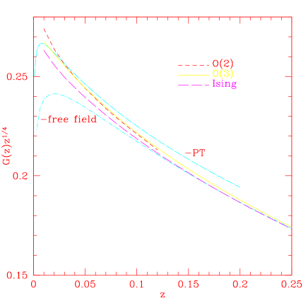
FIG. 1.: Spin 2-point function $G(z)$ versus physical distance $z$ for the Ising, $O(3)$ and $O(2)$ models. Also shown the free field curve and the BN refined PT curve for $O(3)$.

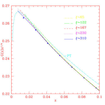
FIG. 2.: Spin 2-point function $G(z)$ versus physical distance $z$ for the $O(3)$ model at several correlation lengths. Also shown the BN refined PT curve.

In Fig.2 I present the MC results for the $O(3)$ model for $\xi$ ranging from 65 to 310. The error bars are about .3$\%$, too small to show. The data were produced using Wolff’s method [10]. At each $\beta$ and $L$ value, at least five independent runs were made and the error estimated using the jack-knife method. The primary source of error are the values of $\chi$ and $\xi$, whose determination involves large distances. To give a feeling for the size of the lattice artefacts, for $\xi\sim 310$ the (solid) curve represents $G(z)$ on axis while the points $G(z)$ along the diagonal. Both this test and the good agreement of these data with the data at $\xi\sim 230$ suggest that, barring some very slow drift, the continuum limit has been reached for $z\geq.03$. The continuum values are clearly off the BN refined PT curve (upper curve).

As explained above, the critical behaviour of $\chi$ and $\xi$ carry relevant information regarding the short distance behaviour of $G(z)$. In Fig.3 I represent $ln(\chi)-1.75ln(\xi)$. The upper curve represents the MC data. The lower (dashed) curve represents the ratio of the values of this quantity computed via the BN formula

$${\chi\over\xi^{2}}={3\pi\,1.001687^{2}\over{4\,1.000034657\,\beta^{2}}}\left\{1+{.1816\over\beta}+{.133\over\beta^{2}}+{.1362\over\beta^{3}}\right\}$$ (10)

over its MC values. A correct prediction of the BN formula would require the dashed curve to approach 1 for $\xi\to\infty$. The data produce a (dashed) curve which is not flat and which seems to approache the line at 1 with a nonzero slope.

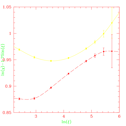
FIG. 3.: $ln(\chi)-1.75ln(\xi)$ versus $ln(\xi)$ for the $O(3)$ model. Dashed curve represents MC data combined with the BN bootstrap prediction, a correct prediction requiring convergence to 1 for $\xi\to\infty$.

The upper (solid) curve indicates that $r$ could be different from 0 and in fact negative. To determine whether there is a logarithmic modification to $\eta=1/4$ and obtain a precise value for $r$ one would need data at larger $\xi$. However the lack of smoothness of the curve suggests that the errors are underestimated already at $\xi\sim 310$ (probably due to critical slowing down).

The last piece of numerical evidence which suggests that $O(3)$ is not asymptotically free comes from a comparison of its spin 2-point function with that of of the dodecahedron spin model. This is shown in Fig. 4, which shows $G(z)$ for the latter model at $\xi\sim 11,19,34,66$ and 120 (broken line) and $G(z)$ for the $O(3)$ model at $\xi\sim 122$ (solid line on axis, dots on the diagonal). As the correlation length increases, $G(z)$ for the dodecahedron model approaches that of $O(3)$ and at $\xi\sim 120$ the two curves are practically indistinguishable for $z\geq.04$. It appears rather certain that the two models share the same $G(z)$ in the continuum limit. However, as already mentioned, it is highly unlikely that the dodecahedron model, undergoing freezing at finite $\beta$, exhibits asymptotic freedom.

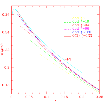
FIG. 4.: Spin 2-point function $G(z)$ in the dodecahedron model for several correlation lengths. Also shown $G(z)$ for the $O(3)$ model at $\xi\sim 122$ and the BN refined PT curve.

$\it Discussion$

1. I believe the numerical evidence presented above suggests that in the $O(3)$ nonlinear $\sigma$ model the short distance behaviour of $G(z)$ corresponds to $\bar{\eta}=1/4$, $\bar{r}\geq 0$.

2. Perturbative renormalization group arguments predict that in all $O(N)$ models $N\geq 3$ $\eta=0$, $\bar{r}$ is negative and varies monotonically with $N$ from -1 for $O(3)$ to -1/2 for $O(\infty)$. Based on the observed behavior of $O(3)$ I would conjecture that for all $3\leq N<\infty$ $\eta=1/4$. Since the spherical model $O(\infty)$ has $\eta=0$, $\bar{r}=-1/2$, such a scenario would correspond to a nonuniformity of the $1/N$ expansion. The uniformity of the $1/N$ expansion for $\beta\to\infty$ has been questioned before [11].

3. Since for $.02\leq z\leq.1$ the deviation from the BN refined PT prediction is 2$\%$ or less, one may wonder why that is so? I think the answer is in Fig.1, where I compare $G(z)$ for different models. Please note that the free field curve describes also the spherical model and $G(z)$ for it is quite close to that of $O(3)$ for $z$ not too small. It is well known [12] that the $1/N$ expansion is legitimate at fixed $\tilde{\beta}\equiv{\beta\over N}$ and the only issue [11] is whether this expansion is uniform for $\tilde{\beta}\to\infty$. The reason the orthodoxy comes so close to the truth is two fold: i) the fast convergence of the $1/N$ expansion for moderate $\tilde{\beta}$ and ii) the large value of $\beta_{crt}$. Thus, even though I believe both the $1/N$ expansion and perturbation theory are nonuniform, they come very close to the truth at moderate correlation length. Since for distances not too small or momenta not too large the continuum limit is well described at moderate $\xi$ values, the orthodoxy will describe correctly physics at such distances and/or momenta. It is only at short distances or large momenta that the true test of the orthodoxy can be performed.

4. Until now I discussed only some new numerical information. Some readers, such as those who recently wrote ‘We believe however that the continuing accumulation of unambiguous, consistent and increasingly accurate numerical support for the RG predictions from a variety of independent approaches leaves liitle if any space for alternative pictures.’ [13], may not find my numerical evidence conclusive. I will invite them then to reconsider the two theoretical arguments advanced by Patrascioiu and Seiler regarding the existence of a massless phase in all $O(N)$ models:

i) We showed rigorously [14] that if a certain cluster, baptized the equatorial cluster, does not percolate, the model must be massless. We also advanced some nonrigorous arguments why that cluster did not seem likely to percolate [15]. After seven years since those arguments were advanced, no mathematical physicist has proved the contrary or given us an example of how this equatorial cluster might percolate (see Open Problems in Mathematical Physics, http://www.iamp.org). Can any skeptical reader give such an example?

ii) We also showed rigorously that among smooth configurations, the dominant ones must be the superinstantons [16] not the much publicized instantons. But in a superinstanton configuration there is a ring of arbitrary size in which the spin points roughly in a certain direction. Hence in such a configuration, the inverse image of a small patch of the sphere will form a ring and hence the equatorial cluster will not percolate. Therefore the existence of superinstantons as the dominant configuration at weak coupling reinforces the argument for the existence of a massless phase and hence the absence of asymptotic freedom in the massive phase.

I think irrespective of any numerics, to paraphrase Butera and Comi [13], ‘the two arguments mentioned above leave little if any space for the standard picture to be correct’.

5. Even though strictly incorrect, the standard picture provides an excellent phenomenological description at distances not too small ($z>.02$) or momenta not too large ($p<2\pi/.02\sim 300$. This is not something never seen before. Indeed it is taught in every course in Quantum Mechanics that the probability to find a particle trapped in a potential well (say an $\alpha$-particle) decays exponentially in time. The time constant of that exponential is called the life time of the state, and innumerable experiments over the years have measured such life times. I am not aware of anybody ever having claimed to have detected deviations from this alleged exponential law. Yet it is a mathematical fact that if the particle decays at all, the large time asymptotic behavior cannot be exponential, but some inverse power of the time [17]. This fact is little known in the physics community (witness the many papers by particle physicists computing the lifetime of the ‘false cosmological vacuum’) because in fact the exponential law describes very well the data. My claim is that a similar situation occurs in the 2D nonlinear $\sigma$ models (and probably $QCD_{4}$): even though eventually, at $\beta$ sufficiently large superinstantons win and render the model massless, at moderate values of $\beta$ such as $\beta=2$ for $O(3)$, instantons (localized defects) dominate the typical configuration, which behaves very much as predicted by perturbation theory and/or the $1/N$ expansion. Only by probing sufficiently small distances or large momenta should one be able to detect major deviations from the expected behavior.

These ideas stem from my long term collaboration with Erhard Seiler and were crystalized by my recent collaboration with J.Balog, M.Niedermaier, F.Niedermayer and P.Weisz.

REFERENCES

- [1] P.Hasenfratz, P.Maggiore and F.Niedermayer, Phys.Lett. B 245 (1990) 522.
- [2] J.Balog and M.Niedermaier,Nucl.Phys. B500 (1997) 421, Phys.Rev.Lett. 78 (1997) 4151.
- [3] R.Kenna and A.C.Irving, Phys.Lett B351 (1995) 273.
- [4] A.Patrascioiu and E.Seiler, Phys.Rev. B54 (1996) 7177.
- [5] M.Campostrini, A.Pelissetto, P.Rossi and E.Vicari, Phys.Rev. D54 (1996) 1782.
- [6] W.Janke, Logarithmic corrections in the 2D XY model, preprint KOMA-96-17, hep-lat/9609045
- [7] J.M.Kosterlitz, J.Phys. C7 (1974) 1046
- [8] A.M.Polyakov, Phys.Lett. 59B (1975) 79, E.Brezin and J.Zinn-Justin Phys.Rev.Lett. 36 (1976) 691
- [9] J.Bricmont and J.Fröehlich Comn.Math.Phys. 98 (1985) 553
- [10] U.Wolff, Nucl.Phys. B334 (1990) 581.
- [11] A.Patrascioiu and E.Seiler, Nucl.Phys. B443 (1995) 596.
- [12] A.Kupianen, Commun.Math.Phys. 73 (1980) 273.
- [13] P.Butera and M.Comi, Phys.Rev. B54 (1996) 15828.
- [14] A.Patrascioiu and E.Seiler, J.Stat.Phys. 69 (1992) 573
- [15] A.Patrascioiu, Existence of algebraic decay in nonabelian ferromagnets ……., AZPH-TH/91-49 math-ph/0002028, A.Patrascioiu and E.Seiler Nucl.Phys. (Proc.Suppl.) B30 (1993) 184.
- [16] A.Patrascioiu and E.Seiler, Phys.Rev.Lett. 74 (1995) 1920.
- [17] L.A.Kalfin, Zh.Eksp.Teor.Fiz. 33 (1957) 1371, …………. A.Patrascioiu, Phys.Rev. D24 (1981) 406.