Determinant of a new fermionic action on a lattice - (I)

Abstract

We investigate, analytically and numerically, the fermion determinant of a new action on a (1+1)-dimensional Euclidean lattice. In this formulation the discrete chiral symmetry is preserved and the number of fermion components is a half of that of Kogut-Susskind. In particular, we show that our fermion determinant is real and positive for U(1) gauge group under specific conditions, which correspond to gauge conditions on the infinite lattice. It is also shown that the determinant is real and positive for SU(N) gauge group without any condition.

I Introduction

As the Nielsen-Ninomiya theorem [1] states, we necessarily meet the difficulty of so-called fermion doubling problem when we formulate fermion fields on a lattice. In practical calculations, Wilson fermions [2] have been widely used, where an additional term which vanishes in the naive continuum limit is introduced at the expense of the chiral symmetry. An alternative scheme was proposed by Kogut and Susskind [3]. In this scheme the chiral symmetry is maintained as discrete one and doubler fermions are regarded as fermions in other species. In $(1+D)$ dimensions, the Kogut-Susskind (KS) formalism describes a theory with $2^{\frac{1+D}{2}}$ degenerate quark flavors ($2^{1+D}$ components).

Recently it has been shown that lattice fermionic actions satisfying the Ginsparg-Wilson relation [4] may provide a solution of the chirality problem [5]. In these attempts the modified chiral symmetry operator is used in stead of $\gamma_{5}$. The actions are local in the sense that the fermionic matrix are bounded by $Ce^{-\gamma\mid x\mid}$. However, it has been proved that actions with the Ginsparg-Wilson relation cannot be ”ultralocal” [6]. From the practical point of view, the ultralocality (the couplings drop to zero beyond a finite number of lattice spacings) is also important. Thus ultralocal fermionic actions with better features than, for example, the KS action is awaited, though not a final solution of the chirality problem.

In the recent papers [7, 8], we proposed a new type of fermionic action on a $(1+D)$-dimensional lattice. The action is ultralocal and constructed so that fermion fields satisfy the bosonic type of dispersion relation. In this sense there are no extra poles in the propagator. We found that the minimal number of fermion components, dimensions of the spinor space, is $2^{D-1}$ in the Minkowski case and $2^{D}$ in the Euclidean case, which should be compared with $2^{1+D}$ of the KS fermion. Furthermore our action has the discrete chiral symmetry as well.

It is much of interest to investigate the numerical feasibility of our new fermionic action. When dynamical fermions are included, the property of fermion determinants is crucial in numerical calculations. For example, some methods proposed to treat fermionic freedoms rely on reality or positivity of the fermion determinants [9].

In this paper we report the analytical and numerical results on the fermion determinants of our new action in $(1+1)$ dimensions. Our main concern is on U(1) gauge group, but some results on SU(N) gauge group are also presented. In the case of U(1) gauge group, we will see that calculations with specific conditions for temporal link variables are stable and satisfactory though results without the conditions are unstable. The reason why we need those conditions will be discussed in detail.

In Sec.2, we recapitulate our formalism for later convenience. The analytical and numerical results on fermion determinants will be presented in Sec.3, which is followed by the summary.

II New fermionic action

In the previous paper [8], we proposed a new fermionic action on the Euclidean lattice. Though the action respects the discrete chiral symmetry like one in the KS action, fermion fields in this action have $2^{D}$ components in $(1+D)$ dimensions, which should be compared with $2^{1+D}$ in the case of KS fermions. In this section we briefly sketch our formalism for later convenience.

The action can be written with the fermion matrix $\Lambda$ as

$$S_{f}=\sum_{m,n}\psi^{\dagger}_{m}\Lambda_{m,n}\psi_{n},$$ (1)

where the summation is over lattice points and spinor indices, and our fermion matrix is defined by

$$\Lambda=1-S_{0}^{\dagger}U_{E}.$$ (2)

Here $U_{E}$ is the Euclidean time evolution operator and $S_{\mu}$ is the unit shift operator defined as

$$S_{\mu}\psi(x^{0},x^{1},\ldots,x^{\mu},\ldots,x^{D})=\psi(x^{0},x^{1},\ldots,x^{\mu}+1,\ldots,x^{D})\qquad(\mu=0,1,\ldots,D).$$ (3)

We required that the propagator has no extra poles and found that $U_{E}$ has the form

$$U_{E}=1-\sum_{i=1}^{D}\frac{r_{E}}{2}\left\{iX_{i}\left(S_{i}-S_{i}^{\dagger}\right)+\left(1-Y_{i}\right)\left(S_{i}-2+S_{i}^{\dagger}\right)\right\},$$ (4)

where $r_{E}$ is the ratio of the temporal lattice constant to the spatial one and $X$’s and $Y$’s, which are matrices with respect to spinor indices, should satisfy the following algebra:

$$\left\{\begin{array}[]{ccl}\left\{X_{i},X_{j}\right\}&=&\displaystyle{\frac{2}{r_{E}}}\delta_{ij},\\ \left\{X_{i},Y_{j}\right\}&=&0,\\ \left\{Y_{i},Y_{j}\right\}&=&2\left(\displaystyle{\frac{1}{r_{E}}}\delta_{ij}+1\right),\end{array}\right.$$ (8)

where $i$ and $j$ run from $1$ to $D$. The matrix $2(\delta_{ij}/r_{E}+1)$ is positive definite for any positive $r_{E}$, therefore $X$’s and $Y$’s can be assumed hermitian,

$$X_{i}^{\dagger}=X_{i},\qquad Y_{i}^{\dagger}=Y_{i}.$$ (9)

The matrices $X$’s and $Y$’s are written in terms of the Clifford algebra $\Gamma_{1},\Gamma_{2},\ldots,\Gamma_{2D}$ as

$$X_{i}=\displaystyle{\frac{\Gamma_{i}}{\sqrt{r_{E}}}},\qquad Y_{i}=\displaystyle{\sum_{j=1}^{D}}\alpha_{ij}\Gamma_{D+j},$$ (10)

where

$$\Gamma_{i}^{\dagger}=\Gamma_{i},\qquad\left\{\Gamma_{i},\Gamma_{j}\right\}=2\delta_{ij}\qquad(i,j=1,\ldots,2D),$$ (11)

and $\alpha_{ij}$ are certain real constants. The dimension of the irreducible representation for $\Gamma$’s is $2^{D}$ and accordingly $\psi$ has $2^{D}$ components.

Now we give some useful properties of the time evolution operator $U_{E}$. We can see immediately that

$$U_{E}^{\dagger}=U_{E},$$ (12)

as $X$’s and $Y$’s are hermitian. Since the inverse of $U_{E}$ is given by

$$U_{E}^{-1}=1-\sum_{i=1}^{D}\frac{r_{E}}{2}\left\{-iX_{i}\left(S_{i}-S_{i}^{\dagger}\right)+\left(1+Y_{i}\right)\left(S_{i}-2+S_{i}^{\dagger}\right)\right\},$$ (13)

we find that $U_{E}$ is related to its inverse as:

$$\Gamma_{2D+1}U_{E}\Gamma_{2D+1}=U_{E}^{-1},$$ (14)

where

$$\Gamma_{2D+1} \equiv i\Gamma_{1},\Gamma_{2}\ldots\Gamma_{2D},$$ (15)

$$\Gamma_{2D+1}^{\dagger}=\Gamma_{2D+1},\qquad\Gamma_{2D+1}^{2}=1, \qquad\left\{\Gamma_{i},\Gamma_{2D+1}\right\}=0\qquad(i=1,\cdots,2D).$$ (16)

The interaction of the fermion with gauge fields is introduced by replacing the unit shift operators by covariant ones:

$$S_{\mu}\to S_{\mu}(x)\equiv U_{x,x+\hat{\mu}}S_{\mu},$$ (17)

where $\hat{\mu}$ is the unit vector along the $\mu$’th direction, and $U_{x,y}$ is a link variable connecting sites $x$ and $y$.

The fermion matrix Eq.(2) and the time evolution operator Eq.(4) become

$$\Lambda(x)=1-S_{0}^{\dagger}(x)U_{E}(x),$$ (18)

and

$$U_{E}(x)=1-\sum_{i=1}^{D}\frac{r_{E}}{2}\left\{iX_{i}\left(S_{i}(x)-S_{i}^{\dagger}(x)\right)+\left(1-Y_{i}\right)\left(S_{i}(x)-2+S_{i}^{\dagger}(x)\right)\right\}.$$ (19)

With gauge fields coupled to the fermions, however, Eqs.(13) and (14) do not hold any more in arbitrary dimensions except for $(1+1)$ dimensions. In $(1+1)$ dimensions these relations are

$$U_{E}^{-1}(x)=1-\frac{r_{E}}{2}\left\{-iX_{1}\left(S_{1}(x)-S_{1}^{\dagger}(x)\right)+\left(1+Y_{1}\right)\left(S_{1}(x)-2+S_{1}^{\dagger}(x)\right)\right\},$$ (20)

and

$$\Gamma_{3}U_{E}(x)\Gamma_{3}=U_{E}^{-1}(x),$$ (21)

which are used in the next section.

III Analytical and numerical results of our fermion determinant in $(1+1)$ dimensions

A Reality of the determinant

In this section we show the analytical and numerical results of our fermion determinant in the $(1+1)$-dimensional case.

First, we investigate the determinant of the unit shift operator $S_{0}(x)$ in $(1+D)$ dimensions. Let us denote the link variables by $U_{x,x+\hat{\mu}}$ which live on the links connecting two neighboring lattice sites $x$ and $x+\hat{\mu}$. Now we consider the case of the Abelian gauge group U(1), and they can be written in the form

$$U_{x,x+\hat{\mu}}=e^{i\theta_{\mu}(x)},$$ (22)

where $\theta_{\mu}(x)$ is restricted to the compact domain [0, 2$\pi$).

Then, $S_{0}(x)$ can be constructed as a $N_{T}N_{{\mbox{\boldmath$x$}}}N_{s}\times N_{T}N_{{\mbox{\boldmath$x$}}}N_{s}$ matrix where $N_{T}$ and $N_{{\mbox{\boldmath$x$}}}$ is the size of the lattice in the Euclidean time and the spatial directions, respectively, and $N_{s}$ is the number of spinor components. $S_{0}(x)$ is diagonal in the spatial and spinor space and consists of block $N_{T}\times N_{T}$ matrices $Q({\mbox{\boldmath$x$}})$ belonging to the Euclidean time space. Thus we can write the determinant of $S_{0}(x)$ as follows:

$$\det S_{0}(x)=\left|\begin{array}[]{cccccc}Q(1)&&&&&\\ &\ddots&&&&\\ &&Q(2)&&&\\ &&&\ddots&&\\ &&&&Q(N_{\mbox{\boldmath$x$}})&\\ &&&&&\ddots\\ \end{array}\right|,$$ (29)

where $Q({\mbox{\boldmath$x$}})$ for each $x$ appear $N_{s}$ times as $S_{0}(x)$ is unity in the spinor space.

The determinant of $Q({\mbox{\boldmath$x$}})$ is easily calculated by noticing its matrix form:

$$\det Q({\mbox{\boldmath$x$}}) = \left|\begin{array}[]{ccccc}0&U_{(1,{\mbox{\boldmath$x$}}),(2,{\mbox{\boldmath$x$}})}&&&\\ &0&U_{(2,{\mbox{\boldmath$x$}}),(3,{\mbox{\boldmath$x$}})}&&\\ &&\ddots&\ddots&\\ &&&0&U_{(N_{T-1},{\mbox{\boldmath$x$}}),(N_{T},{\mbox{\boldmath$x$}})}\\ -U_{(N_{T},{\mbox{\boldmath$x$}}),(1,{\mbox{\boldmath$x$}})}&&&&0\\ \end{array}\right|$$ (35)

$$= (-)^{N_{T}-1}U_{(1,{\mbox{\boldmath$x$}}),(2,{\mbox{\boldmath$x$}})}U_{(2,{\mbox{\boldmath$x$}}),(3,{\mbox{\boldmath$x$}})}\ldots\left(-U_{(N_{T},{\mbox{\boldmath$x$}}),(1,{\mbox{\boldmath$x$}})}\right)$$ (36)

$$= (-)^{N_{T}}\exp\left\{i\sum_{t=1}^{N_{T}}\theta_{0}(t,{\mbox{\boldmath$x$}})\right\}.$$ (37)

We used the anti-periodic boundary condition for the time direction, which is represented by a negative sign in the lower-left corner of the matrix $Q$.

As a result, in $(1+D)$ dimensions we find

$$\det S_{0}(x) = \prod_{{\mbox{\boldmath$x$}}}\left[(-)^{N_{T}}\exp\left\{i\sum_{t=1}^{N_{T}}\theta_{0}(t,{\mbox{\boldmath$x$}})\right\}\right]^{N_{s}}$$ (38)

$$= \exp\left\{iN_{s}\sum_{t}\sum_{{\mbox{\boldmath$x$}}}\theta_{0}(t,{\mbox{\boldmath$x$}})\right\}=e^{i\alpha},$$ (39)

where the angular variable $\alpha$ is defined by

$$\alpha=N_{s}\sum_{t}\sum_{{\mbox{\boldmath$x$}}}\theta_{0}(t,{\mbox{\boldmath$x$}}).$$ (40)

From now we assume $D=1$ and show that the determinant of the Euclidean time evolution operator $U_{E}(x)$ is unity. By Eq.(21) we easily find $\det U_{E}(x)=\pm 1$. Since $X$’s and $Y$’s obey Eq.(10) and in the limit $r_{E}\to 0$

$$r_{E}X_{i}\longrightarrow 0,\qquad r_{E}Y_{i}\longrightarrow 0,$$ (41)

$\det U_{E}(x)$ is equal to $1$ at $r_{E}=0$. From the continuity of $\det U_{E}(x)$ with respect to $r_{E}\geq 0$, we conclude

$$\det U_{E}(x)=1,$$ (42)

in the $(1+1)$-dimensional case.

Collecting the above results, the relations (21) and (42), and the hermiticity of $U_{E}(x)$, we can obtain a relation on the phase of our fermion determinant in $(1+1)$ dimensions as follows:

$$\left(\det\Lambda(x)\right)^{\ast} = \det\left(1-S_{0}^{\dagger}(x)U_{E}(x)\right)^{\dagger}=\det\left(1-U_{E}(x)S_{0}(x)\right)$$ (43)

$$= \det U_{E}(x)\det S_{0}(x)\det\left(S_{0}^{\dagger}(x)U_{E}(x)^{-1}-1\right)$$ (44)

$$= (-)^{\mbox{dim. of $\Lambda$}}\det S_{0}(x)\det\Lambda(x).$$ (45)

Since the number of components of our fermion is $N_{s}=2$ and consequently the fermion matrix $\Lambda(x)$ always has an even number of dimensions, we get

$$\left(\det\Lambda(x)\right)^{\ast}=e^{i\alpha}\det\Lambda(x).$$ (46)

Accordingly in the case of $(1+1)$ dimensions with U(1) gauge fields, our fermion determinant is real under the condition

$$\alpha=2\pi n\qquad\mbox{($n$: integer)},$$ (47)

where $\alpha$ is defined in Eq.(40). The condition specified by Eq.(47) will be called ”GT-condition” in this paper, where the temporal link variables are globally constrained as $\sum_{x}\theta_{0}(x)=\pi n$ and on the infinite lattice the condition is achieved by a gauge transformation. We also define ”T-condition” as $\theta_{0}(x)=0$, which corresponds to the temporal gauge condition on the infinite lattice.

At a glance, it seems strange that the determinant has $\alpha$-dependence, because $\alpha$ can be gauged away. However, this is not true for a finite lattice, since all gauge transformations on the infinite lattice are not allowed on a finite lattice with periodic boundary conditions. Thus, the dependence comes from finiteness of the lattice. For example, $\sum_{t}\theta_{0}(t,{\mbox{\boldmath$x$}})$ is invariant under any gauge transformation on a finite lattice with periodic boundary conditions. The temporal gauge condition is certainly a consistent gauge in an infinite system, but not in a finite system. However, this restriction is just an artifact arising when we try to approximate an infinite system by a finite one. We could think in the following way. Given an infinite system, we impose the temporal gauge condition, which is legitimate. Then we take an finite sub-system to approximate the original total system. The difference is due to size and boundary effects and would disappear in the infinite volume limit. The same is also true for the GT-condition. It should be noted that the fermion determinant is invariant under gauge transformations on a finite lattice, but the determinant does depend on our ”gauge conditions”: the T- or the GT-condition.

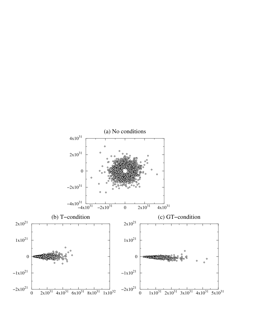
FIG. 1.: The distributions in the complex plane of our fermion determinants for each configuration of 2000 Monte Carlo iterations after getting good enough equilibrium, i.e. after 2000 iterations, on a $8\times 8$ lattice at $\beta=1.5$. Plots (a),(b) and (c) correspond to under no conditions, the T- and the GT-condition, respectively.

Now, we will give the numerical results in the $(1+1)$-dimensional U(1) gauge theory with our fermion action. In the following numerical simulations link variables are updated by the Metropolis method and determinants are calculated by the LU decomposition. So there are no systematic errors in the determinants. The way to generate a sequence of configurations in the Monte Carlo computation is as follows. In the T-condition, we fix $U_{0}(x)=1$ everywhere. After this, all temporal link variables are not changed and we only update the link variables of spatial direction using the Metropolis method. In the GT-condition, we prepare a configuration satisfying $\sum_{x}\theta_{0}(x)=\pi n$. Then a temporal link variable $e^{i\theta_{0}(x)}$ is replaced by $e^{i\theta_{0}(x)+i\chi}$, where $\chi$ is a random number between $-\pi$ and $\pi$. At the same time another temporal link variable, which is chosen randomly, is multiplied by $e^{-i\chi}$. And we use the above configuration as the trial one in a Metropolis acceptance test. It can be shown that this procedure satisfies the micro-reversibility requirement, and therefore also the detailed balance condition.

In Fig.1(a) - 1(c) we show the distribution of the fermion determinants in the complex plane for some $\beta$. The statistics is $2000$ thermalizations and $2000$ measurements. In Fig.1(a), no conditions are imposed on temporal link variables. Fig.1(b) is the result in the T-condition. In Fig.1(c), the GT-condition with $n=0$ is imposed, namely the condition $\alpha=0$ in Eq.(40) is always kept in Monte Carlo updates. The distribution in Fig.1(a) has a doughnut-like structure with a center around the origin, so that we can expect that the convergence for any observation is very poor. On the other hand, Fig.1(b) and 1(c) show that the determinants in the T- and the GT-condition are real as expected and also positive. The distribution in the imaginary direction is due to numerical errors (note the difference in the scales of real and imaginary parts). The positivity of determinants is important from the numerical point of view and will be discussed later.

To test the convergence in the above three types of conditions, we measured the expectation value of a plaquette value as a function of $\beta$ using the following formula:

$$\langle W_{p}\rangle=\frac{\displaystyle{\int dUd\psi d\psi^{\dagger}W_{p}e^{-S_{g}-S_{f}}}}{\displaystyle{\int dUd\psi d\psi^{\dagger}e^{-S_{g}-S_{f}}}}=\frac{\displaystyle{\int dUW_{p}\det\Lambda(x)e^{-S_{g}}}}{\displaystyle{\int dU\det\Lambda(x)e^{-S_{g}}}}=\frac{\displaystyle{\langle W_{p}\det\Lambda(x)\rangle}_{0}}{\displaystyle{\langle\det\Lambda(x)\rangle}_{0}}.$$ (48)

Here $S_{g}$ is the usual action for link fields, and $d\psi$, $d\psi^{\dagger}$ and $dU$ stand for $\prod_{x,\alpha}d\psi_{\alpha}(x)$, $\prod_{x,\alpha}d\psi^{\dagger}_{\alpha}(x)$ and $\prod_{x,\mu}dU_{x,x+\hat{\mu}}$, respectively.

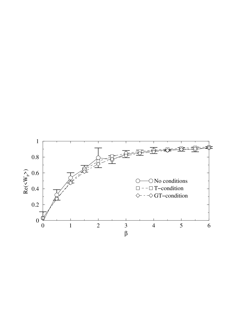
FIG. 2.: The real part of the averaged plaquette vs $\beta$ on a $8\times 8$ lattice.

In Fig.2 we can see that the expectation values in the T- and the GT-condition display gentle curves, while one without any conditions is spiky especially for small $\beta$. Here, the plotted points are the average over $10$ results, each of which is obtained by $2000$ Monte Carlo iterations at each $\beta$. And the error bars are evaluated by using the standard deviation of the $10$ results. If the error bars are not displayed, they are not visible at this scale.

The poorness of the convergence without any conditions can be traced back to the behavior of the denominator in Eq.(48). The expectation value $\langle\det\Lambda(x)\rangle_{0}$ not only takes complex values but also suddenly increases or decreases during sampling. Fig.3 shows the absolute value of the averaged fermion determinant as a function of the update iterations for each condition. We find that the convergence in the case of no conditions is ill while in the cases of other two conditions very fine. Generally the more iterations are expected to improve the convergence. Without any conditions, however, this is not the case since the expectation value of the determinant must be in the empty hole of a doughnut-like structure in Fig.1(a). Thus it is difficult to improve the convergence for any expectation value within a reasonable number of iterations.

Now what is the difference between the T- and the GT-condition? We expect that the GT-condition is superior to the T-condition since the former condition is much weaker condition than the latter. To see this, we show in Figs.4(a) and 4(b) the averaged plaquette value in the pure U(1) gauge theory as a function of $\beta$ for three types of conditions. We find the line without any conditions and one with the GT-condition are very close to each other, but the line calculated in the T-condition is slightly upper than those. As expected, this difference comes from the size effects in each condition and obviously tends to decrease as the lattice size becomes larger. Thus we conclude that the GT-condition has better feature on a finite lattice: the fermion determinant is positive and the finite-size effects are smaller.

FIG. 3.: The absolute value of the averaged fermion determinant vs Monte Carlo iterations. The data were computed using the same configurations as in Fig.1(a) - 1(c)

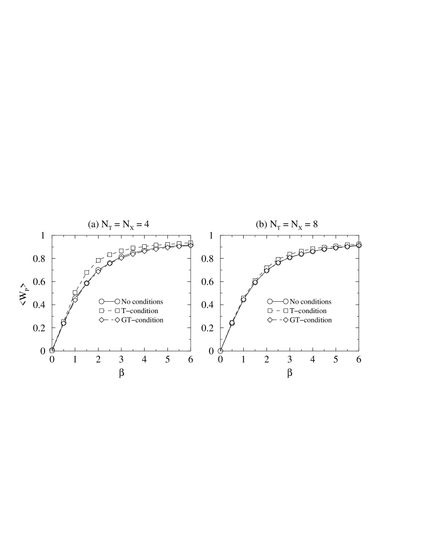
FIG. 4.: The averaged plaquette vs $\beta$ on a (a) $4\times 4$ and (b) $8\times 8$ lattice.

B Spectrum of the fermion matrix

Before discussing the positivity of the fermion determinant, we study the spectrum of $\Lambda(x)$. First, we introduce a discrete rotational symmetry in the complex plane for eigenvalues of $S_{0}^{\dagger}(x)U_{E}(x)$. Defining $(T)_{t,t^{\prime}}=\exp(i2\pi t/N_{T})\delta_{t,t^{\prime}}$, we find

$$TS_{0}^{\dagger}(x)U_{E}(x)T^{-1}=\exp\left(\displaystyle{i\frac{2\pi}{N_{T}}}\right)S_{0}^{\dagger}(x)U_{E}(x).$$ (49)

This relation implies that if $\lambda$ is some eigenvalue of $S_{0}^{\dagger}(x)U_{E}(x)$, then $\exp\left(i2\pi/N_{T}\right)\lambda$ is also its eigenvalue. Next using the following relation

$$\det\left(U_{E}(x)S_{0}(x)-\lambda^{\ast}\mbox{\bf{1}}\right) = \det\left(U_{E}(x)S_{0}(x)\right)\det\left(\mbox{\bf{1}}-\lambda^{\ast}S_{0}^{\dagger}(x)U_{E}(x)^{-1}\right)$$ (50)

$$= \det\left(U_{E}(x)S_{0}(x)\right)\det\left(\mbox{\bf{1}}-\lambda^{\ast}S_{0}^{\dagger}(x)U_{E}(x)\right),$$ (51)

we rewrite the eigenvalue equation

$$\det\left(S_{0}^{\dagger}(x)U_{E}(x)-\lambda\mbox{\bf{1}}\right)=0$$ (52)

into the form:

$$\det\left(S_{0}^{\dagger}(x)U_{E}(x)-{\lambda^{\ast}}^{-1}\mbox{\bf{1}}\right)=0.$$ (53)

Accordingly, from Eqs.(52) and (53) if $\lambda$ is some eigenvalue of $S_{0}^{\dagger}(x)U_{E}(x)$, then ${\lambda^{\ast}}^{-1}$ is also its eigenvalue.

Let us look at the numerical results of the spectrum of our fermion matrix $\Lambda(x)=1-S_{0}^{\dagger}(x)U_{E}(x)$ in the $(1+1)$-dimensional U(1) theory. Figs.5(a) - 5(c) display the spectrum in the case of no conditions, the T- and GT-condition, respectively. From the figures we confirm the two properties of the spectrum discussed above for each condition. The spectrum in the GT-condition is so similar to the one with no conditions that one couldn’t distinguish them at a glance. It is interesting that the determinant is real only in the former case.

Now, using above two properties for $S_{0}^{\dagger}(x)U_{E}(x)$, we discuss the positivity of our fermion determinant. We will give a plausible reason for the positivity not a complete proof.

First we write the determinant as follows:

$$\det\left(1-S_{0}^{\dagger}(x)U_{E}(x)\right)$$ (54)

$$\;\;\;=\left(1-\lambda_{1}\right)\left(1-\frac{1}{{\lambda_{1}}^{\ast}}\right)\left(1-\lambda_{2}\right)\left(1-\frac{1}{{\lambda_{2}}^{\ast}}\right)\cdots$$ (55)

$$\;\;\;=\frac{1}{\left(-\right)^{N_{T}N_{X}}}\frac{\left(1-\lambda_{1}\right)\left(1-{\lambda_{1}}^{\ast}\right)}{{\lambda_{1}}^{\ast}}\frac{\left(1-\lambda_{2}\right)\left(1-{\lambda_{2}}^{\ast}\right)}{{\lambda_{2}}^{\ast}}\cdots$$ (56)

In Eq.(56), the denominator must be real, since the numerator is positive and $\det\Lambda(x)$ is real under the T- or the GT-condition as shown before. The denominator is a continuous function of the background configuration and furthermore it is never vanished, because $S_{0}^{\dagger}(x)U_{E}(x)$ has always an inverse. Once the denominator is positive for some background configuration, it keeps on having a positive value for any configuration, if one configuration can be transformed continuously to the other within the T- or the GT-condition.

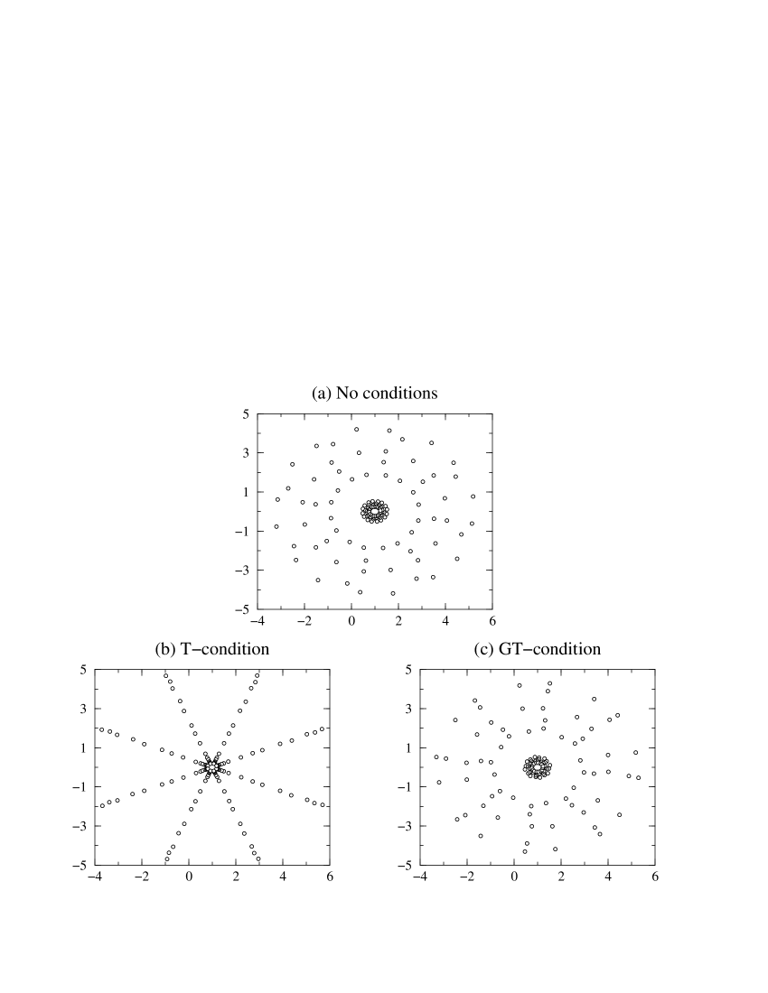
FIG. 5.: The spectrum of $\Lambda(x)$ in the complex plane for a $8\times 8$ lattice in the case of (a) no conditions, (b) the T- and (c) the GT-condition, respectively.

Next, we show that our fermion determinant is positive when all link variables are set unity. In this case $S_{0}^{\dagger}U_{E}$ can be easily diagonalized in the momentum space. The eigenvalues are expressed by the eigenvalues ${\lambda_{U}}_{m}$ of $U_{E}$ as

$${\lambda_{U}}_{m}\exp\left(i\frac{2n+1}{N_{T}}\pi\right)\qquad(n=0,\ldots,N_{T}-1).$$ (57)

Therefore

$$\det\Lambda=\prod_{m,n}\left(1-{\lambda_{U}}_{m}\exp\left(i\frac{2n+1}{N_{T}}\pi\right)\right)$$ (58)

is clearly positive, as ${\lambda_{U}}_{m}$ can be shown positive.

The configuration with all link variables unity clearly satisfies the T- and the GT-condition. This seems to complete our proof for the positivity of the determinant. It should be noticed that we might be faced with configurations where some $\lambda$ with $\left|\lambda\right|=1$ is not degenerated in spite of the symmetry $\lambda$ and ${\lambda^{\ast}}^{-1}$. In this case the relation Eq.(56) does not hold and our proof fails. However, such configurations are very hard to happen.

C SU(N) gauge group

When the gauge group is SU(N), we can also make similar discussion to the U(1) gauge group case and find the positivity of our fermion determinant. In this case, from Eq.(35) we immediately see

$$\det Q({\mbox{\boldmath$x$}}) = \pm\left|U_{(1,{\mbox{\boldmath$x$}}),(2,{\mbox{\boldmath$x$}})}\right|\left|U_{(2,{\mbox{\boldmath$x$}}),(3,{\mbox{\boldmath$x$}})}\right|\ldots\left|U_{(N_{T}-1,{\mbox{\boldmath$x$}}),(0,{\mbox{\boldmath$x$}})}\right|$$ (59)

$$= \pm 1,$$ (60)

so we find $\det S_{0}(x)=1$ without any conditions. Consequently, the determinant of our fermion matrix is always real in the case of SU(N) gauge fields. And we find that our fermion determinant is positive in the $(1+1)$-dimensional SU(N), since the two symmetries of the spectrum of $\Lambda(x)$ discussed above are also satisfied. In fact we can confirm the symmetries from the spectra shown in Figs.6(a) and 6(b) for SU(2) and SU(3), respectively. And, in Figs.7(a) and 7(b), we display the numerical results for the distribution of our fermion determinant in the $(1+1)$-dimensional SU(2) and SU(3) gauge theories. The results show that fermion determinants are real and positive in both cases.

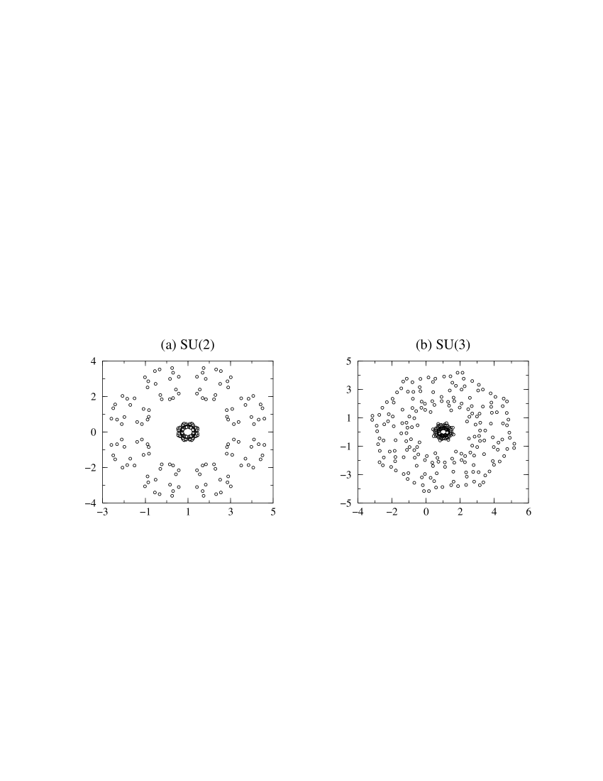
FIG. 6.: The spectrum of $\Lambda(x)$ in the complex plane for a $8\times 8$ lattice. Plots (a) and (b) correspond to SU(2) and SU(3) gauge groups, respectively.

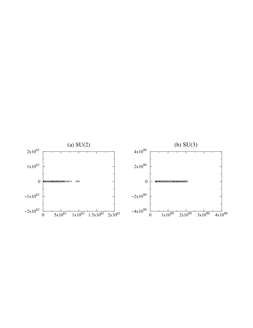
FIG. 7.: The distributions of our fermion determinant in the complex plane for each configuration of 2000 Monte Carlo iterations on a $8\times 8$ lattice at $\beta=2.0$. Plots (a) and (b) correspond to SU(2) and SU(3) gauge groups, respectively.

We conclude that our fermion determinant $\det\Lambda(x)$ in (1+1)-dimensions is real and positive for U(1) gauge group under the T- or the GT-condition and for SU(N) gauge group without any conditions, though we have only a plausible reason for the positivity.

IV Discussion and summary

When we applied our new action without any conditions to U(1) gauge theory on a lattice, we were faced with the problem of convergence in Monte Carlo simulation. In this note, we showed that we could avoid this problem by imposing the T- or the GT-condition. In order to make this situation clear, as an example, we study the propagator of the fermi field,

$$\langle\psi(y)\psi^{\dagger}(y^{\prime})\rangle=\frac{\displaystyle{\int d\psi d\psi^{\dagger}dU\psi(y)\psi^{\dagger}(y^{\prime})e^{-S_{g}-S_{f}}}}{\displaystyle{\int d\psi d\psi^{\dagger}dUe^{-S_{g}-S_{f}}}}.$$ (61)

Integrating in Eq.(61) with respect to $\psi(x)$ and $\psi^{\dagger}(x)$ we have

$$\langle\psi(y)\psi^{\dagger}(y^{\prime})\rangle=\frac{\displaystyle{\int dU\det\left(1-S_{0}^{\dagger}(x)U_{E}(x)\right)\left(1-S_{0}^{\dagger}(x)U_{E}(x)\right)_{y,y^{\prime}}^{-1}e^{-S_{g}}}}{\displaystyle{\int dU\det\left(1-S_{0}^{\dagger}(x)U_{E}(x)\right)e^{-S_{g}}}}.$$ (62)

We introduce new variables $\Theta$ and $\tilde{\theta}_{0}(x)$ instead of link variables $U_{x,x+\hat{0}}=e^{i\theta_{0}(x)}$,

$$\theta_{0}(x)=\Theta+\tilde{\theta}_{0}(x),$$ (63)

and using the following equation

$$\int\prod_{x}d\tilde{\theta}_{0}(x)d\Theta\delta\left(\sum_{x}\tilde{\theta}_{0}(x)\right)$$

$$\;\;\;=\int\prod_{x}d\theta_{0}(x)d\Theta\delta\left(\sum_{x}\theta_{0}(x)-N_{T}N_{X}\Theta\right)$$

$$\;\;\;=\frac{1}{N_{T}N_{X}}\int\prod_{x}d\theta_{0}(x),$$

we get

$$\langle\psi(y)\psi^{\dagger}(y^{\prime})\rangle$$ (64)

$$\;\;\;=\frac{\displaystyle{\int d\tilde{U}d\Theta\delta\left(\sum_{x}\tilde{\theta}_{0}(x)\right)\det\left(1-e^{i\Theta}{\tilde{S}_{0}(x)}^{\dagger}U_{E}(x)\right)\left(1-e^{i\Theta}{\tilde{S}_{0}(x)}^{\dagger}U_{E}(x)\right)_{y,y^{\prime}}^{-1}e^{-\tilde{S}_{g}}}}{\displaystyle{\int d\tilde{U}d\Theta\delta\left(\sum_{x}\tilde{\theta}_{0}(x)\right)\det\left(1-e^{i\Theta}{\tilde{S}_{0}(x)}^{\dagger}U_{E}(x)\right)e^{-\tilde{S}_{g}}}},$$ (65)

where the tilde represents replacing $\theta_{0}(x)$ by $\tilde{\theta}_{0}(x)$.

The phase of determinant $\det(1-e^{i\Theta}{\tilde{S}_{0}(x)}^{\dagger}U_{E}(x))$ takes any value between $0$ and $2\pi$ as is shown in Fig.1(a). The summation of $\det(1-e^{i\Theta_{n}}{\tilde{S}_{0}(x)}^{\dagger}U_{E}(x))$ over a sequence $\Theta_{n}(n=1,2,\ldots)$ which is chosen at random are canceled out accidentally, then the denominator of Eq.(65) becomes very small. This is the origin of unstable behavior in Monte Carlo simulation. Indeed in Sec.3, under the T- or the GT-condition which ensures that the variable $\Theta$ is fixed zero, we proved the determinant $\det(1-S_{0}^{\dagger}(x)U_{E}(x))$ in the $(1+1)$-dimensional lattice to be real for all configurations of link variables and to be positive for most ones.

We have another reason for fixing $\Theta$, namely, imposing some condition like the T- or the GT-condition. Since the integrand of the numerator in Eq.(65) is equal to the cofactor of matrix $(1-e^{i\Theta}{\tilde{S}_{0}(x)}^{\dagger}U_{E}(x))$ whose elements are linear functions of $e^{i\Theta}$, it is a polynomial of $e^{i\Theta}$. After we integrate it with respect to $\Theta$, all terms of this polynomial vanish besides constant terms. For the denominator of Eq.(65) we can say the same thing as the above, thus we have

$$\langle\psi(y)\psi^{\dagger}(y^{\prime})\rangle=\mbox{\bf{1}}_{y,y^{\prime}},$$ (66)

which is an undesired result. Contrarily, if we choose some condition, like the T- or the GT-condition, we may avoid this trouble.

When we try applying this fermion to the SU(N) lattice gauge theory, we can expect that there is no necessity for imposing some condition because the element like $e^{i\Theta}$ does not belong to the group SU(N). In fact, it is shown that the fermion determinant is real for all configurations and that it is positive for most configurations. And the numerical simulation for SU(2) and SU(3) gauge theory shows that the fermion determinants are real and positive. We will discuss the application of our fermions to SU(N) lattice gauge theory in higher dimensions elsewhere.

REFERENCES

- [1] H. B. Nielsen and M. Ninomiya, Nucl. Phys. B185, 20 (1981); B193, 173 (1981).
- [2] K. Wilson, Phys. Rev. D 10, 2445 (1974); New Phenomena in Subnuclear Physics, edited by A. Zichichi (Plenum, New York, 1977).
- [3] L. Susskind, Phys. Rev. D 16, 3031 (1977).
- [4] P. H. Ginsparg and K. G. Wilson, Phys. Rev. D 25, 2649 (1982).
- [5] F. Niedermayer, Nucl. Phys. Proc. Suppl. 73, 105 (1999) and references therein.
- [6] I. Horváth, Phys. Rev. Lett. 81, 4063 (1998); W. Bietenholz, hep-lat/9901005.
- [7] A. Hayashi, T. Hashimoto, M. Horibe, and H. Yamamoto, Phys. Rev. D 55, 2987 (1997).
- [8] M. Horibe, T. Hashimoto, A. Hayashi, and H. Yamamoto, Phys. Rev. D 56, 6006 (1997).
- [9] H. J. Rothe, LATTICE GAUGE THEORIES -AN INTRODUCTION- (World Scientific, Singapore, 1992).