Large-$q$ expansion for the second moment correlation length in the two-dimensional $q$-state Potts model

Abstract

We calculate the large-$q$ expansion of the second moment correlation length at the first order phase transition point of the $q$-state Potts model in two dimensions both in the ordered and disordered phases to order 21 in $1/\sqrt{q}$. They coincide with each other to the third term of the series but differ a little in higher orders. Numerically the ratio of the second moment correlation length in the two phases is not far from unity in all region of $q>4$. The ratio of the second moment correlation length to the standard correlation length in the disordered phase is far from unity, which suggests that the second largest and smaller eigenvalues of the transfer matrix form a continuum spectrum not only in the large-$q$ region but also in all the region of $q>4$.

1 Introdunction

The $q$-state Potts model[1, 2] in two dimensions exhibits the first order phase transition for $q>4$. Many quantities[3] was solved exactly at the phase transition point, among which the correlation length $\xi^{(d)}$ in the disordered phase [4, 5, 6] is included. On the other hand, no analytic result had been known for the correlation length $\xi^{(o)}$ in the ordered phase at the phase transition point. Here the correlation length means the standard one defined from the ratio of the largest to the second largest eigenvalues of the transfer matrix and it is often called the true correlation length or the exponential correlation length. Janke and Kappler[7] examined the decay rate of the correlation function by the Monte Carlo simulation with large sizes of the lattice for $q=10,15$ and $20$ giving a result that was consistent with $\xi^{(o)}=\xi^{(d)}$ and they made a conjecture that this relation would be exact. Iglói and Carlon[8] evaluated the largest and the second largest eigenvalues of the transfer matrix for $q=9$ by the density matrix renormalization group technique with a result that supports this conjecture. Recently the author[9] investigated analytically the large-$q$ behavior of the eigenvalues of the transfer matrix. He found that from the second largest to the $L$-th largest eigenvalues with $L$ the size of the lattice make a continuum spectrum for the thermodynamic limit both in the ordered and disordered phases at least in the large-$q$ region and that $\xi^{(o)}=\xi^{(d)}$ at least to order $z^{3/2}$ (i.e., in the first 4 terms of the large-$q$ expansion).

Here we calculate the large-$q$ expansion of the second moment correlation length $\xi_{2nd}$ at the first order phase transition point both in the ordered and disordered phases of this model. The second moment correlation length also gives important informations on the spectrum of the eigenvalues of the transfer matrix. The large-$q$ expansion of the Potts model in two dimensions was calculated to order $z^{10}$ ($z\equiv 1/\sqrt{q}$) for the energy cumulants including the specific heat by Bhattacharya, Lacaze and Morel[10] using a graphical method. Tabata and the author[11, 12] extended the large-$q$ series to order $z^{23}$ using the finite lattice method[13, 14, 15]. They also calculated the large-$q$ series for the magnetization cumulants including the magnetic susceptibility to order $z^{21}$. These long series enabled them to present the estimate for the numerical values of the cumulants which is orders of magnitude more precise than that of Monte Carlo simulations. The series also served to convince us that the correctness of the conjecture by Bhattacharya, Lacaze and Morel on the behavior of the divergent quantities in the limit of $q\to 4$. It is rather straightforward to apply the finite lattice method to the large-$q$ expansion of the second moment correlation length, since the algorithm is quite parallel with that of the finite lattice method for the low temperature expansion of the second moment correlation length for the Ising model in three dimensions[17]. The situation is in contrast to the case of the standard correlation length where the continuum spectrum of the eigenvalues of the transfer matrix prevented us from applying the method used to obtain the low temperature series for the Ising model in three dimensions[18, 19]. The results of the large-$q$ expansion for the second moment correlation length was reported breafly in reference[9] and here we describe them in detail.

2 Expansion series by the finite lattice method

The model is defined on the $L_{x}\times L_{y}$ rectangular lattice by the partition function

$$Z=\sum_{\{s_{i}\}}\exp{\left\{\beta\sum_{\langle i,j\rangle}\delta_{s_{i},s_{j}}+\sum_{i}(h+\gamma_{1}x_{i}+\gamma_{2}y_{i}+\eta\mbox{\boldmath$r$}_{i}^{2})\delta_{s_{i},1}\right\}}\;,$$ (1)

where the spin variable $s_{i}$ at each site $i$ takes the values $1,2,\cdots,q$, $\langle i,j\rangle$ represents the pair of nearest neighbor sites and $\mbox{\boldmath$r$}_{i}=(x_{i},y_{i})$ is the coordinate of the site $i$. The phase transition point $\beta_{t}$ for $h=\gamma_{1}=\gamma_{2}=\eta=0$ is given by $\exp{(\beta_{t})-1=\sqrt{q}}$. The fixed boundary condition should be taken for the ordered phase in which all the spins outside the $L_{x}\times L_{y}$ lattice are fixed to be $\{s_{i}=+1\}$, and the free boundary condition should be taken for the disordered phase.

The second moment correlation length squared is defined by

$$\xi_{2nd}^{2}=\frac{\mu_{2}}{2d\mu_{0}},$$ (2)

where $\mu_{2}$ is the second moment of the correlation function

$$\mu_{2}=\lim_{L_{x},L_{y}\rightarrow\infty}(L_{x}L_{y})^{-1}\sum_{i,j}(\mbox{\boldmath$r$}_{i}-\mbox{\boldmath$r$}_{j})^{2}\langle\delta_{s_{i},1}\delta_{s_{j},1}\rangle_{c},$$ (3)

$\mu_{0}$ is the zeroth moment of the correlation function, i.e., the magnetic susceptibility, and $d(=2)$ is the dimensionality of the lattice. The second moment $\mu_{2}$ can be obtained by the derivative of the free energy density as

$$\mu_{2} = \lim_{L_{x},L_{y}\rightarrow\infty}(L_{x}L_{y})^{-1}$$ (4)

$$\times\left.2\left(\frac{\partial^{2}}{\partial h\partial\eta}-\frac{\partial^{2}}{\partial\gamma_{1}^{2}}-\frac{\partial^{2}}{\partial\gamma_{2}^{2}}\right)\ln{Z(\beta,h,\eta,\gamma_{1},\gamma_{2})}\right|_{h=\eta=\gamma_{1}=\gamma_{2}=0}.$$

The algorithm of the finite lattice method to generate the large-$q$ expansion series for the second moment $\mu_{2}$ is the following. We define $H(l_{x},l_{y})$ for each $l_{x}\times l_{y}$ lattice ($1\leq l_{x}\leq L_{x},1\leq l_{y}\leq L_{y}$) as

$$\!\!\!\!\!\!\!\!\!\!\!\!\!H(l_{x},l_{y})=\left.2\left(\frac{\partial^{2}}{\partial h\partial\eta}-\frac{\partial^{2}}{\partial\gamma_{1}^{2}}-\frac{\partial^{2}}{\partial\gamma_{2}^{2}}\right)\ln{Z(l_{x},l_{y})}\right|_{h=\eta=\gamma_{1}=\gamma_{2}=0},$$ (5)

where $Z(l_{x},l_{y})$ is the partition function for the $l_{x}\times l_{y}$ lattice with the fixed and free boundary condition for the ordered and disordered phase, respectively, and define $W$ of each lattice recursively as

$$W(l_{x},l_{y}) = H(l_{x},l_{y})$$ (6)

$$-\sum_{\scriptstyle 1\leq l_{x}^{\prime}\leq l_{x},1\leq l_{y}^{\prime}\leq l_{y}\atop\scriptstyle(l_{x}^{\prime},l_{y}^{\prime})\neq(l_{x},l_{y})}(l_{x}-l_{x}^{\prime}+1)(l_{y}-l_{y}^{\prime}+1)W(l_{x}^{\prime},l_{y}^{\prime})\;.$$

Note that $H(l_{x},l_{y})$ and $W(l_{x},l_{y})$ depend on the size $l_{x}$ and $l_{y}$ but not on the position of the origin of the coordinate. Then the second moment of the correlation function in the thermodynamic limit is given by

$$\mu_{2}=\sum_{l_{x},l_{y}}W(l_{x},l_{y}).$$ (7)

We can prove[15] that the Taylor expansion of $W(l_{x},l_{y})$ with respect to $z\equiv 1/\sqrt{q}$ includes the contribution from all the clusters of polymers in the standard cluster expansion[16] that can be embedded into the $l_{x}\times l_{y}$ lattice but cannot be embedded into any of its rectangular $l_{x}^{\prime}\times l_{y}^{\prime}$ sub-lattices with $l_{x}^{\prime}\leq l_{x},l_{y}^{\prime}\leq l_{y}$. It is straightforward to understand from the discussion for the large-$q$ expansion of the magnetic susceptibility in reference[12] that the series expansion of $W(l_{x},l_{y})$ starts from the order of $z^{n}$ with $n=l_{x}+l_{y}$ in the ordered phase and $n=l_{x}+l_{y}-2$ in the disordered phase, respectively. So in order to obtain the expansion series to order $z^{N}$, we should take all the finite-size rectangular lattices for the summation in equation (7) that satisfy $l_{x}+l_{y}\leq N$ in the ordered phase and $l_{x}+l_{y}-2\leq N$ in the disordered phase, respectively.

Using these algorithm of the finite lattice method we have calculated the series for the second moment $\mu_{2}$ at the first order phase transition point to order $N=21$ in $z$ both in the ordered and disordered phases as

$$\mu_{2}=\sum_{n}a_{n}z^{n}.$$ (8)

The coefficients of the series are listed in table 1. We have checked that all of $W(l_{x},l_{y})$ with $l_{x}+l_{y}-2\leq N$ for the ordered phase and with $l_{x}+l_{y}\leq N$ for the disordered phase have the correct order in $z$ as described above.

Table 1: The large-$q$ expansion coefficients $a_{n}$ for the second moment $\mu_{2}$ of the correlation function at $\beta=\beta_{t}$ in the ordered and disordered phases.

$n$	$a_{n}$(ordered)	$a_{n}$(disordered)
$0$	$0$	$0$
$1$	$0$	$0$
$2$	$0$	$0$
$3$	$4$	$4$
$4$	$44$	$44$
$5$	$344$	$336$
$6$	$2140$	$2064$
$7$	$11676$	$11164$
$8$	$57440$	$54652$
$9$	$261884$	$248456$
$10$	$1121092$	$1062320$
$11$	$4560648$	$4320948$
$12$	$17761800$	$16840044$
$13$	$66657396$	$63279396$
$14$	$242180712$	$230307200$
$15$	$855255360$	$815001104$
$16$	$2945011236$	$2812875600$
$17$	$9914462596$	$9493154576$
$18$	$32704960680$	$31397031360$
$19$	$105910040516$	$101949411404$
$20$	$337252952816$	$325538033480$
$21$	$1057475140292$	$1023600956088$

Combining with the large-$q$ series of the magnetic susceptibility given in reference[12], we obtain the series for the second moment correlation length squared $\xi_{2nd}^{2}$ as

$$\xi_{2nd}^{2}=\sum_{n}b_{n}z^{n},$$ (9)

which are listed in table 2. The obtained expansion coefficients for the ordered and disordered phases coincide with each other to order $z^{3}$ and differ a bit from each other in higher orders.

Table 2: The large-$q$ expansion coefficients $b_{n}$ for the second-moment correlation length squared $\xi_{2nd}^{2}$ at $\beta=\beta_{t}$ in the ordered and disordered phases.

$n$	$b_{n}$(ordered)	$b_{n}$(disordered)
$0$	$0$	$0$
$1$	$1$	$1$
$2$	$7$	$7$
$3$	$35$	$35$
$4$	$154$	$157$
$5$	$611$	$635$
$6$	$2237$	$2363$
$7$	$7720$	$8271$
$8$	$25461$	$27569$
$9$	$80852$	$88271$
$10$	$249212$	$273775$
$11$	$748239$	$825956$
$12$	$2198991$	$2436937$
$13$	$6335396$	$7044039$
$14$	$17961597$	$20027792$
$15$	$50129172$	$56038776$
$16$	$138121342$	$154746684$
$17$	$375778895$	$421876179$
$18$	$1011869143$	$1137902174$
$19$	$2695052762$	$3035669883$

3 Analysis of the series

It is known[20] that in the limit of the large correlation length

$$\frac{\xi_{2nd}^{2}}{\xi_{1}^{2}}\to\frac{\sum_{j=1}^{\infty}c_{j}^{2}(\xi_{j}/\xi_{1})^{3}}{\sum_{j=1}^{\infty}c_{j}^{2}(\xi_{j}/\xi_{1})}$$ (10)

with $\xi_{j}\equiv-\ln{(\Lambda_{j}/\Lambda_{0})}$ and $c_{j}=<\Lambda_{0}|{\cal O}|\Lambda_{j}>$ where $\Lambda_{j}(j=0,1,2,\cdots)$ are the eigenvalues of the transfer matrix with $\Lambda_{0}$ the largest one, $|\Lambda_{j}>$ is the eigenstate of the transfer matrix corresponding to the eigenvalue $\Lambda_{j}$ and ${\cal O}=\sum_{i}\delta_{s_{i},1}$ with the summation for $i$ running over the sites with a fixed coordinate of $y_{i}$. The $\xi_{1}\equiv-\ln{(\Lambda_{1}/\Lambda_{0})}$ is the standard correlation length. Later on we will call the eigenstate $\Lambda_{1}$ the first excited state and $\Lambda_{j}$($i=2,3,\cdots$) the higher excited states.

The standard correlation length $\xi_{1}^{(d)}$ at the phase transition point in the disordered phase is known exactly with its asymptotic behavior for $q\to 4$ as

$$\xi_{1}^{(d)}\sim\frac{1}{8\sqrt{2}}\exp{\left(\frac{\pi^{2}}{2\theta}\right)},$$ (11)

where $2\cosh{\theta}=\sqrt{q}$ ($\theta\sim\sqrt{q-4}/2$ for $q\to 4$). It is quite natural to expect that all of the $\xi_{j}$’s behave like

$$\xi_{j}^{(o,d)}\sim C_{j}^{(o,d)}\exp{\left(\frac{\pi^{2}}{2\theta}\right)}$$ (12)

for $q\to 4$ both in the ordered and disordered phases, in which case

$$\xi_{2nd}^{(o,d){}^{2}}\sim A^{(o,d)}\exp{\left(\frac{\pi^{2}}{\theta}\right)}.$$ (13)

To check the validity of this conjecture we follow the method in reference[11, 12] adopted to analyze the large-$q$ series of the energy and magnetization cumulants including the specific heat and the magnetic susceptibility. The method was used to convince the validity of the Bhattacharya-Lacaze-Morel conjecture on the asymptotic behavior of these quantities for $q\to 4$. The latent heat ${\cal L}$ is known exactly with the asymptotic form for $q\to 4$ as[21]

$${\cal L}\sim 3\pi\exp{\left(-\frac{\pi^{2}}{4\theta}\right)}\;,$$ (14)

so, if $\xi_{2nd}^{(o,d)}{}^{2}$ has the asymptotic form in equation (13), the product $\xi_{2nd}^{2}{\cal L}^{p}$ is a smooth function of $z$ for $q\to 4$ when $p=4$, and the Padé approximants of the large-$q$ series for this product are expected to converge for $p=4$. The results are given in figure 1. We can see that the convergence is really good around $p=4$ both in the ordered and disordered phases.

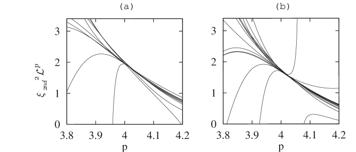
Figure 1: The Padé approximants of the second moment correlation length squared multiplied by the $p$-th power of the latent heat (a) in the disordered phase and (b) in the ordered phase.

The estimated values of the second moment correlation length by setting $p=4$ are listed in table.3. We note that the ratio of the estimated values of the second moment correlation length in the ordered to disordered phases $\xi_{2nd}(\mbox{ordered})/\xi_{2nd}(\mbox{disordered})$ is not far from unity. The ratio is 0.935(5) even for $q\to 4$.

Table 3: Estimates of the second moment correlation length $\xi_{2nd}$ for each $q$ in the ordered and disordered phases.

$q$	$\xi_{2nd}$(ordered)	$\xi_{2nd}$(disordered)
5	1261(4)	1349(6)
6	83.1(1)	88.5(1)
7	25.89(1)	27.45(2)
8	13.140(2)	13.855(5)
9	8.3440(5)	8.751(4)
10	5.9965(2)	6.260(1)
12	3.79944(3)	3.9355(1)
15	2.480927(4)	2.54815(1)
20	1.6376632(4)	1.667680(1)
30	1.0633984(1)	1.0742339(1)

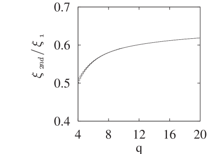
Figure 2: The ratio $\xi_{2nd}/\xi_{1}$ of the second moment correlation length to the standard correlation length in the disordered phase.

Another interesting and important quantity is the ratio of the second moment correlation length $\xi_{2nd}$ to the standard correlation length $\xi_{1}$. From equation (10) we know that the ratio $\xi_{2nd}/\xi_{1}$ should be less than unity in the limit of the large correlation length. If the higher excited states ($i=2,3,\cdots$) did not contribute so much, this ratio would be close to unity, as is the case in the Ising model on the simple cubic lattice, where $\xi_{2nd}/\xi_{1}=0.970(5)$ at the critical point in the disordered phase [20, 22].

In figure 2 we plot the ratio $\xi_{2nd}/\xi_{1}$ for the Potts model in the disordered phase. We use the value of $\xi_{2nd}$ estimated above from the Padé analysis of $\xi_{2nd}^{2}{\cal L}^{4}$ and the exact value of $\xi_{1}$. The ratio is much less than unity in the region of $q$ where the correlation length is large enough. It approaches $0.505(6)$ for $q\to 4$. This result implies that the contribution of the higher excited states is important in the Potts model in two dimensions. It is consistent with the fact that the eigenvalue of the transfer matrix for the first excited state locates at the edge of the continuum spectrum of the eigenvalues of the transfer matrix at least in the large-$q$ region and it strongly suggests that these excited states ($i=1,2,\cdots,L_{x}$) form a continuum spectrum not only in the large-$q$ region but also even in the limit of $q\to 4$.

4 Summary

We calculated the large-$q$ expansion of the second moment correlation length in the ordered and disordered phases of the $q$-state Potts model in two dimensions and found that they coincide with each other to the third term of the expansion but differ a little from each other in higher orders. This suggests that, although the first few terms of the large-$q$ expansion for the standard correlation length really coincide in the ordered and disordered phases, their higher order terms might be different from each other. Note, however, that it is not conclusive, since the second moment correlation length depends not only on the spectrum of the eigenvalues of the transfer matrix but also on the overlapping amplitude $c_{i}$ which appeared in equation (10). Numerically the ratio $\xi_{2nd}^{(o)}/\xi_{2nd}^{(d)}$ is not far from unity even in the limit of $q\to 4$. We also found that $\xi_{2nd}^{(d)}/\xi_{1}^{(d)}$ is far from unity for all region of $q>4$. It implies that higher excited states give significant contributions as well as the first excited state and it strongly suggests that these excited states form a continuum spectrum (i.e., there is no particle state in the language of the field theory) not only in the large-$q$ region but also in all the region of $q>4$. Finally we point out that it is worthwhile to reanalyze the previous Monte Carlo data for the correlation function on the assumption that this would be the case.

References

- [1] Potts R B 1952 Proc. Camb. Phil. Soc. 48 106
- [2] Wu F Y 1982 Rev. Mod. Phys. 54 235
- [3] Baxter R J 1973 J. Phys. C 6 L445; 1973 J. Stat. Phys. 9 145
- [4] Klümper A, Schadschneider A and Zittartz J 1989 Z. Phys. B 76 247
- [5] Buffenoir E and Wallon S 1993 J. Phys. A 26 3045
- [6] Borgs C and Janke W 1992 J. Phys. I (France) 2 649
- [7] Janke W and Kappler S 1994 Nucl. Phys. B (Proc. Suppl.) 34 1155
- [8] Iglói F and Carlon E 1999 Phys. Rev. B 59 3783
- [9] Arisue H 1999 hep-lat/9909166 to appear in Proceedings of the International Synposium on Lattice Field Theory(1999 Pisa)
- [10] Bhattacharya T, Lacaze R and Morel A 1997 J. Phys. I (France) 7 1155
- [11] Arisue H and Tabata K 1999 Phys. Rev. E 59 186
- [12] Arisue H and Tabata K 1999 Nucl. Phys. B 546[FS] 558
- [13] de Neef T and Enting I G 1977 J. Phys. A 10 801; Enting I G 1978 J. Phys. A 11 563; 1996 Nucl. Phys. B (Proc. Suppl.) 47 180
- [14] Creutz M 1991 Phys. Rev. B 43 10659
- [15] Arisue H and Fujiwara T 1984 Prog. Theor. Phys. 72 1176; Arisue H 1994 Nucl. Phys. B (Proc. Suppl.) 34 240
- [16] Münster G 1981 Nucl. Phys. B 180[FS2] 23
- [17] Arisue H and Tabata K 1995 Nucl. Phys. B 435[FS] 555
- [18] Arisue H and Fujiwara T 1987 Nucl. Phys. B 285[FS] 253
- [19] Arisue H and Tabata K 1994 Phys. Letters B 322 224
- [20] Caselle M, Hasenbusch M and Provero P 1999 hep-lat/9903011
- [21] Bhattacharya T, Lacaze R and Morel A 1995 Nucl. Phys. B 435 526
- [22] Campostrini M, Pelissetto A, Rosi P and Vicari E 1998 Phys. Rev. E 57 184