The Photon Structure from Deep Inelastic Electron-Photon Scattering

Abstract

The present knowledge of the structure of the photon is presented with emphasis on measurements of the photon structure obtained from deep inelastic electron-photon scattering at $\mathrm{e^{+}}\,\mathrm{e^{-}}$ colliders. This review covers the leptonic and hadronic structure of quasi-real and also of highly virtual photons, based on measurements of structure functions and differential cross-sections. Future prospects of the investigation of the photon structure in view of the ongoing LEP2 programme and of a possible linear collider are addressed. The most relevant results in the context of measurements of the photon structure from photon-photon scattering at LEP and from photon-proton and electron-proton scattering at HERA are summarised.

Ginwidth=0.95

1 Introduction

The photon is a fundamental ingredient of our present understanding of the interactions of quarks and leptons. These interactions are successfully described in the framework of the standard model, a theory which consists of a combination of gauge theories. Being the gauge boson of the theory of Quantum Electro Dynamics, QED, the photon mediates the electromagnetic force between charged objects. In these interactions the photon can be regarded as a structureless object, called the direct, or the bare photon. Since QED is an abelian gauge theory, the photon has no self-couplings and to the best of our knowledge the photon is a massless particle.

Due to the Heisenberg uncertainty principle, written as $\Delta E\Delta t>1$, the photon, denoted with $\gamma$, is allowed to violate the rule of conservation of energy by an amount of energy $\Delta E$ for a short period of time $\Delta t$ and to fluctuate into a charged fermion anti-fermion, $\mathrm{f\bar{f}}$, system carrying the same quantum numbers as the photon, $\gamma\rightarrow\mathrm{f\bar{f}}\rightarrow\gamma$. If, during such a fluctuation, one of the fermions interacts via a gauge boson with another object, then the parton content of the photon is resolved and the photon reveals its structure. In such interactions the photon can be regarded as an extended object consisting of charged fermions and also gluons, the so called resolved photon. This possibility for the photon to interact either directly or in a resolved manner is another dual nature of the photon, which is the cause of a variety of phenomena and makes the photon a very interesting object to investigate. One possible description of the structure of the photon is given by the concept of photon structure functions, which is the main subject of this review.

Today the main results on the structure of the photon are obtained from the electron-positron collider LEP and the electron-proton collider HERA. The largest part of this review is devoted to the discussion of deep inelastic electron-photon scattering and to the measurements of QED and hadronic structure functions of the photon. Other LEP results on the structure of the photon apart from those obtained from deep inelastic electron-photon scattering, as well as the measurements in photoproduction and deep inelastic electron-proton scattering at HERA, are summarised briefly.

The review is organised in the following way. In Section 2.1 the kinematical quantities are introduced and in Section 2.2 the capabilities of the detectors to measure the deep inelastic electron-photon scattering process are discussed. The theoretical formalism needed to measure the photon structure is outlined in Section 3, with special emphasis on the QED and hadronic structure functions of the photon in Section 3.3 and Section 3.4 respectively. A review of the available parametrisations of parton distribution functions of the photon is given in Section 4. The most important tools used to measure the photon structure are described in Section 5, concentrating on event generators and unfolding methods. The measurements of the QED and hadronic structure of the photon obtained from leptonic and hadronic final states are discussed in Section 6, and Section 7 respectively. The prospects of future determinations of the structure of the photon are outlined. The measurements expected to be performed at LEP, using the high statistics, high energy data still expected within the ongoing LEP2 programme, are discussed in Section 8.1, followed by the discussion of measurements to be performed at a possible future linear collider in Section 8.2. Complementary investigations of the photon structure from LEP and selected HERA results are addressed in Section 9.

Additional information is presented in the appendices. The relation between the cross-section picture and the structure function picture is outlined in Appendix A, followed by a discussion of the general relation between the photon structure function, the parton distribution functions and the evolution equations given in Appendix B. The Appendices C and D contain a collection of numerical results on measurements of the photon structure.

1.1 Theoretical description of photon interactions

In deep inelastic electron-photon scattering the structure of a quasi-real photon, $\gamma$, is probed by a highly virtual photon, $\gamma^{\star}$, emitted by a deeply inelastically scattered electron, as sketched in Figure 1.

Figure 1: Probing the structure of quasi-real photons, $\gamma$, by highly virtual photons, $\gamma^{\star}$.

The photon, as the mediator of the electromagnetic force, couples to charged objects. The fundamental coupling of the photon as described in the framework of QED is the coupling to charged fermions, $\rm f$, which can be either quarks, $\rm q$, or leptons, $\ell$, with $\ell=\rm e\mu\tau$. For the case of lepton pair production, the process can be calculated in QED. The relevant formulae are listed in Section 3 and the results on the QED structure of the photon are discussed in Section 6.

Figure 2: The different appearances of the photon. Shown are (a) the direct or bare photon, and (b,c) the resolved photon, which can be either point-like, (b), or hadron-like, (c).

For the production of quark pairs the situation is more complex, since the spectrum of fluctuations is richer, and QCD corrections have to be taken into account. Therefore, the photon interactions receive several contributions shown in Figure 2. The leading order contributions are discussed in detail. The reactions of the photon are usually classified depending on the object which takes part in the hard interaction. If the photon directly, as a whole, takes part in the hard interaction, as shown in Figure 2(a), then it does not reveal a structure. These reactions are called direct interactions and the photon is named the direct, or the bare photon. If the photon first fluctuates into a hadronic state which subsequently interacts, the processes are called resolved photon processes and structure functions of the photon can be defined. The resolved photon processes are further subdivided into two parts. The first part, shown in Figure 2(b), is perturbatively calculable, as explained in Section 3.4, and called the contribution of the point-like, or the anomalous photon. Here the photon perturbatively splits into a quark pair of a certain relative transverse momentum and subsequently one of the quarks takes part in the hard interaction, which for deep inelastic electron-photon scattering in leading order is the process $\gamma^{\star}\rm q\rightarrow\rm q$. The second part, where the photon fluctuates into a hadronic state with the same quantum numbers as the photon, as shown in Figure 2(c), is usually called the hadron-like, or hadronic contribution. The photon behaves like a hadron, and the hadron-like part of the hadronic photon structure function $F_{2}^{\gamma}$ can successfully be described by the vector meson dominance model, VMD, considering the low mass vector mesons $\rho,\omega$ and $\phi$, as outlined in Section 3.5.

The leading order contributions are subject to QCD corrections due to the coupling of quarks to gluons. The hadronic photon structure function $F_{2}^{\gamma}$ receives contributions both from the point-like part and from the hadron-like part of the photon structure, discussed in detail in Section 3.4.

2 Deep inelastic electron-photon scattering (DIS)

The classical way to investigate the structure of the photon at $\mathrm{e^{+}}\,\mathrm{e^{-}}$ colliders is the measurement of photon structure functions using the process

$$\mathrm{e}{\mathrm{e}}\rightarrow\mathrm{e}{\mathrm{e}}\mathrm{\gamma}^{\star}\,\mathrm{\gamma}\rightarrow\mathrm{e}{\mathrm{e}}X.$$ (1)

In this section the kinematical variables used to describe the reaction are introduced in Section 2.1 and experimental aspects are discussed in Section 2.2.

2.1 Kinematics

Figure 3 shows a diagram of the scattering of two electrons, proceeding via the exchange of two photons of arbitrary virtualities, in the case of leading order fermion pair production, $X=\mathrm{f}\mathrm{f}$.

Figure 3: A diagram of the reaction $\mathrm{e}{\mathrm{e}}\rightarrow\mathrm{e}{\mathrm{e}}\mathrm{f}\mathrm{f}$, proceeding via the exchange of two photons.

The reaction is described in the following notation

$$\mathrm{e}(p_{1})\mathrm{e}(p_{2})\rightarrow\mathrm{e}(p_{1}^{\prime})\mathrm{e}(p_{2}^{\prime})\gamma^{(\star)}(q)\gamma^{(\star)}(p)\rightarrow\mathrm{e}(p_{1}^{\prime})\mathrm{e}(p_{2}^{\prime})\mathrm{f}(p_{\rm f_{1}})\mathrm{f}(p_{\rm f_{2}}).$$ (2)

The terms in brackets denote the four-vectors of the respective particles, and $E$ is the energy of the electrons of the beams. In addition the energies, momentum vectors and polar scattering angles of the outgoing particles are introduced in Figure 3. The symbol $(\star)$ indicates that the photons can be either quasi-real, $\gamma$, or virtual, $\gamma^{\star}$. The virtual photons have negative virtualities $q^{2},p^{2}\leq 0$. For simplicity, the definitions $Q^{2}=-q^{2}\geq 0$ and $P^{2}=-p^{2}\geq 0$ are used, and the particles are ordered such that $Q^{2}>P^{2}$. A list of commonly used variables, which are valid for arbitrary virtualities and for any final state $X$, is given below

$$s_{\rm ee} \equiv (p_{1}+p_{2})^{2}=2p_{1}\cdot p_{2}=4E^{2},$$ (3)

$$s_{\rm e\gamma} \equiv (p_{1}+p)^{2},$$ (4)

$$s_{\gamma\gamma} \equiv W^{2}\equiv(q+p)^{2}=Q^{2}\frac{1-x}{x}-P^{2},$$ (5)

$$x \equiv \frac{Q^{2}}{2p\cdot q}=\frac{Q^{2}}{W^{2}+Q^{2}+P^{2}},$$ (6)

$$y \equiv \frac{p\cdot q}{p_{1}\cdot p},$$ (7)

$$r \equiv \frac{p\cdot q}{p_{2}\cdot q},$$ (8)

$$Q^{2} = xy(s_{\rm e\gamma}+P^{2})=2EE_{1}^{\prime}(1-\cos\theta_{1}^{\prime}),$$ (9)

$$P^{2} = 2EE_{2}^{\prime}(1-\cos\theta_{2}^{\prime}).$$ (10)

Here $s_{\rm ee}$ is the invariant mass squared of the electron-electron system, $s_{\rm e\gamma}$ the invariant mass squared of the electron-photon system, $s_{\gamma\gamma}$ the invariant mass squared of the photon-photon system, and the mass of the electron has been neglected.

Deep inelastic electron-photon scattering is characterised in the limit where one photon is highly virtual, $Q^{2}\gg 0$, and the other is quasi-real, $P^{2}\approx 0$. In this case $P^{2}$ is neglected in the equations above and some simplified expressions are found

$$s_{\rm e\gamma} = (p_{1}+p)^{2}=2p_{1}\cdot p=4EE_{\gamma},$$ (11)

$$y = 1-\frac{E_{1}^{\prime}}{2E}(1+\cos\theta_{1}^{\prime}),$$ (12)

$$r = \frac{E_{\gamma}}{E}\equiv z.$$ (13)

Here $E_{\gamma}$ is the energy of the quasi-real photon.

Figure 4: The different contributions to the reaction $\mathrm{e}{\mathrm{e}}\rightarrow\mathrm{e}{\mathrm{e}}\gamma^{(\star)}\gamma^{(\star)}\rightarrow\mathrm{e}{\mathrm{e}}\mathrm{f}\mathrm{f}$. Shown are (a) the multipheripheral diagram, (b) the t-channel bremsstrahlung diagram and (c) the s-channel bremsstrahlung diagram. In all cases only one possible leading order diagram is shown.

The reaction receives contributions in leading order from the different Feynman diagrams shown in Figure 4. The relative sizes of the contributions of the different Feynman diagrams depend on the kinematical situation. In the region of deep inelastic scattering, $Q^{2}\gg P^{2}\approx 0$, and for moderate values of $Q^{2}$ the dominant contribution stems from the multipheripheral diagram, Figure 4(a). The t-channel bremsstrahlung diagram, Figure 4(b), and the s-channel bremsstrahlung diagram, Figure 4(c), contribute much less to the total cross-section, as explained in Ref. [1]. However, at large values of $Q^{2}$ both bremsstrahlung diagrams have to be taken into account, especially the t-channel bremsstrahlung diagram can be important, predominantly at low invariant masses of the photon-photon system.

The structure functions of the photon, introduced in Sections 3.3 and 3.4, are extracted from a measurement of the differential cross-sections of this reaction. For the measurement of the structure function $F_{2}^{\gamma}$ it is sufficient to describe the reaction in terms of $x$, $Q^{2}$ and $P^{2}$. For the measurement of other structure functions like $F_{\mathrm{A}}^{\gamma}$ and $F_{\mathrm{B}}^{\gamma}$ further variables are necessary. For example, the measurement of $F_{\mathrm{A}}^{\gamma}$ and $F_{\mathrm{B}}^{\gamma}$ in deep inelastic electron-photon scattering involves the measurement of the azimuthal angle $\chi$ between the plane defined by the momentum vectors of the fermion and anti-fermion, called the fermion anti-fermion plane, and the plane defined by the momentum vectors of the incoming and the deeply inelastically scattered electron, called the electron scattering plane.

Figure 5: Illustrations of the scattering angles $\bar{\phi}$, $\theta^{\star}$ and $\chi$ in the photon-photon centre-of-mass system. Shown are (a) the angle between the scattering planes of the two scattered electrons, $\bar{\phi}$, and (b) the scattering angle $\theta^{\star}$ of the fermion or anti-fermion with respect to the photon-photon axis, as well as the the azimuthal angle $\chi$, defined as the angle between the observed electron and the fermion which, in the photon-photon centre-of-mass frame, is scattered at $\cos\theta^{\star}<0$.

The experimentally exploited angles $\bar{\phi}$, $\theta^{\star}$ and $\chi$ are introduced in Figure 5. The azimuthal angle $\bar{\phi}$ is defined as the angle between the scattering planes of the two electrons in the photon-photon centre-of-mass frame, as shown in Figure 5(a). The polar angle $\theta^{\star}$ is defined as the scattering angle of the fermion or anti-fermion with respect to the photon-photon axis in the photon-photon centre-of-mass frame, as shown in Figure 5(b). In this report, the azimuthal angle $\chi$ is defined, as in Ref. [2], as the angle between the observed electron and the fermion which, in the photon-photon centre-of-mass frame, is scattered at $\cos\theta^{\star}<0$, as shown in Figure 5(b). There exist slightly different definitions of $\chi$ in the literature. The different definitions are due to the different choices made to accommodate the fact that the unintegrated structure function $\widetilde{F}_{\mathrm{A}}^{\gamma}$ is antisymmetric in $\cos\theta^{\star}$ if the angle $\chi$ is chosen to be the angle between the electron and the fermion or anti-fermion. There are several ways to redefine $\chi$ in such a way that the integration of $\widetilde{F}_{\mathrm{A}}^{\gamma}$ with respect to $\cos\theta^{\star}$ does not vanish, see Section 3.3 for details.

2.2 Experimental considerations

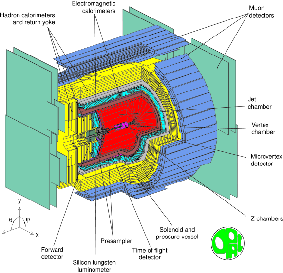
Figure 6: A schematic view of the OPAL detector.

The measurement of structure functions involves the determination of $x$, $Q^{2}$, $P^{2}$ and $\chi$. The capabilities of the different LEP detectors are very similar and they have only slightly different acceptances for the scattered electrons and the final state $X$. As an example, the acceptance of the OPAL detector, shown in Figure 6, is discussed. The scattered electrons are detected by various electromagnetic calorimeters. The final state $X$ is measured with tracking devices and calorimeters which are sensitive to electromagnetic as well as hadronic energy deposits, supplemented by muon detectors. The acceptance ranges of the various components of the OPAL detector are listed in Table 1.

For two values of the energy of the beam electrons $E=45.6$ and 100 $\mathrm{GeV}$ the covered phase space in terms of $x$ and $Q^{2}$, for $P^{2}=0$ is schematically shown in Figure 7. The values of $x$ and $Q^{2}$ are obtained from the kinematical relations listed above, using a range in photon-photon invariant mass of $2.5<W<40/60$ $\mathrm{GeV}$, for $E=45.6/100$ $\mathrm{GeV}$ and assuming that the observed electrons carry at least 50$\%$ of the energy of the beam electrons. The kinematical coverage in principle extends from $10^{-5}$ to about $1$ in $x$ and from $10^{-2}$ to $3\cdot 10^{3}$ $\mathrm{GeV^{2}}$ in $Q^{2}$, but measurements of the photon structure cover only the approximate ranges of $10^{-3}<x<1$ and $1<Q^{2}<10^{3}$ $\mathrm{GeV^{2}}$. This is because at large $Q^{2}$ the statistics are small, and at very low $Q^{2}$ the background conditions are severe.

Table 1: The main parameters of the OPAL detector relevant for measurements of the photon structure. Shown are the acceptance ranges in polar angle $\theta$ for the scattered electrons and the final state $X$. The number 33 mrad reflects the electron acceptance for beam energies within the LEP2 programme, at LEP1 energies the clean acceptance already started at approximately 27 mrad.

scattered electrons
electromagnetic cluster	4-8, 33-55, 60-120, $>200$ [mrad]
final state $X$
charged particles	$|\cos\theta|<0.96$
electromagnetic cluster	$|\cos\theta|<0.98$
hadronic cluster	$|\cos\theta|<0.99$
muons	$|\cos\theta|<0.98$

Therefore the present measurements of the photon structure are limited to $\theta_{1}^{\prime}>33$ mrad, which means $Q^{2}>Q^{2}_{\mathrm{min}}\approx 1.1/5.5$ $\mathrm{GeV^{2}}$, for $E=45.6/100$ $\mathrm{GeV}$, as shown in Figure 7. Here $Q^{2}_{\mathrm{min}}$, calculated from Eq. (9) for $E_{1}^{\prime}=0.5E$ and $\theta_{1}^{\prime}=33$ mrad, is the minimum photon virtuality at which an electron can be observed.

Figure 7: The kinematical coverage of the OPAL detector. Shown are the accepted ranges in $x$ and $Q^{2}$, for $P^{2}=0$ and for two values of the energy of the beam electrons, 45.6 and 100 $\mathrm{GeV}$. The numbers are obtained for specific ranges in $W$ and a minimum energy required for the scattered electron, explained in the text.

The considerations for the $Q^{2}$ acceptance also apply to the acceptance in $P^{2}$ for the second photon. Due to the limited coverage of the detector close to the beam direction the scattered electrons radiating the quasi-real photons cannot be detected up to $\theta_{\rm 2,max}^{\prime}=33$ mrad with the exception of a small region of 4 to 8 mrad. Consequently, for deep inelastic electron-photon scattering the experiments effectively integrate over the invisible part of the $P^{2}$ range up to a value $P^{2}_{\rm{max}}$. Because $P^{2}$ depends on energy and angle of the electron, $P^{2}_{\rm{max}}$ is not a fixed number, but depends on the minimum angle and energy required to observe an electron. Approximations of $P^{2}_{\rm{max}}$ are $Q^{2}_{\mathrm{min}}$ and the $P^{2}$ value corresponding to an electron carrying the energy of the beam electrons and escaping at $\theta_{\rm 2,max}^{\prime}$, which is two times $Q^{2}_{\mathrm{min}}$ in the example from above.

As a consequence of the limited acceptance the measured structure functions depend on the $P^{2}$ distribution of the not observed quasi-real photon, and this dependence increases for increasing energy of the beam electrons.

3 Theoretical framework

In this section the formalism needed for the interpretation of the measurements performed by the various experiments is outlined. The discussion is not complete, but focuses on general considerations and on the formulae relevant for the understanding of the experimental results. These results concern measurements of structure functions and of differential cross-sections, related to the QED and hadronic structure of quasi-real and virtual photons. The structure of quasi-real photons is investigated for $Q^{2}\gg P^{2}\approx 0$, and the structure of virtual photons for the regions $Q^{2},P^{2}\gg m_{\mathrm{e}}^{2}$, or $Q^{2},P^{2}\gg\Lambda^{2}$, where $m_{\mathrm{e}}$ is the mass of the electron and $\Lambda$ is the QCD scale. Since either the cross-section picture, or the structure function picture is relevant for the different measurements, both are discussed in detail, starting with the differential cross-section.

3.1 Individual cross-sections

The general form of the differential cross-section for the scattering of two electrons via the exchange of two photons, Eq. (2), using the multipheripheral diagram integrated over all angles except $\bar{\phi}$ is given as

$$\mathrm{d}^{6}\sigma = \mathrm{d}^{6}\sigma(\mathrm{e}{\mathrm{e}}\rightarrow\mathrm{e}{\mathrm{e}}X)$$ (14)

$$= \frac{\mathrm{d}^{3}p_{1}^{\prime}\mathrm{d}^{3}p_{2}^{\prime}}{E_{1}^{\prime}E_{2}^{\prime}}\frac{\alpha^{2}}{16\pi^{4}Q^{2}P^{2}}\left[\frac{(p\cdot q)^{2}-Q^{2}P^{2}}{(p_{1}\cdot p_{2})^{2}-m_{\mathrm{e}}^{2}m_{\mathrm{e}}^{2}}\right]^{1/2}$$

$$\left(4\rho_{1}^{++}\rho_{2}^{++}\sigma_{\mathrm{TT}}+2|\rho_{1}^{+-}\rho_{2}^{+-}|\tau_{\mathrm{TT}}\cos 2\bar{\phi}+2\rho_{1}^{++}\rho_{2}^{00}\sigma_{\mathrm{TL}}\right.$$

$$\left.+2\rho_{1}^{00}\rho_{2}^{++}\sigma_{\mathrm{LT}}+\rho_{1}^{00}\rho_{2}^{00}\sigma_{\mathrm{LL}}-8|\rho_{1}^{+0}\rho_{2}^{+0}|\tau_{\mathrm{TL}}\cos\bar{\phi}\right)\,,$$

taken from Ref. [4, Eq.5.12]. The four-vectors and kinematic variables are defined in Section 2.1. The total cross-sections $\sigma_{\mathrm{TT}}$, $\sigma_{\mathrm{TL}}$, $\sigma_{\mathrm{LT}}$ and $\sigma_{\mathrm{LL}}$ and the interference terms $\tau_{\mathrm{TT}}$ and $\tau_{\mathrm{TL}}$ correspond to specific helicity states of the photons (T=transverse and L=longitudinal). Since a real photon can have only transverse polarisation, the terms where at least one photon has longitudinal polarisation have to vanish in the corresponding limit $Q^{2}\rightarrow 0$ or $P^{2}\rightarrow 0$. These terms have the following functional form: $\sigma_{\mathrm{LT}}\propto Q^{2}$, $\sigma_{\mathrm{TL}}\propto P^{2}$, $\sigma_{\mathrm{LL}}\propto Q^{2}P^{2}$ and $\tau_{\mathrm{TL}}\propto\sqrt{Q^{2}P^{2}}$. The terms $\rho_{1}^{jk}$ and $\rho_{2}^{jk}$, where $j,k\in(+,-,0)$ denote the photon helicities, are elements of the photon density matrix which depend only on the four-vectors $q$, $p$, $p_{1}$ and $p_{2}$ and on $m_{\mathrm{e}}$. They are taken from Ref. [4, Eq.5.13] and have the following form

$$2\rho_{1}^{++} = \frac{\left(2p_{1}\cdot p-p\cdot q\right)^{2}}{(p\cdot q)^{2}-Q^{2}P^{2}}+1-4\frac{m_{\mathrm{e}}^{2}}{Q^{2}},$$

$$2\rho_{2}^{++} = \frac{\left(2p_{2}\cdot q-p\cdot q\right)^{2}}{(p\cdot q)^{2}-Q^{2}P^{2}}+1-4\frac{m_{\mathrm{e}}^{2}}{P^{2}},$$

$$\rho_{1}^{00} = 2\rho_{1}^{++}-2+4\frac{m_{\mathrm{e}}^{2}}{Q^{2}},$$

$$\rho_{2}^{00} = 2\rho_{2}^{++}-2+4\frac{m_{\mathrm{e}}^{2}}{P^{2}},$$

$$|\rho_{\rm i}^{+-}| = \rho_{\rm i}^{++}-1,$$

$$|\rho_{\rm i}^{+0}| = \sqrt{\left(\rho_{\rm i}^{00}+1\right)|\rho_{\rm i}^{+-}|}.$$ (15)

Experimentally two kinematical limits are studied for leptonic and hadronic final states. Firstly the situation where both photons are highly virtual and secondly the situation where one photon is quasi-real and the other highly virtual: the situation of deep inelastic electron-photon scattering. The corresponding limits of Eq. (14) are discussed next.

If both photons are highly virtual the differential cross-section reduces to a much more compact form, because Eq. (14) can be evaluated in the limit $Q^{2},P^{2}\gg m_{\mathrm{e}}^{2}$. In this limit the following relations can be obtained between the $\rho_{i}^{jk}$ given in Eq. (15)

$$\rho_{\rm i}^{00} = 2(\rho_{\rm i}^{++}-1),$$

$$|\rho_{\rm i}^{+-}| = \frac{\rho_{\rm i}^{00}}{2},$$

$$\frac{|\rho_{\rm i}^{+0}|}{\rho_{\rm i}^{++}} = \sqrt{\frac{\rho_{\rm i}^{00}+1}{\rho_{\rm i}^{++}}\cdot\frac{|\rho_{\rm i}^{+-}|}{\rho_{\rm i}^{++}}}=\sqrt{\frac{2(\rho_{\rm i}^{00}-\rho_{\rm i}^{00}/2+\rho_{\rm i}^{++})}{2\rho_{\rm i}^{++}}\cdot\frac{\rho_{\rm i}^{00}}{2\rho_{\rm i}^{++}}}$$ (16)

$$= \sqrt{\left(\frac{\rho_{\rm i}^{00}}{2\rho_{\rm i}^{++}}+1\right)\cdot\frac{\rho_{\rm i}^{00}}{2\rho_{\rm i}^{++}}}.$$

Defining $\rho_{\rm i}^{00}/2\rho_{\rm i}^{++}\equiv\epsilon_{i}$ Eq. (14) reads

$$\mathrm{d}^{6}\sigma = \frac{\mathrm{d}^{3}p_{1}^{\prime}\mathrm{d}^{3}p_{2}^{\prime}}{E_{1}^{\prime}E_{2}^{\prime}}\frac{\alpha^{2}}{16\pi^{4}Q^{2}P^{2}}\left[\frac{(p\cdot q)^{2}-Q^{2}P^{2}}{(p_{1}\cdot p_{2})^{2}-m_{\mathrm{e}}^{2}m_{\mathrm{e}}^{2}}\right]^{1/2}4\rho_{1}^{++}\rho_{2}^{++}\cdot$$ (17)

$$\left(\sigma_{\mathrm{TT}}+\epsilon_{2}\sigma_{\mathrm{TL}}+\epsilon_{1}\sigma_{\mathrm{LT}}+\epsilon_{1}\epsilon_{2}\sigma_{\mathrm{LL}}+{\textstyle\frac{1}{2}}\epsilon_{1}\epsilon_{2}\tau_{\mathrm{TT}}\cos 2\bar{\phi}\right.$$

$$\left.-\sqrt{2(\epsilon_{1}+1)\epsilon_{1}}\sqrt{2(\epsilon_{2}+1)\epsilon_{2}}\,\tau_{\mathrm{TL}}\cos\bar{\phi}\right)\,.$$

Finally for $\epsilon_{i}\approx 1$, which is fulfilled by selecting events at low values of $y$ and $r$, the differential cross-section can be written as

$$\mathrm{d}^{6}\sigma = \frac{\mathrm{d}^{3}p_{1}^{\prime}\mathrm{d}^{3}p_{2}^{\prime}}{E_{1}^{\prime}E_{2}^{\prime}}\frac{\alpha^{2}}{16\pi^{4}Q^{2}P^{2}}\left[\frac{(p\cdot q)^{2}-Q^{2}P^{2}}{(p_{1}\cdot p_{2})^{2}-m_{\mathrm{e}}^{2}m_{\mathrm{e}}^{2}}\right]^{1/2}4\rho_{1}^{++}\rho_{2}^{++}\cdot$$ (18)

$$\left(\sigma_{\mathrm{TT}}+\sigma_{\mathrm{TL}}+\sigma_{\mathrm{LT}}+\sigma_{\mathrm{LL}}+{\textstyle\frac{1}{2}}\tau_{\mathrm{TT}}\cos 2\bar{\phi}-4\tau_{\mathrm{TL}}\cos\bar{\phi}\right)\,.$$

This equation can be used to define an effective structure function $F_{\mathrm{eff}}^{\gamma}\propto\sigma_{\mathrm{TT}}+\sigma_{\mathrm{TL}}+\sigma_{\mathrm{LT}}+\sigma_{\mathrm{LL}}+{\textstyle\frac{1}{2}}\tau_{\mathrm{TT}}\cos 2\bar{\phi}-4\tau_{\mathrm{TL}}\cos\bar{\phi}$. This effective structure function can be measured by experiments. However, to relate $F_{\mathrm{eff}}^{\gamma}$ to the structure functions $F_{2}^{\gamma}$ and $F_{\mathrm{L}}^{\gamma}$ discussed below, further assumptions are needed. By assuming that the interference terms do not contribute that $\sigma_{\mathrm{LL}}$ is negligible and also using $\sigma_{\mathrm{TL}}=\sigma_{\mathrm{LT}}$, the effective structure function can be expressed by means of Eq. (20), as $F_{\mathrm{eff}}^{\gamma}=F_{2}^{\gamma}+3/2F_{\mathrm{L}}^{\gamma}$.

If the interference terms $\tau_{\mathrm{TT}}$ and $\tau_{\mathrm{TL}}$ are independent of $\bar{\phi}$, the integration over $\bar{\phi}$ of the terms containing $\cos\bar{\phi}$ and $\cos 2\bar{\phi}$ vanishes, and the cross-section is proportional to $\sigma_{\mathrm{TT}}$ + $\sigma_{\mathrm{TL}}$ + $\sigma_{\mathrm{LT}}$ + $\sigma_{\mathrm{LL}}$. The total cross-sections and interference terms can be expressed using $Q^{2}$, $P^{2}$, $W^{2}$, and the mass of the produced fermion, $m_{\rm f}$. However, there is a kinematical correlation between these variables and $\bar{\phi}$, which leads to the fact that in several kinematical regions $\tau_{\mathrm{TT}}$ and $\tau_{\mathrm{TL}}$ are not independent of $\bar{\phi}$. Consequently, the terms proportional to $\cos\bar{\phi}$ and $\cos 2\bar{\phi}$ do not vanish, even when integrated over the full range in $\bar{\phi}$, as explained in Ref. [5]. The resulting contributions can be very large, depending on the ratios $Q^{2}/P^{2}$, $Q^{2}/W^{2}$ and $P^{2}/W^{2}$. Due to the large interference terms in some regions of phase space, cancellations occur in Eq. (18) between the cross-section and interference terms, and therefore no clear relation between a structure function and the cross-section terms can be found. In this situation the cleanest experimentally accessible measurement is the differential cross-section as defined by Eq. (18).

Table 2: The individual contributions to the differential cross-section for muon pair production. The numbers given are for several kinematical situations explained in the text, and correspond to the integrals of the distributions shown in Figures 8 and 9.

						$\sigma$ [pb]
used terms in Eq. (14)						8(a)	8(b)	9(a)	9(b)
$\sigma_{\mathrm{TT}}$						2.20	1.26	2.29	285
$\sigma_{\mathrm{TT}}$	$\sigma_{\mathrm{TL}}$					3.24	1.68	2.88	349
$\sigma_{\mathrm{TT}}$	$\sigma_{\mathrm{TL}}$	$\sigma_{\mathrm{LT}}$				4.20	2.07	3.36	360
$\sigma_{\mathrm{TT}}$	$\sigma_{\mathrm{TL}}$	$\sigma_{\mathrm{LT}}$	$\sigma_{\mathrm{LL}}$			4.30	2.12	3.38	362
$\sigma_{\mathrm{TT}}$	$\sigma_{\mathrm{TL}}$	$\sigma_{\mathrm{LT}}$	$\sigma_{\mathrm{LL}}$	$\tau_{\mathrm{TT}}$		4.17	2.11	3.37	360
$\sigma_{\mathrm{TT}}$	$\sigma_{\mathrm{TL}}$	$\sigma_{\mathrm{LT}}$	$\sigma_{\mathrm{LL}}$	$\tau_{\mathrm{TT}}$	$\tau_{\mathrm{TL}}$	3.35	1.93	3.24	350

Figure 8: The predicted differential cross-section $\mathrm{d}\sigma/\mathrm{d}x$ for the reaction $\mathrm{e}{\mathrm{e}}\rightarrow\mathrm{e}{\mathrm{e}}\mu^{+}\mu^{-}$ for the acceptance of the PLUTO experiment, and for two different lower limits on $W$. Shown are the differential cross sections for $W>2m_{\mu}$ in (a), and for $W>20m_{\mu}$ in (b). See text for further details. The three different histograms correspond to the differential cross-section $\mathrm{d}\sigma/\mathrm{d}x$ using all terms of Eq. (14) (full), using only $\sigma_{\mathrm{TT}}$ (dash) or neglecting only the interference terms $\tau_{\mathrm{TT}}$ and $\tau_{\mathrm{TL}}$ (dot-dash).

For the case of leading order QED fermion pair production the relevance of the individual terms for different kinematical regions can be studied. For example, Figure 8 shows the differential cross-section $\mathrm{d}\sigma/\mathrm{d}x$ for muon pair production in the kinematical acceptance range of the PLUTO experiment, Ref. [6], and for two different lower limits on $W$. The kinematical requirements are, $E_{1}^{\prime},E_{2}^{\prime}>0.35E$ for $E=17.3$ $\mathrm{GeV}$, $100<\theta_{1}^{\prime}<250$ mrad, $31<\theta_{2}^{\prime}<55$ mrad, and in addition $W>2m_{\mu}$ in Figure 8(a), and $W>20m_{\mu}$ in Figure 8(b). This leads to average values of $P^{2}$ and $Q^{2}$ of $\langle P^{2}\rangle\approx 0.44$ $\mathrm{GeV^{2}}$ and $\langle Q^{2}\rangle\approx 5.3$ $\mathrm{GeV^{2}}$. The individual contributions are listed in Table 2. Shown in Figure 8 are the differential cross sections $\mathrm{d}\sigma/\mathrm{d}x$ for three different scenarios: $\mathrm{d}\sigma/\mathrm{d}x$ using all terms of Eq. (14), using only $\sigma_{\mathrm{TT}}$, or neglecting the interference terms $\tau_{\mathrm{TT}}$ and $\tau_{\mathrm{TL}}$, all as predicted by the GALUGA program, Ref. [7], which is described in Section 5.1. The difference between $\mathrm{d}\sigma/\mathrm{d}x$ using only $\sigma_{\mathrm{TT}}$ and $\mathrm{d}\sigma/\mathrm{d}x$ by neglecting only the interference terms, shows that there are large contributions from the cross-sections containing at least one longitudinal photon, $\sigma_{\mathrm{TL}}$, $\sigma_{\mathrm{LT}}$ and $\sigma_{\mathrm{LL}}$. But also the interference terms themselves give large negative contributions, as shown by the difference between the $\mathrm{d}\sigma/\mathrm{d}x$ using all terms and $\mathrm{d}\sigma/\mathrm{d}x$ by neglecting the interference terms. The importance of the interference terms decreases for increasing $W^{2}$, as shown in Figure 8(b). However, this comes at the expense of a significant reduction in the acceptance at high values of $x$.

Figure 9: The predicted differential cross-section $\mathrm{d}\sigma/\mathrm{d}x$ for the reaction $\mathrm{e}{\mathrm{e}}\rightarrow\mathrm{e}{\mathrm{e}}\mu^{+}\mu^{-}$ for some typical acceptances of a LEP experiment. Shown are the differential cross sections for $W>2m_{\mu}$. In (a) $\mathrm{d}\sigma/\mathrm{d}x$ is shown for a typical acceptance for the exchange of two virtual photons with two detected electrons and for $E=94.5$ $\mathrm{GeV}$, and in (b) $\mathrm{d}\sigma/\mathrm{d}x$ is shown for a typical acceptance for deep inelastic electron-photon scattering for $E=45.6$ $\mathrm{GeV}$. See text for further details. The three different histograms correspond to the differential cross-section $\mathrm{d}\sigma/\mathrm{d}x$ using all terms of Eq. (14) (full), using only $\sigma_{\mathrm{TT}}$ (dash) or neglecting only the interference terms $\tau_{\mathrm{TT}}$ and $\tau_{\mathrm{TL}}$ (dot-dash).

Figure 9(a) shows the same quantities for the typical acceptance of a LEP detector at $E=94.5$ $\mathrm{GeV}$, when using the very low angle electromagnetic calorimeters and the calorimeters used for the high precision luminosity measurement. In this case, the kinematical requirements are, $E_{1}^{\prime},E_{2}^{\prime}>0.5E$ for $E=94.5$ $\mathrm{GeV}$, $33<\theta_{1}^{\prime}<120$ mrad, $4<\theta_{2}^{\prime}<8$ mrad, and $W>2m_{\mu}$. The increase in the energy of the beam electrons is compensated by a smaller value of $\theta_{2}^{\prime}$, resulting in an average value of $\langle P^{2}\rangle=0.3$ $\mathrm{GeV^{2}}$, similar to the PLUTO acceptance. However, the average value of $Q^{2}$ is increased to $\langle Q^{2}\rangle=24.5$ $\mathrm{GeV^{2}}$, which results in increased ratios $Q^{2}$/$P^{2}$ and $Q^{2}$/$W^{2}$. The result is that the total contribution of the interference terms decreases the differential cross section by less than 4$\%$, compared to 28(10)$\%$ in the case of the PLUTO acceptance for $W>2(20)m_{\mu}$. This shows that the importance of the interference terms varies strongly as a function of the kinematical range. In the kinematical region of the LEP high energy programme the importance of the interference terms is smaller than for the PLUTO region.

Unfortunately, no general statement of the importance of these terms can be made for the case of quark pair production in the framework of QCD. However, in the regions of phase space where the leading order point-like $\mathrm{q\bar{q}}$ production process dominates, the cross-section for quark pair production, in the quark parton model, is exactly the same as for muon pair production, except for the different masses of muons and quarks, and the above considerations can be applied.

For deep inelastic electron-photon scattering, $Q^{2}\gg P^{2}\approx 0$, the terms $\sigma_{\mathrm{TL}}$, $\sigma_{\mathrm{LL}}$ and $\tau_{\mathrm{TL}}$ vanish due to their $P^{2}$ dependence as $P^{2}$ approaches zero. This means that all contributions from longitudinal quasi-real photons can be neglected because the longitudinal polarisation state vanishes for $P^{2}=0$. Also the term proportional to $\tau_{\mathrm{TT}}$ vanishes, although $\tau_{\mathrm{TT}}$ itself does not vanish, because for $P^{2}=0$ the angle $\bar{\phi}$ is undefined. Consequently, for deep inelastic electron-photon scattering, the differential cross-section Eq. (14) reduces to

$$\mathrm{d}^{6}\sigma = \frac{\mathrm{d}^{3}p_{1}^{\prime}\mathrm{d}^{3}p_{2}^{\prime}}{E_{1}^{\prime}E_{2}^{\prime}}\frac{\alpha^{2}}{16\pi^{4}Q^{2}P^{2}}\left[\frac{(p\cdot q)^{2}-Q^{2}P^{2}}{(p_{1}\cdot p_{2})^{2}-m_{\mathrm{e}}^{2}m_{\mathrm{e}}^{2}}\right]^{1/2}\cdot$$ (19)

$$4\rho_{1}^{++}\rho_{2}^{++}\phantom{\frac{}{}}\left[\sigma_{\mathrm{TT}}+\frac{\rho_{1}^{00}}{2\rho_{1}^{++}}\sigma_{\mathrm{LT}}\right]\,.$$

This means that only the terms $\sigma_{\mathrm{TT}}$ and $\sigma_{\mathrm{LT}}$ contribute. They correspond to the situation where the structure of a transverse target photon, $p$, is probed by a transverse or longitudinal virtual photon, $q$, respectively.

Experimentally, due to the limited acceptance discussed in Section 2.2, $P^{2}$ can only be kept small, but it is not exactly zero. The numerical effect of the various contributions due to the finite $P^{2}$ are shown in Figure 9(b) for a typical acceptance of a LEP detector for $E=45.6$ $\mathrm{GeV}$. The kinematical requirements are $E_{1}^{\prime}>0.5E$, $27<\theta_{1}^{\prime}<120$ mrad, $\theta_{2}^{\prime}<27$ mrad, and $W>2m_{\mu}$. The importance of the reduction of the cross-section by the interference terms is further decreased to around 3$\%$, and the contribution of $\sigma_{\mathrm{TL}}$ and $\sigma_{\mathrm{LL}}$ to the cross section is also around 3$\%$ and positive, such that the two almost cancel each other. In this situation the total cross-section is accurately described by $\sigma_{\mathrm{TT}}$ and $\sigma_{\mathrm{LT}}$ only.

In the case of muon pair production, $\mathrm{f}\mathrm{f}=\mu^{+}\mu^{-}$, the cross-section is determined by QED. Equation (14) and consequently also the limits discussed above, Eqs. (18,19), contain the full information, and it is sufficient to describe the reaction in terms of cross-sections. However, most of the experimental results are expressed in terms of structure functions, since in the case of quark pair production the cross-section cannot be calculated in QCD and has to be parametrised by structure functions. The relations between the cross-sections and the structure functions are defined as

$$2xF_{\mathrm{T}}^{\gamma}(x,Q^{2},P^{2}) = \frac{Q^{2}}{4\pi^{2}\alpha}\frac{\sqrt{(p\cdot q)^{2}-Q^{2}P^{2}}}{p\cdot q}$$

$$\biggl{[}\sigma_{\mathrm{TT}}(x,Q^{2},P^{2})-{\textstyle\frac{1}{2}}\sigma_{\mathrm{TL}}(x,Q^{2},P^{2})\biggr{]},$$

$$F_{2}^{\gamma}(x,Q^{2},P^{2}) = \frac{Q^{2}}{4\pi^{2}\alpha}\frac{p\cdot q}{\sqrt{(p\cdot q)^{2}-Q^{2}P^{2}}}\biggr{.}$$

$$\biggl{[}\sigma_{\mathrm{TT}}(x,Q^{2},P^{2})+\sigma_{\mathrm{LT}}(x,Q^{2},P^{2})\biggr{.}$$

$$\biggl{.}-{\textstyle\frac{1}{2}}\sigma_{\mathrm{LL}}(x,Q^{2},P^{2})-{\textstyle\frac{1}{2}}\sigma_{\mathrm{TL}}(x,Q^{2},P^{2})\biggr{]},$$

$$F_{\mathrm{L}}^{\gamma}(x,Q^{2},P^{2}) = F_{2}^{\gamma}(x,Q^{2},P^{2})-2xF_{\mathrm{T}}^{\gamma}(x,Q^{2},P^{2}),$$ (20)

as given, for example, in Ref. [8]. These equations can be used for the definition of both QED and hadronic structure functions. In the limit $P^{2}=0$ the relations

$$2xF_{\mathrm{T}}^{\gamma}(x,Q^{2}) = \frac{Q^{2}}{4\pi^{2}\alpha}\sigma_{\mathrm{TT}}(x,Q^{2})$$

$$F_{2}^{\gamma}(x,Q^{2}) = \frac{Q^{2}}{4\pi^{2}\alpha}\,\left[\sigma_{\mathrm{TT}}(x,Q^{2})+\sigma_{\mathrm{LT}}(x,Q^{2})\right]$$

$$F_{\mathrm{L}}^{\gamma}(x,Q^{2}) = \frac{Q^{2}}{4\pi^{2}\alpha}\,\sigma_{\mathrm{LT}}(x,Q^{2})$$ (21)

are obtained. In the QED case the structure functions can be calculated as discussed in Section 3.3, whereas for the hadronic structure functions model assumptions have to be made which are discussed in detail in Section 3.4.

3.2 Equivalent photon approximation

In many experimental analyses of deep inelastic electron-photon scattering the differential cross-section for the reaction is not described in terms of cross-sections corresponding to specific helicity states of the photons, as outlined in Section 3.1, but in terms of structure functions of the transverse quasi-real photon times a flux factor for the incoming quasi-real photons of transverse polarisation.

In this notation the differential cross-section, Eq. (19), can be written in a factorised form as

$$\frac{\mathrm{d}^{4}\sigma}{\mathrm{d}x\,\mathrm{d}Q^{2}\,\mathrm{d}z\,\mathrm{d}P^{2}} = \frac{\mathrm{d}^{2}N^{\rm T}_{\gamma}}{\mathrm{d}z\mathrm{d}P^{2}}\cdot\frac{2\pi\alpha^{2}}{x\,Q^{4}}\cdot\left[1+(1-y)^{2}\right]\cdot$$ (22)

$$\left[2xF_{\mathrm{T}}^{\gamma}(x,Q^{2})+\frac{2(1-y)}{1+(1-y)^{2}}F_{\mathrm{L}}^{\gamma}(x,Q^{2})\right]\,.$$

In Appendix A this equation is derived from Eq. (19) using the limit $P^{2}\to 0$.

By using in addition $F_{2}^{\gamma}=2xF_{\mathrm{T}}^{\gamma}+F_{\mathrm{L}}^{\gamma}$ the widely used formula

$$\frac{\mathrm{d}^{4}\sigma}{\mathrm{d}x\,\mathrm{d}Q^{2}\,\mathrm{d}z\,\mathrm{d}P^{2}} = \frac{\mathrm{d}^{2}N^{\rm T}_{\gamma}}{\mathrm{d}z\mathrm{d}P^{2}}\cdot\frac{2\pi\alpha^{2}}{x\,Q^{4}}\cdot$$ (23)

$$\left[\left(1+(1-y)^{2}\right)F_{2}^{\gamma}(x,Q^{2})-y^{2}F_{\mathrm{L}}^{\gamma}(x,Q^{2})\right]\,,$$

is obtained. Sometimes this formula is also used to study the $P^{2}$ dependence of $F_{2}^{\gamma}$ by using $F_{2}^{\gamma}(x,Q^{2},P^{2})$ instead of $F_{2}^{\gamma}(x,Q^{2})$. It should be kept in mind that the main approximation made in calculating Eq. (23) is $(p\cdot q)^{2}-Q^{2}P^{2}\approx(p\cdot q)^{2}$ and that only results in the same limit of $F_{2}^{\gamma}$ are meaningful, see Appendix A for details. To avoid this complication Eq. (19) should be used instead.

The factor $\mathrm{d}^{2}N^{\rm T}_{\gamma}/\mathrm{d}z\mathrm{d}P^{2}$ describing the flux of incoming transversely polarised quasi-real photons of finite virtuality is the equivalent photon approximation, EPA, which was first derived in Ref. [9]. The EPA is given by

$$\frac{\mathrm{d}^{2}N^{\rm T}_{\gamma}}{\mathrm{d}z\mathrm{d}P^{2}}=\frac{\alpha}{2\pi}\left[\frac{1+(1-z)^{2}}{z}\frac{1}{P^{2}}-\frac{2\,m_{\mathrm{e}}^{2}\,z}{P^{4}}\right],$$ (24)

where the first term is dominant. The flux of longitudinal photons is

$$\frac{\mathrm{d}^{2}N^{\rm L}_{\gamma}}{\mathrm{d}z\mathrm{d}P^{2}}=\frac{\alpha}{2\pi}\left[\frac{2(1-z)}{z}\frac{1}{P^{2}}\right],$$ (25)

such that the ratio is given by

$$\frac{\mathrm{d}^{2}N^{\rm L}_{\gamma}}{\mathrm{d}z\mathrm{d}P^{2}}/\frac{\mathrm{d}^{2}N^{\rm T}_{\gamma}}{\mathrm{d}z\mathrm{d}P^{2}}\approx\frac{2(1-z)}{1+(1-z)^{2}}\equiv\epsilon(z).$$ (26)

Comparing this functional form to Eq. (22) shows that the term in front of $F_{\mathrm{L}}^{\gamma}$ corresponds to the ratio of the transverse and longitudinal flux of virtual photons.

For the experimental situation where the electron which radiates the quasi-real photon is not detected, the EPA is often used integrated over the invisible part of the $P^{2}$ range. The integration boundary $P^{2}_{\rm{min}}$ is given by four-vector conservation and $P^{2}_{\rm{max}}$ is determined by the experimental acceptance. The experimental values of $P^{2}_{\rm{max}}$ strongly depend on the detector acceptance and the energy of the beam electrons, as has been discussed in Section 2.2. The integration of the EPA leads to the Weizsäcker-Williams approximation [10, 11], which is a formula for the flux of collinear real photons.

$$\frac{\mathrm{d}N^{\rm T}_{\gamma}}{\mathrm{d}z} = \int_{P^{2}_{\rm{min}}}^{P^{2}_{\rm{max}}}\mathrm{d}P^{2}\,\frac{\mathrm{d}^{2}N^{\rm T}_{\gamma}}{\mathrm{d}z\mathrm{d}P^{2}}$$ (27)

$$= \frac{\alpha}{2\pi}\left[\frac{1+(1-z)^{2}}{z}\ln\frac{P^{2}_{\rm{max}}}{P^{2}_{\rm{min}}}-2\,m_{\mathrm{e}}^{2}\,z\left(\frac{1}{P^{2}_{\rm{min}}}-\frac{1}{P^{2}_{\rm{max}}}\right)\right],$$

where $$\,\,\,P^{2}_{\rm{min}}=\frac{m_{\mathrm{e}}^{2}\,z^{2}}{1-z},\quad\,\,\mbox{and}\,\,P^{2}_{\rm{max}}=(1-z)E^{2}\theta_{\rm 2,max}^{\prime}.$$

Figure 10: Comparison of the equivalent photon and the Weizsäcker-Williams approximations. The EPA is shown for three choices of $P^{2}$: $P^{2}_{\rm{min}}$, $P^{2}_{\rm{max}}$ with $P^{2}_{\rm{max}}(z=0)=1.4$ $\mathrm{GeV^{2}}$ and a fixed value of $P^{2}=0.05$ $\mathrm{GeV^{2}}$. The EPA is compared to the Weizsäcker-Williams approximation (WW), obtained by integrating the EPA, using the same values of $P^{2}_{\rm{min}}$ and $P^{2}_{\rm{max}}$.

The strong dependence of the EPA on the virtuality of the quasi-real photon is demonstrated in Figure 10, where the EPA is shown for three values of $P^{2}$. Shown are, firstly $P^{2}=P^{2}_{\rm{min}}$ the smallest value possible, secondly $P^{2}=P^{2}_{\rm{max}}(z=0)=1.4$ $\mathrm{GeV^{2}}$, a typical value for a LEP detector for an $\mathrm{e^{+}}\,\mathrm{e^{-}}$ centre-of-mass energy of the mass of the $Z$ boson, $\sqrt{s_{\rm ee}}=m_{Z}$, and thirdly a typical value of an average $P^{2}$ observed in an analysis of the QED structure of the photon, $P^{2}=0.05$ $\mathrm{GeV^{2}}$. In the range $P^{2}_{\rm{min}}$ to $P^{2}_{\rm{max}}$ the EPA is reduced by about six orders of magnitude. In addition, the EPA is compared to the Weizsäcker-Williams approximation, Eq. (27), using $P^{2}_{\rm{min}}$ and the same value of $P^{2}_{\rm{max}}$. In this specific case the result of the integration is rather close to the EPA at the average $P^{2}$.

It is clear that for different levels of accuracy different formulae have to be chosen for adequate comparisons to the theoretical predictions, and special care has to be taken when the $P^{2}$ dependence is studied.

Several improvements of the EPA have been suggested in the literature for different applications in electron-positron and electron-proton collisions. The discussion of these improvements is beyond the scope of this review and the reader is referred to the original publications, Refs. [12, 13, 14, 15].

3.3 QED structure functions

Two topics concerning QED structure functions have been experimentally addressed by studying the deep inelastic electron-photon scattering reaction, shown in Figure 11. First the $\chi$ distribution has been measured, leading to the determination of the structure functions $F_{\mathrm{A,QED}}^{\gamma}$ and $F_{\mathrm{B,QED}}^{\gamma}$, which are obtained for real photons, $P^{2}=0$. Second the structure function $F_{\mathrm{2,QED}}^{\gamma}$, and its dependence on $P^{2}$ has been measured. The theoretical framework of these two topics is discussed here in turn.

Figure 11: A diagram of the reaction ${\rm e}\gamma\to{\rm e}\mathrm{\gamma}^{\star}\,\mathrm{\gamma}\to{\rm e}\mathrm{f}\mathrm{f}$.

The starting point for the measurement of $F_{\mathrm{A,QED}}^{\gamma}$ and $F_{\mathrm{B,QED}}^{\gamma}$ is the full differential cross-section for deep inelastic electron-photon scattering for real photons at $P^{2}=0$

$$\frac{\mathrm{d}^{4}\sigma_{\e\gamma\rightarrow\e\mathrm{f}\mathrm{f}}}{\mathrm{d}x\,\mathrm{d}Q^{2}\,\mathrm{d}z_{\mathrm{p}}\,\mathrm{d}\chi/2\pi} = \frac{2\pi\alpha^{2}}{xQ^{4}}\left[1+(1-y)^{2}\right]\left\{\left(2x\widetilde{F}_{\mathrm{T,QED}}^{\gamma}+\epsilon(y)\widetilde{F}_{\mathrm{L,QED}}^{\gamma}\right)\right.$$ (28)

$$\left.-\rho(y)\widetilde{F}_{\mathrm{A,QED}}^{\gamma}\cos\chi+{\textstyle{\frac{1}{2}}}\epsilon(y)\widetilde{F}_{\mathrm{B,QED}}^{\gamma}\cos 2\chi\right\},$$

where the functions $\epsilon(y)$ and $\rho(y)$ are both of the form $1-{\mathcal{O}}(y^{2})$

$$\epsilon(y)=\frac{2(1-y)}{1+(1-y)^{2}},\quad\,\rho(y)=\frac{(2-y)\sqrt{1-y}}{1+(1-y)^{2}}=\sqrt{2\left[\epsilon(y)+1\right]\epsilon(y)}\,.$$ (29)

The function $\epsilon(y)$, already defined in Eq. (26), is obtained from $\epsilon_{1}$ in the limit $P^{2}=0$, see Appendix A. The function $\rho(y)$ stems from $\sqrt{2}|\rho_{1}^{+0}|/\rho_{1}^{++}$ evaluated in the same limit, as can be seen from Eq. (16). In leading order QED, the differential cross-section depends on four non-zero unintegrated structure functions, namely $\widetilde{F}_{\mathrm{T,QED}}^{\gamma}$, $\widetilde{F}_{\mathrm{L,QED}}^{\gamma}$,$\widetilde{F}_{\mathrm{A,QED}}^{\gamma}$ and $\widetilde{F}_{\mathrm{B,QED}}^{\gamma}$. They are functions only of $x$, $\beta$ and $z_{\mathrm{p}}$, but do not depend on $\chi$. The kinematic variables are defined from the four-vectors in Figure 3 and listed in Section 2.1. The variable $z_{\mathrm{p}}$ is related to the fermion scattering angle $\theta^{\star}$ in the photon-photon centre-of-mass frame, via $z_{\mathrm{p}}={\textstyle{\frac{1}{2}}}(1+\beta\cos\theta^{\star})$, with $\beta=\sqrt{1-4m_{\rm f}^{2}/W^{2}}$, where $m_{\rm f}$ denotes the mass of the fermion.

For real photons, $P^{2}=0$, the unintegrated structure functions, $\widetilde{F}_{\mathrm{T,QED}}^{\gamma}$, $\widetilde{F}_{\mathrm{L,QED}}^{\gamma}$, $\widetilde{F}_{\mathrm{A,QED}}^{\gamma}$ and $\widetilde{F}_{\mathrm{B,QED}}^{\gamma}$ have been calculated in the leading logarithmic approximation and can be found, for example, in Ref. [16]. Only recently, in Ref. [2], the calculation has been extended beyond the leading logarithmic approximation, for all four unintegrated structure functions, by retaining the full dependence on the mass of the produced fermion up to terms of the order of ${\mathcal{O}}(\frac{m_{\rm f}^{2}}{W^{2}})$. But the limitation to real photons, $P^{2}=0$, is still retained. These structure functions are proportional to the cross-section for the transverse real photon to interact with different polarisation states of the virtual photon: transverse (T), longitudinal (L), transverse–longitudinal interference (A) and interference between the two transverse polarisations (B). They are connected to the unintegrated forms of $\sigma_{\mathrm{TT}}$, $\sigma_{\mathrm{LT}}$, $\tau_{\mathrm{TL}}$ and $\tau_{\mathrm{TT}}$ respectively. The structure function $\widetilde{F}_{\mathrm{2,QED}}^{\gamma}\equiv 2x\widetilde{F}_{\mathrm{T,QED}}^{\gamma}+\widetilde{F}_{\mathrm{L,QED}}^{\gamma}$ is a combination of these structure functions. Using this relation and the limit $\epsilon(y)=\rho(y)=1$, Eq. (28) reduces to

$$\frac{\mathrm{d}^{4}\sigma_{\e\gamma\rightarrow\e\mathrm{f}\mathrm{f}}}{\mathrm{d}x\,\mathrm{d}Q^{2}\,\mathrm{d}z_{\mathrm{p}}\,\mathrm{d}\chi/2\pi} = \frac{2\pi\alpha^{2}}{xQ^{4}}\left[1+(1-y)^{2}\right]\cdot$$ (30)

$$\left[\widetilde{F}_{\mathrm{2,QED}}^{\gamma}-\widetilde{F}_{\mathrm{A,QED}}^{\gamma}\cos\chi+{\textstyle{\frac{1}{2}}}\widetilde{F}_{\mathrm{B,QED}}^{\gamma}\cos 2\chi\right].$$

In this equation, $z_{\mathrm{p}}$ and $\chi$ always refer to the produced fermion. However, to achieve a structure function $\widetilde{F}_{\mathrm{A,QED}}^{\gamma}$, which does not vanish when integrated over $z_{\mathrm{p}}$, the angle $\chi$ is defined slightly differently, as the azimuth of whichever produced particle (fermion or anti-fermion) has the smaller value of $z_{\mathrm{p}}$, or $\cos\theta^{\star}$, as shown in Figure 5(b). This definition leaves all the structure functions unchanged except that $\widetilde{F}_{\mathrm{A,QED}}^{\gamma}$ now is symmetric in $z_{\mathrm{p}}$, thereby allowing for an integration over the full kinematically allowed range in $z_{\mathrm{p}}$, namely $(1\!-\!\beta)/2$ to $(1\!+\!\beta)/2$. The integration with respect to $z_{\mathrm{p}}$ leads to

$$\frac{\mathrm{d}^{3}\sigma_{\e\gamma\rightarrow\e\mathrm{f}\mathrm{f}}}{\mathrm{d}x\,\mathrm{d}Q^{2}\,\mathrm{d}\chi/2\pi} = \frac{2\pi\alpha^{2}}{xQ^{4}}\left[1+(1-y)^{2}\right]\cdot$$ (31)

$$\left[F_{\mathrm{2,QED}}^{\gamma}-F_{\mathrm{A,QED}}^{\gamma}\cos\chi+{\textstyle{\frac{1}{2}}}F_{\mathrm{B,QED}}^{\gamma}\cos 2\chi\right]\,.$$

This formula is used in the experimental determinations of $F_{\mathrm{A,QED}}^{\gamma}$ and $F_{\mathrm{B,QED}}^{\gamma}$. The full set of functions can be found in Ref. [2], here only the functions used for the determination of $F_{\mathrm{A,QED}}^{\gamma}$ and $F_{\mathrm{B,QED}}^{\gamma}$ are listed:

$$F_{\mathrm{2,QED}}^{\gamma}(x,\beta) = \frac{{\rm e^{4}_{\rm f}}\alpha}{\pi}x\left\{\left[x^{2}+\left(1-x\right)^{2}\right]\ln\left(\frac{1+\beta}{1-\beta}\right)\right.$$

$$\left.-\beta+8\beta x\left(1-x\right)-\beta\left(1-\beta^{2}\right)\left(1-x\right)^{2}+\left(1-\beta^{2}\right)\right.$$

$$\left.\left(1-x\right)\left[\frac{1}{2}\left(1-x\right)\left(1+\beta^{2}\right)-2x\right]\ln\left(\frac{1+\beta}{1-\beta}\right)\right\}\,,$$

$$F_{\mathrm{A,QED}}^{\gamma}(x,\beta) = \frac{4{\rm e^{4}_{\rm f}}\alpha}{\pi}x\sqrt{x\left(1-x\right)}\left(1-2x\right)\left\{\beta\left[1+\left(1-\beta^{2}\right)\frac{1-x}{1-2x}\right]\right.$$

$$\left.+\frac{3x-2}{1-2x}\sqrt{1-\beta^{2}}\arccos\left(\sqrt{1-\beta^{2}}\right)\right\},$$

$$F_{\mathrm{B,QED}}^{\gamma}(x,\beta) = \frac{4{\rm e^{4}_{\rm f}}\alpha}{\pi}x^{2}\left(1-x\right)\left\{\beta\left[1-\left(1-\beta^{2}\right)\frac{1-x}{2x}\right]+\frac{1}{2}\left(1-\beta^{2}\right)\right.$$ (32)

$$\left.\left[\frac{1-2x}{x}-\frac{1-x}{2x}\left(1-\beta^{2}\right)\right]\ln\left(\frac{1+\beta}{1-\beta}\right)\right\}\,.$$

Here ${\rm e_{\rm f}}$ is the charge (in units of the electron charge) of the produced fermion. The structure functions $F_{\mathrm{A,QED}}^{\gamma}$ and $F_{\mathrm{B,QED}}^{\gamma}$ are new. In contrast, the structure function $F_{\mathrm{2,QED}}^{\gamma}$ can be obtained from Eq. (21), together with the cross-sections listed in Ref. [4], taking the appropriate limit. The corrections compared to the leading logarithmic approximation are of order ${\mathcal{O}}(\frac{m_{\rm f}^{2}}{W^{2}})$ for $F_{\mathrm{2,QED}}^{\gamma}$ and $F_{\mathrm{B,QED}}^{\gamma}$. For $F_{\mathrm{A,QED}}^{\gamma}$ they are already of order ${\mathcal{O}}(\frac{m_{\rm f}}{W})$. The structure functions in the leading logarithmic approximation can be obtained from Eqs. (32) in the limit $\beta\rightarrow 1$. They are listed, for example, in Ref. [16], and have the following form

$$F_{\mathrm{2,QED}}^{\gamma}(x,\beta=1) = \frac{{\rm e^{4}_{\rm f}}\alpha}{\pi}x\biggl{\{}\left[x^{2}+\left(1-x\right)^{2}\right]\ln\frac{W^{2}}{m_{\rm f}^{2}}-1+8x(1-x)\biggr{\}}\,,$$

$$F_{\mathrm{A,QED}}^{\gamma}(x,\beta=1) = \frac{4{\rm e^{4}_{\rm f}}\alpha}{\pi}\biggl{\{}x\left(1-2x\right)\sqrt{x\left(1-x\right)}\biggr{\}}\,,$$

$$F_{\mathrm{B,QED}}^{\gamma}(x,\beta=1) = \frac{4{\rm e^{4}_{\rm f}}\alpha}{\pi}\biggl{\{}x^{2}\left(1-x\right)\biggr{\}}\,.$$ (33)

So far, the structure functions $F_{\mathrm{A,QED}}^{\gamma}$ and $F_{\mathrm{B,QED}}^{\gamma}$ have only been measured for the $\mu^{+}\mu^{-}$ final state using the $Q^{2}$ range from 1.5$-$30 $\mathrm{GeV^{2}}$, as discussed in Section 6. The inclusion of the mass dependent terms significantly changes the structure functions in the present experimentally accessible range in $Q^{2}$. The numerical effect is most prominent at low values of $Q^{2}$ and gets less important as $Q^{2}$ increases, as demonstrated for the case of $\mu^{+}\mu^{-}$ production. In Figure 12 for $Q^{2}=1$ $\mathrm{GeV^{2}}$, the mass corrections are extremely important, especially at large values of $x$, while in Figure 13 for $Q^{2}=100$ $\mathrm{GeV^{2}}$, they are small.

Figure 12: The structure functions $F_{\mathrm{2,QED}}^{\gamma}$, $F_{\mathrm{A,QED}}^{\gamma}$ and $F_{\mathrm{B,QED}}^{\gamma}$ for $\mu^{+}\mu^{-}$ final states at $Q^{2}=1$ $\mathrm{GeV^{2}}$. The structure functions are shown with the full mass dependence (full) and in the leading logarithmic approximation (dash). Shown are (a) $F_{\mathrm{2,QED}}^{\gamma}$, (b) $F_{\mathrm{A,QED}}^{\gamma}$, and (c) $F_{\mathrm{B,QED}}^{\gamma}$.

Figure 13: The structure functions $F_{\mathrm{2,QED}}^{\gamma}$, $F_{\mathrm{A,QED}}^{\gamma}$ and $F_{\mathrm{B,QED}}^{\gamma}$ for $\mu^{+}\mu^{-}$ final states at $Q^{2}=100$ $\mathrm{GeV^{2}}$. The same quantities as in Figure 12 are shown.

The second measurement of QED structure functions performed by the experiments is the measurement of $F_{\mathrm{2,QED}}^{\gamma}$ for $Q^{2}\gg P^{2}$, but keeping the full dependence on the small but finite virtuality of the quasi-real photon $P^{2}$. The structure function $F_{\mathrm{2,QED}}^{\gamma}$ for quasi-real photons in the limit $Q^{2}\gg P^{2}$ can be obtained from Eq. (20), together with the cross-sections listed in Ref. [4]. The resulting formula is very long and will not be listed here. The result is shown in Figure 14, together with a compact approximation

$$F_{\mathrm{2,apr}}^{\gamma}(x,P^{2}) = \frac{{\rm e^{4}_{\rm f}}\alpha}{\pi}x\biggl{\{}\left[x^{2}+\left(1-x\right)^{2}\right]\ln\frac{W^{2}}{m_{\rm f}^{2}+x\left(1-x\right)P^{2}}\biggr{.}$$ (34)

$$\biggl{.}\phantom{\frac{{\rm e^{4}_{\rm f}}\alpha}{\pi}x\biggl{\{}}-1+8x(1-x)-\frac{x\left(1-x\right)P^{2}}{m_{\rm f}^{2}+x\left(1-x\right)P^{2}}\biggr{\}}\,,$$

obtained in the limit $m_{\rm f}^{2}\ll Q^{2},W^{2}$, which is rather accurate for small values of $P^{2}$. However, for $P^{2}>0.01$ $\mathrm{GeV^{2}}$ the approximation starts to deviate significantly from the exact formula and should not be used anymore. The structure function $F_{\mathrm{2,QED}}^{\gamma}$ is strongly suppressed as a function of $P^{2}$ for increasing $P^{2}$, for example, for $x=0.5$ and $Q^{2}=5.4$ $\mathrm{GeV^{2}}$ the ratio of $F_{\mathrm{2,QED}}^{\gamma}$ for $P^{2}=0$ and $P^{2}=0.05$ $\mathrm{GeV^{2}}$ is 1.4. This suppression is clearly observed in the data, as discussed in Section 6.

Figure 14: The $P^{2}$ dependence of the structure function $F_{\mathrm{2,QED}}^{\gamma}$. The structure function $F_{\mathrm{2,QED}}^{\gamma}$ (full) and the approximation $F_{\mathrm{2,apr}}^{\gamma}$ (dash) are shown for $Q^{2}=5.4$ $\mathrm{GeV^{2}}$, and for various $P^{2}$ values, 0.001, 0.01, 0.05, 0.1 and 1.0 $\mathrm{GeV^{2}}$.

The QED structure functions defined above can only be used for the analysis of leptonic final states. For hadronic final states the leading order QED diagrams are not sufficient and QCD corrections are important. Therefore, the cross-sections and consequently also the structure functions cannot be calculated and parametrisations are used instead. This is the subject of the next section.

3.4 Hadronic structure function $F_{2}^{\gamma}$

After the first suggestions that the structure functions of the photon may be obtained from deep inelastic electron-photon scattering at $\mathrm{e^{+}}\,\mathrm{e^{-}}$ colliders in Refs. [17, 18], much theoretical work has been devoted to the investigation of the hadronic structure function $F_{2}^{\gamma}$. The striking difference between the photon structure function $F_{2}^{\gamma}$ and the structure function of a hadron, for example, the proton structure function $F_{\mathrm{2}}^{\mathrm{p}}$, is due to the point-like coupling of the photon to quarks, as shown in Figure 2(b). This point-like coupling leads to the fact that $F_{2}^{\gamma}$ rises towards large values of $x$, whereas the structure function of a hadron decreases. Furthermore, due to the point-like coupling, the logarithmic evolution of the photon structure function $F_{2}^{\gamma}$ with $Q^{2}$ has a positive slope for all values of $x$, or in other words, the photon structure function $F_{2}^{\gamma}$ exhibits positive scaling violations for all values of $x$, even without accounting for QCD corrections. This is in contrast to the scaling violations observed for the proton structure function $F_{\mathrm{2}}^{\mathrm{p}}$, which exhibits positive scaling violations at small values of $x$, and negative scaling violations at large values of $x$, caused by pair production of quarks from gluons and by gluon radiation respectively. In the case of the photon, the ’loss’ of quarks at large values of $x$ due to gluon radiation is overcompensated by the ’creation’ of quarks at large values of $x$ due to the point-like coupling of the photon to quarks.

The quark parton model, QPM, already predicts a logarithmic evolution of the photon structure function $F_{2}^{\gamma}$ with $Q^{2}$. This was first realised in Refs. [19, 20] based on the calculation of the $Q^{2}$ dependence of the so-called box diagram, for the reaction $\mathrm{\gamma}^{\star}\,\mathrm{\gamma}\rightarrow\mathrm{q\bar{q}}$, shown in Figure 3. The QPM result for quarks of mass $m_{q_{k}}$ is:

$$F_{2,\mathrm{QPM}}^{\gamma}(x,Q^{2}) = N_{\mathrm{c}}\sum_{k=1}^{\mathrm{n_{f}}}\frac{{\rm e^{4}_{\rm q_{k}}}\alpha}{\pi}x\biggl{\{}\left[x^{2}+\left(1-x\right)^{2}\right]\ln\frac{W^{2}}{m^{2}_{q_{k}}}\biggr{.}$$ (35)

$$\biggl{.}\phantom{N_{\mathrm{c}}\sum_{i=1}^{\mathrm{n_{f}}}\frac{{\rm e^{4}_{\rm q}}\alpha}{\pi}x\biggl{\{}}-1+8x(1-x)\biggr{\}}\,,$$

where $N_{\mathrm{c}}$ is the number of colours and the sum runs over all active flavours $i=1,\ldots,\mathrm{n_{f}}$. The QPM formula is equivalent to the leading logarithmic approximation of $F_{\mathrm{2,QED}}^{\gamma}$ given in Eq. (33). This result, shown in Figure 15 for three light quark species, is referred to as the calculation of $F_{2}^{\gamma}$ based on the Born term, the box diagram $F_{2}^{\gamma}$, the QPM result for $F_{2}^{\gamma}$, or as the QED structure function $F_{2}^{\gamma}$. In Figure 15 the contributions from the different quark species are added up for the smallest and largest value of $Q^{2}$ for which measurements of $F_{2}^{\gamma}$ at LEP exist. In this $Q^{2}$ range the photon structure function rises by about a factor of two at large values of $x$. Due to the dependence on the quark charge, the photon structure function $F_{2}^{\gamma}$ for light quarks is dominated by the contribution from up quarks.

Figure 15: The QPM prediction for the structure function $F_{2}^{\gamma}$ for light quarks. Shown are the predictions of Eq. (35) adding up the contributions for light quarks using a mass of $m_{q_{k}}=m=0.2$ $\mathrm{GeV}$ for all quark species $k=u,d,s$. The different curves correspond to $F_{2}^{\gamma}$ from the down quarks alone (dot-dash), $F_{2}^{\gamma}$ from the down and up quarks (dash) and also adding strange quarks (full).

The pioneering investigation of the photon structure function in the framework of QCD was performed by Witten in Ref. [21], using the technique of operator product expansion. The calculation showed that by including the leading logarithmic QCD corrections in the limit of large values of $Q^{2}$, the behaviour of $F_{2}^{\gamma}$ is logarithmic and similar to the QPM prediction. Schematically the result reads:

$$F_{2,\mathrm{asy}}^{\gamma}(x,Q^{2})=\alpha\frac{\tilde{a}(x)}{\alpha_{s}}=\alpha\left[a(x)\ln\frac{Q^{2}}{\Lambda^{2}}\right]\,.$$ (36)

The term $\ln(W^{2}/m^{2}_{q_{k}})$ of Eq. (35) is replaced by $\ln(Q^{2}/\Lambda^{2})$, which means the mass is replaced by the QCD scale $\Lambda$, and $W^{2}$ is replaced by $Q^{2}$, which in the leading logarithmic approximation is equivalent, because $W^{2}$ and $Q^{2}$ are related by a term which depends only on $x$, as can be seen from Eq. (5) for $P^{2}=0$. However, the $x$ dependence of $F_{2}^{\gamma}$, as predicted by the QPM, which treats the quarks as free, is altered by including the QCD corrections. The result from Witten is called the leading order asymptotic solution for the photon structure function $F_{2}^{\gamma}$, since it is a calculation of $F_{2}^{\gamma}$ using the leading order logarithmic terms, but summing all orders in the strong coupling constant $\alpha_{s}$, and for the limit of asymptotically large values of $Q^{2}$. The photon structure function $F_{2}^{\gamma}$ in the leading order asymptotic solution is inversely proportional to $\alpha_{s}$, and the $Q^{2}$ evolution, as well as the normalisation, are predicted by perturbative QCD at large values of $Q^{2}$. Therefore, there was hope that the measurement of the photon structure function would lead to a precise measurement of $\alpha_{s}$. However, the asymptotic calculation simplifies the full equations by retaining only the asymptotic terms, which means the terms which dominate for $Q^{2}\rightarrow\infty$. The non-asymptotic terms are connected to the contribution from the hadron-like part of the structure function, shown in Figure 2(c).

Figure 16: Comparison of the parametrisations of the $x$ dependence of the leading order asymptotic solution of $F_{2}^{\gamma}$. The parametrisations are compared for $Q^{2}=10$ $\mathrm{GeV^{2}}$, $\Lambda=0.2$ $\mathrm{GeV}$, and for three quark flavours. Shown are in (a) the structure function $F_{2}^{\gamma}$ obtained from the Gordon Storrow parametrisation (full), the Duke and Owens parametrisation (dash), and the Nicolaidis parametrisation (dot-dash). In (b) the differences are explored by dividing the older parametrisations by the Gordon Storrow parametrisation. The result for the Duke and Owens parametrisation is shown as a dashed line and the result for the Nicolaidis parametrisation as a dot-dashed line.

The asymptotic solution is well behaved for $x\rightarrow 1$ and removes the divergence of the QPM result for vanishing quark masses, but in the limit $x\rightarrow 0$ it diverges like $x^{-0.5964}$, as was already realised in Ref. [21]. The asymptotic solution has also been re-derived in a diagrammatic approach in Refs. [22, 23, 24], and in Ref. [25], by using the Altarelli-Parisi splitting technique from Refs. [26, 27].

No closed analytic form of the $x$ dependence of the asymptotic solution can be obtained, since the asymptotic solution is given in moment space using Mellin moments. Consequently only parametrisations of the $x$ dependence of the parton distribution functions of the photon, based on the findings of the asymptotic solution of $F_{2}^{\gamma}$, have been derived. The first parametrisation, given in Ref. [28], has been obtained by factoring out the singular behaviour at $x\rightarrow 0$ and expanding the remaining $x$ dependence by Jacobi polynomials. Another parametrisation has been obtained in Ref. [29]. The most recent available parametrisation has been derived in Ref. [30] based on the technique of solving the evolution equations directly in $x$ space. In Ref. [30], it is compared to the two parametrisations discussed above and it is found to be the most accurate parametrisation of the asymptotic solution. The predictions of the parametrisations of the asymptotic solution are compared in Figure 16 for $Q^{2}=10$ $\mathrm{GeV^{2}}$, $\Lambda=0.2$ $\mathrm{GeV}$, and assuming three quark flavours. The three parametrisations are rather close to each other in the range $0.2<x<0.8$, where they agree to better than 10$\%$, but at larger and smaller values of $x$ the differences are much larger.

The asymptotic solution, Eq. (36), factorises the $x$ and $Q^{2}$ dependence of $F_{2}^{\gamma}$, which is not the case when solving the evolution equations as discussed in Appendix B. Figure 17 shows the difference between the asymptotic solution and the result from the GRV parametrisation of the photon structure function $F_{2}^{\gamma}$ from Refs. [31, 32]. The GRV parametrisation is obtained by solving the full evolution equations. In this figure the logarithmic $Q^{2}$ behaviour is factored out and the asymptotic solution is compared to the leading order GRV parametrisation of $F_{2}^{\gamma}$ for several values of $Q^{2}$. The asymptotic solution is consistently lower than the GRV parametrisation in the range $0.2<x<0.8$, and for all values of $Q^{2}$. However the agreement improves with increasing $x$ and $Q^{2}$. For example at $Q^{2}=100$ $\mathrm{GeV^{2}}$ the agreement is better than 20$\%$, for the whole range $0.2<x<0.8$.

Figure 17: Comparison of the asymptotic solution and the leading order GRV parametrisation of $F_{2}^{\gamma}$. The logarithmic $Q^{2}$ dependence is factored out for $\Lambda=0.2$ $\mathrm{GeV}$, and three quark flavours are assumed. Shown are in (a) the asymptotic solution of $F_{2}^{\gamma}$ using the Gordon Storrow parametrisation (full), and the result of the GRV parametrisation (dot-dash) obtained by solving the full evolution equations. The GRV parametrisation is shown for several values of $Q^{2}$, 10, 100, 1000 and 10000 $\mathrm{GeV^{2}}$. In (b) the differences are explored by dividing the Gordon Storrow parametrisation by the GRV result.

The asymptotic solution has been extended to next-to-leading order in QCD in Ref. [33], leading to

$$F_{2,\mathrm{asy}}^{\gamma}(x,Q^{2})=\alpha\left[a(x)\ln\frac{Q^{2}}{\Lambda^{2}}+b(x)\right]\,.$$ (37)

It was found in Ref. [34] that the next-to-leading order corrections to the asymptotic solution are large at large $x$, and that the structure function $F_{2}^{\gamma}$ is negative for $x$ smaller than about 0.2. In addition the divergence at low values of $x$ gets more and more severe in higher orders in QCD, and also extends to larger values in $x$, as discussed in Refs. [35, 36]. The divergence at small $x$ of the perturbative, but asymptotic, result, which is cancelled by including the non-asymptotic contribution to the photon structure function, has attracted an extensive theoretical debate. For the real photon, the hadron-like part of the photon structure function $F_{2}^{\gamma}$ cannot be calculated in perturbative QCD, and only its $Q^{2}$ evolution is predicted, as in the case of the proton structure function. Given this, the predictive power of QCD for the calculation of the photon structure function is reduced, and the scope for the determining $\alpha_{s}$ from the photon structure function $F_{2}^{\gamma}$ is obscured.

Several strategies have been taken to deal with this problem. It is clear from the singularities of the asymptotic, point-like, contribution that describing $F_{2}^{\gamma}$ as a simple superposition of the asymptotic solution and a regular hadron-like contribution, as derived, for example, based on VMD arguments, cannot solve the problem, because a hadron-like part, which is chosen to be regular, will never remove the singularity. Therefore, either a singular part has to be added by hand, to remove the singularities of the asymptotic solution, or the singularities have to be dealt with by including the non-asymptotic contribution as a supplement to the point-like part of the photon structure function $F_{2}^{\gamma}$. The various approaches attempted along these lines will be discussed briefly.

The first approach to deal with the singularities was suggested and outlined in Refs. [37]. This method tries to retain as much as possible of the predictive power of the point-like contribution to the structure function, and the possibility to extract $\alpha_{s}$ from the photon structure function $F_{2}^{\gamma}$. The solution chosen to remove the divergent behaviour consists of a reformulation of the structure function by isolating the singular structure of the asymptotic, point-like part at low values of $x$, based on the analysis of the singular structure of $F_{2}^{\gamma}$ in moment space. Then, an ad-hoc term is introduced, which removes the singularity and regularises $F_{2}^{\gamma}$, but depends on an additional parameter, which has to be obtained by experiments, for example, by performing a fit to the low-$x$ behaviour of $F_{2}^{\gamma}$. Several data analyses using this approach have been performed, as summarised in Ref. [8].

A second way to separate the perturbative and the non-perturbative part of the photon structure function, known as the FKP approach, was developed in Refs. [39, 40, 41]. Here, the separation into the perturbative and the non-perturbative parts of $F_{2}^{\gamma}$ is done on the basis of the transverse momentum squared $p^{2}_{\mathrm{t}}$ of the quarks in the splitting $\gamma\rightarrow\mathrm{q\bar{q}}$, motivated by the experimental observation that for transverse momenta above a certain minimum value, the data can be described by a purely perturbative ansatz. The minimum transverse momentum squared $p^{2}_{\mathrm{t,0}}$ was found to be of the order of $1-2$ $\mathrm{GeV^{2}}$. Given this large scale, no significant sensitivity of the point-like part of the photon structure function to $\alpha_{s}$ remains. It has been argued in Ref. [42] that these values are too high, and that still some sensitivity to $\alpha_{s}$ is left, even when using the FKP ansatz. The FKP approach has several weaknesses, which are discussed, for example, in Refs. [43, 44]. The main shortcomings are that terms are included which formally are of higher order, and that the parametrisation is based only on ’valence quark’ contributions, which means that $F_{2}^{\gamma}$ vanishes in the limit $x\rightarrow 0$, whereas the ’sea quarks’ result in a rising $F_{2}^{\gamma}$ at small values of $x$. This ansatz is therefore currently not widely used.

The last approach discussed here is outlined in Refs. [45, 46], and is driven by the observation that by using the full evolution equations, the solution to $F_{2}^{\gamma}$ is regular both in leading and in next-to-leading order for all values of $x$. The method is analogous to the proton case and the starting point is the definition of input parton distribution functions for the photon at a virtuality scale $Q_{0}^{2}$.

The relation between the quark parton distribution functions $q_{k}^{\gamma}$ and the structure function $F_{2}^{\gamma}$ in leading order is given by the following relation

$$F_{2}^{\gamma}(x,Q^{2}) = x\sum_{k=1}^{\mathrm{n_{f}}}{\rm e^{2}_{\rm q_{k}}}\left[q_{k}^{\gamma}(x,Q^{2})+\bar{q}_{k}^{\gamma}(x,Q^{2})\right],$$ (38)

The flavour singlet quark part $\Sigma^{\gamma}(x,Q^{2})$ and the flavour non-singlet part $q^{\gamma}_{\rm NS}(x,Q^{2})$ of the photon structure function are defined by

$$F_{2}^{\gamma}(x,Q^{2}) = x\left[q^{\gamma}_{\rm NS}(x,Q^{2})+\langle{\rm e}^{2}\rangle\Sigma^{\gamma}(x,Q^{2})\right],$$ (39)

such that

$$\Sigma^{\gamma}(x,Q^{2}) = \sum_{k=1}^{\mathrm{n_{f}}}\left[q_{k}^{\gamma}(x,Q^{2})+\bar{q}_{k}^{\gamma}(x,Q^{2})\right],$$

$$q^{\gamma}_{\rm NS}(x,Q^{2}) = \sum_{k=1}^{\mathrm{n_{f}}}\left[{\rm e^{2}_{\rm q_{k}}}-\langle{\rm e}^{2}\rangle\right]\left[q_{k}^{\gamma}(x,Q^{2})+\bar{q}_{k}^{\gamma}(x,Q^{2})\right],$$ (40)

where $\langle{\rm e}^{2}\rangle=1/\mathrm{n_{f}}\sum_{k=1}^{\mathrm{n_{f}}}{\rm e^{2}_{\rm q_{k}}}$ is the average charge squared of the quarks.

The input distribution functions are evolved in $Q^{2}$ using the QCD evolution equations. With this, the $x$ dependence at an input scale $Q_{0}^{2}$ has to be obtained either from theoretical considerations, which are usually based on VMD arguments if $Q_{0}^{2}$ is chosen as a low scale, or fixed by a measurement of the structure function $F_{2}^{\gamma}$. This approach gives up the predictive power of QCD for the normalisation of the photon structure function and retains only, as in the proton case, the $\alpha_{s}$ sensitivity of QCD to the $Q^{2}$ evolution. Because the evolution with $Q^{2}$ is only logarithmic, the length of the lever arm in $Q^{2}$ is very important, and consequently the sensitivity to $\alpha_{s}$ crucially depends on the range of $Q^{2}$ where measurements of $F_{2}^{\gamma}$ can be obtained.

There are several groups using this approach. They differ however in the choice of $Q_{0}^{2}$, the factorisation scheme, and the assumptions concerning the input parton distribution functions at the starting scales. The mathematical framework is outlined in Appendix B, following the discussion given in Ref. [47], and the available parton distribution functions are reviewed in Section 4. Using this framework the predictions of perturbative QCD on the evolution of $F_{2}^{\gamma}$ can be experimentally tested by first fixing the non-perturbative input by measuring $F_{2}^{\gamma}$ at some value of $Q^{2}$ and then exploring the evolution of $F_{2}^{\gamma}$ for fixed values of $x$ as function of $Q^{2}$. Given the large lever arm in $Q^{2}$ from 1 $\mathrm{GeV^{2}}$ to about 1000 $\mathrm{GeV^{2}}$ when exploiting the full statistics from LEP at all $\mathrm{e^{+}}\,\mathrm{e^{-}}$ centre-of-mass energies, there is some sensitivity left for measuring $\alpha_{s}$ from the photon structure function, especially at large values of $x$, as discussed in detail in Ref. [48, 16]. This completes the discussion of the quasi-real photons, and virtual photons are discussed in the following.

For virtual photons the point-like contribution to the photon structure function $F_{2}^{\gamma}$ has been derived in the limit $Q^{2}\gg P^{2}\gg\Lambda^{2}$ in leading order in Ref. [49], and in next-to-leading order in Ref. [50]. The solution is positive and finite for all values of $x$. It was expected that the contribution from the hadron-like component is negligible in this limit. However, a recent investigation discussed in Section 4 showed that this is only true at large values of $x$ and $P^{2}$.

Figure 18: The structure function $F_{2}^{\gamma}$ in the limit $Q^{2}\gg P^{2}\gg\Lambda^{2}$. Shown is the leading order structure function $F_{2}^{\gamma}$ in the limit studied by Uematsu and Walsh (UW) for three flavours and for several values of $\Lambda$, 0.1 (full), 0.2 (dash) and 0.5 (dot-dash) and using different values for $Q^{2}$ and $P^{2}$. In all figures the predictions for $Q^{2}=10$ and $100$ $\mathrm{GeV^{2}}$ are shown. In (a) and (c) $P^{2}=0.5$ $\mathrm{GeV^{2}}$ is used, and (b) and (d) are for $P^{2}=1$ $\mathrm{GeV^{2}}$. The structure function $F_{2}^{\gamma}$ is shown in (a,b), and the figures (c,d) explore the dependence on $\Lambda$ by showing the structure function $F_{2}^{\gamma}$ for $\Lambda=0.2$ and 0.5 $\mathrm{GeV}$ divided by the prediction for $\Lambda=0.1$ $\mathrm{GeV}$.

The leading order result of the purely perturbative calculation from Ref. [49] is shown for three light quarks in Figure 18, using two values of $Q^{2}$, 10 and $100$ $\mathrm{GeV^{2}}$, and for two values of $P^{2}$, 0.5 and $1.0$ $\mathrm{GeV^{2}}$, which are accessible within the LEP2 programme. In addition the dependence on the QCD scale $\Lambda$ is shown, which, although not unambiguously defined in leading order, already gives an indication of the sensitivity to $\alpha_{s}$. The sensitivity to $\Lambda$ does not change very much within the chosen range of $Q^{2}$ and $P^{2}$, but there is a strong dependence on $x$. The most promising region is at large values of $x$, where the remaining contributions from the hadron-like part of the photon structure function $F_{2}^{\gamma}$ are very small. In this region $F_{2}^{\gamma}$ varies by about 10-20$\%$ if $\Lambda$ is changed from 0.1 to 0.5 $\mathrm{GeV}$. This means that a 5$\%$ measurement of $F_{2}^{\gamma}$ would be desirable in this region to constrain $\Lambda$, which is very challenging given the small cross section and the difficult experimental conditions.

The above discussion applies to the light quarks $u,d,s$. Due to the large scale established by their masses, the contribution of heavy quarks to the photon structure functions can be treated differently. At present collider energies, only the contribution of charm quarks to the structure function $F_{2}^{\gamma}$ is important. The contributions of the bottom quark and the even heavier top quark can, however, be calculated similarly to those of the charm quarks. Like the structure function $F_{2}^{\gamma}$ for light quarks, the structure function for heavy quarks $F_{2,\mathrm{h}}^{\gamma}$, $h=c,b,t$, receives contributions from the point-like and the hadron-like component of the photon. The leading order diagrams are shown in Figure 19.

Figure 19: The leading order contributions to $F_{2,\mathrm{h}}^{\gamma}$. Shown are examples of leading order diagrams contributing to (a) the point-like, and (b) the hadron-like part of the heavy quark structure function $F_{2,\mathrm{h}}^{\gamma}$, with $Q=c,b,t$.

For invariant masses near the production threshold $W=2m_{\mathrm{h}}$, the most accurate treatment of the point-like contribution of heavy quarks to the structure function is given by the prediction of the lowest order Bethe-Heitler formula. Due to the large mass scale QCD effects are small and this QED result is in general sufficient. The structure function can be obtained from Eq. (20), together with the cross-sections listed in Ref. [4]. The resulting formula is very long and the approximation made in Ref. [51], which is valid for $2xP^{2}/Q^{2}\gg 1$, is sufficiently accurate in most cases and is used, for example, when constructing parton distribution functions. This approximation for virtual photons $P^{2}>0$ is given by

$$F_{2,\mathrm{h}}^{\gamma} = N_{\mathrm{c}}\frac{{\rm e^{4}_{\rm q_{h}}}\alpha}{\pi}x\biggl{\{}\left[x^{2}+\left(1-x\right)^{2}\right]\ln\frac{1+\beta\gamma}{1-\beta\gamma}\biggr{.}$$

$$\biggl{.}-\beta+6\beta x\left(1-x\right)\biggr{.}$$

$$\biggl{.}+\left[2x\left(1-x\right)-\frac{1-\gamma^{2}}{1-\beta^{2}}-\left(1-\beta^{2}\right)\left(1-x\right)^{2}\right]\frac{\beta\gamma\left(1-\beta^{2}\right)}{1-\beta^{2}\gamma^{2}}\biggr{.}$$

$$\biggl{.}+\left(1-\beta^{2}\right)\left(1-x\right)\left[\frac{1}{2}\left(1-x\right)\left(1+\beta^{2}\right)-2x\right]\ln\left(\frac{1+\beta\gamma}{1-\beta\gamma}\right)\biggr{\}}$$

with:

$$\gamma = \sqrt{1-\frac{4x^{2}P^{2}}{Q^{2}}},\quad\quad\mbox{and}\quad\beta=\sqrt{1-\frac{4m_{\mathrm{h}}^{2}}{W^{2}}}\,.$$ (41)

For real photons, $P^{2}=0$ and $\gamma=1$, this reduces to $F_{\mathrm{2,QED}}^{\gamma}$ as given in Eq. (32). For real photons the next-to-leading order predictions have also been calculated in Ref. [52].

Figure 20: The point-like heavy quark contribution to $F_{2}^{\gamma}$ for various values of $Q^{2}$. Shown are in (a) the contribution of charm quarks, $F_{2,\mathrm{c}}^{\gamma}$, and in (b) the contribution of bottom quarks, $F_{2,\mathrm{b}}^{\gamma}$, to the photon structure function. Both contributions are calculated for three values of $Q^{2}$, 10 $\mathrm{GeV^{2}}$ (dot-dash), 100 $\mathrm{GeV^{2}}$ (dash), and $1000$ $\mathrm{GeV^{2}}$ (full). At each $Q^{2}$, three curves are shown, which correspond to $P^{2}=0,1$ and 5 $\mathrm{GeV^{2}}$, where the suppression of $F_{2}^{\gamma}$ gets stronger for increasing $P^{2}$. To put both contributions on the same scale the bottom part has been multiplied by 30 as indicated in the figure.

For the hadron-like contribution the photon-quark coupling must be replaced by the gluon-quark coupling, ${\rm e^{4}_{\rm q_{h}}}\alpha\rightarrow{\rm e^{2}_{\rm q_{h}}}\alpha_{s}/6$, and the Bethe-Heitler formula has to be integrated over the allowed range in fractional momentum of the gluon. The hadron-like contribution, discussed in Section 4, is only important at small values of $x$. The dominant point-like contribution to the structure function $F_{2}^{\gamma}$ for charm and bottom quarks, using $m_{\mathrm{c}}=1.5$ $\mathrm{GeV}$ and $m_{\mathrm{b}}=4.5$ $\mathrm{GeV}$, is shown in Figure 20 for three values of $Q^{2}$, 10, 100 and $1000$ $\mathrm{GeV^{2}}$, and three values of $P^{2}$, 0, 1 and $5$ $\mathrm{GeV^{2}}$. Several observations can be made. The structure functions rises with $Q^{2}$ and also, due to Eq. (6), the large $x$ part is more and more populated. Due to their small charge and large mass, the contribution from bottom quarks is very small. The suppression with $P^{2}$ is stronger for the charm quarks since they are lighter than the bottom quarks.

At large $Q^{2}$ and large invariant masses, $W\gg 2m_{\mathrm{h}}$, the mass of the heavy quarks can be neglected in the evolution of $F_{2}^{\gamma}$, provided that the usual continuity relations are respected and the appropriate number of flavours are taken into account in $\Lambda$. This concludes the discussion on the hadronic structure function $F_{2}^{\gamma}$, and the remaining part of this section is devoted to the electron structure function and to radiative corrections to the deep inelastic scattering process.

Recently, as described, for example, in Refs. [14, 53, 54, 55] it has been proposed not to measure the photon structure function, but to measure the electron structure function instead. In measuring the electron structure function the situation is similar to the measurement of the proton structure function in the sense that the energy of the incoming particle, the electron in this case, is known. Therefore there is probably no need for an unfolding of $x$, explained in Section 5, which is needed for the measurement of the photon structure function. This, on first sight, is an appealing feature since it promises greater precision in the measurement of the electron structure function than in the measurement of the photon structure function. But, as already discussed in Ref. [56], the advantage of greater measurement precision is negated by uncertainties which arise in interpreting the results in terms of the photon structure, because the differences in the predictions of the photon structure functions are integrated out. The region of low values of $x_{\rm e}=xz$ receives contributions from the regions of large momentum fraction $x$ and low scaled photon energy $z$, and small momentum fraction $x$ and large scaled photon energy $z$. Due to this, largely different photon structure functions lead to very similar electron structure functions, as was demonstrated in Ref. [56]. Given this, further pursuit of this method does not seem very promising, since it does not give more insight into the structure of the photon.

The last topic discussed in this section is the size of radiative corrections. Radiative corrections to the process $\mathrm{e}{\mathrm{e}}\rightarrow\mathrm{e}{\mathrm{e}}\mathrm{\gamma}^{\star}\,\mathrm{\gamma}\rightarrow\mathrm{e}{\mathrm{e}}X$ have been calculated for a (pseudo) scalar particle $X$ in Refs. [57, 58, 59, 60] and for the $\mu^{+}\mu^{-}$ final state in Refs. [60, 61, 62]. It has been found that they are very small, on the per cent level, for the case where both photons have small virtualities and the scattered electrons are not observed. Consequently the equivalent photon approximation has only small QED corrections. For the case of deep inelastic electron-photon scattering a detailed analysis has been presented in Refs. [63, 64]. The theoretical calculation is performed in the leading logarithmic approximation which means that the corrections are dominated by radiation from the deeply inelastically scattered electron. Only photon exchange is taken into account, since $Z$ boson exchange can be safely neglected at presently accessible values of $Q^{2}$. The calculation is analogous to the experimental determination of the kinematical variables. The momentum transfer squared $Q^{2}$ is determined from the scattered electron, whereas $x$ is based on mixed variables, which means $Q^{2}$ is obtained from the scattered electron and $W^{2}$ is taken from the hadronic variables. The radiative corrections are dominated by initial state radiation, whereas final state radiation and the Compton process are found to contribute very little. Final state radiation is usually not resolved experimentally due to the limited granularity of the electromagnetic calorimeters used. The Compton process contributes less than 0.5$\%$ to the cross-section for the range $3.2\cdot 10^{-4}<x<1$ and $3.2<Q^{2}<10^{4}$ $\mathrm{GeV^{2}}$. The contribution of initial state radiation is usually negative and for a given $Q^{2}$ its absolute value is largest at the smallest accessible $x$ and decreases with increasing $x$. For most of the phase space covered by the presently available experimental data the radiative corrections amount to less than 5$\%$.

Due to the capabilities of the Monte Carlo programs used in the experimental analyses of photon structure functions discussed in Section 5.1, the radiative corrections are usually neglected in the determination of $F_{2}^{\gamma}$. They are, however, accounted for when measuring $F_{\mathrm{2,QED}}^{\gamma}$.

3.5 Vector meson dominance and the hadron-like part of $F_{2}^{\gamma}$

In this section the parametrisations of the hadron-like part $F_{2,\mathrm{had}}^{\gamma}$ of the photon structure function, which are constructed based on VMD arguments, are briefly reviewed. Only the main arguments needed to construct $F_{2,\mathrm{had}}^{\gamma}$ are given, for details the reader is referred to the original publications. There have been several attempts to derive the hadron-like part of the photon structure function $F_{2,\mathrm{had}}^{\gamma}$ based on VMD arguments motivated by the fact that the photon can fluctuate into a $\rho$ meson. No precise data on the structure function of the $\rho$ meson exist, and the structure function of the $\rho$ is approximated by the structure function of the pion, $F_{\mathrm{2}}^{\pi}$. In the first attempts to measure the photon structure function $F_{2}^{\gamma}$, it was approximated by the sum of the point-like and the hadron-like part, where $F_{2,\mathrm{had}}^{\gamma}$ was constructed as a function of $x$ alone, and its $Q^{2}$ evolution was ignored. In the context of the evolution of the parton distribution functions, the $Q^{2}$ dependence given by perturbative QCD is also taken into account, and only the $x$ dependence at the scale $Q_{0}^{2}$ is obtained from VMD arguments. These two issues will be discussed in the following.

The most widely used approximation for an $Q^{2}$-independent hadron-like component of the photon structure function $F_{2}^{\gamma}$ was obtained in Ref. [65, 66]. The quark distribution functions of the $\rho$ meson are taken to be $xq_{i}^{\rho}(x)=1/2(1-x)$ and the photon is modelled as an incoherent sum of $\rho$ and $\omega$, leading to

$$F_{2,\mathrm{had}}^{\gamma}=\frac{8}{9}\frac{4\pi\alpha}{f^{2}_{\rho}}xq_{i}^{\rho}(x)=\alpha\left[0.2(1-x)\right]\,,$$ (42)

where $f^{2}_{\rho}$ is the $\rho$ decay constant with $4\pi/f^{2}_{\rho}=1/2.2$, as taken from Ref. [8]. This approximation was used in several measurements of the photon structure function $F_{2}^{\gamma}$ given in Refs. [67, 68, 69, 70, 71]. A similar parametrisation has been proposed by Duke and Owens in Ref. [34]. This parametrisation, which is assumed to be valid at $Q^{2}=3$ $\mathrm{GeV^{2}}$, is given by

$$F_{2,\mathrm{had}}^{\gamma}=\frac{4\pi\alpha}{f^{2}_{\rho}}\left[0.417\sqrt{x}(1-x)+0.133(1-x)^{5}\right]\,.$$ (43)

Parametrisations of $F_{2,\mathrm{had}}^{\gamma}$ have been obtained experimentally from a measurement of the photon structure function $F_{2}^{\gamma}$ by the TPC/2$\gamma$ experiment and from measurements of the pion structure function $F_{\mathrm{2}}^{\pi}$, for example, by the NA3 experiment. The parametrisation obtained in Ref. [72] by the TPC/2$\gamma$ experiment, is based on a measurement of $F_{2}^{\gamma}$ in the range $0.3<Q^{2}<1.6$ $\mathrm{GeV^{2}}$, with an average value of $\langle Q^{2}\rangle=0.7$ $\mathrm{GeV^{2}}$. The fit to the data yields

$$F_{2,\mathrm{had}}^{\gamma} = \alpha\left[(0.22\pm 0.01)x^{0.31\pm 0.02}(1-x)^{0.95}+\right.$$ (44)

$$\left.\quad\quad\quad\quad\quad(0.06\pm 0.01)(1-x)^{2.5\pm 1.1}\right].$$

The pion structure function $F_{\mathrm{2}}^{\pi}$ has been measured from the Drell-Yan process by the NA3 experiment for an average invariant mass squared of the $\mu^{+}\mu^{-}$ system of 25 $\mathrm{GeV^{2}}$, as detailed in Ref. [73]. The NA3 data have been refitted by the TPC/2$\gamma$ experiment and the best fit to the data, as listed in Ref. [72], is given by

$$F_{\mathrm{2}}^{\pi}=\alpha\left[0.22x^{0.41}(1-x)^{0.95}+0.26(1-x)^{8.4}\right]\,,$$ (45)

where the first part describes the contribution from valence quarks and the second part is the result for the sea quark contribution. In Figure 21(a), the theoretically motivated parametrisations, Eqs. (42) and (43), are shown, together with the experimentally determined parametrisations, Eqs. (44) and (45).

Figure 21: Comparison of parametrisations of the hadron-like contribution to the photon structure function $F_{2}^{\gamma}$. Shown are in (a) the theoretically motivated parametrisations obtained by Peterson Walsh and Zerwas, (PWZ, full), and Duke and Owens, (DO, dash), together with the experimentally determined parametrisations from the TPC/2$\gamma$, (TPC/2$\gamma$, dot-dash), and the NA3, (NA3, dot), experiments. The evolution of the hadron-like part of $F_{2,\mathrm{had}}^{\gamma}$ is shown in (b), for the leading order parametrisations from Glück, Reya and Vogt, (GRV, full), for several values of $Q^{2}$. In addition shown is the hadron-like input distribution from Gordon and Storrow, (GS, dash), which is valid for $Q^{2}=5.3$ $\mathrm{GeV^{2}}$.

In the region of large values of $x$ the various parametrisations are rather similar. In contrast, for small values of $x$, where there was no precise data, the different parametrisations show a large spread. However, the $Q^{2}$ dependence has not been taken into account in these parametrisations and the parametrisations are determined for different values of $Q^{2}$.

Figure 22: The $Q^{2}$ dependence of the photon structure function $F_{2}^{\gamma}$ in comparison to the hadron-like contribution. The GRV parametrisation of the structure function $F_{2}^{\gamma}$ in leading order is compared to the hadron-like part of $F_{2}^{\gamma}$ taken as predicted by the evolved hadron-like input distribution function of the GRV parametrisation of the photon structure function $F_{2}^{\gamma}$. Both functions are shown for four active flavours.

The inclusion of the $Q^{2}$ dependence of $F_{2,\mathrm{had}}^{\gamma}$ has been performed by several groups when constructing the parton distribution functions as discussed in Section 4. As examples, the leading order parton distribution functions of Gordon and Storrow, taken from Ref. [30], and Glück, Reya and Vogt taken from Refs. [31, 32], are discussed, which use VMD motivated input distribution functions based on measurements of $F_{\mathrm{2}}^{\pi}$. In deriving the input distribution functions several assumptions are made.

• The photon is assumed to behave like a $\rho$ meson, which means that $F_{2,\mathrm{had}}^{\gamma}$ can be expressed as

  $$F_{2,\mathrm{had}}^{\gamma}=\kappa\frac{4\pi\alpha}{f^{2}_{\rho}}\sum_{k=1}^{\mathrm{n_{f}}}{\rm e^{2}_{\rm q_{k}}}xq^{\rho}_{k}(x)\,,$$

  where $f^{2}_{\rho}$ has been defined above and $\kappa$ is a proportionality factor to take into account higher mass mesons using an incoherent sum.

• The structure function of the $\rho$ meson is assumed to be the same as the structure function of the $\pi^{0}$, which is expressed as half the sum of the $\pi^{+}$ and $\pi^{-}$ structure functions.

• The constituent quarks of the pions have a valence, $v$, and a sea, $\xi$, contribution, and the other quarks have only a sea contribution. For example, in the $\pi^{+}$ the up quark has valence and sea contributions, whereas the $\bar{d}$ has only a sea contribution. In addition, the valence quark distributions are assumed to be the same for all quark species, as are the sea quark contributions.

Then by using Eq. (38), for example, for three light quark species, $F_{2,\mathrm{had}}^{\gamma}=\alpha\,2.0/2.2\,(5v-9\xi)/9$ is obtained. In the case of the leading order GRV parton distribution functions of the photon the valence and the sea parts are expressed at $Q_{0}^{2}=0.25$ $\mathrm{GeV^{2}}$ by the published parton distribution functions of the pion, as given by Ref. [74]. In the case of the Gordon Storrow parton distribution functions the VMD contribution is derived using basically the same assumptions. The parametrisation at the input scale $Q_{0}^{2}=5.3$ $\mathrm{GeV^{2}}$, and for three light quark species, taken from Ref. [30], is given by

$$F_{2,\mathrm{had}}^{\gamma} = \alpha\left[1.3360\sqrt{x}(1-x)+0.641(1-x)^{5}+\frac{6}{27}0.0742\sqrt{x}(1-x)^{5}\right]\!.$$ (46)

In Figure 21(b) the two parametrisations are compared for three flavours, and in addition the $Q^{2}$ evolution of the GRV prediction is studied. The parametrisation from GRV is shown at the scale where the evolution starts, $Q_{0}^{2}=0.25$ $\mathrm{GeV^{2}}$, at the scale where the parametrisation from GS is derived, $Q^{2}=5.3$ $\mathrm{GeV^{2}}$, and for two large scales $Q^{2}=100$ and 1000 $\mathrm{GeV^{2}}$. The evolution slowly reduces $F_{2,\mathrm{had}}^{\gamma}$ at large values of $x$ with increasing $Q^{2}$, and also creates a steep rise of $F_{2,\mathrm{had}}^{\gamma}$ at low values of $x$, as in the case of the proton structure function $F_{\mathrm{2}}^{\mathrm{p}}$. At $Q^{2}=5.3$ $\mathrm{GeV^{2}}$ the two parametrisations are similar for $x>0.2$, but at smaller values of $x$ the GRV parametrisation has already evolved a steep rise, which is purely driven by the evolution equations and not based on data. This rise cannot be obtained in the case of the GS parametrisation, because this parametrisation is obtained from a fit to data for $Q^{2}>5.3$ $\mathrm{GeV^{2}}$, which do not cover the region of small $x$.

The importance of the hadron-like contribution to the structure function $F_{2}^{\gamma}$ decreases for increasing $Q^{2}$, as can be seen from Figure 22, where the hadron-like contribution is shown together with the full structure function $F_{2}^{\gamma}$ as predicted by the leading order GRV parametrisation, both using $\mathrm{n_{f}}=4$, for increasing values of $Q^{2}$. At the input scale the two functions coincide by construction. However, as $Q^{2}$ increases there is a strong rise of $F_{2}^{\gamma}$ and a slow decrease of $F_{2,\mathrm{had}}^{\gamma}$ at large values of $x$.

3.6 Alternative predictions for $F_{2}^{\gamma}$

There have been several attempts to construct the photon structure function $F_{2}^{\gamma}$ differently from the leading twist procedure to derive $F_{2}^{\gamma}$ from the evolution equations, as described in Appendix B. These attempts, which include power corrections, will be summarised briefly below.

The model for $F_{2}^{\gamma}$ from Ref. [75] is an extension of the model constructed for the proton case in Refs. [76, 77]. It describes $F_{2}^{\gamma}$ as a superposition of a hadron-like part based on a VMD estimate and a point-like part given by the perturbative QCD solution of $F_{2}^{\gamma}$, suppressed however by $1/Q_{0}^{2}$ at low values of $Q^{2}$.

$$F_{2}^{\gamma}(W^{2},Q^{2}) = F_{2,\mathrm{had}}^{\gamma}(W^{2},Q^{2})+F_{2,\mathrm{pl}}^{\gamma}(W^{2},Q^{2})$$ (47)

$$= \phantom{0}\frac{3Q^{2}}{4\pi^{2}\alpha^{2}}\sum_{\rho,\omega,\phi}\frac{M_{\mathrm{V}}^{3}\,\Gamma_{\mathrm{e^{+}}\,\mathrm{e^{-}}}^{V}\,\sigma_{\mathrm{\gamma V}}(W^{2})}{(Q^{2}+M_{\mathrm{V}}^{2})^{2}}$$

$$+\frac{Q^{2}}{Q^{2}+Q_{0}^{2}}\cdot F_{2}^{\gamma}\biggl{(}\frac{Q^{2}+Q_{0}^{2}}{Q^{2}+W^{2}},Q^{2}+Q_{0}^{2}\biggr{)}$$

Here $M_{\mathrm{V}}$ is the mass and $\Gamma_{\mathrm{e^{+}}\,\mathrm{e^{-}}}^{V}$ the leptonic width of the vector meson $V$, and $Q_{0}^{2}=1.2$ $\mathrm{GeV^{2}}$, as in Ref. [76]. The total cross-sections $\sigma_{\mathrm{\gamma V}}$ are represented by the sum of pomeron and reggeon contributions with parameters given in Ref. [78]. For moderate values of $Q^{2}$ the structure function $F_{2}^{\gamma}$ is given by this ad-hoc superposition and in the limit of high $Q^{2}$ the perturbative QCD solution of $F_{2}^{\gamma}$ is recovered, but with $1/Q^{2}$ corrections from the hadron-like part. The model has been shown to describe the results of the measured $\sigma_{\gamma^{\star}\gamma}$ cross-sections from Ref. [79] for the ranges $0.2<Q^{2}<7$ $\mathrm{GeV^{2}}$ and $2<W<10$ $\mathrm{GeV}$.

The model for $F_{2}^{\gamma}$ from Ref. [80] relies on the Gribov factorisation described in Ref. [81]. This factorisation is based on the assumption that at high energies the total cross-section of two interacting particles can be described by a universal pomeron exchange. In the model for $F_{2}^{\gamma}$ it is assumed that this factorisation also holds for virtual photon exchange at low values of $x$, as explained in Ref. [82]. Using this, the Gribov factorisation relates the ratio of the photon-proton and proton-proton cross-sections to the ratio of the photon and proton structure functions

$$F_{2}^{\gamma}(x,Q^{2})=F_{\mathrm{2}}^{\mathrm{p}}(x,Q^{2})\frac{\sigma_{\mathrm{\gamma p}}(W^{2})}{\sigma_{\mathrm{pp}}(W^{2})}.$$ (48)

In this framework a prediction for the photon structure function at low values of $x$ can be obtained from the measurement of the proton structure function $F_{\mathrm{2}}^{\mathrm{p}}$ at low values of $x$. This extends the knowledge of $F_{2}^{\gamma}$ to lower values of $x$ because the results on $F_{\mathrm{2}}^{\mathrm{p}}$ reach down to $x\approx 10^{-4}$, whereas the data on $F_{2}^{\gamma}$ probe only the photon structure down to $x\approx 10^{-3}$. However, this information can never replace a real measurement of $F_{2}^{\gamma}$. The parton distribution functions are constructed using a phenomenological ansatz similar to the LAC case described in Section 4 for four massless quark flavours. All quark distribution functions have the same functional form and the strange and charm quarks are suppressed with respect to the up and down quarks simply by constant factors. The parametrisation of $F_{2}^{\gamma}$ is obtained for $Q_{0}^{2}=4$ $\mathrm{GeV^{2}}$ from a fit to the data of the photon structure function $F_{2}^{\gamma}$ from Refs. [83, 84, 85, 86, 67, 87, 69, 70, 71, 72] and the proton structure function data for $x<0.01$. Unfortunately the starting scale of the evolution is too high so that no valid comparisons with the low $Q^{2}$ measurements of $F_{2}^{\gamma}$ can be made.

The model for $F_{2}^{\gamma}$ from Ref. [88] is based on the the assumption that for $W^{2}\gg Q^{2}$ the cross-section and, by using Eq. (21), also the structure function $F_{2}^{\gamma}$ can be described mainly by pomeron exchange. The published data from Refs. [89, 90, 91], and preliminary results from Refs. [92], are used in the comparison which is performed for $W^{2}>225$ $\mathrm{GeV^{2}}$. It is found that for the region where data exist the contribution from the pomeron exchange is insufficient to describe the data, and that the contribution from the hadron-like part of the photon structure is important. The hadron-like component is modelled by the valence-like pion structure function but, even including this component, the prediction is significantly below the data for $Q^{2}>2$ $\mathrm{GeV^{2}}$.

The models discussed above will not be considered further. In contrast, in this review all comparisons of data and theory will be based on the asymptotic solution of $F_{2}^{\gamma}$ and on the parametrisations of $F_{2}^{\gamma}$ reviewed in the next section.

4 Parton distribution functions

There exist several parton distribution functions for real, and also for virtual photons, in leading and next-to-leading order, which are based on the full evolution equations discussed in Appendix B. They are constructed very similarly to the parton distribution functions of the proton. The various parton distribution functions for the photon differ in the assumptions made about the starting scale $Q_{0}^{2}$, the input distributions assumed at this scale, and also in the amount of data used in fitting their parameters. The distributions basically fall into three classes depending on the theoretical concepts used. The first class, consisting of the DG, LAC and WHIT parton distribution functions, are purely phenomenological fits to the data, starting from an $x$-dependent ansatz for the parton distribution functions. The second class of parametrisations base their input distribution functions on theoretical prejudice and obtain them from the measured pion structure function, using VMD arguments and the additive quark model, as done in the case of GRV, GRSc and AFG, or on VMD plus the quark parton model result mentioned above, as done in the GS parametrisation. The third class consists of the SaS distributions which use ideas of the two classes above, and in addition relate the input distribution functions to the measured photon-proton cross-section. The main features of the different sets are described below, concentrating on the predictions for $F_{2}^{\gamma}$ derived from the parametrisations. The individual parton distribution functions, for example, the gluon distribution functions are not addressed, only their impact on $F_{2}^{\gamma}$ is discussed. For more details the reader is referred to the original publications.

• DG [93]: The first parton distribution functions were obtained by Drees and Grassie. This approach uses the evolution equations in leading order with $\Lambda=0.4$ $\mathrm{GeV}$. The $x$-dependent ansatz for the input distributions at $Q_{0}^{2}=1$ $\mathrm{GeV^{2}}$ is parametrised by 13 parameters and fitted to the only data available at that time, the preliminary PLUTO data at $Q^{2}=5.3$ $\mathrm{GeV^{2}}$ from Ref. [94]. Due to the limited amount of data available, further assumptions had to be made. The quark distribution functions for quarks carrying the same charge are assumed to be equal, $q_{d}^{\gamma}=q_{s}^{\gamma}$ and $q_{u}^{\gamma}=q_{c}^{\gamma}$, and the gluon distribution function is generated purely dynamically, which means the gluon input distribution function is set to zero. Three independent sets are constructed for $\mathrm{n_{f}}=3,4,5$, which means that they are not necessarily smooth at the flavour thresholds. The charm and bottom quarks are treated as massless and enter only via the number of flavours used in the evolution equations. They are included for $Q^{2}>20$ and 200 $\mathrm{GeV^{2}}$ respectively. The parametrisations clearly suffer from limited experimental input and they are not widely used today for measurements of $F_{2}^{\gamma}$.

• LAC [95]: The parametrisations from Levy, Abramowicz and Charchula use essentially the same procedure as the ones from Drees and Grassie, but are based on much more data, and therefore no assumptions on the relative sizes of the quark input distribution functions are made. An $x$-dependent ansatz, similar to the DG ansatz, using 12 parameters is evolved using the leading order evolution equations for four massless quarks, where $\Lambda$ is fixed to 0.2 $\mathrm{GeV}$. The charm quark contributes only for $W>2m_{\mathrm{c}}$, otherwise the charm quark is treated as massless. No parton distribution function for bottom quarks is available. Three sets are constructed which differ from each other in the starting scale $Q_{0}^{2}$ and in the assumptions made concerning the gluon distribution. The sets LAC1 and LAC2 start from $Q_{0}^{2}=4$ $\mathrm{GeV^{2}}$, whereas LAC3 uses $Q_{0}^{2}=1$ $\mathrm{GeV^{2}}$. In addition, the sets LAC1 and LAC2 differ in the parametrisation of the gluon distribution. In the set LAC1 the gluon distribution is assumed to be $xg(x)\sim x^{b}(1-x)^{c}$, where $b$ and $c$ are fitted to the data, while the set LAC2 fixed $b=0$. The data used in the fits are from Refs. [83, 96, 67, 68, 97, 98, 69, 70, 99, 100, 72]. The structure function $F_{2}^{\gamma}$ obtained from the LAC parametrisations is shown in Figure 23 for two typical values of $Q^{2}$ where data are available from the LEP experiments, $Q^{2}=5$ and 135 $\mathrm{GeV^{2}}$. The sets LAC1 and LAC2 are almost identical for $x>0.2$ for both values of $Q^{2}$, and although the gluon distribution function of the set LAC3 is very different from the ones used in the sets LAC1 and LAC2, as can be seen from Ref. [95], the structure function $F_{2}^{\gamma}$ differs by less than 15$\%$ for $x>0.2$. For $x<0.2$ and at low values of $Q^{2}$ however the differences in the predictions are larger than the experimental errors.

  

  Figure 23: The structure function $F_{2}^{\gamma}$ from the LAC parton distribution functions. Shown is the predicted structure function $F_{2}^{\gamma}$ for the three sets LAC1-3 for two values of $Q^{2}$. In (a) the prediction is shown on a logarithmic scale in $x$ and for $Q^{2}=5$ $\mathrm{GeV^{2}}$, whereas in (b) a linear scale is used for $Q^{2}=135$ $\mathrm{GeV^{2}}$.

• WHIT [101]: The parametrisations of parton distribution functions of the photon from Watanabe, Hagiwara, Izubuchi and Tanaka use a leading order approach, with three light flavours and a starting scale of $Q_{0}^{2}=4$ $\mathrm{GeV^{2}}$. The charm contribution, with $m_{\mathrm{c}}=1.5$ $\mathrm{GeV}$, is added according to the Bethe-Heitler formula in the region $4<Q^{2}<100$ $\mathrm{GeV^{2}}$, while for higher values, $Q^{2}>100$ $\mathrm{GeV^{2}}$, the massive evolution equations from Ref. [102] are used. No parton distribution function for bottom quarks is available. The distributions of the light quarks are separated into distributions for valence quarks and distributions for sea quarks, which are linear combinations of the flavour singlet and non-singlet contributions to $F_{2}^{\gamma}$, introduced in Eq. (40). The valence quark distributions describe the quarks which directly stem from the photon and they are parametrised as functions of $x$ at $Q_{0}^{2}$. The sea quark distributions, account for the quarks produced in the process $\gamma^{\star}g\rightarrow\mathrm{q\bar{q}}$, and at $Q^{2}=Q_{0}^{2}$ they are approximated by the Bethe-Heitler formula using 0.5 $\mathrm{GeV}$ for the mass of the three light quark species. The QCD scale is taken to be $\Lambda=0.4$ $\mathrm{GeV}$. The gluon distribution function is parametrised as $xg(x)=a(c+1)(1-x)^{c}$ and six sets with $a=0.5,1$ and $c=3,9,15$ are constructed, all being consistent with the data of the structure function $F_{2}^{\gamma}$ used in the fits. The data used are published data from Refs. [83, 67, 103, 68, 69, 70, 72] and preliminary data from Refs. [104, 105, 106]. They are subject to an additional requirement of $x_{\rm{min}}>Q^{2}/(Q^{2}+W^{\rm{max}}_{\rm{vis}})$, which is introduced to remove the part of the data that was taken at the upper acceptance boundary in $W^{2}$, which means at low values of $x$.

  

  Figure 24: The structure function $F_{2}^{\gamma}$ from the WHIT parton distribution functions. The structure function $F_{2}^{\gamma}$ is shown in (a) for the individual sets WHIT1-6 and in (b) the sets WHIT2-6 are all divided by the set WHIT1. The individual sets in (a) fall into two groups containing three curves each, which coincide at large values of $x$. The sets WHIT1-3 predict a higher structure function at large values of $x$ than the sets WHIT4-6 and at low values of $x$ the sets WHIT4-6 start rising earlier for decreasing values of $x$ than the sets WHIT1-3.

  The different predictions for $F_{2}^{\gamma}$ of the various sets are shown in Figure 24 for $Q^{2}=100$ $\mathrm{GeV^{2}}$. Figure 24(a) shows the individual sets and in Figure 24(b) they are all normalised to the set WHIT1. The kink in the distributions in Figure 24(a) at $x\approx 0.9$ is typical for all 4 flavour parametrisations of $F_{2}^{\gamma}$ using massive charm quarks, and is due to the charm quark mass threshold. Only for $x$ values to the left of the threshold is charm production possible, and the threshold varies with $Q^{2}$, as can be seen from Eq. (6) and Figure 20. The sets fall into two groups depending in the value of the parameter $a$, with WHIT1-3 having $a=0.5$, and WHIT4-6 using $a=1$. The larger value of $a$ makes the sets WHIT4-6 start rising earlier for decreasing values of $x$. The two groups agree with each other to better than 5$\%$ for $x>0.3$, and for small $x$, where the gluon part becomes important, they differ by more than a factor of two. For most of the data on $F_{2}^{\gamma}$ the difference between the individual sets is much smaller than the experimental accuracy. But at small values of $x$ the data are precise enough to disentangle the very different predictions of the various sets.

• GRV [31, 32]: The parton distribution functions from Glück, Reya and Vogt are constructed using basically the same strategy which is also successfully used for the description of the proton and pion structure functions. The parton distribution functions are available in leading order and next-to-leading order. They are evolved from $Q_{0}^{2}=0.25$ $\mathrm{GeV^{2}}$ in leading order and from $Q_{0}^{2}=0.30$ $\mathrm{GeV^{2}}$ in next-to-leading order. The starting distribution is a hadron-like contribution based on VMD arguments, by using the parton distribution functions of the pion from Ref. [74], the similarity of the $\rho$ and $\pi$ mesons, and a proportionality factor, $\kappa$, to account for the sum of $\rho,\omega$ and $\phi$ mesons, as explained in detail in Section 3.5. The functional form of the starting distribution is $q^{\gamma}=\bar{q}^{\gamma}=g^{\gamma}=\kappa\frac{4\pi\alpha}{f^{2}_{\rho}}f_{\pi}(x,Q_{0}^{2})$, where $xf_{\pi}(x,Q_{0}^{2})\sim x^{b}(1-x)^{c}$ with $b>0$. The parameter $1/f^{2}_{\rho}=2.2$ is taken from Ref. [8], leaving $\kappa$ as the only free parameter, which is obtained from a fit to the data in the region $0.71<Q^{2}<100$ $\mathrm{GeV^{2}}$, for $W>2$ $\mathrm{GeV}$, to avoid resonance production. The point-like contribution is chosen to vanish at $Q^{2}=Q_{0}^{2}$ and for $Q^{2}>Q_{0}^{2}$, it is generated dynamically using the full evolution equations, as is also done for the evolution of the hadron-like component. The full evolution equations for massless quarks, with $\Lambda=0.2$ $\mathrm{GeV}$, are used in the ${\rm DIS_{\gamma}}$ factorisation scheme, while removing all spurious higher order terms. The charm and bottom quarks are included via the Bethe-Heitler formula for $m_{\mathrm{c}}=1.5$ $\mathrm{GeV}$ and $m_{\mathrm{b}}=4.5$ $\mathrm{GeV}$, and at high values of $W$ they are treated as massless quarks in the evolution. The data used in the fits are published data from Refs. [83, 67, 98, 68, 97, 69, 70, 99, 100, 72] and preliminary data from Refs. [96], all subject to the additional requirement $W>2$ $\mathrm{GeV}$ mentioned above. The leading order and next-to-leading order predictions are shown in Figure 25 for several values of $Q^{2}$. The values chosen are: a very low scale, the lowest $Q^{2}$ value where a measurement of $F_{2}^{\gamma}$ from LEP is available, and two typical values of $Q^{2}$ for structure function analyses at LEP, $Q^{2}=0.8,1.9,15$ and 100 $\mathrm{GeV^{2}}$. The behaviour of the leading order and next-to-leading order predictions are rather different at very low and at high values of $x$. In the central part $0.1<x<0.9$, and for $Q^{2}=1.9$ $\mathrm{GeV^{2}}$ they differ by no more than 20$\%$. Because none of the predictions is consistently higher in this region, and since the experiments integrate over rather large ranges in $x$ when measuring the photon structure function $F_{2}^{\gamma}$, it will be very hard to disentangle the two in this region in the near future. At lower values of $x$ however the data start to be precise enough.

  

  Figure 25: Comparison of the GRV leading order and next-to-leading order parametrisations of the photon structure function $F_{2}^{\gamma}$. In (a) the photon structure function $F_{2}^{\gamma}$ is shown in leading order (dash) and next-to-leading order (full), for four active flavours and for several values of $Q^{2}$, 0.8, 1.9, 15 and 100 $\mathrm{GeV^{2}}$, and in (b) the ratio of the next-to-leading order and the leading order parametrisations is explored for the same values of $Q^{2}$.

• AFG [107]: The strategy used in constructing these parametrisations by Aurenche, Fontannaz and Guillet is very similar to the one used for the GRV parametrisations. The starting scale for the evolution is very low, $Q_{0}^{2}=0.5$ $\mathrm{GeV^{2}}$. This value is obtained from the requirement that the point-like contribution to the photon structure function vanishes at $Q^{2}=Q_{0}^{2}$. Consequently, the input is taken as purely hadron-like, based on VMD arguments, where a coherent sum of low mass vector mesons $\rho,\omega$ and $\phi$ is used. The AFG distributions are obtained in the $\overline{\rm MS}$ factorisation scheme. Therefore the input distributions contain an additional technical input, as shown in Eq. (97), which was derived from a study of the factorisation scheme dependence and the momentum integration of the box diagram. With this choice of the factorisation scheme and the technical input, the parton distribution functions are universal and process independent. In contrast, the ${\rm DIS_{\gamma}}$ scheme introduces a process dependence, because the $C_{2,\gamma}$ as given by Eq. (94), which is absorbed into the quark distribution functions when using the ${\rm DIS_{\gamma}}$ scheme, contains process dependent terms, as explained in Ref. [107]. The evolution is performed in the massless scheme for three flavours for $Q^{2}<m_{\mathrm{c}}^{2}=2$ $\mathrm{GeV^{2}}$ and for four flavours for $Q^{2}>m_{\mathrm{c}}^{2}$, always using $\Lambda=0.2$ $\mathrm{GeV}$. No parton distribution function for bottom quarks is available. An additional scale factor, $K$, is provided to adjust the VMD contribution. In the standard set this parameter is fixed to $K=1$. Otherwise $K$ is obtained from a fit to published data taken from Refs. [83, 67, 68, 69, 70]. In Figure 26 the higher order prediction of $F_{2}^{\gamma}$ from AFG is compared to the GRV prediction for three values of $Q^{2}$, 2, 15 and 100 $\mathrm{GeV^{2}}$. At low $Q^{2}$ there are large differences between the two predictions which tend to get smaller as $Q^{2}$ increases.

  

  Figure 26: Comparison of the higher order structure function $F_{2}^{\gamma}$ from AFG and GRV. The predicted higher order structure function $F_{2}^{\gamma}$ from AFG (dash) is compared to the prediction from GRV (full) for the three values of $Q^{2}$, 2, 15 and 100 $\mathrm{GeV^{2}}$.

• GS [30, 108]: The parton distribution functions from Gordon and Storrow are available in leading and in next-to-leading order. They were first constructed in Ref. [30], starting the evolution at $Q_{0}^{2}=5.3$ $\mathrm{GeV^{2}}$, and later updated in Ref. [108] by including more data, and reducing the starting scale to $Q_{0}^{2}=3.0$ $\mathrm{GeV^{2}}$. Since the data on the photon structure function $F_{2}^{\gamma}$ only indirectly constrain the gluon distribution of the photon, a first attempt was made to fit jet production data from TOPAZ [109, 71], and AMY [110], which show some sensitivity to the gluon distribution via the contributions of resolved photon processes to the jet production. However, the data are not precise enough to considerably constrain the gluon distribution function. Due to the large starting scale, the input distributions cannot be based only on VMD arguments. The authors choose a VMD input similar to the one used in the GRV ansatz, but supplement it with an ansatz of the point-like component, based on the lowest order Bethe-Heitler formula for three light quarks. The quark masses are constrained to fulfill $0.25<m_{u}=m_{d}<0.4$ $\mathrm{GeV}$ and $0.35<m_{s}<0.55$ $\mathrm{GeV}$ and are fitted to the data, resulting in masses of 0.29 $\mathrm{GeV}$ for up and down quarks and 0.41 $\mathrm{GeV}$ for strange quarks, as explained in Ref. [30]. As both contributions, the hadron-like and the point-like, vanish as $x\rightarrow 1$, the GS quark distribution functions are greatly suppressed at high values of $x$ compared to, for example, the quark distribution functions from GRV. The contribution from charm quarks is added via the Bethe-Heitler formula with a charm quark mass of $m_{\mathrm{c}}=1.5$ $\mathrm{GeV}$. The evolution is performed for three light flavours using $\Lambda=0.2$ $\mathrm{GeV}$ and this is supplemented with the Bethe-Heitler charm contribution up to $Q^{2}=50$ $\mathrm{GeV^{2}}$. At $Q^{2}=50$ $\mathrm{GeV^{2}}$ this result is matched to a four flavour evolution ansatz, which was started at $Q^{2}=10$ $\mathrm{GeV^{2}}$, in such a way that $F_{2}^{\gamma}$ is continuous. For $Q^{2}>50$ $\mathrm{GeV^{2}}$ a four flavour massless approach is chosen, which is known to overestimate the charm contribution. To remove the negative structure function $F_{2}^{\gamma}$ obtained at large $x$ when working in next-to-leading order in the $\overline{\rm MS}$ scheme, the quark distributions are supplemented by a technical input, defined in Eq. (94), which removes the divergence. The leading order and next-to-leading order parton distribution functions are connected to each other by the requirements that they are identical at $Q_{0}^{2}$, and that the gluon distribution is the same for the leading order and the next-to-leading order parametrisations. The data used in the fits are published data from Refs. [83, 84, 111, 67, 112, 103, 68, 69, 109, 70, 110, 99, 72, 71] and preliminary data from Refs. [96, 104, 113].

  

  Figure 27: Comparison of the leading order GRV and GRSc parametrisations of $F_{2}^{\gamma}$. In (a) the photon structure function $F_{2}^{\gamma}$ is shown in leading order for the GRV (dash) and the GRSc (full) parametrisations, for four active flavours and for several values of $Q^{2}$, 0.8, 1.9, 15 and 100 $\mathrm{GeV^{2}}$, and in (b) the ratio of the GRSc and the GRV parametrisations is explored for the same values of $Q^{2}$.

• GRSc [114]: The parton distribution functions from Glück, Reya and Schienbein are constructed using basically the same strategy as the GRV parametrisations. However, in addition to the use of the new pion input from Ref. [115], some conceptual changes have been made. As a result, as in the case of AFG, no parameters have to be obtained from a fit to the $F_{2}^{\gamma}$ data. Like the AFG parametrisations, the GRSc parametrisations use a coherent sum of vector mesons, and therefore there is no free parameter $\kappa$, which was used in the case of the GRV parametrisations when using an incoherent sum. The treatment of $\alpha_{s}$ has been changed from the approximate next-to-leading order formula to an exact solution of the renormalisation group equation for $\alpha_{s}$ in next-to-leading order, using $\Lambda=0.204/0.299$ $\mathrm{GeV}$ in leading/next-to-leading order. The contribution of charm quarks is taken from the leading order Bethe-Heitler formula, both for the leading order and the higher order parametrisations, and the mass of the charm quarks was changed from 1.5 to 1.4 $\mathrm{GeV}$. The numerical differences between $F_{2}^{\gamma}$ as predicted by the leading order GRV and GRSc parametrisations is shown in Figure 27 for several values of $Q^{2}$. At low values of $Q^{2}$ the two parametrisations are very different especially at low values of $x$. For increasing $Q^{2}$ they get closer, and for $Q^{2}>15$ $\mathrm{GeV^{2}}$ the differences are smaller than 10$\%$.

• SaS [116, 117, 43]: Two sets are constructed by Schuler and Sjöstrand in leading order, SaS1 using $Q_{0}^{2}=0.36$ $\mathrm{GeV^{2}}$ as starting scale and SaS2 for $Q_{0}^{2}=4$ $\mathrm{GeV^{2}}$. Both sets use $\Lambda=0.2$ $\mathrm{GeV}$, the massless evolution equations for light quarks, and the Bethe-Heitler formula, Eq. (32), for contributions of charm and bottom quarks with masses $m_{\mathrm{c}}=1.3$ $\mathrm{GeV}$ and $m_{\mathrm{b}}=4.6$ $\mathrm{GeV}$. The leading order parton distribution functions are derived both in the $\overline{\rm MS}$ and the ${\rm DIS_{\gamma}}$ scheme.

  The parameters are fitted to data for $Q^{2}>Q_{0}^{2}$ and the dependence on the photon virtuality $P^{2}$ is kept to allow for an extension to virtual photons, discussed below. The motivation for the choice of the two sets SaS1 and SaS2 is an investigation of the correlation between the size of the hadron-like input function and the starting scale $Q_{0}^{2}$. Consequently, the main difference between the two sets is that the set SaS2 contains a larger VMD contribution compared to the set SaS1, which is needed to still fit the data, while starting at a much larger scale $Q_{0}^{2}$. For the set SaS1 the normalisation of the VMD contribution, as well as the starting scale is determined from the analysis of $\gamma$p scattering data, only the shape of the VMD distribution is fitted to the data of the photon structure function. In contrast, for the set SaS2, the starting scale is fixed to $Q_{0}^{2}=4$ $\mathrm{GeV^{2}}$, the functional form of the distribution functions is changed, and an additional proportionality factor $K$ is introduced for the VMD contribution, and fitted to the data, resulting in $K=2.422$. This factor corresponds to an inclusion of higher mass vector mesons to compensate for the fact that no point-like contribution is allowed to evolve from $0.36<Q^{2}<4$ $\mathrm{GeV^{2}}$.

  The subdivision into point-like and hadron-like parton distribution functions is made explicit in the SaS distribution functions, allowing for an independent treatment of the two, for example, in the simulation of the properties of hadronic final states, originating from the hadron-like and the point-like part of the photon structure function. The point-like part is further factorised into a term which describes the probability of the photon to split into a $\mathrm{q\bar{q}}$ state at a perturbatively large scale, and a so-called state distribution which describes the parton distribution functions within this $\mathrm{q\bar{q}}$ state. This subdivision is made to facilitate the proper use of the parton distribution functions in Monte Carlo programs, when using the parton shower concept. The data used in the fits are published data from Refs. [83, 67, 103, 98, 69, 70, 71] and preliminary data from Refs. [96].

  

  Figure 28: The structure function $F_{2}^{\gamma}$ from the SaS parton distribution functions for several values of $Q^{2}$. The values chosen are the starting scale of the evolution of the sets SaS2, $Q^{2}=4$ $\mathrm{GeV^{2}}$ and $Q^{2}=100$ $\mathrm{GeV^{2}}$. The structure function $F_{2}^{\gamma}$ is shown in (a) for the individual sets 1D, 1M, 2D and 2M and in (b) the sets 1M, 2D and 2M are divided by the prediction of the set SaS1D.

  Figure 28(a) shows the $F_{2}^{\gamma}$ prediction of the individual sets for $Q^{2}=4$ and $100$ $\mathrm{GeV^{2}}$, and in Figure 28(b) they are normalised to the set SaS1D. Some general trends can be seen from the figure. The SaS2 sets predict a larger hadron-like part and therefore they are larger at small values of $x$, than the SaS1 sets. This difference decreases with increasing $Q^{2}$, as can be seen from the ratios displayed in Figure 28(b). At large values of $x$ the hadron-like part is small and the difference mainly comes from the different treatment of $C_{2,\gamma}(x)$, which makes the sets 1D and 2D agree with each other for $100$ $\mathrm{GeV^{2}}$ and also the sets 1M and 2M. At large values of $x$ the structure function $F_{2}^{\gamma}$ is more strongly suppressed when using the $\overline{\rm MS}$ scheme, which makes the sets 1M and 2M vanish faster as $x$ approaches unity.

The main features of the parton distribution functions for real photons described above, are listed in Table 3.

Table 3: The parton distribution functions for real photons. The table contains a compilation of the most recent versions of the available parton distribution functions for real photons. The abbreviations evol means that the charm contribution is included as massless or massive quark in the evolution equations, whereas BH denotes the inclusion of massive charm quarks via the Bethe-Heitler formula.

authors	set	$Q_{0}^{2}\,\left[\mathrm{GeV^{2}}\right]$	scheme	$\Lambda\,\left[\mathrm{GeV}\right]$	gluon	charm	Ref.
DG		1.0		0.400		evol	[93]
LAC	1	4.0		0.200		evol	[95]
	2	”		”	b=0	”
	3	1.0		”		”
WHIT	1	4.0		0.400	a=0.5,c=3	BH, evol	[101]
	2	”		”	a=0.5,c=9	”
	3	”		”	a=0.5,c=15	”
	4	”		”	a=1.0,c=3	”
	5	”		”	a=1.0,c=9	”
	6	”		”	a=1.0,c=15	”
GRV	LO	0.25		0.200		BH, evol	[32]
	HO	0.30	${\rm DIS_{\gamma}}$	”		”
AFG		0.5	$\overline{\rm MS}$	0.200		BH, evol	[107]
GS	LO	3.0		0.200		BH, evol	[108]
	HO	”	$\overline{\rm MS}$	”		”
GRSc	LO	0.5		0.204		BH, evol	[114]
	HO	”	${\rm DIS_{\gamma}}$	0.299		”
SaS	1D	0.36	’${\rm DIS_{\gamma}}$’	0.200		BH, evol	[43]
	2D	4.0	’${\rm DIS_{\gamma}}$’	”		”
	1M	0.36	’$\overline{\rm MS}$’	”		”
	2M	4.0	’$\overline{\rm MS}$’	”		”

In general the parametrisations of the parton distribution functions do not differ much in the quark distribution functions at medium values of $x$, because they are constrained by the $F_{2}^{\gamma}$ data used in the fits. In contrast, in the region of high and low values of $x$ the available parton distribution functions are not well constrained. The highest value of $x$ reached in the measurements of $F_{2}^{\gamma}$ is restricted by the minimum value of invariant mass required to be well above the region of resonance production. Therefore, for example, the very different quark distribution functions of GS and GRV are still consistent with the data on $F_{2}^{\gamma}$. For low values of $x$ measurements became available only recently, and they are not yet incorporated in the presently available parton distribution functions. Consequently, there was considerable freedom in the gluon distribution function, which is important at low-$x$. This freedom has been exploited in the differences of the various sets constructed by several groups. This results in very different gluon distribution functions but also, driven by the gluons, in different quark distribution functions at low values of $x$. The new data on $F_{2}^{\gamma}$ now start to constrain the parton distribution functions also at low values of $x$, and, although in leading order the photon only couples to quarks, the measurements of $F_{2}^{\gamma}$ give an indirect constraint on the gluon distribution function as well.

Also promising is the inclusion of jet production data, either from the reaction $\gamma\gamma\rightarrow$ jets or $\gamma{\rm p}\rightarrow$ jets, which are studied at LEP and HERA. This data are directly sensitive to the gluon distribution function at low values of $x$, for example, via the boson-gluon fusion diagram or gluon-gluon scattering. In addition, jet production can be used to explore the region of high values of $x$ and to further constrain the quark distribution functions in this region. Because the main subject here is the photon structure function $F_{2}^{\gamma}$, and the HERA results have not yet been incorporated in the construction of parton distribution functions, this interesting topic is not discussed in further detail here. However, the results from the HERA experiment on jet production cross-sections, and what can be learned about the parton distribution function of the photon will be briefly discussed in Section 9.2.1.

As there is the freedom to choose both, the input distribution functions, and the value of $\Lambda$, differently for the leading order and next-to-leading order parton distribution functions, the predicted structure functions $F_{2}^{\gamma}$ in leading and next-to-leading order are similar. However, to perform a meaningful investigation of the sensitivity of the photon structure function $F_{2}^{\gamma}$ to the running coupling constant $\alpha_{s}$, by studying the $Q^{2}$ evolution of $F_{2}^{\gamma}$, it is mandatory to use the next-to-leading order approach, in order for the scale $\Lambda$ to be fixed. For illustration, the predicted $Q^{2}$ evolution of $F_{2}^{\gamma}$ for four active flavours, and for various leading order parametrisations of $F_{2}^{\gamma}$ is shown in Figure 29. The predictions of the GRV, SaS and WHIT1 parametrisations are compared to the evolution of the purely point-like part for three light flavours for $\Lambda_{3}=0.232$ $\mathrm{GeV}$, combined with $F_{2,\mathrm{c}}^{\gamma}$ as predicted by the Bethe-Heitler formula, denoted with PL(uds)+BH(c), and to the hadron-like part of the GRV parametrisation, labelled VMD(GRV). The bins in $x$ used, correspond to the experimental analyses of Ref. [90]. The hadron-like part of $F_{2}^{\gamma}$ dominates at low values of $x$ for all values of $Q^{2}$, but for $x>0.1$ and $Q^{2}>10$ $\mathrm{GeV^{2}}$ the point-like part is more important, and for $x>0.6$ the hadron-like part is negligible for $Q^{2}>10$ $\mathrm{GeV^{2}}$. As the importance of the hadron-like part of $F_{2}^{\gamma}$ decreases for increasing $x$, the predictions of the GRV, SaS and WHIT1 parametrisations get closer to each other. All parametrisations predict a strongly increasing slope for increasing $x$, driven by the point-like contribution, with WHIT1 showing the flattest behaviour.

Figure 29: Predictions for the $Q^{2}$ evolution of the photon structure function $F_{2}^{\gamma}$ for various $x$ ranges. The predictions of the GRV, SaS and WHIT1 parametrisations are compared to the evolution of the purely point-like part for three light flavours for $\Lambda_{3}=0.232$ $\mathrm{GeV}$, combined with $F_{2,\mathrm{c}}^{\gamma}$ as predicted by the Bethe-Heitler formula, denoted with PL(uds)+BH(c), and to the hadron-like part of the GRV parametrisation, labelled VMD(GRV).

Several parton distribution functions for transverse virtual photons have been constructed. They can be applied to any process which is dominated by the contribution of transverse virtual photons. There is no unique prescription on how to extend the parton distribution functions for $P^{2}>0$, and different approaches have been performed. All parton distribution functions are constructed such that they reproduce the correct limits for small and large values of $P^{2}$. For $P^{2}=0$ the parton distribution functions for real photons are recovered, and the limit $\Lambda^{2}\ll P^{2}\ll Q^{2}$ is given by the perturbative QCD results of Refs. [49, 50]. There exist one simple approach by Drees and Godbole, which is independent of the specific choice of parton distribution functions used for $P^{2}=0$, and therefore can be applied on top of any of the existing parton distribution functions listed above. In addition three parton distribution functions for real photons, GRV, GRSc and SaS, have been extended to also incorporate the region of $P^{2}>0$. The extension of the GRV parton distribution functions is called GRS.

• DG [14]: In the simple model by Drees and Godbole the parton distribution functions for virtual photons are obtained by simple, $P^{2}$-dependent, multiplicative factors from the parton distribution functions for real photons, where by construction the gluon distribution function is more suppressed than the quark distribution functions, as suggested in Ref. [118].

  $$q_{k}^{\gamma}(x,Q^{2},P^{2}) = q_{k}^{\gamma}(x,Q^{2})\cdot\Bigl{[}\frac{\ln\frac{Q^{2}+P^{2}}{P^{2}+P_{\mathrm{c}}^{2}}}{\ln\frac{Q^{2}+P_{\mathrm{c}}^{2}}{P_{\mathrm{c}}^{2}}}\Bigr{]}\equiv q_{k}^{\gamma}(x,Q^{2})\cdot L,$$

  $$g^{\gamma}(x,Q^{2},P^{2}) = g^{\gamma}(x,Q^{2})\cdot L^{2},$$ (49)

  where $P_{\mathrm{c}}^{2}$ should be chosen to be a typical hadronic scale, which means, to be in the range $\Lambda^{2}\leq P_{\mathrm{c}}^{2}\leq 1$ $\mathrm{GeV^{2}}$. With this, the parton distribution functions are globally suppressed, which means the $x$ dependence of the parton distribution functions for real photons is not altered for $P^{2}>0$.

• GRS [119]: In the parton distribution functions from Glück, Reya and Stratmann a boundary condition, similar to the one used for real photons, is applied at $Q^{2}=\max(P^{2},Q_{0}^{2})$. This condition allows to smoothly interpolate between $P^{2}=0$ and $P^{2}\gg\Lambda^{2}$, using a frozen non-perturbative input for $0<P^{2}<Q_{0}^{2}$, where $Q_{0}^{2}$ is the starting scale of the evolution for the parton distribution functions of the real photon. Then the parton distribution functions are obtained by solving the leading order or next-to-leading order inhomogeneous evolution equations, which are chosen to be the same as for the real photon. For the inclusion of heavy quarks the extension of the Bethe-Heitler formula to the region $P^{2}>0$, Eq. (41) have been taken. The analysis of the sensitivity to the non-perturbative input distribution functions shows large non-perturbative contributions at small values of $x$ up to $P^{2}=10$ $\mathrm{GeV^{2}}$, which will be discussed below.

  

  Figure 30: Comparison of leading order parametrisations of the photon structure function $F_{2}^{\gamma}$ for virtual photons. The photon structure function $F_{2}^{\gamma}$ is shown for the SaS1D (full) and the GRS (dash) prediction for $Q^{2}=30$ $\mathrm{GeV^{2}}$ and for several values of $P^{2}$, 0, 0.05, 0.5, 1 and $5$ $\mathrm{GeV^{2}}$, always for three light flavours, $\mathrm{n_{f}}=3$. The predictions decrease with increasing $P^{2}$. For the SaS1D prediction the choice of $P^{2}$ suppression is made such to have the result which is closest to the GRS prediction, resulting in $\mbox{IP2}=2$.

• GRSc [115]: The parton distribution functions from Glück, Reya and Schienbein for the real photon are extended for virtual photons, $P^{2}>0$, based on the assumption that for virtual photons the photon virtuality should entirely be taken care of by the flux factors, which are valid for $Q^{2}\gg P^{2}$. As a consequence of this all partonic subprocess cross-sections are calculated as if $P^{2}=0$. Therefore, in the GRSc approach the process $\gamma\gamma^{\star}\rightarrow\mathrm{q\bar{q}}$ is used to evaluate $C_{\gamma}(x)$, instead of the process $\gamma^{\star}\gamma^{\star}\rightarrow\mathrm{q\bar{q}}$ which was used in the case of GRS. Also the charm contribution for $P^{2}>0$ is based on the Bethe-Heitler formula for $P^{2}=0$, Eq. (32).

  

  Figure 31: The variation of the $P^{2}$ suppression of $F_{2}^{\gamma}$ in the SaS1D parametrisations. The different choices of the $P^{2}$ suppression of $F_{2}^{\gamma}$ are shown by varying the parameter IP2 for $Q^{2}=30$ $\mathrm{GeV^{2}}$ and for two values of $P^{2}$. The curves shown in (a) and (b) are for $P^{2}=0.05$ and $0.5$ $\mathrm{GeV^{2}}$ respectively. The predictions for the different choices of IP2 are all divided by the result obtained for $\mbox{IP2}=2$.

• SaS [43, 120]: The starting point for the Schuler and Sjöstrand parton distribution functions is a representation of the parton distribution functions of the virtual photon as a dispersion integral in the mass of the $\mathrm{q\bar{q}}$ fluctuations, as discussed in Ref. [121]. The $\mathrm{q\bar{q}}$ fluctuations are separated into a discrete sum of vector meson states, and a high mass continuous perturbative spectrum from the point-like contribution. Both terms are suppressed by different $P^{2}$-dependent terms. Various sets of boundary conditions and different evolution equations for virtual photons, which differ by terms of the order of $P^{2}$/$Q^{2}$, are proposed, accessible in the parametrisations via the parameter IP2. The heavy quarks are included as in the GRS case.

In Figure 30 the GRS predictions are compared to the SaS predictions using the set SaS1D. The structure function is shown for three light flavours, for $Q^{2}=30$ $\mathrm{GeV^{2}}$ and exploring the $P^{2}$ suppression for $P^{2}=0,0.05,0.5,1$ and 5 $\mathrm{GeV^{2}}$. The parametrisations show some differences for quasi-real photons, where the GRS prediction is higher at all values of $x$. For $x>0.2$ the GRS prediction is about 8$\%$ higher and for smaller values of $x$ the rise is much faster than in the case of the SaS1D prediction. As soon as $P^{2}>0.5$ $\mathrm{GeV^{2}}$ they perfectly agree with each other for $x>0.1$.

The theoretical uncertainty on how the structure function $F_{2}^{\gamma}$ is suppressed for increasing $P^{2}$ is explored in the SaS distribution functions. In Figure 31 the various choices are compared to the choice which is closest to the GRS prediction. The larger the value of $P^{2}$ the more the various choices differ, as can be seen from Figure 31(a), where at $P^{2}=0.05$ $\mathrm{GeV^{2}}$ the predictions are close together, whereas at $P^{2}=0.5$ $\mathrm{GeV^{2}}$, Figure 31(b), sizeable differences are seen. Taking the variations as an estimate of the theoretical uncertainty, it amounts to about 20$\%$ at $P^{2}=0.5$ $\mathrm{GeV^{2}}$.

Figure 32: The predicted $P^{2}$ suppression of the photon structure function $F_{2}^{\gamma}$ (uds). Shown are the prediction of $F_{2}^{\gamma}$ from the GRS parton distribution functions (dash), together with the prediction from the SaS1D parton distribution functions for two modes of the $P^{2}$ suppression. The two modes chosen are the recommended suppression ($\mbox{IP2}=0$, full) and the one which is most similar to the GRS suppression ($\mbox{IP2}=2$, dot-dash). The values of $F_{2}^{\gamma}$ are normalised to the prediction for real photons, $P^{2}=0$. The curves are calculated for $Q^{2}=30$ $\mathrm{GeV^{2}}$, for three values of $x$, 0.1, 0.5 and 0.9, and for three flavours.

Although the absolute predictions for $F_{2}^{\gamma}$ from the GRS and SaS1D parametrisations agree quite well for $P^{2}>0.5$ $\mathrm{GeV^{2}}$, they differ in the relative suppression as a function of $P^{2}$, shown in Figure 32 for $Q^{2}=30$ $\mathrm{GeV^{2}}$, and for several values of $x$. The GRS predictions are compared to the ones from SaS1D using $\mbox{IP2}=0$ and 2. The suppression decreases with increasing $x$ and the suppression as predicted by SaS, using the recommended scheme, $\mbox{IP2}=0$, is always stronger than the one predicted by GRS. The kinks in the distributions at $P^{2}=0.36$ and $0.25$ $\mathrm{GeV^{2}}$ for the SaS and GRS predictions are due to the boundary conditions applied.

Figure 33: Comparison of the photon structure function $F_{2}^{\gamma}$ for virtual photons with the purely perturbative point-like part. The predictions of the structure function $F_{2}^{\gamma}$ are shown for three active flavours, for two values of $Q^{2}$, 10 and $100$ $\mathrm{GeV^{2}}$, and for two values of $P^{2}$, 0.5 and $1.0$ $\mathrm{GeV^{2}}$, and for $\Lambda_{3}=0.232$ $\mathrm{GeV}$. The prediction from the GRS parametrisations is compared to the purely perturbative point-like part which is equivalent to the prediction from Uematsu and Walsh (UW). In (a) the individual predictions are shown and in (b) the GRS predictions are divided by the contribution of the purely point-like part.

Based on the GRS parametrisations the sensitivity to the non-perturbative input distribution functions can be studied. In Figure 33 the full solution for three light quark species is compared to the purely point-like part which is equivalent to the prediction from Uematsu and Walsh from Ref. [49]. The comparison is done for two values of $Q^{2}$, 10 and $100$ $\mathrm{GeV^{2}}$, and for two values of $P^{2}$, 0.1 and $1.0$ $\mathrm{GeV^{2}}$, and all predictions are for $\Lambda_{3}=0.232$ $\mathrm{GeV}$. The GRS parametrisations predict a significant hadron-like contribution at small values of $x$ for all values of $P^{2}$. The importance decreases for increasing $Q^{2}$ and even stronger for increasing $P^{2}$, as can be seen from Figure 33(b), where the ratio of the GRS prediction and the purely point-like part is shown. At large values of $x$ the hadron-like contribution is less important. For example, the hadron-like contribution amounts to less than 10$\%$ for $x>0.3$ for $Q^{2}=100$ $\mathrm{GeV^{2}}$ and $P^{2}=1.0$ $\mathrm{GeV^{2}}$. This is a region which is still accessible within the LEP2 programme, however only with very limited statistics.

Figure 34: The point-like and hadron-like contributions to $F_{2,\mathrm{c}}^{\gamma}$. The predictions of the SaS1D (full) and the GRS (dash) parametrisations are shown for $Q^{2}=30$ $\mathrm{GeV^{2}}$ and for two values of $P^{2}$. Figure (a) is for $P^{2}=0$ and (b) uses $P^{2}=1$ $\mathrm{GeV^{2}}$. For the GRS prediction in addition the contribution from the point-like process alone (dot-dash) is shown.

The last issue discussed in the comparison of the SaS1D and the GRS parametrisations is the contribution to $F_{2}^{\gamma}$ from the point-like and hadron-like production of charm quark pairs. The two predictions are shown in Figure 34 for $Q^{2}=30$ $\mathrm{GeV^{2}}$ and for two values of $P^{2}$, 0 and 1 $\mathrm{GeV^{2}}$. The mass of the charm quark is $m_{\mathrm{c}}=1.5$ $\mathrm{GeV}$ for the GRS parametrisation, whereas SaS uses $m_{\mathrm{c}}=1.3$ $\mathrm{GeV}$. For the GRS prediction in addition the contribution from the point-like part alone is shown. The point-like contribution is found to dominate for $x>0.1$, whereas at smaller values of $x$ the hadron-like component gives a significant contribution and dominates as $x$ approaches zero. The difference between the two predictions for the point-like part is entirely due to the different choice for the mass, which means when changing the mass in GRS to $m_{\mathrm{c}}=1.3$ $\mathrm{GeV}$ they are identical. However, GRS and SaS differ in the contribution from the hadron-like part, with GRS predicting a faster rise for small values of $x$. This difference is due to the different gluon distribution functions. For increasing $P^{2}$ the hadron-like part gets less important.

Experimentally, the measurement of the heavy quark contributions to $F_{2}^{\gamma}$ is very difficult, mainly because of the low statistics available. Firstly, the heavy quark production is suppressed by the large quark masses and secondly, to establish a heavy quark contribution, the quark flavour has to be identified, which can only be done with small efficiencies. With the available data the measurement of $F_{2,\mathrm{b}}^{\gamma}$ is hopeless, because, due to the large bottom mass and the small electric charge the number of events is too small. However, the measurement of the charm contribution to $F_{2}^{\gamma}$ is likely to be performed soon for the first time, because experimentally about 30 events with positively identified charm quarks are available, as has been reported in Ref. [122].

5 Tools to extract the structure functions

The general experimental procedure to measure structure functions is the following. The data are divided into ranges in $Q^{2}$ and the structure functions are obtained as functions of $x$ from the distributions of measured values of $x$, usually denoted by $x_{\mathrm{vis}}$. If the energies of both incoming particles are known, like in the case of deep inelastic charged lepton-nucleon scattering as, for example, in electron-proton scattering at HERA, the values of $Q^{2}$ and $x$ can be obtained from measuring the energy and angle of the scattered electron. Consequently, in regions of acceptable resolution in $Q^{2}$ and $x$ as measured from the scattered electron, the proton structure function $F_{\mathrm{2}}^{\mathrm{p}}$ can be derived without the measurement of the hadronic final state. In addition the known energy of the proton can be used to replace some less well measured quantities and to obtain $Q^{2}$ and $x$ from the hadronic final state.

For deep inelastic electron-photon scattering the energy of the incoming quasi-real photon is not known. It could only be obtained from the measurement of the energy of the corresponding electron. For most of the phase space of quasi-real photons the corresponding electrons are not observed in the detectors and no measurement of the photon energy can be performed. Only in the situation of the exchange of two highly virtual photons both electrons are observed in the detectors and the invariant mass of the photon-photon system, as well as $x$, can be obtained from the two scattered electrons. Consequently, for the measurement of the structure functions of the quasi-real photon, $x$ has to be derived using Eq. (6) from measuring the invariant mass of the final state $X$.

In the case of lepton pair production it is required that both leptons are measured in the tracking devices of the detectors, and an accurate measurement of $W$ can be performed. In contrast, the hadronic final state is usually only partly observed in the detectors and the measurement of $W$ is much less precise. Due to this, a good description of the observed hadronic final state by the Monte Carlo models is much more important for the measurement of the photon structure function, than for the measurement of the proton structure function at HERA. The value of $x_{\mathrm{vis}}$ is obtained from the measurement of the visible hadronic mass $W_{\mathrm{vis}}$, together with the well measured $Q^{2}$, and therefore the uncertainty of $x_{\mathrm{vis}}$ is completely dominated by the uncertainty of $W_{\mathrm{vis}}$. The uncertainty of $W_{\mathrm{vis}}$ receives two contributions. Firstly $W_{\mathrm{vis}}$ is affected by the uncertainty of the measurement of the seen hadrons, which are observed by tracking devices and electromagnetic as well as hadronic calorimeters, and secondly the measurement of $W_{\mathrm{vis}}$ suffers from the fact that some of the hadrons are scattered outside of the acceptance of the detectors. To account for these deficiencies, in most of the analyses the structure function $F_{2}^{\gamma}$ is obtained from an unfolding procedure which relies on the correlation between the measured $x_{\mathrm{vis}}$ and the underlying value of $x$, as predicted by the Monte Carlo programs. Therefore the Monte Carlo programs and the unfolding programs are the most important tools used in the measurement of photon structure functions. They are discussed in Section 5.1 and Section 5.2 respectively.

5.1 Event generators

Event generators are extensively used in the determination of photon structure functions. In this section the most commonly used programs are discussed. Only the main features of the Monte Carlo programs relevant for deep inelastic electron-photon scattering are described, details can be found in the individual program manuals, and a general overview is given in Ref. [123].

There exist two groups of programs relevant for the measurement of photon structure functions. The first group deals with low multiplicity final states, like resonances, charm quark pairs, or lepton pairs. The programs used for the measurement of the QED structure functions are BDK, GALUGA and Vermaseren, where by now the Vermaseren program can be regarded as the standard Monte Carlo for lepton pair production.

• GALUGA: [7] The GALUGA Monte Carlo is a more recent program, which contains an implementation of the full cross-section formula from Ref. [4]. It is generally not used as an event generator, but as a useful tool to investigate the importance of the individual terms to the differential cross-section, as listed in Eq. (14).

• Vermaseren: [124, 125, 126, 1] In most applications the Vermaseren program is based only on the cross-section for the multipheripheral diagram, shown in Figure 4(a). The full dependence on the mass of the muon and on $P^{2}$ is kept. The program generally is used to generate large size event samples, which are compared to the data. Sometimes this program is also abbreviated with JAMVG by using the initials of the author.

• BDK: [127, 128, 62, 129] The BDK program is similar to the Vermaseren program, and in addition QED radiative corrections to the process are contained. This program is mainly used for the determination of the radiative corrections to be applied to the data which, after correction, are compared to the predictions of the Vermaseren Monte Carlo.

The QED predictions of the three programs are very similar and they nicely agree with the data, as discussed in Section 6.

The second group of programs is used for the determination of the hadronic structure function $F_{2}^{\gamma}$. The situation for the multi-particle hadronic final state is more complex than for the case of the leptonic final state, as it involves QCD. Because the multi-particle hadronic final state cannot be predicted by perturbative QCD, there is some freedom on how to model it, and the available programs follow different philosophies to predict the properties of the multi-particle hadronic final state. The programs can be further subdivided into two classes. The first class consists of the special purpose Monte Carlo programs TWOGAM [123] and TWOGEN [130], which contain only electron-photon scattering reactions, and are therefore very hard to test thoroughly, except by using the electron-photon scattering data themselves. This is dangerous, as the measurement of the hadronic structure function and the modelling of the hadronic final state are intimately related. For this reason, and also because the programs do not contain parton showers, their importance is gradually decreasing. The second class consists of the general purpose Monte Carlo programs HERWIG [131, 132, 133, 134, 135, 136, 137], PHOJET [138, 139] and PYTHIA [140]. These general purpose Monte Carlo programs are also successfully used to describe electron-proton and proton-proton interactions. Even more important for electron-photon scattering is the fact that some of the parameters are constrained by electron-proton and proton-proton scattering data, therefore leaving less freedom for adjustments to the electron-photon scattering data.

The general procedure for the event generation by Monte Carlo methods splits the reaction into different phases, and in each of these phases, specific choices are made. For deep inelastic electron-photon scattering first a photon is radiated from one of the electrons using an approximation for the photon flux, discussed in Section 3.2. Then a parton inside the photon is selected according to the prediction of one the various parton distribution functions, discussed in Section 4. The selected parton takes part in the hard sub-process, which is generated using fixed order matrix elements. A configuration for the photon remnant is chosen. The emission of further partons is generated from the initial partons, using a prescription of the backward evolution of the initial state parton shower, and from the outgoing partons, modelled by the final state parton shower, which is identical to the parton shower used in the $\mathrm{e^{+}}\,\mathrm{e^{-}}$ annihilation events. Finally, all partons are converted into hadrons by means of some hadronisation model, and these hadrons are allowed to decay, using decay tables.

The special purpose Monte Carlo programs used are:

• TWOGAM: [123] The special purpose Monte Carlo program TWOGAM was developed within the DELPHI collaboration. The events are separated into three event classes, point-like events, hadron-like events and the so-called resolved photon component. The simulation of point-like events is based on a full implementation of Eq. (14) using the QED cross-sections, with free values chosen for the light quark masses. The hadron-like events are generated according to some VMD prescription. The resolved photon component is added for the scattering of two real, or virtual, photons with transverse polarisation in the following way. The probability to find a parton in a photon is given by a set of parton distribution functions for real photons, suppressed by a factor which depends on the virtuality of the photon. The generated partons then undergo a hard $2\rightarrow 2$ scattering process. No parton showers are included, and the hadronisation is based on the Lund string model. By using this concept also the virtual photon is allowed to fluctuate into a hadronic state.

• TWOGEN: [130] The special purpose Monte Carlo program TWOGEN was developed within the OPAL collaboration. The version used for structure function analyses is called F2GEN. This program is in principle based on Eq. (14), but neglects all but the term proportional to $\sigma_{\mathrm{TT}}$. Then the differential cross-section is expressed as a product of the transverse-transverse luminosity function for real and virtual photons, and the cross-section $\sigma_{\mathrm{TT}}$. The cross-section $\sigma_{\mathrm{TT}}$ is implemented only for real photons, and as given in Eq. (20), it is proportional to $F_{2}^{\gamma}$. The program generates only the multipheripheral diagram. The angular distribution of the quark anti-quark final state is chosen to be like in the case of leptons for point-like events and according to a limited transverse momentum model, called peripheral, for hadron-like events. A mixture of the point-like and peripheral events can be generated based on a hit and miss method. This combination is called perimiss. No parton showers are included, and the hadronisation is based on the Lund string model.

The general purpose Monte Carlo programs used are:

• HERWIG : [131, 132, 133, 134, 135, 136, 137] The general purpose Monte Carlo program HERWIG has been extended to electron-photon processes in the LEP2 workshop, Ref. [123]. The first available version was HERWIG5.8d. The next version used in experimental analyses is HERWIG5.9, which got improved as detailed in Section 7.1. The improvements are called HERWIG5.9+$k_{\mathrm{t}}$ and HERWIG5.9+$k_{\mathrm{t}}$ (dyn), reflecting the changes applied to the intrinsic transverse momentum of the quarks in the photon, $k_{\mathrm{t}}$, either with fixed or dynamically (dyn) adjusted upper limit. In the HERWIG model the photon flux is based on the EPA, Eq. (24), and the hard interaction is simulated as $\rm eq\rightarrow\rm eq$ scattering, where the incoming quark is generated according to a set of parton distribution functions. The incoming quark is subject to an initial state parton shower which contains the $\gamma\rightarrow\mathrm{q\bar{q}}$ vertex. The initial state parton shower is designed in such a way that the hardest emission is matched to the sum of the matrix elements for the higher order resolved processes, $g\rightarrow\mathrm{q\bar{q}}$ and $q\rightarrow qg$ and the point-like $\gamma\rightarrow\mathrm{q\bar{q}}$ process. The parton shower uses the transverse momentum as evolution parameter and obeys angular ordering. This procedure dynamically separates the events into point-like and hadron-like events, and this separation will be different from the choice made in the parton distribution functions. For hadron-like events the photon remnant gets a transverse momentum $k_{\mathrm{t}}$ with respect to the direction of the incoming photon discussed above, where originally the transverse momentum was generated from a gaussian distribution. The outgoing partons undergo final state parton showers as in the case of $\mathrm{e^{+}}\,\mathrm{e^{-}}$ annihilations. The hadronisation is based on the cluster model.

• PHOJET: [138, 139] The general purpose Monte Carlo program PHOJET is based on the dual parton model from Ref. [141]. It was designed for photon-photon collisions, where originally only real or quasi-real photons were considered. It has recently been extended to match the deep inelastic electron-photon scattering case, if one of the photons is highly virtual. It can also be used for the scattering of two highly virtual photons. Both photons are allowed to fluctuate into a hadronic state before they interact. For the case of deep inelastic scattering the program is not based on the DIS formula, but rather the $\mathrm{\gamma}^{\star}\,\mathrm{\gamma}$ cross-section is calculated from the $\gamma\gamma$ cross-section by extrapolating in $Q^{2}$ on the basis of the Generalised Vector Dominance model using Ref. [142]. The events are generated from soft and hard partonic processes, where a cut-off on the transverse momentum of the scattered partons in the photon-photon centre-of-mass system is used to separate the two classes of events. The present value of this cut-off is $2.5$ $\mathrm{GeV}$, which means that for $W<5$ $\mathrm{GeV}$ only soft processes are generated. This results in a strange behaviour of the $W$ distribution for $W<5$ $\mathrm{GeV}$, which has to be treated with special care. The sum of the processes is matched to the deep inelastic scattering cross-section, or in other words to $F_{2}^{\gamma}$. However, in the present version this matching is imperfect, which results in the fact that the actual distribution in $x$ generated is not the same as one would expect from the input photon structure function $F_{2}^{\gamma}$ used in the simulation. This makes it difficult to use PHOJET for a direct unfolding procedure, but rather it should only be used to determine the transformation matrix relating the generated value of $x$ to the observed value $x_{\mathrm{vis}}$. Initial state parton showers are simulated with a backward evolution algorithm using the transverse momentum as evolution scale. Final state parton showers are generated with the Lund scheme. Both satisfy angular ordering implied by coherence effects. The hadronisation is based on the Lund string model.

• PYTHIA: [140] In the general purpose Monte Carlo program PYTHIA the process is implemented rather similar than in the HERWIG program. PYTHIA includes the reaction as deep inelastic electron-quark scattering, where the quarks are generated according to parton distribution functions of the quasi-real photon. The flux of the quasi-real photon has to be externally provided, and the corresponding electron is only modelled in the collinear approximation. The program relies on the leading order matrix element for the $\rm eq\rightarrow\rm eq$ scattering process. Higher order QCD processes are subsequently generated via parton showers, without a matching prescription to the exact matrix elements. Initial and final state parton showers are implemented, using the parton virtuality as the evolution parameter. The separation into point-like and hadron-like events is taken from the parton distribution functions, if available. In this way, a consistent subdivision into point-like and hadron-like events can be achieved in the event generation and the parton distribution functions, by using the SaS parton distribution functions together with PYTHIA. For hadron-like events the photon remnant gets a $k_{\mathrm{t}}$ generated from a gaussian distribution, and for point-like events the transverse momentum follows a powerlike behaviour, $\mathrm{d}k^{2}_{\mathrm{t}}/k^{2}_{\mathrm{t}}$, with $k^{2}_{\mathrm{t,max}}=Q^{2}$ as the upper limit. The hadronisation is based on the Lund string model.

Due to the different choices made in the various steps of the event generation the predictions of the Monte Carlo programs differ significantly. The quality of the description of the data by the various programs is an active field of research. The results of the investigations are discussed in Section 7.1.

5.2 Unfolding methods

The determination of the structure function $F_{2}^{\gamma}(x,Q^{2})$ involves the measurement of $x$ and $Q^{2}$. For the hadronic final state the resolution in $W^{2}$, and therefore the resolution in $x$, is not very good, due to mismeasurements of the hadrons and losses of particles outside of the acceptance of the detectors. Therefore unfolding programs are used to relate the observed hadronic final state to the underlying value of $x$. The unfolding problem as well as the programs used for the unfolding are described below.

The principle problem which is solved by the unfolding is the following. The distribution $g^{\mathrm{det}}$ of a quantity $u$ (e.g. $x_{\mathrm{vis}}$) directly measured by the detector is related to the distribution $f^{\mathrm{part}}$ of a partonic variable $\omega$ (e.g. $x$) by an integral equation which expresses the convolution of the true distribution with all effects that occur between the creation of the hard process and the measurement

$$g^{\mathrm{det}}(u)=\int A(u,\omega)\,f^{\mathrm{part}}(\omega)\,\mathrm{d}\omega+B(u)\,\,,$$ (50)

where $B(u)$ represents an additional contribution from background events. The task of the unfolding procedure is to obtain the underlying distribution $f^{\mathrm{part}}$, from the measured distribution $g^{\mathrm{det}}$ using the transformation $A$ and the background contribution, usually obtained from Monte Carlo simulations. This is done either by discretising and inverting the equation, or by using Bayes’ theorem. The relevant programs used, are based on different statistical methods and have slightly different capabilities. They are discussed below.

• RUN: [143, 144, 145] The RUN program by Blobel is used since long in structure function analyses. It is based on a regularised unfolding technique and allows for an unfolding in one dimension. The integral equation is transformed into a matrix equation, and solved numerically, leading to the histogram $f^{\mathrm{part}}$ ($\omega$). This simple method can produce spurious oscillating components in the result due to limited detector resolution and statistical fluctuations. Therefore the method is improved by a regularisation procedure which reduces these oscillations. The regularisation is implemented in the program using the assumption that the resulting underlying distribution has minimum curvature. Technically, the unfolding program RUN works as follows. A set of Monte Carlo events is used as an input to the unfolding program. These events are based on an input $F_{2}^{\gamma}(x,Q^{2})$ and implicitly carry the information about the response function $A(x_{\mathrm{vis}},x)$. A continuous weight function $f_{\mathrm{mult}}(x)$ is defined which depends only on $x$. This function is used to calculate an individual weight factor for each Monte Carlo event. The weight function is obtained by a fit of the $x_{\mathrm{vis}}$ distribution of the Monte Carlo sample to the measured $x_{\mathrm{vis}}$ distribution of the data, such that the reweighted Monte Carlo events describe as well as possible the $x_{\mathrm{vis}}$ distribution of the data. After the unfolding both distributions agree with each other on a statistical basis. The unfolded $F_{2}^{\gamma}(x,Q^{2})$ from the data is then obtained by multiplying the input $F_{2}^{\gamma}(x,Q^{2})$ of the Monte Carlo with the weight function $f_{\mathrm{mult}}(x)$.

• GURU: [146] The GURU program by Höcker and Kartvelishvili is a more recent, slightly different, implementation of an regularised unfolding technique based on the method of Single Vector Decomposition, SVD. In this method the matrix $A$ is decomposed into the product $A=USV^{T}$, where $U$ and $V$ are orthogonal matrices and $S$ is a diagonal matrix with non-negative diagonal elements, the so-called singular values. The regularisation procedure of the GURU program is very similar to the one used in the RUN program. The problem is regularised by adding a regularisation term proportional to the regularisation parameter $\tau$. In contrast to the automated procedure to determine the value of $\tau$ implemented in the RUN program, in the GURU program the value of $\tau$ has to be adjusted to the problem under study, by determining the number of terms of the decomposition which are statistically significant, as explained in detail in Ref. [146]. However, there is one practical advantage of the GURU program, it allows for an unfolding in several dimensions. This is a very interesting feature, as two-dimensional unfolding is a promising candidate to improve on the error of $F_{2}^{\gamma}$ stemming from the dependence of the unfolded result of $F_{2}^{\gamma}$ on the underlying Monte Carlo program used to simulate the hadronic final state.

• BAYES: [147] The BAYES program by D’Agostini is based on Bayes’ theorem. This method is completely different from the two above, because the matrix inversion is avoided by using Bayes’ theorem. Starting point is the existence of a number of independent causes $C_{i},i=1,2\ldots n_{c}$ which can produce one effect, $E$, for example, an observed event. Then if one knows the initial probability of the cause, $P(C_{i})$, and the conditional probability, $P(E|C_{i})$ of the cause $C_{i}$ to produce the effect $E$, then Bayes’ theorem can be formulated as

  $$P(C_{i}|E)=\frac{P(E|C_{i})P(C_{i})}{\sum_{k=1}^{n_{c}}P(E|C_{k})P(C_{k})}.$$ (51)

  This formula can be used for multidimensional unfolding. In the one dimensional case the following identifications can be made; $P(C_{i})=f^{\mathrm{part}}$, $P(E|C_{i})=A$ and the distribution of the effects $E$ is equivalent to $g^{\mathrm{det}}$. The best results are obtained if one uses some a priori knowledge on $P(C_{i})$, then after some iterations the final result is obtained. A careful study of the possible bias due to the choice of the initial distribution has to be performed.

In general, when using the one-dimensional unfolding, there is not much difference in the results obtained with the various methods. Clearly, for all programs the dependence on the transformation between the generated variables and the measured ones as given by $P(E|C_{i})$, or $A$ has to be carefully investigated by using the predictions of several Monte Carlo models.

Traditionally the unfolding was performed only in the variable $x$. Motivated by the limited quality of the description of the observed hadronic final state by the Monte Carlo programs, discussed in Section 7.1, there have been investigations to study the unfolding in two dimensions to accommodate this shortcoming, as discussed, for example, in Ref. [148]. The main idea is the following. In the one-dimensional unfolding using the variable $x$, the result is independent of the actual shape of the input distribution function $f^{\mathrm{part}}(x)$ used in the unfolding and depends only on the transformation $A(x_{\mathrm{vis}},x)$, which partly depends on the Monte Carlo model used, but also to a large extend on the detector capabilities which are independent of the chosen model. By using a second variable, $v$, the same argument applies to this variable. Now the result is independent of the joint input distribution function $f^{\mathrm{part}}(x,v)$ of $x$ and $v$ and only the transformation $A(x_{\mathrm{vis}},v_{\mathrm{vis}},x,v)$ matters, which now also depends on the transformation of $v$. Because only the transformation of $v$ but not its actual distribution affects the unfolding result, a part of the dependence on the Monte Carlo model is removed. There are some indications, for example, shown in Ref. [148], that the unfolding in two dimensions may reduce the systematical error of the structure function results, and this technique has been used in recent structure function analyses, as explained in Section 7.2.

Although some improvements of the unfolding procedure has been achieved, the main emphasis should be on the understanding of the reasons for the shortcomings of the Monte Carlo programs and on the improvement of their description of the data. This work has been started by the ALEPH, L3 and OPAL collaborations and the LEP Working Group for Two-Photon Physics, reported in Ref. [149], but meanwhile, better tools to cope with the situation are certainly useful.

6 Measurements of the QED structure of the photon

The QED structure of the photon has been investigated for all leptonic final states $\mathrm{e^{+}}\,\mathrm{e^{-}}$, $\mu^{+}\mu^{-}$ and $\tau^{+}\tau^{-}$. Most results are obtained for $\mu^{+}\mu^{-}$ final states for various reasons. For $\mathrm{e^{+}}\,\mathrm{e^{-}}$ final states more Feynman diagrams contribute, which makes the analysis in terms of the photon structure more difficult. The $\tau^{+}\tau^{-}$ final states are rare, as the $\tau$ is heavy, and also $\tau^{+}\tau^{-}$ final states are more difficult to identify, because only the decay products of the $\tau$ can be observed. The hadronic decays of the $\tau$ suffer from large background from $\mathrm{q\bar{q}}$ production and the muonic decays of the $\tau$ from the $\mu^{+}\mu^{-}$ production process. The most promising channel is the one where one $\tau$ decays to a muon and the other to an electron, but these are very rare. In contrast, the $\mu^{+}\mu^{-}$ final states has a clear signature, a large cross section and is almost background free, which makes it ideal for the measurements of the QED structure of the photon.

Several measurements of QED structure functions have been performed by various experiments. Prior to LEP, mainly the structure function $F_{\mathrm{2,QED}}^{\gamma}$ was measured. The LEP experiments refined the analysis of the $\mu^{+}\mu^{-}$ final state, to derive more information on the QED structure of the photon. The $\mu^{+}\mu^{-}$ final state is such a clean environment that it allows for much more subtle measurements to be performed, than in the case of hadronic final states. Examples are, the measurement of the dependence of $F_{\mathrm{2,QED}}^{\gamma}$ on the small, but finite, virtuality of the quasi-real photon, $P^{2}$, which is often referred to as the target mass effect, and the measurement of the structure functions $F_{\mathrm{A,QED}}^{\gamma}$ and $F_{\mathrm{B,QED}}^{\gamma}$, which are deduced from the distribution of the azimuthal angle $\chi$, as outlined in Section 3.3. The interest in the investigation of QED structure functions is threefold. Firstly the investigations serve as tests of QED to order $\mathcal{O}(\alpha^{4})$, secondly, and also very important, the investigations are used to refine the experimentalists tools in a real but clean situation to investigate the possibilities of extracting similar information from the much more complex hadronic final state, and thirdly, the measurement of the QED structure of the photon can give some information on the hadronic structure of the photon as well, because at large values of $x$ the quark parton model, which is nothing but QED, gives a fair approximation of the hadronic structure of the photon.

The various results are discussed below, starting with the measurements of $F_{\mathrm{2,QED}}^{\gamma}$, followed by the measurements of the structure functions $F_{\mathrm{A,QED}}^{\gamma}$ and $F_{\mathrm{B,QED}}^{\gamma}$ of quasi-real photons. The final topic discussed is the investigation of the structure of highly virtual photons by a measurement of the differential cross-section for the exchange of two highly virtual photons, which only recently has been performed quantitatively for the first time.

The structure function $F_{\mathrm{2,QED}}^{\gamma}$ has been measured for average virtualities in the range $0.45<\langle Q^{2}\rangle<130$ $\mathrm{GeV^{2}}$. The results from the CELLO [150], DELPHI [86], L3 [151], OPAL [152], PLUTO [153] and TPC/2$\gamma$ [154] experiments can be found in Tables 9$-$15. In addition there exist preliminary results from the ALEPH and DELPHI experiment presented in Refs. [155] and [156]. The ALEPH results are preliminary since more than two years and therefore they are not considered here. The DELPHI results are listed in Table 16. The result at $\langle Q^{2}\rangle=12.5$ $\mathrm{GeV^{2}}$ is going to replace the published measurement at $Q^{2}=12$ $\mathrm{GeV^{2}}$, which will still be used here.

Figure 35: The measured average structure function $\langle F_{\mathrm{2,QED}}^{\gamma}\rangle$ from the CELLO, DELPHI, L3 and the TPC/2$\gamma$ experiments, compared to QED predictions. The points represent the data with their statistical (inner error bars) and total errors (outer error bars). The tic marks at the top of the figures indicate the bin boundaries. The results of the four experiments are compared to four different QED predictions, namely the structure function $F_{\mathrm{2,QED}}^{\gamma}$ at the lower and upper limit of the $Q^{2}$ range studied (dash), and the two quantities $\langle F_{\mathrm{2,QED}}^{\gamma}(x,Q^{2},\langle P^{2}\rangle)\rangle$ (dot-dash) and $F_{\mathrm{2,QED}}^{\gamma}(x,\langle Q^{2}\rangle,\langle P^{2}\rangle)$ (full) explained in the text.

Special care has to be taken when comparing the experimental results to the QED predictions, because slightly different quantities are derived by the experiments. Some of the experiments express their result as an average structure function, $\langle F_{\mathrm{2,QED}}^{\gamma}(x,Q^{2},\langle P^{2}\rangle)\rangle$, measured within their experimental $Q^{2}$ acceptance, whereas the other experiments unfold their result as a structure function for an average $Q^{2}$ value, $F_{\mathrm{2,QED}}^{\gamma}(x,\langle Q^{2}\rangle,\langle P^{2}\rangle)$. The second choice is much more appropriate for comparisons to theory, because in this case all experimental dependence is removed, whereas in the first case the measured average structure function still depends on the experimental acceptance, which can only approximately be modelled by theory. Fortunately, for not too large bins in $Q^{2}$, and assuming a constant experimental acceptance as a function of $Q^{2}$, the two quantities $\langle F_{\mathrm{2,QED}}^{\gamma}(x,Q^{2},\langle P^{2}\rangle)\rangle$ and $F_{\mathrm{2,QED}}^{\gamma}(x,\langle Q^{2}\rangle,\langle P^{2}\rangle)$ are very similar, as can be seen from Figure 35, where the experimental results on the average structure function $\langle F_{\mathrm{2,QED}}^{\gamma}\rangle$ from the CELLO, DELPHI, L3 and TPC/2$\gamma$ experiments are shown together with several QED predictions. The measurements are compared to $F_{\mathrm{2,QED}}^{\gamma}$ at the lower and upper limit of the $Q^{2}$ range studied, and to the two quantities $\langle F_{\mathrm{2,QED}}^{\gamma}(x,Q^{2},\langle P^{2}\rangle)\rangle$ and $F_{\mathrm{2,QED}}^{\gamma}(x,\langle Q^{2}\rangle,\langle P^{2}\rangle)$, using the values of $\langle P^{2}\rangle$ listed below. Here the average structure function $\langle F_{\mathrm{2,QED}}^{\gamma}(x,Q^{2},\langle P^{2}\rangle)\rangle$ is calculated as the average of $F_{\mathrm{2,QED}}^{\gamma}$ within the $Q^{2}$ range used by the experiments, but without taking into account the $Q^{2}$ dependence of the cross section. The $Q^{2}$ range is divided into 100 bins on a linear scale in $Q^{2}$ and for each point in $x$ the average is calculated from all non-zero values of $F_{\mathrm{2,QED}}^{\gamma}$. The difference between $\langle F_{\mathrm{2,QED}}^{\gamma}(x,Q^{2},\langle P^{2}\rangle)\rangle$ and $F_{\mathrm{2,QED}}^{\gamma}(x,\langle Q^{2}\rangle,\langle P^{2}\rangle)$ is small compared to the experimental errors of the CELLO, DELPHI and TPC/2$\gamma$ measurements. However, for the measurement of L3, the size of the difference is comparable to the experimental uncertainty, especially at large values of $x$.

Figure 36: The world summary of $F_{\mathrm{2,QED}}^{\gamma}$ measurements. The data are compared to $F_{\mathrm{2,QED}}^{\gamma}$ (x,$\langle Q^{2}\rangle$,$\langle P^{2}\rangle$), or $\langle F_{\mathrm{2,QED}}^{\gamma}(x,Q^{2},\langle P^{2}\rangle)\rangle$, with numbers as given in the text. The points represent the data with their statistical (inner error bars) and total errors (outer error bars). The quoted errors for (h) are statistical only. The tic marks at the top of the figures indicate the bin boundaries.

Figure 36 shows the world summary of the $F_{\mathrm{2,QED}}^{\gamma}$ measurements, where the experimental results are compared either to the predicted $\langle F_{\mathrm{2,QED}}^{\gamma}(x,Q^{2},\langle P^{2}\rangle)\rangle$ or to $F_{\mathrm{2,QED}}^{\gamma}(x,\langle Q^{2}\rangle,\langle P^{2}\rangle)$. For the measurements which quote an average $P^{2}$ for their dataset, where $\langle P^{2}\rangle$ is either obtained from the Monte Carlo prediction, or from a best fit of the QED prediction to the data, this value is chosen in the comparison. For the comparisons of the other results $P^{2}=0$ is used. The curves shown correspond to (a) $\langle F_{\mathrm{2,QED}}^{\gamma}(x,0.14$-$1.28,0)\rangle$, (b) $F_{\mathrm{2,QED}}^{\gamma}$ (x,2.2,0.05), (c) $\langle F_{\mathrm{2,QED}}^{\gamma}(x,1.4$-$7.6,0.033)\rangle$, (d) $F_{\mathrm{2,QED}}^{\gamma}$ (x,4.2,0.05), (e) $F_{\mathrm{2,QED}}^{\gamma}$ (x,5.5,0), (f) $F_{\mathrm{2,QED}}^{\gamma}$ (x,8.4,0.05), (g) $\langle F_{\mathrm{2,QED}}^{\gamma}(x,1.4$-35$,0)\rangle$, (h) $\langle F_{\mathrm{2,QED}}^{\gamma}(x,4$-$30,0.04)\rangle$, (i) $F_{\mathrm{2,QED}}^{\gamma}$ (x,12.4,0.05), (j) $F_{\mathrm{2,QED}}^{\gamma}$ (x,21,0.05), (k) $F_{\mathrm{2,QED}}^{\gamma}$ (x,40,0), (l) $F_{\mathrm{2,QED}}^{\gamma}$ (x,120,0.066), and (m) $F_{\mathrm{2,QED}}^{\gamma}$ (x,130,0.05), where all numbers are given in $\mathrm{GeV^{2}}$. There is agreement between the data and the QED expectations to order $\mathcal{O}(\alpha^{4})$ for three orders of magnitude in $Q^{2}$. Some differences are seen for the TPC/2$\gamma$ result, but at these low values of $Q^{2}$ this could also be due to the simple averaging procedure used for the theoretical prediction.

Figure 37: The measured $Q^{2}$ evolution of $F_{\mathrm{2,QED}}^{\gamma}$. The measurements of $F_{\mathrm{2,QED}}^{\gamma}$ as a function of $Q^{2}$ for various $x$ ranges compared to QED. The points represent the data with their total errors. The data from Figure 36 are shown after correcting for the effect of non zero $P^{2}$ in the data. The curves correspond to the QED prediction for $P^{2}=0$. The upper two PLUTO points at $Q^{2}=40$ $\mathrm{GeV^{2}}$ belong to $N=8$ and $N=10$.

Figure 38: The dependence of $F_{\mathrm{2,QED}}^{\gamma}$ on $P^{2}$ and on the mass of the muon. The OPAL data for $\langle Q^{2}\rangle=3$ $\mathrm{GeV^{2}}$ are compared to several QED predictions of $F_{\mathrm{2,QED}}^{\gamma}$ (x,$\langle Q^{2}\rangle$,$\langle P^{2}\rangle$,$m_{\mu}$), where in (a) $\langle P^{2}\rangle$ is varied for a fixed mass of the muon of $m_{\mu}=0.106$ $\mathrm{GeV}$ and in (b) the mass of the muon is varied for fixed $\langle P^{2}\rangle=0.05$ $\mathrm{GeV^{2}}$. The variations shown in (a) are $\langle P^{2}\rangle=0$ (dash), 0.05 (full) and 0.1 $\mathrm{GeV^{2}}$ (dot-dash), and the chosen masses in (b) are $m_{\mu}=0.056$ (dash), $0.113\,^{+\,0.014}_{-\,0.017}$(full), and 0.156 $\mathrm{GeV}$ (dot-dash). The points represent the data with their statistical (inner error bars) and total errors (outer error bars). The tic marks at the top of the figures indicate the bin boundaries.

Another way to compare data and theory is exploited in Figure 37, where the same data is displayed as a function of $Q^{2}$ in bins of $x$ with bin sizes of 0.1 if possible, and with central values of $x$ as indicated in the figure. To separate the measurements from each other an integer value, N, counting the bin number is added to the measured $F_{\mathrm{2,QED}}^{\gamma}$. To be able to compare all results to the same QED prediction all data which quote an average $P^{2}$ for their measurement are corrected for this effect by multiplying the quoted result by the ratio of $F_{\mathrm{2,QED}}^{\gamma}$ calculated at $P^{2}=0$ and at $P^{2}=\langle P^{2}\rangle$. The measurements which were obtained for different bin sizes in $x$ than the ones used in the figure are displayed at the closest central value. All curves represent the predicted average $F_{\mathrm{2,QED}}^{\gamma}$ in the $x$ bin under study, for $P^{2}=0$. In general the agreement between the data and the predictions is acceptable and the prediction clearly follows the increasing slope for increasing $x$ observed in the data.

The LEP data are precise enough that the effect of the small virtuality $P^{2}$ of the quasi-real photon can be investigated in detail. As an illustration the comparison is made for the most precise data coming from the OPAL experiment in Figure 38. The data consist of the dataset at $\langle Q^{2}\rangle=3.0$ $\mathrm{GeV^{2}}$ listed in Table 13. The dependence of $F_{\mathrm{2,QED}}^{\gamma}$ on $P^{2}$ can be clearly established, and the experimental result shown in Figure 38(a) is consistent with the QED expectation for the average value of $P^{2}$ predicted by the QED Monte Carlo program Vermaseren, $\langle P^{2}\rangle=0.05$ $\mathrm{GeV^{2}}$. The dependence of $F_{\mathrm{2,QED}}^{\gamma}$ on the mass squared of the muon and on $P^{2}$ is similar, as can be seen from Eq. (41) and from its approximation Eq. (34). Consequently, the data can also be used to measure the mass of the muon, by assuming the $\langle P^{2}\rangle$ value predicted by QED. A precision of about 14$\%$ on the mass of the muon can be derived from Figure 38(b) using the following procedure. A fit to the data using the QED prediction for $Q^{2}=3.0$ $\mathrm{GeV^{2}}$ and $P^{2}=0.05$ $\mathrm{GeV^{2}}$ yields as a best fit result $m_{\mu}=0.113$ $\mathrm{GeV}$, for a $\chi^{2}$ of 12.2 for nine degrees of freedom. The shape of the $\chi^{2}$ distribution is close to a parabola, and by varying the mass in each direction until the minimum $\chi^{2}$ increases by one unit, the error on $m_{\mu}$ is determined. The final result is $m_{\mu}=0.113\,^{+\,0.014}_{-\,0.017}$ $\mathrm{GeV}$. Although this is not a very precise measurement of the mass of the muon it can serve as an indication on the precision possible for the determination of $\Lambda$, if it only were for the point-like contribution to the hadronic structure function $F_{2}^{\gamma}$.

The structure functions $F_{\mathrm{A,QED}}^{\gamma}$ and $F_{\mathrm{B,QED}}^{\gamma}$ are obtained from the measured shape of the distribution of the azimuthal angle $\chi$, which can be written as

$$\frac{\mathrm{d}\,N}{\mathrm{d}\,\chi}\sim(1-A\cos\chi+B\cos 2\chi).$$ (52)

For small values of $y$, the two parameters A and B can be identified with $F_{\mathrm{A,QED}}^{\gamma}/F_{\mathrm{2,QED}}^{\gamma}$ and 1/2$F_{\mathrm{B,QED}}^{\gamma}/F_{\mathrm{2,QED}}^{\gamma}$, by comparing to Eq. (31), which is valid in the limit $\rho(y)=\epsilon(y)=1$. The two parameters A and B are fitted to obtain the structure function ratios. By multiplying the measured structure function ratios with the measured $F_{\mathrm{2,QED}}^{\gamma}$, the structure functions $F_{\mathrm{A,QED}}^{\gamma}$ and $F_{\mathrm{B,QED}}^{\gamma}$ are obtained. The error of this measurement is completely dominated by the error on the fitted values of A and B, and the main contribution to this error is of statistical nature. The structure functions $F_{\mathrm{A,QED}}^{\gamma}$ and $F_{\mathrm{B,QED}}^{\gamma}$ were measured by L3 in Ref. [151] and by OPAL in Ref. [152], and they are listed in Table 17 and 18 respectively. In addition preliminary results on $F_{\mathrm{A,QED}}^{\gamma}/F_{\mathrm{2,QED}}^{\gamma}$ and 1/2$F_{\mathrm{B,QED}}^{\gamma}/F_{\mathrm{2,QED}}^{\gamma}$ from ALEPH and DELPHI are available in Ref. [155] and Ref. [156]. For the same reasons as mentioned above for $F_{2}^{\gamma}$ the ALEPH results are not considered here, the DELPHI results are listed in Table 19.

Figure 39: The measurements of $F_{\mathrm{A,QED}}^{\gamma}/F_{\mathrm{2,QED}}^{\gamma}$ and 1/2$F_{\mathrm{B,QED}}^{\gamma}/F_{\mathrm{2,QED}}^{\gamma}$. In (a) the OPAL, the L3 and the preliminary DELPHI results are compared to the theoretical prediction of $F_{\mathrm{A,QED}}^{\gamma}/F_{\mathrm{2,QED}}^{\gamma}$ (x,$\langle Q^{2}\rangle$) and in (b) to 1/2$F_{\mathrm{B,QED}}^{\gamma}/F_{\mathrm{2,QED}}^{\gamma}$ (x,$\langle Q^{2}\rangle$), always using the structure functions given in Eq. (32). The points represent the data with their statistical (inner error bars) and total errors (outer error bars). The tic marks at the top of the figures indicate the bin boundaries of the OPAL and L3 analyses. The different curves correspond to the different values of $\langle Q^{2}\rangle$, 3.25 (dash), 5.4 (full) and 12.5 $\mathrm{GeV^{2}}$ (dot-dash).

Figure 40: The measurements of $F_{\mathrm{A,QED}}^{\gamma}$ and $F_{\mathrm{B,QED}}^{\gamma}$. In (a) the OPAL and the L3 results are compared to the theoretical prediction of $F_{\mathrm{A,QED}}^{\gamma}$ (x,$\langle Q^{2}\rangle$) and in (b) to $F_{\mathrm{B,QED}}^{\gamma}$ (x,$\langle Q^{2}\rangle$), always using the structure functions given in Eq. (32). The points represent the data with their statistical (inner error bars) and total errors (outer error bars). The tic marks at the top of the figures indicate the bin boundaries of the analyses. The different curves correspond to the different values of $\langle Q^{2}\rangle$, 3.25 (dash) and 5.4 (full).

The measurements of $F_{\mathrm{A,QED}}^{\gamma}/F_{\mathrm{2,QED}}^{\gamma}$ and 1/2$F_{\mathrm{B,QED}}^{\gamma}/F_{\mathrm{2,QED}}^{\gamma}$ are compared in Figure 39. They all agree with each other and with the QED prediction from Ref. [2]. The measurements of $F_{\mathrm{A,QED}}^{\gamma}$ and $F_{\mathrm{B,QED}}^{\gamma}$ from the L3 and OPAL experiments are compared in Figure 40. The measurements from L3 and OPAL are performed in slightly different ways. The strength of the $\chi$ dependence varies with the scattering angle $\cos\theta^{\star}$ of the muons in the photon-photon centre-of-mass system.

Figure 41: The measurement of the differential QED cross section $\mathrm{d}\sigma/\mathrm{d}x$ for highly virtual photons. The differential cross-sections $\mathrm{d}\sigma/\mathrm{d}x$, for the reaction $\mathrm{e}{\mathrm{e}}\rightarrow\mathrm{e}{\mathrm{e}}\gamma^{\star}\gamma^{\star}\rightarrow\mathrm{e}{\mathrm{e}}\mu^{+}\mu^{-}$, unfolded from the data, (a) for $1.5<Q^{2}<6$ $\mathrm{GeV^{2}}$ and $1.5<P^{2}<6$ $\mathrm{GeV^{2}}$ and (b) for $5<Q^{2}<30$ $\mathrm{GeV^{2}}$ and $1.5<P^{2}<20$ $\mathrm{GeV^{2}}$. The points represent the data with their statistical (inner error bars) and total errors (outer error bars). The tic marks at the top of the figures indicate the bin boundaries. The data are compared to various QED predictions explained in the text.

Reducing the acceptance of $\cos\theta^{\star}$ enhances the $\chi$ dependence but, to obtain a result for $F_{\mathrm{A,QED}}^{\gamma}$ and $F_{\mathrm{B,QED}}^{\gamma}$ which is valid for the full range of $\cos\theta^{\star}$, the measurement has to be extrapolated using the predictions of QED. The measurements from L3 are obtained in the range $|\cos\theta^{\star}|<0.7$, and extrapolated to the full range in $\cos\theta^{\star}$, whereas the measurements presented by OPAL are valid for the full angular range $|\cos\theta^{\star}|<1$. There are two other differences in the analyses. The OPAL measurements uses the predictions including the mass corrections, Eq. (32), whereas the result from the L3 experiment is obtained based on the leading logarithmic approximation, Eq. (33). As the predictions for $F_{\mathrm{A,QED}}^{\gamma}$ and $F_{\mathrm{B,QED}}^{\gamma}$ are only valid for $P^{2}=0$, the OPAL measurement of $F_{\mathrm{2,QED}}^{\gamma}$ is corrected for the effect of non-zero $P^{2}$ in the data by multiplying the result of the unfolding for $\langle P^{2}\rangle=0.05$ $\mathrm{GeV^{2}}$ by the ratio of $F_{\mathrm{2,QED}}^{\gamma}$ for $P^{2}=0$ and $F_{\mathrm{2,QED}}^{\gamma}$ for $\langle P^{2}\rangle=0.05$ $\mathrm{GeV^{2}}$, both as predicted by QED. In the case of L3 the measured ratios $F_{\mathrm{A,QED}}^{\gamma}/F_{\mathrm{2,QED}}^{\gamma}$ and 1/2$F_{\mathrm{B,QED}}^{\gamma}/F_{\mathrm{2,QED}}^{\gamma}$ are multiplied with the measured, and therefore $P^{2}$-dependent, $F_{\mathrm{2,QED}}^{\gamma}$, without correcting for the effect of non-zero $P^{2}$ in the data. Despite the differences in the analyses strategies, the measurements are consistent with each other, and they are nicely described by the QED prediction.

With these measurements it can be experimentally established that both $F_{\mathrm{A,QED}}^{\gamma}$ and $F_{\mathrm{B,QED}}^{\gamma}$ are different from zero. The shape of $F_{\mathrm{B,QED}}^{\gamma}$ cannot be accurately determined, however it is significantly different from a constant. The best fit to a constant value leads to $F_{\mathrm{B,QED}}^{\gamma}/\alpha=0.032$ and 0.042 with $\chi^{2}/\mathrm{dof}$ of 8.9 and 3.1 for the L3 and OPAL results respectively. Because the precision of the measurements is limited mainly by the statistical error, and the luminosities used for the results by the experiments amount to about 100 $\mathrm{pb}^{-1}$, taken at LEP1 energies, a significant improvement is expected from exploiting the full expected statistics of 500 $\mathrm{pb}^{-1}$ of the LEP2 programme. Several investigations to also measure $F_{\mathrm{A}}^{\gamma}$ and $F_{\mathrm{B}}^{\gamma}$ for hadronic final states are underway by the LEP experiments, but no results are available yet. This concludes the discussion on the QED structure of the quasi-real photon and the remaining part of this section deals with the structure of highly virtual photons.

Following the discussion of Section 3.1 the experimentally extracted quantity is the differential QED cross section $\mathrm{d}\sigma/\mathrm{d}x$ for highly virtual photons, given in Eq. (14). The measurement from OPAL is listed in Table 20 and shown in Figure 41 for two ranges in photon virtualities. In Figure 41(a) the ranges $1.5<Q^{2}<6$ $\mathrm{GeV^{2}}$ and $1.5<P^{2}<6$ $\mathrm{GeV^{2}}$ are used, and Figure 41(b) is for $5<Q^{2}<30$ $\mathrm{GeV^{2}}$ and $1.5<P^{2}<20$ $\mathrm{GeV^{2}}$. The data are compared to various QED predictions. The full line denotes the differential cross-sections as predicted by the Vermaseren Monte Carlo using the same bins as for the data. The additional three histograms represent the cross-section calculations from the GALUGA Monte Carlo for three different scenarios: the full cross-section (full), the cross-section obtained for vanishing $\tau_{\mathrm{TT}}$ (dot-dash) and the cross-section obtained for vanishing $\tau_{\mathrm{TT}}$ and $\tau_{\mathrm{TL}}$ (dash), all as defined in Eq. (18). There is good agreement between the data and the QED predictions from the Vermaseren and the GALUGA Monte Carlo programs, provided all terms of the differential cross-section, Eq. (18), are used. However, if either $\tau_{\mathrm{TT}}$ or both $\tau_{\mathrm{TT}}$ and $\tau_{\mathrm{TL}}$ are neglected in the QED prediction as implemented in the GALUGA Monte Carlo, there is a clear disagreement between the data and the QED prediction. This measurement clearly establishes the contributions of the interference terms $\tau_{\mathrm{TL}}$ and $\tau_{\mathrm{TT}}$, described in Section 3.1, to the cross-section. Both terms, $\tau_{\mathrm{TT}}$ and $\tau_{\mathrm{TL}}$, are present in the data, mainly at $x>0.1$, and the corresponding contributions to the cross-section are negative. Especially, the contribution from $\tau_{\mathrm{TL}}$ is very large in the specific kinematical region of the OPAL analysis.

Since the kinematically accessible range in terms of $Q^{2}$ and $P^{2}$ for the measurement of the leptonic and the hadronic structure of the photon is the same, and given the size of the interference terms in the leptonic case, special care has to be taken when the measurements on the hadronic structure are interpreted in terms of structure functions of virtual photons.

7 Measurements of the hadronic structure of the photon

One of the most powerful methods to investigate the hadronic structure of quasi-real photons is the measurement of photon structure functions in deep inelastic electron-photon scattering at $\mathrm{e^{+}}\,\mathrm{e^{-}}$ colliders. These measurements have by now a tradition of almost twenty years, since the first $F_{2}^{\gamma}$ was obtained in 1981 by the PLUTO experiment in Ref. [157]. The main idea of this measurement is given by Eq. (23), which means that by measuring the differential cross-section, and accounting for the kinematical factors, the photon structure function $F_{2}^{\gamma}$ is obtained. The photon structure function $F_{2}^{\gamma}$ in leading order is proportional to the quark content of the photon, Eq. (38), and therefore the measurement of $F_{2}^{\gamma}$ reveals the structure of the photon. The discussion of the experimental results is divided into three parts. The description of the experimentally observed distributions of the hadronic final state by the Monte Carlo models is reviewed first, followed by the discussion of the measurements of the hadronic structure function $F_{2}^{\gamma}$, and the description of the measurements concerning the hadronic structure for the exchange of two virtual photons.

7.1 Description of the hadronic final state

As has been explained in Section 5 the adequate description of the hadronic final state by the Monte Carlo models is very important for measurements of the photon structure. With the advent of the LEP2 workshop general purpose Monte Carlo programs, for the first time also containing the deep inelastic electron-photon scattering reaction, became available. The first serious attempt to confront these models with the experimental data has been performed by the OPAL experiment in Ref. [87]. None of the Monte Carlo programs available at that time was able to satisfactorily reproduce the data distributions. Therefore, the full spread of the predictions was included in the systematic error of the $F_{2}^{\gamma}$ measurement, which consequently suffered from large systematic errors. This observation initiated an intensive work on the understanding of the shortcomings of the Monte Carlo models. The results of these studies and the attempts to improve on the Monte Carlo models are summarised in this section.

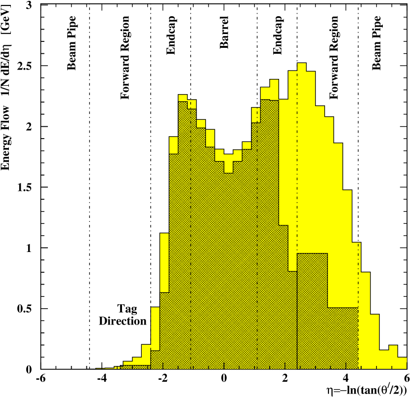
Figure 42: The general behaviour of the hadronic energy flow. The hadronic energy flow per event based on the HERWIG5.8d generator is shown as a function of the pseudorapidity $\eta$ for $\langle Q^{2}\rangle=13$ $\mathrm{GeV^{2}}$. The observed electron is always at negative rapidities, $-3.5<\eta<-2.8$, and is not shown. The dark shaded histogram represents the energy reconstructed by the OPAL detector after the simulation of the detector response to the HERWIG5.8d events. The generated energy distribution for these events is represented by the lightly shaded histogram. The vertical lines show the acceptance regions of the OPAL detector components.

The flow of hadronic energy as a function of the pseudorapidity, for an average event, $1/N~{}{\rm d}E/{\rm d}\eta$, is shown in Figure 42, taken from Ref. [87]. The generated hadronic energy flow as predicted by the HERWIG5.8d Monte Carlo is compared to the visible flow of the hadronic energy as observed after simulating the response of the OPAL detector. The hadronic energy flow sums over all charged and neutral particles. The pseudorapidity is defined as $\eta=-\ln(\tan(\theta^{\prime}/2))$, where $\theta^{\prime}$ is the polar angle of the particle measured from the direction of the beam that has produced the quasi-real photon, so the observed electron is at $-3.5<\eta<-2.8$, but is not shown. This figure demonstrates that a significant fraction of the energy flow in events from the HERWIG5.8d generator goes into the forward region of the detector. About two thirds of the energy is deposited in the central region of the detector, and 30$\%$ goes into the forward region. As little as 5$\%$ of the total hadronic energy is lost in the beampipe.

Figure 43: The correlation between the measured and generated hadronic invariant mass. The correlation between the generated hadronic invariant mass $W$ and the visible mass $W_{\mathrm{vis}}$ with and without the hadronic energy sampled in the forward region (FR) of the OPAL detector. In (a) the correlation is shown for HERWIG5.8d and (b) for F2GEN; in each case for two cuts on the minimum polar angle of the acceptance region. The symbols represent the average $W_{\mathrm{vis}}$ in each bin, and the vertical error bar its standard deviation. The dashed line corresponds to a perfect correlation $W_{\mathrm{vis}}=W$.

The reconstructed energy flow is rather similar to the generated energy flow in the central region, but significantly different in the forward region. The small inefficiency in the central detector region is mostly due to the fact that some hadrons in this region carry low energy, and therefore fail quality cuts applied to the events in the experimental analyses. The forward regions of the LEP detectors are only equipped with electromagnetic calorimeters and the hadronic energy in the forward region can only be sampled by using these electromagnetic calorimeters. Consequently, for example in the case of the OPAL detector, only about 42$\%$ of the total hadronic energy in the forward region can be recovered, with an energy resolution of $\Delta E/E=30\%$ of the seen energy, as explained in Ref. [87]. Given this, the detectors are precise enough to disentangle various predictions in the central part of the detector. However, they are not able to distinguish well between models which produce different energy flow distributions in the forward region.

The different Monte Carlo models produce rather different hadronic energy flows also within the clear acceptance of the detectors, which leads to the fact that for a given value of $W$, the visible invariant mass $W_{\mathrm{vis}}$ is rather different when using different Monte Carlo models. The correlation between the generated and visible invariant masses is shown in Figure 43, taken from Ref. [87], for two Monte Carlo models described in Section 5.1. The level of correlation achieved between $W_{\mathrm{vis}}$ and $W$, strongly depends on the acceptance region for the hadronic final state and also on the model chosen. A Monte Carlo model like F2GEN predicts a much stronger correlation than, for example, the HERWIG5.8d Monte Carlo model. This strongly effects the acceptance of the events and therefore the $x_{\mathrm{vis}}$ distributions, especially at low values of $x_{\mathrm{vis}}$ and correspondingly low values of $x$.

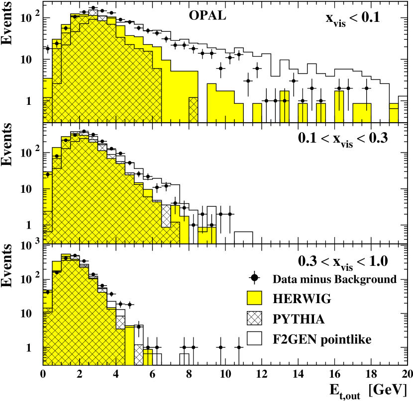
Figure 44: The measured $E_{\mathrm{t,out}}$ distribution for $\langle Q^{2}\rangle=13$ $\mathrm{GeV^{2}}$ in bins of $x$. The energy transverse to the plane defined by the beam axis and the momentum vector of the observed electron, $E_{\mathrm{t,out}}$, is shown at the detector level for three ranges in $x_{\mathrm{vis}}$.

The differences of the predictions can most clearly be seen in variables like the energy transverse to the plane defined by the beam axis and the momentum vector of the observed electron, $E_{\mathrm{t,out}}$, which is shown in Figure 44, taken from Ref. [87], in bins of $x_{\mathrm{vis}}$. The value of $E_{\mathrm{t,out}}$ is obtained by summing up the absolute values of the energy transverse to the tag plane for all objects. The F2GEN model predicts the hardest spectrum and lies above the data, whereas the HERWIG5.8d model lies below the data and the PYTHIA prediction does not even populate the tail of the $E_{\mathrm{t,out}}$ distribution. It is apparent from this figure that the largest differences occur at low values of $x_{\mathrm{vis}}$. Taking the differences of the models into account in a bin-by-bin correction procedure the observed hadronic energy flow can be corrected to the hadron level and compared to various model predictions. Examples of this are shown in Figure 45 for $\langle Q^{2}\rangle=13$ $\mathrm{GeV^{2}}$, and in Figure 46 for $\langle Q^{2}\rangle=135$ $\mathrm{GeV^{2}}$, both taken from Ref. [87]. The errors take into account the dependence of the correction on the Monte Carlo model chosen for correcting the data. A detailed discussion of the various models used can be found in Section 5.1. The shape of the hadronic energy flow drastically changes from a two peak structure at low values of $Q^{2}$ to a one peak structure for increasing $Q^{2}$, which also means increasing values of $x$. The differences between the models shrink considerably, and in addition the predictions lie much closer to the data. This shows firstly that the problem is located in the region of low values of $x$ and large values of $W$, and secondly that the data are certainly precise enough to further constrain the models. None of the models shown is able to describe the data at $\langle Q^{2}\rangle=13$ $\mathrm{GeV^{2}}$, but the agreement improves for $\langle Q^{2}\rangle=135$ $\mathrm{GeV^{2}}$.

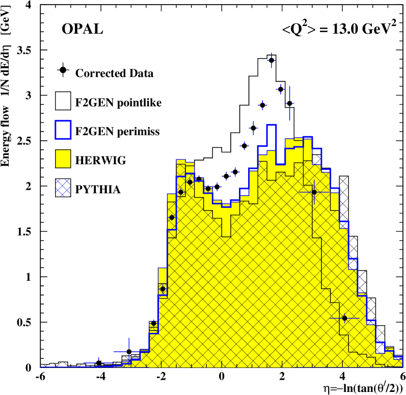
Figure 45: The corrected hadronic energy flow for $\langle Q^{2}\rangle=13$ $\mathrm{GeV^{2}}$. The measured energy flow per event is corrected for the detector inefficiencies, as a function of pseudorapidity $\eta$, and compared to the generated energy flow of the HERWIG5.8d and PYTHIA Monte Carlo models and the energy flow of samples of point-like and perimiss events from the F2GEN model. The vertical error bars on the data points are the sum of the statistical and systematic errors, and the horizontal bars indicate the bin widths.

After these findings were reported, several methods were investigated to reduce the dependence of the measured $F_{2}^{\gamma}$ on the Monte Carlo models. A first attempt to improve on the HERWIG5.9 model was made in Refs. [158, 148] by altering the distribution of the transverse momentum, $k_{\mathrm{t}}$, of the quarks inside the photon from the program default. The default Gaussian behaviour was replaced by a power-law function of the form $\mathrm{d}k^{2}_{\mathrm{t}}/(k^{2}_{\mathrm{t}}+k_{0}^{2})$ with $k_{0}=0.66$ GeV, motivated by the observation made in photoproduction studies at HERA that a better description of the data is achieved if the intrinsic transverse momentum distribution is changed to the power-law behaviour, as explained in Ref. [159]. The upper limit of $k^{2}_{\mathrm{t}}$ in HERWIG5.9+$k_{\mathrm{t}}$ was fixed at $k^{2}_{\mathrm{t,max}}=25$ GeV², which is almost the upper limit of $Q^{2}$ for the OPAL analysis from Ref. [87]. This led to some improvements in the description of the OPAL data by the HERWIG5.9+$k_{\mathrm{t}}$ Monte Carlo, as reported, for example, in Ref. [158].

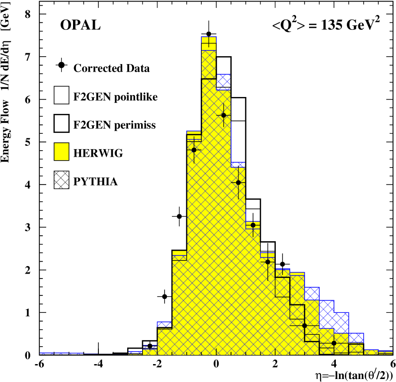
Figure 46: The corrected hadronic energy flow for $\langle Q^{2}\rangle=135$ $\mathrm{GeV^{2}}$. Same as Figure 45 but for $\langle Q^{2}\rangle=135$ $\mathrm{GeV^{2}}$.

A second attempt to improve on the situation is based on a purely kinematic consideration already explained in Ref. [123]. The longitudinal momentum of the photon-photon system is unknown, but the transverse momentum is well constrained by measuring the transverse momentum of the scattered electron. In addition, when the $+z$ axis is chosen in the hemisphere of the observed electron, the unseen electron which radiated the quasi-real photon escapes with $E_{2}^{\prime}-|p_{2,\rm z}^{\prime}|\approx 0$ along the beam line. Here $E_{2}^{\prime}$ and $p_{2,\rm z}^{\prime}$ denote the energy and longitudinal momentum of the unseen electron. This fact can be used to replace $E_{\mathrm{had}}+p_{\mathrm{z,had}}$, the sum of the energy and longitudinal momentum of the total hadronic system, by quantities obtained from the scattered electron.

Figure 47: Comparison of different methods for the reconstruction of the invariant mass of the hadronic final state. Shown are the generated mass $W=W_{\gamma\gamma}$, the visible mass obtained from the observed hadrons in the L3 detector, $W_{\mathrm{vis}}$ and $W_{\mathrm{rec}}$, defined in Eq. (53). All distributions are for the PHOJET Monte Carlo model in the $Q^{2}$ range $1.2-9$ $\mathrm{GeV^{2}}$.

If in addition the transverse momentum squared of the hadronic system, $p^{2}_{\mathrm{t,had}}$, is replaced by that of the scattered electron, $p_{1,\rm t}^{\prime 2}$, a part of the uncertainty of the measurement of the hadronic final state can be eliminated. The value of $W$ reconstructed in this scheme is called $W_{\mathrm{rec}}$ and has the following form

$$W_{\mathrm{rec}} = \left(E_{\mathrm{had}}+p_{\mathrm{z,had}}\right)\cdot\left(E_{\mathrm{had}}-p_{\mathrm{z,had}}\right)-p^{2}_{\mathrm{t,had}}$$ (53)

$$= \left[2E-\left(E_{1}^{\prime}+p_{1,\rm z}^{\prime}\right)\right]\left(E_{\mathrm{had}}-p_{\mathrm{z,had}}\right)-p_{1,\rm t}^{\prime 2}\,.$$

Because the quantities which are replaced depend on the properties of the hadronic final state, the improvement is expected to show some dependence on the Monte Carlo programs used. For example, for the PHOJET Monte Carlo, the improvement on the resolution in $W$ can be seen from Figure 47, taken from Ref. [89]. The generated values of $W=W_{\gamma\gamma}$ are compared to $W_{\mathrm{vis}}$ and $W_{\mathrm{rec}}$ using the PHOJET Monte Carlo model in the $Q^{2}$ range $1.2-9$ $\mathrm{GeV^{2}}$. The improvement is expected to be largest for L3, because this detector, on top of the general problems discussed above, suffers from a dead region in acceptance, as can be seen from Figure 48, taken from Ref. [89]. The distribution of $W_{\mathrm{rec}}$ is closer to the $W$ distribution than the $W_{\mathrm{vis}}$ distribution, but still the agreement with $W$ is not very good.

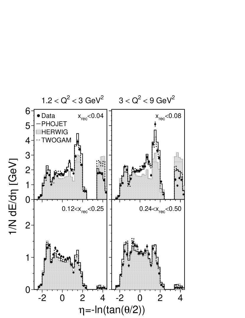
Figure 48: The measured hadronic energy flow from L3. The measured hadronic energy flow is compared to the Monte Carlo predictions in bins of $x_{\mathrm{rec}}$, obtained from $W_{\mathrm{rec}}$ and $Q^{2}$, and in bins of $Q^{2}$. The models used are HERWIG5.9+$k_{\mathrm{t}}$, PHOJET and TWOGAM.

Recently, in Ref. [89], the PHOJET Monte Carlo model has been used for the first time in a structure function analysis. Also for the first time in this analysis the TWOGAM Monte Carlo program was used outside the DELPHI collaboration. In Figure 48, taken from Ref. [89], the prediction of the hadronic energy flow for these two models are compared to the L3 data for the $Q^{2}$ range $1.2-9$ $\mathrm{GeV^{2}}$. Again, these two models, although closer to the data than the HERWIG5.8d and PYTHIA predictions in the case of the OPAL analysis, do not accurately account for the features observed in the data distributions. In the case of L3 the HERWIG5.9+$k_{\mathrm{t}}$ model, which was tuned for the $Q^{2}$ region of $6-30$ $\mathrm{GeV^{2}}$, does not provide a satisfactory description of the data taken in the region $1.2<Q^{2}<9$ $\mathrm{GeV^{2}}$, and therefore the L3 analysis of the photon structure function $F_{2}^{\gamma}$ is only based on the PHOJET and TWOGAM models.

The above information is valuable in understanding the discrepancies, however, the investigations suffer from three main shortcomings. Firstly, always slightly different cuts are applied to the experimental data, and therefore, although the data are rather indicative, it is not clear, whether a consistent picture emerges from the results of the different experiments. Secondly, in the present form, the data cannot be directly compared to the generated quantities obtained without simulating the detector response. This is because either the data are not corrected for detector effects, as in the case of L3, Figure 48, or they still depend on cuts applied to the data, which is the case for the OPAL distributions, Figures 45 and 46, which are only obtained for events fulfilling the experimental cuts applied at the detector level. However, in order for the authors to improve on their models it is mandatory that they can compare to corrected distributions provided by the experiments, without the need of simulating the detector response. Thirdly, it is hard to get a reliable estimate of the systematic error of the experimental result within one experiment, because in this case it can only be obtained from varying the Monte Carlo predictions using models which do not accurately describe the data, certainly not a very reliable method.

To overcome these shortcomings a combined effort by the ALEPH, L3 and OPAL collaborations and the LEP Working Group for Two-Photon Physics has been undertaken, and preliminary results of this work have been reported in Ref. [149]. The data of the experiments have been analysed in two regions of $Q^{2}$, $1.2-6.3$ $\mathrm{GeV^{2}}$ and $6-30$ $\mathrm{GeV^{2}}$, using identical cuts and also identical Monte Carlo events passed through the respective programs of the individual experiments to simulate the detector response. The data are corrected to the hadron level in a phase space region which is purely determined by cuts at the hadron level, and the systematic error is estimated by the spread of the corrected distributions of the three experiments. Then the data are compared to predictions from the HERWIG5.9+$k_{\mathrm{t}}$ and the PHOJET Monte Carlo models. Several distributions are studied, namely, the reconstructed invariant hadronic mass, defined within a restricted range in polar angles, the transverse energy out of the plane defined by the beam direction and the direction of the observed electron, the number of tracks, the transverse momenta of tracks with respect to the beam axis, and the hadronic energy flow as a function of the pseudorapidity. Preliminary results of this investigation have been reported in Ref. [149]. It is found that for large regions in most of the distributions studied, the results of the different experiments are closer to each other than the sizeable differences which are observed between the data and the models. Since the data distributions are corrected to the hadron level, they can be directly compared to the predictions of the Monte Carlo models. Therefore the combined LEP data serve as an important input to improve on the Monte Carlo models. The investigation already led to an improved version of the HERWIG5.9+$k_{\mathrm{t}}$ program obtained by again altering the modelling of the intrinsic transverse momentum of the quarks within the photon. While the fixed limit of $k^{2}_{\mathrm{t,max}}=25$ GeV² was adequate for the region $6<Q^{2}<30$ $\mathrm{GeV^{2}}$, for lower values of $Q^{2}$, it introduces too much transverse momentum. This has been overcome by dynamically adjusting the upper limit of $k_{\mathrm{t}}$ by the event kinematic on an event by event basis. In this scheme, called HERWIG5.9+$k_{\mathrm{t}}$ (dyn) the maximum transverse momentum is set to $k^{2}_{\mathrm{t,max}}\approx Q^{2}$. This change leads to an improved description of the data also for the region $1.2<Q^{2}<6.3$ $\mathrm{GeV^{2}}$.

Another way of reducing the model dependence of the measured $F_{2}^{\gamma}$ is to perform the unfolding in two dimensions, as described in Section 5.2. Recent preliminary results from the ALEPH and OPAL experiments, presented in Refs. [160] and [161] respectively, show that this indeed reduces the systematic uncertainty on the structure function measurements.

From the discussion above it is clear that the error on the measurement of $F_{2}^{\gamma}$ will vary strongly with the selection of Monte Carlo models chosen to obtain the size of the systematic uncertainty. However, given the improved understanding of the shortcomings and the combined effort in improving on the Monte Carlo description of the data, it is likely that the error on $F_{2}^{\gamma}$ will shrink considerably in future measurements. This closes the discussion about the description of the hadronic final state by the Monte Carlo models, and the measurements of $F_{2}^{\gamma}$ will be discussed next.

7.2 Hadronic structure function $F_{2}^{\gamma}$

Many measurements of the hadronic structure function $F_{2}^{\gamma}$ have been performed at several $\mathrm{e^{+}}\,\mathrm{e^{-}}$ colliders. Because in some cases it is not easy to correctly derive the errors of several of the measurements, a detailed survey of the available results has been performed, the outcome of which is presented in Appendix D. The measurements and what can be learned from them about the structure of the photon and on its description by perturbative QCD is discussed in the following. The interpretation of the data will only be based on published results, and on preliminary results from the LEP experiments, which are likely to be published soon. In contrast the preliminary results from Refs. [96, 105, 104, 106, 113], which were used in the fit procedures of several of the parton distribution functions of the photon, but which never got published, are regarded as obsolete, and will not be considered here. In all summary figures presented below only those preliminary results from the LEP experiments are included which are based on data which have not yet been published. For the preliminary results which are meant to replace a previous measurement in the near future the previously published result will be shown until the new result is finalised.

Figure 49: Measurements of the hadronic structure function $F_{2}^{\gamma}$ except from LEP. The points represent the data with their statistical (inner error bars) and total errors (outer error bars), if available, otherwise only the full errors are shown. The measured data are shown in comparison to the prediction of $F_{2}^{\gamma}$ obtained from the GRV higher order parton distribution function, using the $Q^{2}$ values given in brackets.

The range in $\langle Q^{2}\rangle$ covered by the various experiments is $0.24<\langle Q^{2}\rangle<400$ $\mathrm{GeV^{2}}$, which is impressive given the small cross section of the process. The published results from the ALEPH [162], AMY [84, 85], DELPHI [86], JADE [67], L3 [89, 163], OPAL [87, 90, 91], PLUTO [68, 69], TASSO [70], TPC/2$\gamma$ [72] and TOPAZ [71] experiments can be found in Tables 21$-$ 30. The additional preliminary results from the ALEPH [160], L3 [164] and DELPHI [165, 166] experiments are listed in Tables 31$-$33

In the present investigations of the photon structure function $F_{2}^{\gamma}$ two distinct features of the photon structure are investigated. Firstly, the shape of $F_{2}^{\gamma}$ is measured as a function of $x$ at fixed $Q^{2}$. Particular emphasis is put on measuring the low-$x$ behaviour of $F_{2}^{\gamma}$ in comparison to $F_{\mathrm{2}}^{\mathrm{p}}$ as obtained at HERA. Secondly, the evolution of $F_{2}^{\gamma}$ with $Q^{2}$ is investigated. As explained in Section 3.4, this evolution is predicted by QCD to be logarithmic. These two issues are discussed.

Figure 50: Comparison of measurements of $F_{2}^{\gamma}$ at low values of $Q^{2}$. The OPAL data at $\langle Q^{2}\rangle$ of 1.86 and 3.76 $\mathrm{GeV^{2}}$ are compared to previous results from the PLUTO and TPC/2$\gamma$ experiments. The points represent the OPAL data with their statistical (inner error bars) and total errors (outer error bars). For the previous data only the total errors are shown. The tic marks at the top of the figures indicate the bin boundaries of the OPAL analysis.

The collection of measurements on $F_{2}^{\gamma}$ which have been performed at $\mathrm{e^{+}}\,\mathrm{e^{-}}$ centre-of-mass energies below the mass of the $Z$ boson is shown in Figure 49. Their precision is mainly limited by the statistical error and, due to the simple assumptions made on the hadronic final state, the systematic errors are small, but in light of the discussion above, they may be underestimated. The global behaviour of the data is roughly described, for example, by the $F_{2}^{\gamma}$ obtained from the GRV higher order parton distribution function. However, some of the data show quite unexpected features. For example, the structure function as obtained from the TPC/2$\gamma$ experiment shows an unexpected shape at low values of $x$, and also the results from TOPAZ rise very fast towards low values of $x$. In addition there is a clear disagreement between the TASSO and JADE data at $\langle Q^{2}\rangle=23-24$ $\mathrm{GeV^{2}}$. Certainly at this stage much more data were needed to clarify the situation.

Figure 51: Preliminary update of $F_{2}^{\gamma}$ at low values of $Q^{2}$ from OPAL. The preliminary OPAL data at $\langle Q^{2}\rangle$ of 1.9 and 3.8 $\mathrm{GeV^{2}}$ are compared to the results from the PLUTO and L3 experiments. The points represent the data with their statistical (inner error bars) and total errors (outer error bars). For the PLUTO result only the total errors are shown. For the L3 result the errors are obtained as explained in Table 25.

The measurement of $F_{2}^{\gamma}$ has attracted much interest at LEP over the last years. The LEP Collaborations have measured the photon structure function $F_{2}^{\gamma}$ in the range $0.002<x$ $\stackrel{{\scriptstyle<}}{{\scriptstyle{\sim}}}$ 1 and $1.86<\langle Q^{2}\rangle<400$ $\mathrm{GeV^{2}}$. The first published result of the low-$x$ behaviour of $F_{2}^{\gamma}$ at low values of $Q^{2}$ performed on a logarithmic scale in $x$ is shown in Figure 50. The data have been unfolded based on the HERWIG5.8d Monte Carlo model. Only a weak indication of a possible rise at low values of $x$ for $Q^{2}<4$ $\mathrm{GeV^{2}}$ is observed. More important, the data seem to be consistently higher than what is predicted by the GRV and SaS1D parametrisations. In addition, there emerges an inconsistency at $Q^{2}\approx 4$ $\mathrm{GeV^{2}}$, between the OPAL and PLUTO data of Refs. [91] and [68] on one hand, and the TPC/2$\gamma$ data of Ref. [72] on the other hand.

Figure 52: The measurements of $F_{2}^{\gamma}$ at low values of $Q^{2}$ from L3. The points represent the L3 data with their total experimental errors, but excluding the large error stemming from the choice of Monte Carlo model. The models chosen for the unfolding of $F_{2}^{\gamma}$ from the data are PHOJET (set1) and TWOGAM (set2).

Recently a preliminary update of the OPAL measurement at low values of $Q^{2}$, shown in Figure 51, has been presented in Ref. [161]. The new OPAL analysis is based on the same data as the published results, but uses the PHOJET and the improved HERWIG5.9+$k_{\mathrm{t}}$ Monte Carlo models explained above, which much better describe the experimentally observed distributions than the HERWIG5.8d model used for the results in Figure 50. In addition the method of two-dimensional unfolding based on the GURU program has been explored. With these improvements the systematic errors could be considerably reduced and now, this new measurement is consistent with the GRV leading order prediction. By repeating the analysis with the HERWIG5.8d Monte Carlo model, but using two-dimensional unfolding, the new analysis leads to results consistent with the published results from Ref. [91], however with reduced errors. From this it can be concluded that firstly, the high values of the published results are due to the bad description of the data by the HERWIG5.8d model, and secondly that the two-dimensional unfolding reduces the error of the measurement, even when using an inaccurate model for the unfolding of $F_{2}^{\gamma}$.

Figure 53: The first measurement of $F_{2}^{\gamma}$ for $\sqrt{s_{\rm ee}}>m_{Z}$. The structure function $F_{2}^{\gamma}$ is measured for four active flavours in four bins in $Q^{2}$ with mean values of (a) $\langle Q^{2}\rangle$ = 9 $\mathrm{GeV^{2}}$, (b) $\langle Q^{2}\rangle$ = 30 $\mathrm{GeV^{2}}$, (c) $\langle Q^{2}\rangle$ = 14.5 $\mathrm{GeV^{2}}$, and (d) $\langle Q^{2}\rangle$ = 59 $\mathrm{GeV^{2}}$. In (e) the measurement for the combined data sets of (a) and (c), and in (f) the measurement for the combined data sets of (b) and (d) is shown. The points represent the OPAL data with their statistical (inner error bars) and total errors (outer error bars). The tic marks at the top of the figures indicate the bin boundaries. The data are compared to several predictions described in the text.

A similar analysis at low values of $x$ and $Q^{2}$, shown in Figure 52, was performed by the L3 experiment in Ref. [89]. Two results for $F_{2}^{\gamma}$ were presented which differ in the model chosen for the unfolding of $F_{2}^{\gamma}$ from the data. The published results are for PHOJET (set1) and TWOGAM (set2). From the measurement it is clear that although some improved description of the hadronic final state can be achieved by the PHOJET and TWOGAM models, the model uncertainty still is the dominant error source at low values of $x$. At $Q^{2}=5$ $\mathrm{GeV^{2}}$ the LAC1 and LAC2 predictions are consistent with the L3 result. However, the L3 result is consistently higher than the SaS1D and the leading order GRV parametrisations of $F_{2}^{\gamma}$ for both values of $Q^{2}$. Given the quoted errors of the L3 result the GRV and SaS parametrisations need to be revisited. In addition, as can be seen from Figure 51, the preliminary OPAL and the L3 measurements are consistent with each other.

The measurements discussed above are based on the entire data of the LEP1 running period at $\mathrm{e^{+}}\,\mathrm{e^{-}}$ centre-of-mass energies around the mass of the $Z$ boson. The first published result based on data for $\sqrt{s_{\rm ee}}>m_{Z}$ is shown in Figure 53, taken from Ref. [90]. Due to the higher energy of the beam electrons the $Q^{2}$ acceptance of the detectors is changed, see Figure 7 and Eq. (9). As a rule of thumb the values of $Q^{2}$ accepted at LEP2 energies is about a factor of four higher than those accepted at LEP1 energies, when using the same detector device to measure the scattered electron. The results in Figure 53 cover the $\langle Q^{2}\rangle$ range from 9 to 59 $\mathrm{GeV^{2}}$. The measured $F_{2}^{\gamma}$ as a function of $x$ is almost flat within this region and the absolute normalisation of $F_{2}^{\gamma}$ is well described by the predictions of the leading order GRV (solid) and the SaS1D (dot-dash) parametrisations of $F_{2}^{\gamma}$ evaluated at the corresponding values of $\langle Q^{2}\rangle$.

Figure 53 also shows an augmented asymptotic prediction for $F_{2}^{\gamma}$ (ASYM). The contribution to $F_{2}^{\gamma}$ from the three light flavours is approximated by the leading order asymptotic form from Ref. [21], using the parametrisation given in Ref. [30]. This has been augmented by adding a point-like charm contribution and a prediction for the hadron-like part of $F_{2}^{\gamma}$ for $\Lambda_{3}=0.232$ $\mathrm{GeV}$. The point-like charm contribution has been evaluated from the leading order Bethe-Heitler formula, Eq. (41) for $P^{2}=0$ and $m_{\mathrm{c}}=1.5$ $\mathrm{GeV}$. The estimate of the hadron-like part of $F_{2}^{\gamma}$ is given by the hadron-like part of the GRV leading order parametrisation of $F_{2}^{\gamma}$ for four active flavours, and evolved to the corresponding values of $\langle Q^{2}\rangle$. It is known that the asymptotic solution has deficits in the region of low-$x$, because of the divergences in the solution which do not occur in the solution of the full evolution equations, as explained in Section 3.4. However, the asymptotic solution has the appealing feature that it is calculable in QCD, even at higher order and for medium $x$ and with increasing $Q^{2}$ it should be more reliable. In addition, at high values of $x$ and $Q^{2}$ the hadron-like contribution is expected to be small. In the region of medium values of $x$ studied in Figure 53 this asymptotic prediction in general lies higher than the GRV and SaS predictions but it is still consistent with the data. The importance of the hadron-like contribution to $F_{2}^{\gamma}$ (HAD), which is shown separately at the bottom of the figure, decreases with increasing $x$ and $Q^{2}$, and it accounts for only 15$\%$ of $F_{2}^{\gamma}$ at $Q^{2}=59$ $\mathrm{GeV^{2}}$ and $x=0.5$. The asymptotic solution increases with decreasing $\Lambda$. For $Q^{2}=59$ $\mathrm{GeV^{2}}$ and $x=0.5$ the change in $F_{2}^{\gamma}$ is $+24\%$ and $-16\%$ if $\Lambda$ is changed from $\Lambda_{3}=0.232$ $\mathrm{GeV}$ to 0.1 $\mathrm{GeV}$ and 0.4 $\mathrm{GeV}$ respectively.

Figure 54: Measurements of the hadronic structure function $F_{2}^{\gamma}$ from LEP. Same as Figure 49 but showing the results from the LEP experiments.

By now, many more measurements for $\sqrt{s_{\rm ee}}>m_{Z}$ using much higher data luminosities have been performed by the LEP experiments. All LEP measurements are displayed in Figure 54. The measurements obtained at LEP1 energies are shown with open symbols, whereas those obtained at LEP2 energies are shown with closed symbols. The varying energies of the beam electrons give the opportunity to compare data at similar $Q^{2}$ but using different detector devices to measure the scattered electron. The results are consistent with each other, which gives confidence that the systematic errors are well enough controlled.

Figure 55: Summary of measurement of the hadronic structure function $F_{2}^{\gamma}$. Same as Figure 49 but showing all available results on $F_{2}^{\gamma}$.

A summary of all measurements of $F_{2}^{\gamma}$ is shown in Figure 55. The comparison to the GRV higher order prediction of $F_{2}^{\gamma}$ shows an overall agreement, but also some regions where the prediction does not so well coincide with the data. This large amount of data, which partly is rather precise, gives the possibility to study the consistency of the predictions with the data. The quality of the agreement is evaluated by a simple $\chi^{2}$ method based on

$$\chi^{2}=\sum_{i=1}^{\mathrm{dof}}\left(\frac{F_{2,i}^{\gamma}-\langle F_{2}^{\gamma}(x,\langle Q^{2}\rangle,0)\rangle}{\sigma_{i}}\right)^{2}\,,$$ (54)

where the sum runs over all experiments, all $\langle Q^{2}\rangle$ values, and all bins in $x$. The term $F_{2,i}^{\gamma}$ denotes the measured value of $F_{2}^{\gamma}$ in the $i^{th}$ bin and $\sigma_{i}$ is its total error. The theoretical expectation is approximated by the average $F_{2}^{\gamma}$ in that bin in $x$ at $Q^{2}=\langle Q^{2}\rangle$ and at $P^{2}=0$, abbreviated with $\langle F_{2}^{\gamma}(x,\langle Q^{2}\rangle,0)\rangle$. If, as in the case of the OPAL, the experiments quote asymmetric errors, this is taken into account by chosing the appropriate error depending on whether the prediction lies above or below the measured value. The procedure is not very precise, as it does not take into account the correlation of the errors between the data points and the experiments. However, because there are common sources of errors, it is most likely that by using this method the experimental error is overestimated. Given this, the predictions which are not compatible with the data are probably even worse approximations of the data when the comparison is done more precisely. A more accurate analysis would require to study in detail the correlation between the results within one experiment, but even more difficult, the correlation between the results from different experiments. This is a major task which is beyond the scope of the comparison presented here.

The predictions used in the comparison are the WHIT parametrisations, which are the most recent parametrisations based on purely phenomenological fits to the data, and the GRV, GRSc and SaS predictions, which use some theoretical prejudice to construct $F_{2}^{\gamma}$ as detailed in Section 4. The theoretical expectation is approximated by $\langle F_{2}^{\gamma}(x,\langle Q^{2}\rangle,0)\rangle$. If $F_{2}^{\gamma}(\langle x\rangle,\langle Q^{2}\rangle,0)$, the structure function at the average value of $x$, is taken instead, the results only slightly differ, which means that the comparison is not very sensitive to the shape of $F_{2}^{\gamma}$ within the bins chosen. The results of this comparison are listed in Tables 4 and 5.

Table 4: Comparison of the GRV, GRSc and SaS1 predictions with measurements of $F_{2}^{\gamma}$. The values are calculated using all data shown in Figure 55, apart from TPC/2$\gamma$ at $\langle Q^{2}\rangle=0.24$ $\mathrm{GeV^{2}}$ which has a $\langle Q^{2}\rangle$ below the lowest value for which a parametrisation of $F_{2}^{\gamma}$ exists. Listed are the number of data points (dof) as well as the values of $\chi^{2}/\mathrm{dof}$ as calculated from Eq. (54) for the individual experiments and for all data points (all). The minimum $Q^{2}$ for the GRSc parametrisation is larger than the value for TPC/2$\gamma$ at $\langle Q^{2}\rangle=0.38$ $\mathrm{GeV^{2}}$, therefore for GRSc the number of points is only 15 and 161 for TPC/2$\gamma$ and for all data, compared to the total number of 19 and 165. For experiments which have measured $F_{2}^{\gamma}$ for $\langle Q^{2}\rangle$ values below and above 4 $\mathrm{GeV^{2}}$, in addition the $\chi^{2}/\mathrm{dof}$ values for the comparison based only on data for $\langle Q^{2}\rangle>4$ $\mathrm{GeV^{2}}$ are shown in a second row.

		GRV		GRSc	SaS
		LO	HO	LO	1D	1M
Exp.	dof	$\chi^{2}/\mathrm{dof}$
AMY	8	0.75	1.03	0.71	0.99	0.86
JADE	8	1.01	1.16	1.03	1.09	1.00
PLUTO	13	0.50	0.46	0.53	0.60	0.51
$\langle Q^{2}\rangle>4$ $\mathrm{GeV^{2}}$	10	0.55	0.38	0.60	0.71	0.61
TASSO	5	0.97	0.77	1.03	1.03	0.85
TPC/2$\gamma$	19/15	4.52	4.11	7.34	2.00	3.98
$\langle Q^{2}\rangle>4$ $\mathrm{GeV^{2}}$	3	0.54	0.67	0.92	0.40	0.58
TOPAZ	8	1.89	2.15	1.67	2.40	1.89
ALEPH	20	0.96	1.41	0.90	1.74	1.01
DELPHI	24	0.69	1.47	0.99	1.12	0.74
L3	28	2.40	2.10	1.82	3.93	2.36
$\langle Q^{2}\rangle>4$ $\mathrm{GeV^{2}}$	22	1.91	2.21	1.20	3.43	1.95
OPAL	32	0.84	0.80	0.41	1.22	0.85
$\langle Q^{2}\rangle>4$ $\mathrm{GeV^{2}}$	24	0.45	0.55	0.37	0.79	0.50
all	165/161	1.55	1.64	1.58	1.81	1.50
$\langle Q^{2}\rangle>4$ $\mathrm{GeV^{2}}$	132	0.98	1.29	0.90	1.56	1.02

Table 5: Comparison of the SaS2 and WHIT predictions with measurements of $F_{2}^{\gamma}$. Same as Table 4, but including only data with $\langle Q^{2}\rangle>Q_{0}^{2}=4$ $\mathrm{GeV^{2}}$.

		SaS		WHIT
		2D	2M	1	2	3	4	5	6
Exp.	dof	$\chi^{2}/\mathrm{dof}$
AMY	8	1.01	1.09	0.74	0.67	0.71	0.76	0.63	0.58
JADE	8	1.52	1.51	1.25	1.09	1.05	1.27	1.11	1.08
PLUTO	10	0.58	0.60	0.62	0.57	0.56	0.81	0.65	0.63
TASSO	5	0.52	0.45	0.64	0.66	0.66	0.83	0.80	0.74
TPC/2$\gamma$	3	2.38	2.50	1.83	1.53	1.26	3.02	2.23	1.55
TOPAZ	8	1.29	1.34	1.10	1.05	1.19	0.63	0.89	1.07
ALEPH	20	1.09	1.18	1.76	8.39	14.43	14.04	52.58	81.73
DELPHI	24	0.95	0.88	1.72	7.90	13.76	13.69	46.39	73.32
L3	22	1.22	1.37	0.86	1.26	1.88	3.78	9.61	11.40
OPAL	24	0.45	0.48	0.40	0.45	0.53	1.14	1.99	2.18
all	132	0.97	1.01	1.10	3.27	5.37	5.78	18.66	28.29

None of the parametrisations has difficulties to describe the AMY, JADE, PLUTO and TASSO data, and they all disfavour the TPC/2$\gamma$ results, which show an unexpected shape as function of $x$. The WHIT parametrisations predict a faster rise at low-$x$ than the GRV, GRSc and the SaS parametrisations. Therefore, the agreement with the TOPAZ data is satisfactory for the WHIT parametrisations, whereas the GRV, GRSc and the SaS1 parametrisations yield values of $\chi^{2}/\mathrm{dof}$ of around 2, and the SaS2 parametrisations lie somewhere between these extremes. For the same reason the WHIT parametrisations fail to describe the ALEPH and DELPHI data which tend to be low at low values of $x$, thereby leading to large $\chi^{2}/\mathrm{dof}$ for the WHIT parametrisations, especially for the sets WHIT4-6 which use $a=1$, as explained in Section 4. The only acceptable agreement is achieved by using the set WHIT1. The OPAL results tend to be high at low values of $x$ and also they have larger errors, therefore only the extreme cases WHIT5-6 lead to unacceptable values of $\chi^{2}/\mathrm{dof}$. The L3 experiment quotes the smallest uncertainties on their results which tend to be high at low values of $Q^{2}$. Consequently, none of the parametrisations which are valid below $Q^{2}=4$ $\mathrm{GeV^{2}}$ is able to describe the L3 data and all lead to large values of $\chi^{2}/\mathrm{dof}$. For $Q^{2}>4$ $\mathrm{GeV^{2}}$ the agreement improves but the values of $\chi^{2}/\mathrm{dof}$ are still too large, except for GRSc. For the parametrisations valid for $Q^{2}>4$ $\mathrm{GeV^{2}}$ the best agreement with the L3 data is obtained for WHIT1. This comparison shows that already at the present level of accuracy the measurements of $F_{2}^{\gamma}$ are precise enough to constrain the parametrisations and to discard those which predict a fast rise at low-$x$ driven by large gluon distribution functions.

In conclusion, for the parametrisations valid for $Q^{2}>4$ $\mathrm{GeV^{2}}$ satisfactory agreement is found with the SaS2 and the WHIT1 parametrisations, except for the measurements of TPC/2$\gamma$. For the parametrisations evolved from lower scales, agreement is found for $Q^{2}>4$ $\mathrm{GeV^{2}}$ with the exception of the L3 and TOPAZ data, and at lower values of $Q^{2}$ they are not able to account for the TPC/2$\gamma$ and L3 results.

Figure 56: The measured $Q^{2}$ evolution of $F_{2}^{\gamma}$ for three active flavours. The data with their full errors are compared to leading order predictions of $F_{2}^{\gamma}$ for the region $0.3<x<0.8$. Shown are the GRV and SaS1D parametrisations of $F_{2}^{\gamma}$, the augmented asymptotic $F_{2}^{\gamma}$ (ASYM), and the purely asymptotic prediction (Witten), described in the text. The asymptotic predictions are evaluated for $\Lambda_{3}=0.232$ $\mathrm{GeV}$.

The second topic which is extensively studied using the large lever arm in $Q^{2}$, is the evolution of $F_{2}^{\gamma}$ with $Q^{2}$. The first measurements of this type were performed for $F_{2}^{\gamma}$ for three light flavours and the contribution to $F_{2}^{\gamma}$ from charm quarks was subtracted from the data based on the QPM prediction. This was motivated by the fact that at low values of $Q^{2}$ the charm contribution is small and that the main aim of the analyses was to compare to the perturbative predictions for light quarks based on the asymptotic solution. At the time of most of the measurements no parton distribution functions of the photon were available. A summary of the published measurements of the $Q^{2}$ evolution of $F_{2}^{\gamma}(Q^{2},uds)$ is given in Table 34 and shown in Figure 56, where the point for TASSO has been obtained from combining the three middle bins listed in Table 28. The data are nicely described by the predictions from the SaS1D and GRV parametrisations of $F_{2}^{\gamma}$. The purely asymptotic prediction from Ref. [21], using the parametrisation given in Ref. [30] for $\Lambda_{3}=0.232$ $\mathrm{GeV}$ (Witten), predicts a slightly lower $F_{2}^{\gamma}$ than is seen in the data, whereas the augmented asymptotic solution (ASYM) is somewhat high compared to the data, but both are still consistent with the measured $F_{2}^{\gamma}$.

Figure 57: The measured $Q^{2}$ evolution of $F_{2}^{\gamma}$ from OPAL. The measurement of $F_{2}^{\gamma}$ is shown for four active flavours as a function of $Q^{2}$, in (a) for the range $0.1<x<0.6$, and in (b) subdivided into $0.02<x<0.10$, $0.10<x<0.25$ and $0.25<x<0.60$. In addition shown in (a) are the $F_{2}^{\gamma}$ of the GRV leading order (LO) and the SaS1D parametrisations, the $F_{2}^{\gamma}$ of the augmented asymptotic prediction (ASYM) and the result of a higher order calculation (HO), where the last two predictions are only shown for $Q^{2}>4$ $\mathrm{GeV^{2}}$. In (b) the data are only compared to the higher order prediction. The points represent the OPAL data with their statistical (inner error bars) and total errors (outer error bars). In some of the cases the statistical errors are not visible because they are smaller than the size of the symbols.

At higher values of $Q^{2}$ the charm quark contribution to $F_{2}^{\gamma}$ gets larger and today also parametrisations of $F_{2}^{\gamma}$ for four active flavours are available. Consequently, more recent analyses of the evolution of $F_{2}^{\gamma}$ with $Q^{2}$ are based on measurements of $F_{2}^{\gamma}$ for four active flavours. In addition, due to the larger statistics available, the experiments start to look into the evolution using several ranges in $x$ for the same value of $\langle Q^{2}\rangle$. The first LEP measurement of this type is shown in Figure 57, taken from Ref. [87]. In Figure 57(a) the result for the range $0.1<x<0.6$ is compared to several parametrisations of $F_{2}^{\gamma}$. Shown are the leading order (LO) predictions of the GRV and the SaS1D parametrisations, both including the contribution to $F_{2}^{\gamma}$ from massive charm quarks, and a higher order (HO) calculation provided by E. Laenen, based on the GRV higher order parametrisation for three light quarks, complemented by the contribution of charm quarks to $F_{2}^{\gamma}$ based on the higher order calculation using massive charm quarks of Ref. [52]. The differences between the three predictions are small compared to the experimental errors, and all predictions nicely agree with the data. In addition, the data are compared to the augmented asymptotic prediction as detailed above. This approximation lies higher than the data at low $Q^{2}$ and approaches the data at the highest $Q^{2}$ reached.

The evolution of $F_{2}^{\gamma}$ with $Q^{2}$ is measured by fitting a linear function of the form $a+b\,\ln(Q^{2}/\mathrm{GeV^{2}})$ to the data for the region $0.1<x<0.6$. Here $a$ and $b$ are parameters which are taken to be independent of $x$ within the bin in $x$ chosen. The fit to the OPAL data in the $Q^{2}$ range of 7.5$-$135 $\mathrm{GeV^{2}}$ yields

$$F_{2}^{\gamma}(Q^{2})/\alpha=(0.16\pm 0.05^{+0.17}_{-0.16})+(0.10\pm 0.02^{+0.05}_{-0.02})\,\ln\,(Q^{2})\,,$$

where $Q^{2}$ is in $\mathrm{GeV^{2}}$, with $\chi^{2}/\mathrm{dof}=0.77$ for the central value, as quoted in Ref. [90]. The slope $\mathrm{d}(F_{2}^{\gamma}/\alpha)/\mathrm{d}\ln Q^{2}$ is significantly different from zero but not precisely measured yet.

Figure 58: The measured $Q^{2}$ evolution of $F_{2}^{\gamma}$ from L3. The measurement of $F_{2}^{\gamma}$ is shown for four active flavours as a function of $Q^{2}$, for four ranges in $x$, $0.01<x<0.1$, $0.1<x<0.2$, $0.2<x<0.3$ and $0.3<x<0.5$. The data are compared to $F_{2}^{\gamma}$ from the leading order GRV, SaS1D, and LAC1 parametrisations. In addition shown is a fit to the data explained in the text. The points represent the L3 data with their total errors.

The photon structure function $F_{2}^{\gamma}$ is expected to increase with $Q^{2}$ for all values of $x$, but the size of the scaling violation is expected to depend on $x$, as shown in Figure 29. To examine whether the data exhibit the predicted variation in $\mathrm{d}(F_{2}^{\gamma}/\alpha)/\mathrm{d}\ln Q^{2}$, the $Q^{2}$ range 1.86$-$135 $\mathrm{GeV^{2}}$ is analysed using common $x$ ranges. Figure 57(b) shows the measurement in comparison to the higher order calculation explained above. The points of inflection of $F_{2}^{\gamma}$ for $Q^{2}$ below 15 $\mathrm{GeV^{2}}$ are caused by the charm threshold. The data show a slightly steeper rise with $Q^{2}$ for increasing values of $x$, which is reproduced by the prediction of the higher order parametrisation of $F_{2}^{\gamma}$. However, to experimentally observe the variation of $\mathrm{d}(F_{2}^{\gamma}/\alpha)/\mathrm{d}\ln Q^{2}$ with $x$ the inclusion of more data and a reduction of the systematic error are needed.

Figure 59: The measured $Q^{2}$ evolution of $F_{2}^{\gamma}$ at medium $x$. The data with their full errors are compared to the predictions based on the leading order GRV and SaS1D parametrisations and to a higher order prediction (HO), as well as to an augmented asymptotic $F_{2}^{\gamma}$ (ASYM), both described in the text, all for the range $0.1<x<0.6$. In addition shown are the leading order GRV predictions for two other ranges in $x$, $0.2<x<0.9$ and $0.3<x<0.8$.

A similar analysis performed by the L3 experiment is shown in Figure 58, taken from Ref. [163]. Unfortunately the $x$ ranges are slightly different and the data cannot easily be combined. For $x>0.2$ the L3 data are described by all shown leading order parametrisations of $F_{2}^{\gamma}$, from LAC1, SaS1D and GRV. For smaller values of $x$ some differences are seen. In the range $0.1<x<0.2$ the data show a steeper behaviour than what is predicted by the three parametrisations of $F_{2}^{\gamma}$, and for $0.01<x<0.1$ they are higher than the SaS1D and GRV predictions, but show a similar slope, whereas the $F_{2}^{\gamma}$ based on the LAC1 parametrisation predicts a much too fast rise with $Q^{2}$.

The L3 data were fitted, as explained for the OPAL result above, in two regions of $x$, $0.01<x<0.1$ and $0.1<x<0.2$, using the $Q^{2}$ range of 1.2$-$30 $\mathrm{GeV^{2}}$. The results for the two regions are

$$F_{2}^{\gamma}(Q^{2})/\alpha = (0.13\pm 0.01\pm 0.02)+(0.080\pm 0.009\pm 0.009)\ln\,(Q^{2}/\mathrm{GeV^{2}}),$$

$$F_{2}^{\gamma}(Q^{2})/\alpha = (0.04\pm 0.08\pm 0.08)+(\phantom{0}0.13\pm\phantom{0}0.03\pm\phantom{0}0.03)\ln\,(Q^{2}/\mathrm{GeV^{2}}),$$

with $\chi^{2}/\mathrm{dof}$ of 0.69 and 0.13 for the central values. The results obtained by the L3 experiment are consistent with the OPAL result, which is valid for $0.1<x<0.6$.

Figure 60: Summary of the measurements of the $Q^{2}$ evolution of $F_{2}^{\gamma}$. The data with their full errors are compared to the predictions based on the leading order GRV and SaS1D parametrisations and to an augmented asymptotic $F_{2}^{\gamma}$, described in the text. The bins used have boundaries of 0.001, 0.01, 0.1, 0.2, 0.3, 0.4, 0.6, 0.8, 0.99, with central values as shown in the figure. To separate the measurements from each other an integer value, N, counting the bin number is added to the measured $F_{2}^{\gamma}$.

A collection of all available measurements of the evolution of $F_{2}^{\gamma}$ for four active flavours and at medium values of $x$ is listed in Table 35 and shown in Figure 59. For the PLUTO result the average $F_{2,\mathrm{c}}^{\gamma}$ in the range $0.3<x<0.8$ for the $\langle Q^{2}\rangle$ values of the analyses has been added to the published three flavour result. The charm contribution has been obtained from Eq. (41), for $P^{2}=0$ and $m_{\mathrm{c}}=1.5$ $\mathrm{GeV}$. The only significant contribution from charm quarks is for $\langle Q^{2}\rangle=45$ $\mathrm{GeV^{2}}$, where $F_{2}^{\gamma}$ increases from 0.55 to 0.73. As above for the three flavour result, the point for TASSO has been obtained from combining the three middle bins listed in Table 28.

Figure 61: Measurements of the $Q^{2}$ evolution of $F_{2}^{\gamma}$ compared to a linear fit. The same data as in Figure 60 are compared to the results of linear fits using the function $a+b\,\ln(Q^{2}/\Lambda^{2})$, with $\Lambda=0.2$ $\mathrm{GeV}$ (dash) together with the errors of the fit (dot). In addition, the predictions of the leading order GRV parametrisations of $F_{2}^{\gamma}$ are shown as full lines.

Unfortunately the different experiments quote their results for different ranges in $x$ which makes the comparison more difficult because the predictions for the various ranges in $x$ start to be significantly different for $Q^{2}>100$ $\mathrm{GeV^{2}}$, as can be seen from the GRV predictions for three different ranges of $x$ shown in Figure 59. The measurements are consistent with each other and a clear rise of $F_{2}^{\gamma}$ with $Q^{2}$ is observed. Again, this rise can be described reasonably well by the leading order augmented asymptotic prediction for $\Lambda_{3}=0.232$ $\mathrm{GeV}$.

In Figure 59 only the medium $x$ region is studied. The large amount of data shown in Figure 55 enables to investigate the variation of the scaling violation as a function of $x$ in more detail. For this purpose the data from Figure 55 are displayed differently in Figure 60. The data are shown as a function of $Q^{2}$, divided in bins of $x$, with bin boundaries of 0.001, 0.01, 0.1, 0.2, 0.3, 0.4, 0.6, 0.8, 0.99 and central values as shown in the figure. Each individual measurement is attributed to the bin with the closest central value in $x$ used. To separate the measurements from each other an integer value, N, counting the bin number is added to the measured $F_{2}^{\gamma}$. The theoretical predictions are taken as the average $F_{2}^{\gamma}$ in the bin. The $Q^{2}$ ranges used for the predictions are the maximum ranges possible for $1<W<250$ $\mathrm{GeV}$ and $Q_{0}^{2}<Q^{2}<1000$ $\mathrm{GeV^{2}}$, where $Q_{0}^{2}$ is the starting scale of the evolution for the respective parametrisation of $F_{2}^{\gamma}$. The general trend of the data is followed by the predictions of the augmented asymptotic solution, and the GRV and SaS1D leading order parametrisations of $F_{2}^{\gamma}$, however, differences are seen in specific ranges in $x$ which were discussed above in connection with Figure 55.

Table 6: Fit results of the $Q^{2}$ evolution of $F_{2}^{\gamma}$. Listed are the results for the parameters $a$ and $b$ of the fit using the function $a+b\,\ln(Q^{2}/\Lambda^{2})$, with $\Lambda=0.2$ $\mathrm{GeV}$. The errors are the one $\sigma$ parameter errors as defined by the MINUIT program. The number of degrees of freedom is denoted with dof, and the correlation of the two parameters with cor.

$x$	$a\pm\sigma_{a}$	$b\pm\sigma_{b}$	dof	$\chi^{2}/\mathrm{dof}$	cor
$0.001-0.01$	$-0.02\pm 0.01$	$0.052\pm 0.004$	18	1.69	-0.95
$0.01-0.1$	$-0.04\pm 0.01$	$0.062\pm 0.003$	36	1.36	-0.94
$0.1-0.2$	$-0.08\pm 0.02$	$0.078\pm 0.004$	33	0.51	-0.92
$0.2-0.3$	$-0.18\pm 0.04$	$0.102\pm 0.009$	15	1.12	-0.95
$0.3-0.4$	$-0.28\pm 0.08$	$0.12\pm 0.02$	13	0.65	-0.97
$0.4-0.6$	$-0.44\pm 0.08$	$0.15\pm 0.01$	20	0.28	-0.98
$0.6-0.8$	$-0.21\pm 0.17$	$0.12\pm 0.03$	15	0.87	-0.98
$0.8-0.98$	$-1.4\pm 1.1$	$0.30\pm 0.15$	2	0.35	-0.99

To quantify the increasing slope as function of $Q^{2}$ for increasing values of $x$, the data are fitted, in bins of $x$ by a linear function of the form $a+b\,\ln(Q^{2}/\Lambda^{2})$, with $\Lambda=0.2$ $\mathrm{GeV}$. The results of the fit are displayed in Figure 61 and listed in Table 6. Because some of the data contain asymmetric errors, the central values and errors of the fit parameters are not obtained from analytically solving the problem, but rather the MINUIT program from Ref. [167] has been used to perform the fit. The fitted values for the parameters $a$ and $b$, as well as their errors are given. The errors are calculated as the one $\sigma$ parameter errors defined by the MINUIT program, as explained in Ref. [167]. They reflect the change of a given parameter, when the $\chi^{2}$ is changed from $\chi^{2}_{\mathrm{min}}$ to $\chi^{2}_{\mathrm{min}}+1$. The parameters $a$ and $b$ are almost 100$\%$ anticorrelated. The errors of the fitted functions are indicated in Figure 61 using the full error matrix. For comparison the GRV leading order predictions are shown as well. Although the prediction, for example, from the GRV leading order parametrisation is not compatible with such a linear approximation, the data, at the present level of accuracy, can be fitted with linear functions with acceptable values of $\chi^{2}/\mathrm{dof}$. In some cases $\chi^{2}/\mathrm{dof}$ is much smaller than unity indicating that using the full error is overestimating the errors. Consequently, the data are more precise and a combined fit with a careful estimation of the correlation of the errors should be performed soon. The results of the fits listed in Table 6, show a significant increase in slope for increasing $x$ in accordance with the theoretical expectation.

Figure 62: The $Q^{2}$ evolution of $F_{2}^{\gamma}$ for three active flavours compared to the asymptotic solution and the QPM prediction. The same data as in Figure 60 are used and the charm contribution is subtracted as explained in the text. The three flavour results are compared to the prediction of the asymptotic solution with $\Lambda_{3}=0.232$ $\mathrm{GeV}$ (Witten, full) and to the QPM prediction assuming $m_{q_{k}}=0.2$ $\mathrm{GeV}$ (QPM, dash).

To compare the data more directly to the asymptotic solution of $F_{2}^{\gamma}$, without the complication due to the heavy quark contribution, the charm quark contribution is subtracted from the measurements based on the point-like QPM prediction, Eq. (41), for $P^{2}=0$ and for a charm quark mass of $m_{\mathrm{c}}=1.5$ $\mathrm{GeV}$. In Figure 62 the three flavour result is compared to the leading order asymptotic prediction from Ref. [21], using the parametrisation given in Ref. [30], for $\Lambda_{3}=0.232$ $\mathrm{GeV}$, and to the QPM prediction for the three light quarks assuming $m_{q_{k}}=0.2$ $\mathrm{GeV}$. The values of $\chi^{2}/\mathrm{dof}$ as calculated from Eq. (54) are given in in Table 7.

Table 7: Comparison of the $Q^{2}$ evolution of $F_{2}^{\gamma}$ to the asymptotic solution and to the QPM prediction. Listed are the ranges in $x$ used, the number of data points in each range, dof, and the $\chi^{2}/\mathrm{dof}$ values for the predictions of $F_{2}^{\gamma}$ from the asymptotic solution (Witten), for $\Lambda_{3}=0.232$ $\mathrm{GeV}$ and the quark parton model (QPM), for $m_{q_{k}}=0.2$ $\mathrm{GeV}$.

		Witten	QPM
$x$	dof	$\chi^{2}/\mathrm{dof}$	$\chi^{2}/\mathrm{dof}$
$0.001-0.01$	20	14.7	56.9
$0.01-0.1$	38	16.2	18.8
$0.1-0.2$	35	3.76	2.85
$0.2-0.3$	17	2.84	1.69
$0.3-0.4$	15	1.01	1.86
$0.4-0.6$	22	1.02	1.27
$0.6-0.8$	17	0.84	0.99
$0.8-0.98$	4	0.76	1.94

At low values of $x$ both predictions undershoot the data, and the agreement improves with increasing values of $x$. For $x>0.3$ the asymptotic prediction gives a slightly better description than the QPM prediction resulting in $\chi^{2}/\mathrm{dof}$ values around 1. It is a very interesting observation that the perturbative prediction is able to describe the behaviour for large $x$ for a reasonable value of the only free parameter $\Lambda_{3}$.

To make a more quantitative statement on the description of the measured $F_{2}^{\gamma}$ by the perturbative prediction, an $x$-dependent parametrisation of the next-to-leading order asymptotic prediction must be available. Then, the data should be compared to the next-to-leading order asymptotic prediction to fix the QCD scale $\Lambda$, with a proper definition of the region of validity of this approximation to avoid the singularities. In addition, then the charm subtraction could also be based on the next-to-leading order calculation from Ref. [52]. Finally the contribution of the hadron-like component of the charm production should be investigated, especially at low values of $x$.

7.3 Hadronic structure of virtual photons

The structure functions of virtual photons can be determined in the region $Q^{2}\gg P^{2}\gg\Lambda^{2}$ by measuring the cross-sections for events where both electrons are observed. In this region Eq. (18) can be used to define an effective structure function $F_{\mathrm{eff}}^{\gamma}$ as explained in Section 3.1. Due to the $P^{2}$ suppression of the cross-section these measurements suffer from low statistics.

Figure 63: The effective photon structure function $F_{\mathrm{eff}}^{\gamma}$ from PLUTO. In (a) $F_{\mathrm{eff}}^{\gamma}$ as a function of $x$ is compared to the next-to-leading order (NLO) result of the GRS parametrisation of the parton distribution functions of virtual photons with, and without, including a hadron-like component at the starting scale of the evolution, denoted with NLO (full) and NLO ($\eta=0$) respectively. In (b) the $P^{2}$ evolution is shown in comparison to the full next-to-leading order result for three values of $x$, 0.3, 0.2 and 0.15, and in comparison to the prediction for $\eta=0$ at $x=0.15$.

The first measurement of this type has been performed by the PLUTO experiment in Ref. [6], for $\langle P^{2}\rangle=0.35$ $\mathrm{GeV^{2}}$ and $\langle Q^{2}\rangle=5$ $\mathrm{GeV^{2}}$. In Figure 63, taken from Ref. [119], the PLUTO measurement is compared to the theoretical predictions from the GRS parametrisations. In Figure 63(a) the structure function $F_{\mathrm{eff}}^{\gamma}$ as a function of $x$ is compared to three theoretical predictions in next-to-leading order. The best description of the data is obtained using the next-to-leading order result including a non-perturbative input at the starting scale of the evolution. If the hadron-like input is neglected, which corresponds to $\eta=0$, the prediction is consistently lower than the data, but still consistent with it, within the experimental errors. Also the prediction obtained by calculating $F_{\mathrm{eff}}^{\gamma}$ solely from the box diagram is still consistent with the data, although it is the lowest at high values of $x$. In Figure 63(b) the structure function $F_{\mathrm{eff}}^{\gamma}$ is shown as a function of $P^{2}$, including the result of $F_{2}^{\gamma}$ for the quasi-real photon. The measurement suggests a slow decrease with increasing $P^{2}$, but it is also consistent with a constant behaviour. The full next-to-leading order prediction is shown for three values of $x$ and, for $x=0.15$, in addition the purely perturbative solution is shown. Also for the $P^{2}$ evolution the full next-to-leading order prediction gives the best description of the data and the purely perturbative prediction is at the low end.

Figure 64: The effective photon structure function $F_{\mathrm{eff}}^{\gamma}$ from L3. In (a) the preliminary measurement of the structure function $F_{2}^{\gamma}$ for quasi-real photons is compared to the quark parton model prediction (QPM), to $F_{2}^{\gamma}$ as predicted by the GRV and AFG parametrisation of the parton distribution functions of real photons, and to a higher order calculation based on Ref. [52], denoted with LRSN. In (b) the effective structure function $F_{\mathrm{eff}}^{\gamma}$ is compared to the QPM prediction, to $F_{2}^{\gamma}$ predicted from the GRS parametrisation of the parton distribution functions of virtual photons (GRS F2), and to the full GRS prediction obtained from the GRS $F_{2}^{\gamma}$ together with the contribution of $F_{\mathrm{L}}^{\gamma}$ as given by the quark parton model.

Recently preliminary results of a similar measurement, using the full data taken at LEP1 energies, has been presented by the L3 experiment in Ref. [164]. The average virtualities for the L3 result are $\langle Q^{2}\rangle=120$ $\mathrm{GeV^{2}}$ and $\langle P^{2}\rangle=3.7$ $\mathrm{GeV^{2}}$. In Figure 64, taken from Ref. [164], the measurement of $F_{2}^{\gamma}$ for quasi-real photons and the effective structure function, both as functions of $x$, are compared to several theoretical predictions. As in the case of PLUTO the QPM result is too low compared to the data. Taking only $F_{2}^{\gamma}$ as calculated from the GRS parametrisation of the parton distribution functions of the photon, labelled as GRS F2, gets closer to the data, and the best description is found if the contribution of $F_{\mathrm{L}}^{\gamma}$, based on the prediction from the QPM, is added to this, denoted with GRS. The data show a faster rise with $x$ than any of the predictions, however with large errors for increasing $x$, which are mainly due to the low statistics available.

Figure 65: The virtuality dependence of $F_{\mathrm{eff}}^{\gamma}$. In (a) the $P^{2}$ dependence of the L3 result of $F_{\mathrm{eff}}^{\gamma}$ is compared to the quark parton model result (QPM), and in (b) the $Q^{2}$ dependence of the results from PLUTO and L3 are shown in comparison to the QPM prediction, for the average value of $\ln(\langle Q^{2}\rangle/\langle P^{2}\rangle)$, which is around three.

The $P^{2}$ evolution of the L3 result of $F_{\mathrm{eff}}^{\gamma}$ is shown in Figure 65(a). The QPM prediction is consistent in shape with the data, but the predicted $F_{\mathrm{eff}}^{\gamma}$ is too low. However, the main difference comes from $F_{2}^{\gamma}$ for $P^{2}=0$, which is not described by the quark parton model for $x<0.4$. This is expected, because in this region the hadron-like part is predicted to be largest, as can be seen from Figure 64(a). But in this region the data are even higher than the predictions of all parametrisations of $F_{2}^{\gamma}$ which do contain a hadron-like contribution. The measurement for $P^{2}>0$ cannot rule out the quark parton model prediction, although it is consistently higher and does not favour the QPM prediction. The ratio of $\langle Q^{2}\rangle$/$\langle P^{2}\rangle$ is similar for the PLUTO and the L3 measurements, leading to values for $\ln(\langle Q^{2}\rangle/\langle P^{2}\rangle)$ of 2.6 and 3.5 respectively. This enables to compare the $Q^{2}$ evolution of the two measurements, as shown in Figure 65(b), for $0.05<x<0.75$. The evolution is consistent with the expectation of the quark parton model for $\ln(Q^{2}/P^{2})=3$, and using the range $0.05<x<0.98$.

In summary a consistent picture is found for the effective structure function $F_{\mathrm{eff}}^{\gamma}$ of the virtual photon between the PLUTO and preliminary L3 data and the general features of both measurements are described by the next-to-leading order predictions. However, the data do not constrain the predictions strongly and for detailed comparisons to be made the full statistics of the LEP2 programme has to be explored.

If both photons have similar virtualities the photon structure function picture can no longer be applied and the data are interpreted in terms of the differential cross-section. Due to the large virtualities the cross-section is small and large integrated luminosities are needed to precisely measure it. The main interest is the investigation of the hadronic structure of the interaction of two virtual photons. However, the interest in performing these measurements increased considerably in the last years, because calculations in the framework of the leading order BFKL evolution equation, which sums $\ln(1/x)$ contributions, predicted a large cross-section for this kinematical range, see Refs. [168, 169, 170, 171]. The predicted cross-section is so large that already measurements with low statistics are able to decide whether the BFKL picture is in agreement with the experimental observations. Recently theoretical progress has been made in Refs. [172, 173] to also include next-to-leading order pieces in the calculations in the BFKL picture, as explained in Ref. [174]. Large negative corrections to the leading order results were found, for example, shown in Refs. [175]. Consequently, there is some doubt about the perturbative stability of the BFKL calculation. The theoretical development is underway and this should be kept in mind in all comparisons to the BFKL predictions. The most suitable region for the comparison is $W^{2}\gg Q^{2}\approx P^{2}\gg\Lambda^{2}$, which ensures similar photon virtualities and large values of 1/$x$. This is needed to ensure only little evolution in $Q^{2}$ and large contributions from $\ln(1/x)$ terms. These requirements strongly reduce the available statistics, therefore compromises have been made in these comparisons. The variable of interest is

$$Y=\ln\frac{2p\cdot q}{\sqrt{Q^{2}P^{2}}}=\ln\frac{W^{2}+P^{2}+Q^{2}}{\sqrt{Q^{2}P^{2}}}\approx\ln\frac{W^{2}}{\sqrt{Q^{2}P^{2}}}$$ (55)

where the approximation is only valid for $W^{2}\gg Q^{2},P^{2}$. However, experimentally this inequality is not very strong.

Figure 66: The hadronic cross-section for the exchange of two virtual photons from L3. The data of the L3 experiment are compared to the predictions of the PHOJET and TWOGAM Monte Carlo models and to an estimation in the framework of the quark parton model obtained from the Vermaseren Monte Carlo (JAMVG).

The first measurement in this kinematical region has been performed by the L3 experiment in Ref. [176] using data at LEP1 energies, $\sqrt{s_{\rm ee}}=91$ $\mathrm{GeV}$, and at $\sqrt{s_{\rm ee}}=183$ $\mathrm{GeV}$, and in addition preliminary results were reported recently in Ref. [177] for data taken at $\sqrt{s_{\rm ee}}=189$ $\mathrm{GeV}$. Electrons are selected for energies above 30 $\mathrm{GeV}$ at $\sqrt{s_{\rm ee}}=91$ $\mathrm{GeV}$ and for energies above 40 $\mathrm{GeV}$ at higher centre-of-mass energies. The average photon virtualities $\langle Q^{2}\rangle$,$\langle P^{2}\rangle$ are 3.5, 14 and 14.5 $\mathrm{GeV^{2}}$ respectively. The $W$ ranges used are $2-30/5-70/5-75$ $\mathrm{GeV}$ for the three centre-of-mass energies, which means the lowest values of $x$ probed are about $2-3\cdot 10^{-3}$, and the inequality $W^{2}\gg Q^{2},P^{2}$ reads $4\gg 3.5$ at LEP1 and $25\gg 14$ at LEP2 energies, when using the minimum value of $W$ and the average virtualities. The differential cross-section as a function of $Y=\ln(W^{2}/\sqrt{Q^{2}P^{2}})$ is shown in Figure 66, taken from Ref. [177]. The data are described by the TWOGAM Monte Carlo for $\sqrt{s_{\rm ee}}=91$ $\mathrm{GeV}$ and $\sqrt{s_{\rm ee}}=183$ $\mathrm{GeV}$. The PHOJET model gives an adequate description at $\sqrt{s_{\rm ee}}=183$ $\mathrm{GeV}$ and $\sqrt{s_{\rm ee}}=189$ $\mathrm{GeV}$, whereas it fails to describe the data $\sqrt{s_{\rm ee}}=91$ $\mathrm{GeV}$, probably due to the low cut in $W$ applied for this data. For low values of $W$ the PHOJET Monte Carlo is known to be not very reliable, as explained in Section 5.1. A prediction in the framework of the quark parton model obtained from the Vermaseren Monte Carlo is found to be too low at all energies. The presently predicted cross-sections by the BFKL calculation (not shown) are much higher than the measurements and are ruled out by the data.

Figure 67: The hadronic cross-section for the exchange of two virtual photons from OPAL. The data of the OPAL experiment are compared to the prediction of the PHOJET Monte Carlo model for data taken at $\sqrt{s_{\rm ee}}=189$ $\mathrm{GeV}$. In (a)$-$(c) the corrected cross-sections are shown as functions of $W$, $x$ and $Q^{2}$.

A similar analysis has been performed by the OPAL experiment. Preliminary results were presented in Ref. [178] based on data at $\sqrt{s_{\rm ee}}=189$ $\mathrm{GeV}$, for an integrated luminosity of about $170$ $\mathrm{pb}^{-1}$, with average photon virtualities of about $10$ $\mathrm{GeV^{2}}$, and for $W>5$ $\mathrm{GeV}$. The differential cross-section as functions of $W$, $x$ and $Q^{2}$, corrected to the phase space defined by $E_{1}^{\prime},E_{2}^{\prime}>65$ $\mathrm{GeV}$, $34<\theta_{1}^{\prime},\theta_{2}^{\prime}<55$ mrad, and $W>5$ $\mathrm{GeV}$, are shown in Figure 67, taken from Ref. [178]. Due to the larger electron energies required in the OPAL analysis compared to the L3 result, the reach in $W$ for OPAL is only about $W=35$ $\mathrm{GeV}$. This means the smallest value of $x$ reached is only about $8\cdot 10^{-3}$. The measured cross-section in the selected phase space is $0.32\pm 0.05({\rm stat})\,^{+0.04}_{-0.05}({\rm sys})$ $\mathrm{pb}$, compared to the predicted cross-sections of $0.17$ pb for PHOJET and $2.2/0.26$ pb based on the BFKL calculation in leading/higher order. Also for the OPAL analysis, the data at $\sqrt{s_{\rm ee}}=189$ $\mathrm{GeV}$ are perfectly described by the PHOJET model and there is no room for large additional contributions. The precision of the results on the differential cross-sections are limited by the low statistics and they can considerably be improved by using the full statistics of the LEP2 programme.

8 Future of structure function measurements

As discussed in the previous sections, the QED and the hadronic structure of the photon have been measured up to average photon virtualities of $\langle Q^{2}\rangle=130$ and $\langle Q^{2}\rangle=400$ $\mathrm{GeV^{2}}$ respectively. In the future, the analysis of the photon structure can be extended to higher photon virtualities firstly, by exploring the high luminosity of the complete LEP2 programme and secondly, by using the full potential of the planned linear collider project. The prospects of these two parts of the future of structure function measurements are discussed briefly in this section.

8.1 LEP2 programme

So far the measurements of the QED structure of the photon are based on data taken at LEP1 energies for integrated luminosities of about $100$ $\mathrm{pb}^{-1}$ per experiment and the results are mainly limited by statistics. Therefore, exploring the full integrated luminosity of $500$ $\mathrm{pb}^{-1}$ expected at LEP2 energies, a reduction of the error by about a factor of two can be expected.

For the case of the hadronic structure of the photon the situation is more difficult. Certainly the measurement can be extended to higher values of $Q^{2}$. The preliminary data from DELPHI already reach $\langle Q^{2}\rangle=400$ $\mathrm{GeV^{2}}$ and, using the full data sample at LEP2 energies, decent statistics up to $\langle Q^{2}\rangle=1000$ $\mathrm{GeV^{2}}$ can be reached. For the measurement of the hadronic structure at low values of $Q^{2}$ the situation is different. Also in future this measurement suffers from theoretical uncertainties and considerable improvement in the description of the hadronic final state by the Monte Carlo models is needed first, before the experimental measurements can get more precise.

The measurement of the hadronic structure for the exchange of two virtual photons suffers from low statistics, therefore using the expected $500$ $\mathrm{pb}^{-1}$ at LEP2 energies will help to bring down the statistical errors, but it should be kept in mind that the results for the region $Q^{2}\approx P^{2}\gg\Lambda^{2}$ are already based on about $200$ $\mathrm{pb}^{-1}$ of data.

8.2 A future linear collider

At a future linear collider the measurements of the photon structure can be extended to larger photon virtualities and larger photon-photon centre-of-mass energies. A recent discussion of the prospects of these measurements can be found in Ref. [179]. In particular the measurements of the photon structure functions can be performed at much higher values of $Q^{2}$. This is the subject of this section.

The linear collider is an extension of the existing $\mathrm{e^{+}}\,\mathrm{e^{-}}$ colliders LEP and SLC. Table 8 shows the improvements on several machine parameters which have to be achieved to arrive at a luminosity of the order of 10${}^{34}/$cm²s, which would lead to an integrated luminosity of about 100 fb^-1 per year of operation.

Table 8: Parameters for a future linear collider of the TESLA design. Some approximate values of parameters of the present LEP and SLC colliders are shown together with goals for a future linear collider of the TESLA design.

		LEP	SLC	TESLA
total length	[km]	26.7	4	33
gradient	[MV/m]	6	10	25
beam size $\sigma_{x}/\sigma_{y}$	[$\mu$m/$\mu$m]	110 / 5	1.4 / 0.5	0.845/0.019
electron energy	[GeV]	100	50	250
luminosity	[10${}^{31}/$cm2s]	7.4	0.1	5000-10000
${{\mathcal{L}}_{int}}$	[1/pb y]	200	15	20000

The linear collider, even when running under optimal conditions will produce a huge amount of background where many particles are produced especially in the forward regions of the detector. Detailed background studies for the linear collider were performed. The background sources will lead mainly to $\mathrm{e^{+}}\,\mathrm{e^{-}}$ pair creation and to hadronic background. For the $\mathrm{e^{+}}\,\mathrm{e^{-}}$ collision mode the background simulation of Ref. [180] showed that the amount of background expected per bunch crossing for the TESLA design is about $10^{5}$ $\mathrm{e^{+}}\,\mathrm{e^{-}}$ pairs with a total energy of $1.5\cdot 10^{5}$ $\mathrm{GeV}$ and about 0.13 events of the type ${\gamma\gamma}\rightarrow{\rm hadrons}$ for hadronic masses $W>5$ $\mathrm{GeV}$ with an average visible energy of 10 $\mathrm{GeV}$. To accommodate this background the main detector has to be shielded with a massive mask as shown, for example for the TESLA design, in Figure 68, taken from Ref. [180]. In addition, the photon radiation from the beam electrons will also lead to a significant energy smearing for the electrons of the beams. The prospects of structure function measurements have to be discussed in the context of this expected machine parameter dependent ’soft’ underlying background, and the energy spread of the beam electrons.

There is also a strong interest in the construction of a photon linear collider which would in several aspects be complementary to an electron linear collider. For several reactions the cross sections for incoming photons are larger than for incoming electrons of the same energy. In addition, some reactions, for example, the very important process ${\gamma\gamma}\rightarrow H$ only have sufficiently large event rates, when using the large flux of high energetic incoming photons from a photon linear collider. The linear collider, when operated in the electron-photon mode, would also be an ideal source of high energetic photons for structure function measurements, because the energy of the incoming real photons would be known rather precisely.

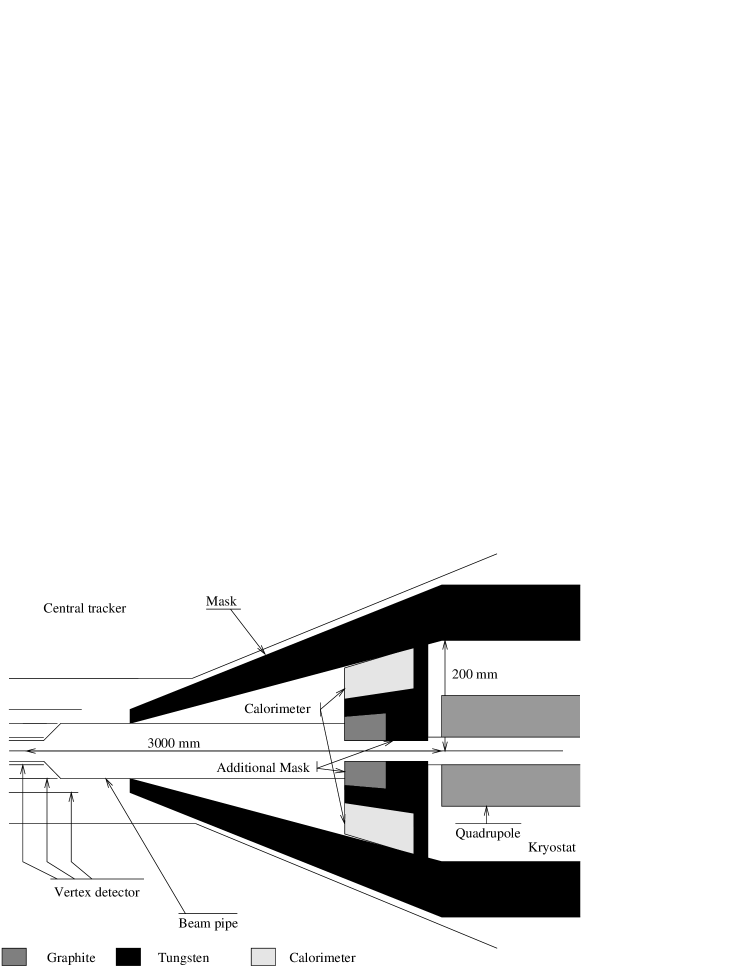
Figure 68: The forward region of a future linear collider detector. A sketch of the proposed mask to protect the detector from the background for the TESLA design.

The construction of a photon linear collider is very demanding and only general concepts are available so far. The method to produce a beam of high energetic photons from an electron beam by means of the Compton backscattering process is shown in Figure 69, taken from Ref. [181]. The photons are produced by a high intensity laser and brought into collision with the electron beams at distances of about $0.1-1$ cm from the interaction point. The photons are scattered into a small cone around the initial electron direction and receive a large fraction of the electron energy. By properly adjusting the machine parameters, like the distance along the beam line between of the production of the backscattered photons and the interaction region, by selecting the polarisations of the laser and the electron beams, and by magnetic reflection of the spent beam, the energy spectrum of the photons can be selected. As a result of this a typical distribution of ${\mathrm{e}\gamma}$ luminosity as a function of the invariant mass of the electron photon system, $\sqrt{s_{\rm e\gamma}}$, is expected to peak at the maximum reachable invariant mass of around $0.8\sqrt{s_{\rm ee}}$ with a width of 5$\%$, as described in Ref. [182].

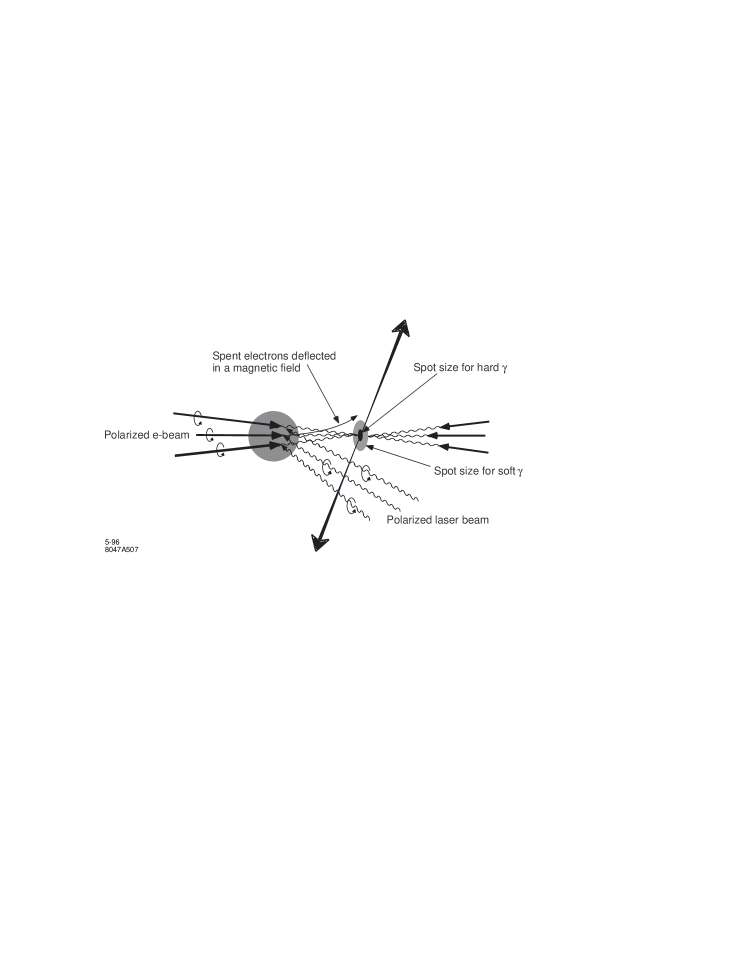
Figure 69: The production mechanism for high energetic photons. A sketch of the creation of the photon beam by Compton backscattering of laser photons off the beam electrons.

The two main questions concerning the photon structure function $F_{2}^{\gamma}$ addressed at LEP, namely the low-$x$ behaviour of $F_{2}^{\gamma}$ and the $Q^{2}$ evolution of $F_{2}^{\gamma}$ can be studied at a future linear collider but stringent requirements have to be imposed on the detector design. The region of high values of $Q^{2}$ and $x$ can already be studied with an electromagnetic calorimeter, located outside the shielding mask, and covering polar angles of the observed electrons of $\theta_{1}^{\prime}>175$ mrad, which is able to detect electrons with energies above 50$\%$ of the energy of the beam electrons, as shown in Figure 70(a,b). The errors assumed in Figure 70, taken from Ref. [183], are the quadratic sum of the statistical and the systematic components. The statistical error is calculated based on the leading order GRV structure function $F_{2}^{\gamma}$ for an integrated luminosity of 10 fb^-1. The systematic error is assumed to be equal to the statistical error but amounts to at least 5$\%$. Therefore, the precision indicated in Figure 70 has to be taken with care, as the systematic errors shown do not reflect the present level of precision of the LEP data, as detailed in Section 7. To achieve overlap in $Q^{2}$ with the LEP data the electron detection has to be possible down to $\theta_{1}^{\prime}>40$ mrad, shown in Figure 70(c,d), which means the mask has to be instrumented, and the calorimeter has to be able to detect electrons which carry 50$\%$ of the energy of the beam electrons in the huge but flat background of electron pairs discussed above, certainly a non-trivial task.

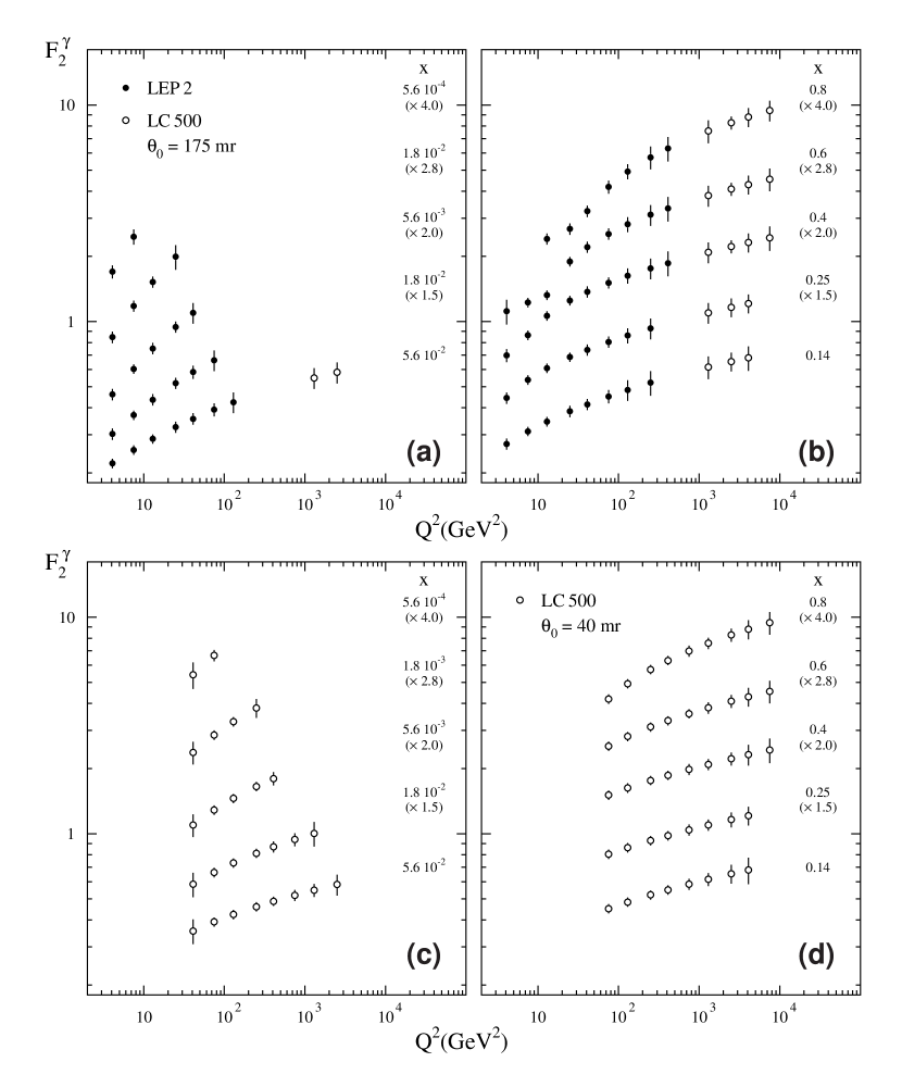
Figure 70: Prospects for structure function measurements at a future linear collider. Shown are hypothetical LEP data and linear collider data for different minimal detection angles of the deeply inelastically scattered electrons, $\theta_{1}^{\prime}$. In (a,b) $\theta_{1}^{\prime}>175$ mrad is assumed and (c,d) are based on $\theta_{1}^{\prime}>40$ mrad.

The measurement of the $Q^{2}$ evolution of the structure function $F_{2}^{\gamma}$ constitutes a fundamental test of QCD. In Figure 71 the prospects of the extension of this measurement at a future linear collider with $\sqrt{s_{\mathrm{e}{\mathrm{e}}}}=500$ $\mathrm{GeV}$ are shown for two scenarios. This figure has been taken from Ref. [179] and the measurements from PLUTO and TASSO have been added. As above, the scenarios assume that electrons can be observed for energies above 50$\%$ of the energy of the beam electrons, and for angles of $\theta_{1}^{\prime}>40$ mrad (LC1) and $\theta_{1}^{\prime}>175$ mrad (LC2). It is further assumed that the measured structure function is equal to the prediction of the leading order GRV photon structure function $F_{2}^{\gamma}$ in the respective range in $x$. The statistical errors of the hypothetical measurements are calculated from the number of events, for an integrated luminosity of 10 fb^-1, predicted by the HERWIG Monte Carlo for the leading order GRV photon structure function $F_{2}^{\gamma}$ in bins of $Q^{2}$ using the ranges in $x$ as indicated in Figure 71. The systematic error is taken to be 6.7$\%$ and to be independent of $Q^{2}$. This assumption is based on the systematic error of the published OPAL [90] result at $Q^{2}=135$ $\mathrm{GeV^{2}}$. The symmetrised value of the published systematic error is 13.4$\%$. It is assumed that this error can be improved by a factor of two. With these assumptions the error on the measurement is dominated by the systematic error up to the highest values of $Q^{2}$. It is clear from Figure 71 that overlap in $Q^{2}$ with the existing data can only be achieved if electron detection with $\theta_{1}^{\prime}>40$ mrad is possible. For $\theta_{1}^{\prime}>175$ mrad sufficient statistics is only available for $Q^{2}$ above around 1000 $\mathrm{GeV^{2}}$.

In summary with the data from the linear collider the measurement of the $Q^{2}$ evolution of the structure function $F_{2}^{\gamma}$, can be extended to about $Q^{2}=10000$ $\mathrm{GeV^{2}}$, and the low-$x$ behaviour can be investigated down to $x\approx 5\cdot 10^{-2}$ ($x\approx 5\cdot 10^{-4}$) for an electron acceptance of $\theta_{1}^{\prime}>175$ mrad ($\theta_{1}^{\prime}>40$ mrad).

Figure 71: Prospects for the measurement of the $Q^{2}$ evolution of $F_{2}^{\gamma}$ at a future linear collider. The measured $Q^{2}$ evolution of $F_{2}^{\gamma}$ is shown, together with the possible extensions at a future linear collider, denoted with LC1 and LC2. For the hypothetical data, the inner error bars indicate the statistical and the outer error bars the quadratic sum of the assumed statistical and systematic errors.

At the largest values in $Q^{2}$ also the contributions from $\mathrm{Z^{0}}$ exchange in deep inelastic electron-photon scattering could be measured and the charged-current process ${\mathrm{e}}\gamma\to\nu X$ could be used to study the weak structure of the photon. Together these measurements would allow for a separate measurement of the parton distribution functions for up and down-type quark species, as has been discussed in Ref. [184].

For a photon linear collider operating in the electron-photon mode a completely new scenario for photon structure function measurements would be opened. For the first time measurements could be performed with beams of high energetic photons of known energy with a rather small energy spread, instead of measurements using the broad bremsstrahlungs spectrum of photons radiated by electrons. With this the measurements of the photon structure function would be on a similar ground than the measurement of the proton structure function at HERA, which would probably also result in a strong reduction of the systematic error.

Another very important improvement for structure function measurements would be the detection of the electron that radiates the quasi-real photon and is scattered under almost zero angle. The possibility of such very low angle tagging is presently under study, but it is not yet clear whether it can be realised. If this could be achieved the precision of structure function measurements may significantly be improved, because $x$ could be calculated from the two detected electrons. However, it should be kept in mind that this requires a very good resolution on the measured electron energy, despite the large background discussed above, a very demanding requirement. If this could be reached the measured electron energy would be used to determine the much smaller photon energy, which would allow for a measurement of $W$ independently of the hadronic final state. Given that the dominant systematic error of the structure function measurement comes from the imperfect description of the hadronic final state by the Monte Carlo models, this would be a important step to reduce the systematic error of structure function measurements.

From the above it is clear that the investigation of the structure of the photon would greatly profit from the measurements performed at a future linear collider. However, it has to be kept in mind that at the moment it is not clear whether several of the desired features of the detector, like zero-angle tagging and excellent calorimetry inside the shielding mask, can be achieved.

9 Probing the structure of the photon apart from DIS

In addition to the results on the structure of the photon from deep inelastic electron-photon scattering the photon structure has been studied in the scattering of two quasi-real photons at $\mathrm{e^{+}}\,\mathrm{e^{-}}$ colliders, and in photoproduction and deep inelastic electron-proton scattering at HERA. These two rich fields of investigations of the photon structure cannot be covered in all details here. Only the most important topics in the context of this review will be discussed below, focusing on the general ideas and the main results. For the important details, which are not given here the reader is referred to the most recent publications and to summaries of the LEP and HERA results, which can be found in Refs. [185, 186, 187, 188].

9.1 Photon-photon scattering at $\mathrm{e^{+}}\,\mathrm{e^{-}}$ colliders

The scattering of two quasi-real photons has been studied in detail at LEP. The photon-photon scattering reaction has the largest hadronic cross-section at LEP2 energies and therefore, in most cases, the results are mainly limited by systematic uncertainties. Results have been derived on general properties of the hadronic final states in Refs. [189, 190, 191], on the total hadronic photon-photon cross-section in Refs. [176, 192, 193], on hadron production in Ref. [194], on jet cross-sections in Refs. [195, 196], on heavy quark production in Refs. [197, 198, 176, 199, 200, 122], on lepton pair production in Ref. [201] and on resonances in Refs. [202, 203, 204, 205, 206, 207, 208]. The selected topics discussed below are the total hadronic cross-section for photon-photon scattering, $\sigma_{\gamma\gamma}$, and more exclusively, hadron production, jet cross-sections and the production of heavy quarks.

9.1.1 Total hadronic cross-section for photon-photon scattering

The measurement of $\sigma_{\gamma\gamma}$ is both, interesting and challenging. It is interesting, because in the framework of Regge theory $\sigma_{\gamma\gamma}$ can be related to the total hadronic cross-sections for photon-proton and hadron-hadron scattering, $\sigma_{\mathrm{\gamma p}}$ and $\sigma_{\mathrm{hh}}$, and a slow rise with the photon-photon centre-of-mass energy squared, $W^{2}$, is predicted. It is challenging, firstly because experimentally the determination of $W$ is very difficult due to limited acceptance and resolution for the hadrons created in the reaction and secondly, because the composition of different event classes, for example, diffractive and quasi-elastic processes, is rather uncertain, which affects the overall acceptance of the events. The first problem is dealt with by determining $W$ from the visible hadronic invariant mass using unfolding programs, similarly to the measurements of the hadronic structure function. The second uncertainty is taken into account by using two models, namely PHOJET and PYTHIA, for the description of the hadronic final state and for the correction from the accepted cross-section to $\sigma_{\gamma\gamma}$, leading to the largest uncertainty of the result.

Figure 72: Published results on $\sigma_{\gamma\gamma}$ as a function of $W$.

The published measurements of $\sigma_{\gamma\gamma}$ by L3 in Ref. [191] and by OPAL in Ref. [192] are shown in Figure 72, and preliminary measurements by L3 presented in Ref. [193] are shown in Figure 73. All results show a clear rise as a function of $W$.

Figure 73: Preliminary results on $\sigma_{\gamma\gamma}$ as a function of $W$. The total hadronic cross-section for photon-photon scattering as a function of $W$ is shown for L3 data at $\sqrt{s_{\rm ee}}=189$ $\mathrm{GeV}$ and using two different Monte Carlo models for correcting the data.

The cross-section $\sigma_{\gamma\gamma}$ is interpreted within the framework of Regge theory, motivated by the fact that $\sigma_{\mathrm{\gamma p}}$ and $\sigma_{\mathrm{hh}}$ are well described by Regge parametrisations using terms to account for pomeron and reggeon exchanges. The originally proposed form of the Regge parametrisations for $\sigma_{\gamma\gamma}$ is

$$\sigma_{\gamma\gamma}(W^{2})=X_{1{\gamma\gamma}}(W^{2})^{\epsilon_{1}}+Y_{1{\gamma\gamma}}(W^{2})^{-\eta_{1}}\,,$$ (56)

where $W^{2}$ is taken in units of $\mathrm{GeV^{2}}$. The first term in the equation is due to soft pomeron exchange and the second term is due to reggeon exchange. The exponents $\epsilon_{1}$ and $\eta_{1}$ are assumed to be universal. The presently used values of $\epsilon_{1}=0.095\pm 0.002$ and $\eta_{1}=0.034\pm 0.02$ are taken from Ref. [3]. The parameters were obtained by a fit to the total hadronic cross-sections of pp, ${\rm p}\bar{{\rm p}}$, $\pi^{\pm}$p, K^±p, $\gamma$p and ${\gamma\gamma}$ scattering reactions. The coefficients $X_{1{\gamma\gamma}}$ and $Y_{1{\gamma\gamma}}$ have to be extracted from the ${\gamma\gamma}$ data. The values obtained in Ref. [3] by a fit to previous ${\gamma\gamma}$ data, including those of L3 from Ref. [191], are $X_{1{\gamma\gamma}}=(156\pm 18)$ nb and $Y_{1{\gamma\gamma}}=(320\pm 130)$ nb. Recently an additional hard pomeron component has been suggested in Ref. [209] leading to

$$\sigma_{\gamma\gamma}(W^{2})=X_{1{\gamma\gamma}}(W^{2})^{\epsilon_{1}}+X_{2{\gamma\gamma}}(W^{2})^{\epsilon_{2}}+Y_{1{\gamma\gamma}}(W^{2})^{-\eta_{1}}\,,$$ (57)

with a proposed value of $\epsilon_{2}=0.418$ and an expected uncertainty of $\epsilon_{2}$ of about $\pm 0.05$.

Figure 74: Fits to $\sigma_{\gamma\gamma}$ using various data and fit assumptions. In (a) and (b) the present theoretical predictions are shown using the central values and errors quoted in Ref. [3]. In (c) results for fits to various data as explained in the text are shown. In addition, the measurement from Ref. [192] is shown to illustrate the size of the experimental uncertainties.

Different fits to the data have been performed by the experiments. The interpretation of the results is very difficult, because, firstly, the parameters are highly correlated, secondly, the main region of sensitivity to the reggeon term is not covered by the OPAL measurement and thirdly, different assumptions have been made when performing the fits. The correlation of the parameters of Eq. (57) can be clearly seen in Figure 74(a,b), where the theoretical predictions are shown, exploring the uncertainties for the soft pomeron term in (a) and for the reggeon as well as for the hard pomeron term in (b), using the central values and errors quoted in Ref. [3]. It is clear from Figure 74(a,b) that by changing different parameters in (a) and (b) a very similar effect on the rise of the total cross-section can be achieved. Figure 74(c) shows the spread of the best fit curves for various data and various fit assumptions, explained below. In Figure 74(a-c) in addition the results from Ref. [192] are shown to illustrate the size of the experimental uncertainties.

The different fits performed by the experiments yield the following results:

• OPAL: The OPAL data taken at $\sqrt{s_{\rm ee}}=161-183$ $\mathrm{GeV}$, within the present range of $W$, can be accounted for without the presence of the hard pomeron term. When fixing all exponents and $Y_{1{\gamma\gamma}}$ to the values listed above the fit yields $X_{2{\gamma\gamma}}=(0.5\pm 0.2^{+1.5}_{-1.0})$ nb, which is not significantly different from zero, and $X_{1{\gamma\gamma}}=(182\pm 3\pm 22)$ nb, which is consistent with the values from Ref. [3]. Using $X_{2{\gamma\gamma}}=0$ and leaving only $\epsilon_{1}$ and $X_{1{\gamma\gamma}}$ as free parameters results in $\epsilon_{1}=0.101\pm 0.004^{+0.025}_{-0.019}$ and $X_{1\gamma\gamma}=(180\pm 5^{+30}_{-32})$ nb, Figure 74(c, full), again consistent with Ref. [3].

• L3: In all fits performed by L3 the hard pomeron term is set to zero. The L3 data from Ref. [191] can be fitted using the old values for the exponents of $\epsilon_{1}=0.0790\pm 0.0011$ and $\eta_{1}=0.4678\pm 0.0059$ from Ref. [210] leading to $X_{1{\gamma\gamma}}=(173\pm 7)$ nb and $Y_{1{\gamma\gamma}}=(519\pm 125)$ nb, Figure 74(c, dash). The L3 data at $\sqrt{s_{\rm ee}}=189$ $\mathrm{GeV}$ indicate a faster rise with energy. Using $\epsilon_{1}=0.95$ and $\eta_{1}=0.34$, and the PHOJET Monte Carlo for correcting the data, leads to $X_{1{\gamma\gamma}}=(172\pm 3)$ nb and $Y_{1{\gamma\gamma}}=(325\pm 65)$ nb, but the confidence level of the fit is only 0.000034. Fixing only the reggeon exponent to $\eta_{1}=0.34$ leads to $\epsilon_{1}=0.222\pm 0.019/0.206\pm 0.013$, $X_{1{\gamma\gamma}}=(50\pm 9)\,/\,(78\pm 10)$ nb and $Y_{1{\gamma\gamma}}=(1153\pm 114)\,/\,(753\pm 116)$ nb, when using PHOJET/PYTHIA, Figure 74(c, dot/dot-dash).

In summary, the situation is unclear at the moment with OPAL being consistent with the universal Regge prediction, whereas L3 indicating a faster rise with $W$ in connection with a very large reggeon component for the data at $\sqrt{s_{\rm ee}}=189$ $\mathrm{GeV}$. In addition, the L3 data taken at different centre-of-mass energies show a different behaviour of the measured cross-section, with the data taken at $\sqrt{s_{\rm ee}}=133-161$ $\mathrm{GeV}$ being lower, especially for $W<30$ $\mathrm{GeV}$.

9.1.2 Production of charged hadrons

The production of charged hadrons is sensitive to the structure of the photon-photon interactions without theoretical and experimental problems related to the definition and reconstruction of jets. The two main results from the study of hadron production at LEP are shown in Figures 75 and 76.

Figure 75: Transverse momentum distribution ${\mathrm{d}}\sigma/{\mathrm{d}}p_{\rm T}$ for hadron production in photon-photon scattering compared to other experiments. The photon-photon scattering data taken at $\sqrt{s_{\rm ee}}=161-172$ $\mathrm{GeV}$ are compared to other experiments for $10<W<30$ $\mathrm{GeV}$.

Figure 76: Transverse momentum distribution ${\mathrm{d}}\sigma/{\mathrm{d}}p_{\rm T}$ for hadron production in photon-photon scattering compared to next-to-leading order calculations. The photon-photon scattering data taken at $\sqrt{s_{\rm ee}}=161-172$ $\mathrm{GeV}$ are compared to next-to-leading order calculations for $10<W<125$ $\mathrm{GeV}$.

In Figure 75 the differential single particle inclusive cross-section ${\mathrm{d}}\sigma/{\mathrm{d}}p_{\rm T}$ for charged hadrons for ${\gamma\gamma}$ scattering from Ref. [194], with $10<W<30$ $\mathrm{GeV}$, is shown, together with results from $\gamma{\rm p}$, $\pi{\rm p}$ and ${\rm K}{\rm p}$ scattering from WA69 with a hadronic invariant mass of $16$ $\mathrm{GeV}$ from Ref. [211]. The WA69 data are normalised to the ${\gamma\gamma}$ data at $p_{\rm T}\approx 0.2$ $\mathrm{GeV}$. In addition, ZEUS data on charged particle production in $\gamma{\rm p}$ scattering with a diffractively dissociated photon from Ref. [212] are shown. These data have an average invariant mass of the diffractive system of $10$ $\mathrm{GeV}$, and again they are normalised to the OPAL data. In Figure 76 the differential single particle inclusive cross-section for $10<W<125$ $\mathrm{GeV}$ is compared to next-to-leading order QCD predictions.

The main findings are:

• The spectrum of transverse momentum of charged hadrons in photon-photon scattering is much harder than in the case of photon-proton, hadron-proton and ‘photon-Pomeron’ interactions. This can be attributed to the direct component of the photon-photon interactions.

• The production of charged hadrons is found to be described by the next-to-leading order QCD predictions from Ref. [213] over a wide range of $W$. These next-to-leading order calculations are based on the QCD partonic cross-sections, the next-to-leading order GRV parametrisation of the parton distribution functions for the photon and on fragmentation functions fitted to e⁺e^- data. The renormalisation and factorisation scales are set equal to $p_{\rm T}$.

9.1.3 Jet production

Jet production is the classical way to study the partonic structure of particle interactions. At LEP the di-jet cross-section in ${\gamma\gamma}$ scattering was studied in Ref. [196] at $\sqrt{s_{\rm ee}}=161-172$ $\mathrm{GeV}$ using the cone jet finding algorithm with $R=1$. Three event classes are defined, direct, single-resolved and double-resolved interactions. As explained in Section 1.1, direct means that the photon as a whole takes part in the hard interaction, as shown in Figure 2(a), whereas resolved means that a parton of a hadronic fluctuation of the photon participates in the hard scattering reaction, as shown in Figure 2(b,c). Experimentally, direct and double-resolved interactions can be clearly separated using the quantity

$$x_{\gamma}^{\pm}=\frac{\sum_{\rm jets=1,2}(E\pm p_{z})}{\sum_{\rm hadrons}(E\pm p_{z})},$$ (58)

whereas a selection of single-resolved events cannot be achieved with high purity. Here $E$ and $p_{z}$ are the energy and longitudinal momentum of a hadron, and the sum either runs over all hadrons in the two hard jets or over all observed hadrons. Ideally, in leading order, direct interactions have $x_{\gamma}^{\pm}=1$. However, due to resolution and higher order corrections the measured values of $x_{\gamma}^{\pm}$ are smaller. Experimentally, samples containing large fractions of direct events can be selected by requiring $x_{\gamma}^{\pm}>0.8$, and samples containing large fractions of double-resolved events by using $x_{\gamma}^{\pm}<0.8$.

Figure 77: Angular dependence of di-jet production in photon-photon scattering. The data at $\sqrt{s_{\rm ee}}=161-172$ $\mathrm{GeV}$ are compared to leading order matrix elements in (a) and to next-to-leading order (NLO) predictions in (b).

The measurement of the distribution of $\cos\theta^{\star}$ the cosine of the scattering angle in the photon-photon centre-of-mass system, allows for a test of the different matrix elements contributing to the reaction. The scattering angle is calculated from the jet rapidities in the laboratory frame using

$$\cos\theta^{\star}=\tanh\frac{\eta^{\rm jet1}-\eta^{\rm jet1}}{2}.$$ (59)

In leading order the direct contribution ${\gamma\gamma}\rightarrow q\bar{q}$ leads to an angular dependence of the form $(1-\cos^{2}\theta^{\star})^{-1}$, whereas double-resolved events, which are dominated by gluon induced reactions, are expected to behave approximately as $(1-\cos^{2}\theta^{\star})^{-2}$. The steeper angular dependence of the double-resolved interactions can be clearly seen in Figure 77(a), where the shape of the di-jet cross-section, for events with di-jet masses above $12$ $\mathrm{GeV}$ and average rapidities of $|(\eta^{\rm jet1}+\eta^{\rm jet2})/2|<1$, is compared to leading order predictions. In addition, the shape of the angular distribution observed in the data is roughly described by the next-to-leading order prediction from Refs. [214], as shown in Figure 77(b). In both cases the theoretical predictions are normalised to the data in the first three bins.

Figure 78: Transverse energy distribution ${\rm d}\sigma/{\rm d}E^{\rm jet}_{\rm T}$ for jet production in photon-photon scattering compared to next-to-leading order calculations. The measured di-jet production at $\sqrt{s_{\rm ee}}=161-172$ $\mathrm{GeV}$ is compared to next-to-leading order (NLO) predictions for different event classes.

These next-to-leading order calculations well account for the observed inclusive differential di-jet cross-section, ${\rm d}\sigma/{\rm d}E^{\rm jet}_{\rm T}$, as a function of jet transverse energy, $E^{\rm jet}_{\rm T}$, for di-jet events with pseudorapidities $|\eta^{\rm jet}|<2$.

Figure 79: Transverse energy distribution ${\rm d}\sigma/{\rm d}E^{\rm jet}_{\rm T}$ for jet production in photon-photon scattering compared to predictions for different parton distribution functions. The measured di-jet production at $\sqrt{s_{\rm ee}}=161-172$ $\mathrm{GeV}$ is compared to next-to-leading order (NLO) predictions for the GRV, GRS and GS parton distribution functions of the photon.

As expected, the direct component can account for most of the cross-section at large $E^{\rm jet}_{\rm T}$, whereas the region of low $E^{\rm jet}_{\rm T}$ is dominated by the double-resolved contribution, shown in Figure 78. The calculation for three different next-to-leading order parametrisations of the parton distribution functions of the photon are in good agreement with the data shown in Figure 79, except in the first bin, where theoretical as well as experimental uncertainties are large. Unfortunately, this is the region which shows the largest sensitivity to the differences of the parton distribution functions of the photon.

9.1.4 Heavy quark production

Similarly to the case of deep inelastic electron photon scattering discussed in Section 3.4, in photon-photon scattering the production of heavy quarks is dominated by charm quark production, because the bottom quarks are much heavier and have a smaller electric charge. Due to the large scale of the process provided by the charm quark mass, the production of charm quarks can be predicted in next-to-leading order perturbative QCD. In QCD the production of charm quarks at LEP2 energies receives sizeable contributions from the direct and the single-resolved process. In contrast, the double-resolved contribution is expected to be very small, as discussed in Ref. [215]. The direct contribution allows to test a pure QCD prediction and the single-resolved contribution is sensitive to the gluon distribution function of the photon.

In photon-photon collisions the charm quarks have been tagged using standard techniques, either based on the observation of semileptonic decays of charm quarks using identified electrons and muons in Ref. [198], or by the measurement of $D^{\star}$ production in Refs. [197, 122, 199], using the decay $D^{\star}\rightarrow D^{0}\pi$, where the pion has very low energy, followed by the D⁰ decay observed in one of the decay channels, $D^{0}\rightarrow K\pi,K\pi\pi^{0},K\pi\pi\pi$. The leptons as well as the $D^{\star}$ can be clearly separated from background processes. However, due to the small branching ratios and selection inefficiencies the selected event samples are small and the measurements are limited mainly by the statistical error.

Figure 80: Differential cross-sections for charm quark production with semileptonic decays into electrons. The data with electrons fulfilling $|\cos\theta_{\rm e}|<0.9$ and $E_{\rm e}>0.6$ $\mathrm{GeV}$ and for invariant masses $W>3$ $\mathrm{GeV}$ are compared to the prediction of the PYTHIA Monte Carlo model, normalised to the number of data events observed.

Figure 81: Differential cross-sections for charm quark production with tagged $D^{\star}$ mesons. The measured differential cross-sections for $D^{\star}$ mesons with $|\eta^{D^{\star}}|<1.5$ is compared to a next-to-leading order perturbative QCD predictions using the massless scheme.

Based on these tagging methods differential cross-sections for charm quark production and $D^{\star}$ production in restricted kinematical regions have been obtained, examples of which are shown in Figure 80 and 81. Figure 80, taken from Ref. [199], shows the differential cross-section for charm quark production, with semileptonic decays into electrons fulfilling $|\cos\theta_{\rm e}|<0.9$ and $E_{\rm e}>0.6$ $\mathrm{GeV}$ and for $W>3$ $\mathrm{GeV}$. The data are compared to the leading order prediction from PYTHIA, normalised to the number of data events observed. The shape of the distribution is well reproduced by the leading order prediction. Figure 81, taken from Ref. [122], shows the differential cross-sections for $D^{\star}$ production as a function of the transverse momentum of the $D^{\star}$, for $|\eta^{D^{\star}}|<1.5$ compared to the next-to-leading order predictions from Ref. [216] calculated in the massless approach. The differential cross-sections as functions of the transverse momentum and rapidity of the $D^{\star}$ are well reproduced by the next-to-leading order perturbative QCD predictions, both for the OPAL results presented in Ref. [122] and for the L3 results from Ref. [199]. The shape of the OPAL data can be reproduced by the NLO calculations from Ref. [215], however, the theoretical predictions are somewhat lower than the data, especially at low values of transverse momentum of the $D^{\star}$.

Based on the observed cross-sections in the restricted ranges in phase space the total charm quark production cross-section is derived, very much relying on the Monte Carlo predictions for the unseen part of the cross-section. Two issues are addressed, firstly the relative contribution of the direct and single-resolved processes, and secondly the total charm quark production cross-section. The direct and single-resolved events, for example, as predicted by the PYTHIA Monte Carlo, show a different distribution as a function of the transverse momentum of the $D^{\star}$ meson, $p_{T}^{D^{\star}}$, normalised to the visible hadronic invariant mass, $W_{\mathrm{vis}}$, as can be seen in Figure 82 from Ref. [122]. This feature has been used to experimentally determine the relative contribution of direct and single-resolved events, which are found to contribute about equally to the cross-section.

The total cross-section for the production of charm quarks is shown in Figure 83 together with previous results summarised in Ref. [16]. The figure, taken from Ref. [122], has been extended by additional L3 measurements presented in Refs. [200], by the author of Ref. [122]. The LEP results are consistent with each other and the theoretical predictions are in agreement with the data, both for the NLO prediction of the full cross-section based on the GRV parametrisation and for the leading order prediction of the direct component. The results suffer from additional errors due to the assumptions made in the extrapolation from the accepted to the total cross-section, which are avoided by measuring only cross-sections in restricted ranges in phase space. It has been shown in Ref. [215] that the NLO calculations are flexible enough to account for the phase space restrictions of the experimental analyses and that the predicted cross-sections in restricted ranges in phase space are less sensitive to variations of the charm quark mass and to alterations of the renormalisation as well as the factorisation scale. Given this, more insight into several aspects of charm quark production may be gained by comparing experimental results and theoretical predictions for cross-sections in restricted ranges in phase space.

Figure 82: The separation of the $D^{\star}$ production into direct and single-resolved contributions. The measured distribution of the transverse momentum of the $D^{\star}$ meson, $p_{T}^{D^{\star}}$, normalised to the visible hadronic invariant mass, $W_{\mathrm{vis}}$, is fitted by a superposition of the predicted distributions for direct and resolved events based on the PYTHIA Monte Carlo.

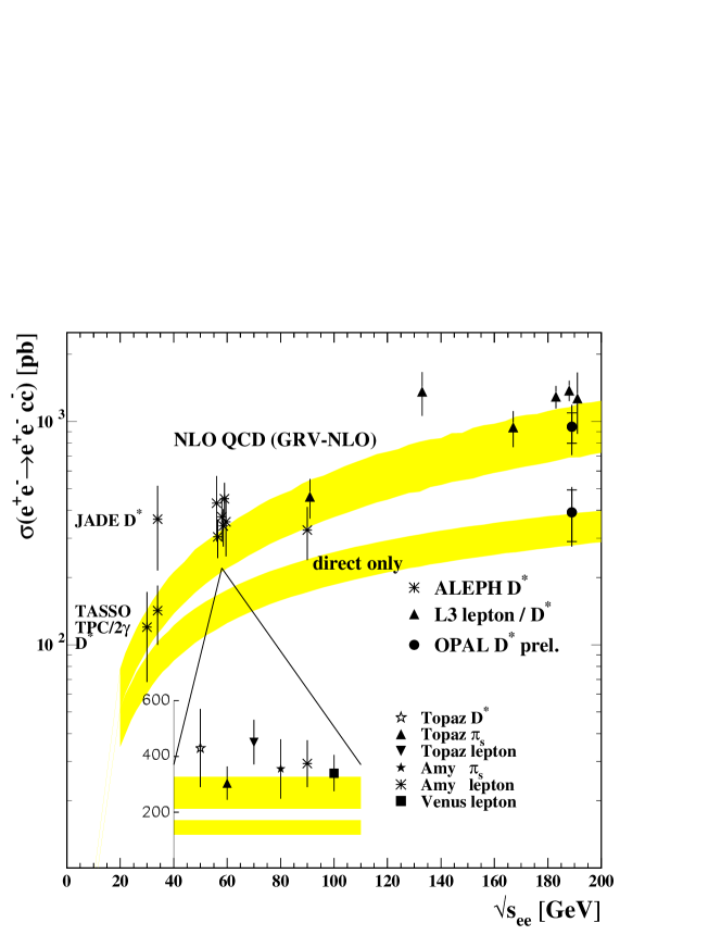
Figure 83: Total cross-section for charm quark production. The measured cross-sections from LEP using lepton tags and $D^{\star}$ tags are compared to previous measurements.

In addition to the measurements of the charm quark production cross-sections, a preliminary measurement of the cross-section for bottom quark production has been reported in Ref. [200].

9.2 Photon structure from HERA

At HERA the photon structure is investigated mainly by measurements of the total photon-proton cross-section in Refs. [217, 218, 219] and by measurements of the production of charged particles and jets in Refs. [220, 221, 222, 223, 224, 225, 226, 227, 228]. The most important results in the context of this review are the ones which try to extract information on the partonic content of quasi-real and also of virtual photons from photon-proton scattering and from deep inelastic electron-proton scattering.

At $\mathrm{e^{+}}\,\mathrm{e^{-}}$ colliders the partonic structure of the quasi-real or virtual target photon, $\gamma(P^{2},z)$, is probed by the highly virtual photon $\gamma^{\star}(Q^{2})$, in the region $Q^{2}\gg P^{2}$, as shown in Figure 3. This leads to a measurement of $F_{2}^{\gamma}(x,Q^{2})$ and, by using Eq. (38), also to a measurement of the parton distribution functions of the target photon probed at the factorisation scale $Q^{2}$. At HERA the partonic structure of the quasi-real or virtual target photon, $\gamma(P^{2},z)$, is probed by a parton from the proton, producing a pair of partons of large transverse momentum squared $p^{2}_{\mathrm{t}}$, with $p^{2}_{\mathrm{t}}\gg P^{2}$, leading, for example, to a measurement of the effective parton distribution function of the target photon, introduced in Eq. (62), probed at the factorisation scale $p^{2}_{\mathrm{t}}$. Due to the large cross-section at HERA the structure of the photon can be probed at even larger factorisation scales than at LEP. However, this is only possible if the factorisation scale is identified with the transverse momentum of the partons with respect to the photon-proton axis in the photon-proton centre-of-mass system, $Q^{2}\equiv p^{2}_{\mathrm{t}}$, which experimentally is approximated, for example, by the transverse energy squared of observed jets.

Unfortunately the variables used at HERA and LEP are denoted differently, for example at HERA the virtuality of the target photon is called $Q^{2}$ instead of $P^{2}$ and this should not be confused with the factorisation scale $Q^{2}$, which at HERA is usually taken as $p^{2}_{\mathrm{t}}$. For consistency, and to avoid confusion, in this review the factorisation scale will be denoted with $Q^{2}$, the photon virtuality with $P^{2}$, and the fractional energy of the photon from the electron, $E_{\gamma}/E$, with $z$, and the identifications will be made explicit in the figure captions.

The photon-proton scattering reaction as well as deep inelastic electron-proton scattering also depends on the structure of the proton. Therefore, the investigations of the photon structure are restricted to phase space regions where the parton distribution functions of the proton are well constrained such that the dependence on the proton structure is removed as much as possible.

There is one conceptual difference between the results obtained by ZEUS and those derived by H1. In the case of ZEUS all results are given at the hadron level, which means, the data are corrected for detector effects only. The phase space regions are selected such that hadronisation corrections, as predicted by Monte Carlo models, are expected to be small. However, the data are not corrected for these effects. The results at the hadron level are then compared to NLO calculations which are valid at the partonic level and do not contain hadronisation corrections. H1 also measures cross-sections corrected for detector effects. However, based on these cross-sections leading order partonic quantities are reconstructed, which can directly be compared to perturbative calculations at the parton level. This approach certainly reconstructs more fundamental quantities. However, they have additional uncertainties compared to the hadron level cross-sections stemming from the differences in the hadronisation procedures as assumed in the Monte Carlo programs used for the unfolding. In some cases these additional uncertainties even contribute the dominant error, as explained, for example, in Ref. [224].

Based on measurements of jet production, and charged particle production, information on the partonic structure of quasi-real and also of virtual photons have been derived. These results will be discussed in Section 9.2.1 and 9.2.2 respectively.

9.2.1 Structure of quasi-real photons

Jet cross-sections for photoproduction reactions have been measured by H1 and ZEUS.

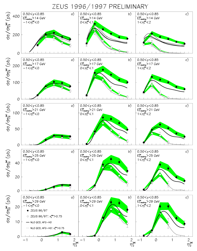
Figure 84: Di-jet cross-section in photon-proton scattering compared to next-to-leading order QCD predictions. In (a)$-$(c) the data are shown as a function of $\eta^{\rm jet2}$ in bins of $\eta^{\rm jet1}$, for $0.50<z=y<0.85$, for all selected events and for events with an observed value of $x_{\gamma}>0.75$. The rows correspond to different values for the minimum required $E^{\rm jet1}_{\rm T}$. The inner error bar indicates the statistical and the outer error bar the full error. The shaded band shows the uncertainty related to the energy scale. The curves denote the theoretical predictions based on the AFG (full), GRV (dash) and GS (dot) parametrisations of the parton distribution functions of the photon.

Figure 84, taken from Ref. [228], shows an example of a measured di-jet cross-section in electron-proton scattering from the ZEUS experiment. In this figure, additional theoretical predictions presented in Ref. [226] have been added by the author of Ref. [228]. The di-jet cross-section is corrected for detector effects and displayed for different values for the minimum required $E^{\rm jet1}_{\rm T}$. The jets are found using the $k_{\mathrm{t}}$-clustering algorithm in the inclusive mode from Ref. [229, 230], and the minimum required transverse energies of the jets are $E^{\rm jet1}_{\rm T}>14$ $\mathrm{GeV}$ and $E^{\rm jet2}_{\rm T}>11$ $\mathrm{GeV}$ for jets with $-1<\eta^{\rm jet}<2$. This ensures good stability of the next-to-leading order QCD predictions due to the asymmetric cuts on $E^{\rm jet}_{\rm T}$. The di-jet cross-section is corrected for detector effects using a bin-by-bin correction procedure. In addition, the photon virtuality is restricted to be smaller than 1 $\mathrm{GeV^{2}}$ and the scaled photon energy is required to be in the range $0.5<z<0.85$. The restriction in the photon energy enhances the sensitivity to the parton distribution functions of the photon.

The influence of the hadronisation on the di-jet cross-section has been studied based on the Monte Carlo programs HERWIG and PYTHIA. It was found that the di-jet cross-section at the parton level is 10$\%$ to 50$\%$ higher than the di-jet cross-section at the hadron level and the largest corrections are predicted for the configuration where both jets have $\eta^{\rm jet}<0$, which means the jets go in the same hemisphere as the incoming electron. In addition, based on the investigation of the transverse energy flow around the jets, it has been concluded that no inclusion of soft interactions in addition to the primary hard parton-parton scattering reaction is needed to describe the observed jet profiles at this large values of $E^{\rm jet}_{\rm T}$. This means, the jet energy profiles can be described without inclusion of the so-called soft-underlying event, a method to describe additional soft interactions between the photon and proton remnants. However, it should be noted that the predicted cross-sections of the HERWIG and PYTHIA Monte Carlo programs had to be scaled by large factors to account for the measured $x_{\gamma}$ distribution. The numbers used are 1.28/1.27 and 1.83/1.72 for the direct/resolved reactions, when using the PYTHIA and HERWIG Monte Carlo programs respectively.

The measured jet cross-section is higher than the predictions from several groups of authors, especially for the region $\eta^{\rm jet}>0$. It has been shown in Ref. [226] that the various predictions are in good agreement with each other. The cross-section shows some sensitivity to the choice of the parton distribution functions of the photon, given by the spread of the predictions seen in the first row of Figure 84.

The different regions in $\eta^{\rm jet}$ correspond to different regions in $x_{\gamma}$

$$x_{\gamma}=\frac{E^{\rm jet1}_{\rm T}\,e^{-\eta^{\rm jet1}}+E^{\rm jet2}_{\rm T}\,e^{-\eta^{\rm jet2}}}{2zE}.$$ (60)

The region of large $x_{\gamma}$ is easiest identified by the region in $\eta^{\rm jet2}$ where the curves for $x_{\gamma}>0.75$ approach those for the full range in $x_{\gamma}$. It is in this part where the parton distribution functions have the largest spread because they are only mildly constraint by the measurements of $F_{2}^{\gamma}$ shown in Figure 55. In this region the cross-section can be described by the perturbative calculations. However, for smaller values of $x_{\gamma}$, shown in Figure 84(b,c) for increasing values of $\eta^{\rm jet2}$, none of the used sets of the parton distribution functions of the photon is able to describe the data, which is taken as an indication that they may underestimate the parton content of the photon. This region corresponds to about 0.1 to 0.6 in $x_{\gamma}$, and here the constraints from the measurements of $F_{2}^{\gamma}$ are rather tight, as indicated by the small spread of the curves. It remains an interesting, but still open question, whether the parton distribution functions of the photon can be changed to describe the jet data and still being consistent with the measured $F_{2}^{\gamma}$. However, it has to be taken into account that the data are only corrected for detector effects, and thus a hadron level quantity is compared to theoretical predictions at the parton level.

Similarly, in the case of H1, the measured di-jet cross-section as a function of the average transverse energy squared of the jets in bins of $x_{\gamma}$, is the starting point to investigate the partonic structure of the photon in Ref. [222]. Again jets are found using the $k_{\mathrm{t}}$-clustering algorithm in the inclusive mode from Ref. [229, 230]. The average of the transverse energies of the two jets with the highest transverse energies is required to be above 10 $\mathrm{GeV}$ and the difference of the transverse energies should be less than 50$\%$ of their average. The average jet rapidity is constrained in the region 0-2 and the absolute difference to be smaller than unity. This ensures $E^{\rm jet}_{\rm T}>7.5$ $\mathrm{GeV}$ and, as above for the ZEUS measurement, good stability of the next-to-leading order QCD predictions. The cross-section is integrated for $P^{2}<4$ $\mathrm{GeV^{2}}$ and $0.2<z<0.83$. The measured differential electron-proton di-jet cross-section is shown in Figure 85, taken from Ref. [222]. The di-jet cross-section is corrected for detector effects only, and compared to the predictions of the leading order PYTHIA Monte Carlo and to the next-to-leading order parton level predictions using the GRV and the GS parton distribution functions of the photon. The predictions well account for the observed jet cross-section with the exceptions of low and large values of $x_{\gamma}$. For $x_{\gamma}<0.2$ the next-to-leading order prediction based on the GRV parametrisations is lower than the data, whereas the GS parametrisations are able to describe the observed cross-section. As in the case of ZEUS, for large values of $x_{\gamma}$ the GRV and GS predictions tend to lie below the data, with GS predicting a smaller cross-section due to the strongly suppressed quark distribution functions at large values of $x$ discussed in Section 4. However, for H1 the disagreement seems to be less pronounced and also to be more concentrated at larger values of $x_{\gamma}$, $0.6<x_{\gamma}<0.75$. In the highest bin in $x_{\gamma}$ and at low values of $E^{\rm jet}_{\rm T}$ both parametrisations predict too large cross-sections.

Figure 85: Inclusive di-jet cross-section for photon-proton scattering from H1. The data are shown as a function of the average transverse energy squared of the jets for several bins in $x_{\gamma}$. The inner error bars represent the statistical errors, the outer error bars the full errors. The data are compared to the leading order prediction from the PYTHIA generator (dash), and to analytical next-to-leading calculations using the GRV (full) and the GS (dot) parton distribution functions of the photon.

This cross-section is then used to determine an effective parton distribution function of the photon. The reaction is factorised into the radiation of the photon off the incoming electron, followed by a subsequent photon-proton scattering reaction. The flux of transverse photons is described using the Weizsäcker-Williams approximation, Eq. (27), discussed in Section 3.2. The photon-proton cross-section is approximated using the concept of the single effective subprocess matrix element, $M_{\mathrm{SES}}$, from Ref. [231]. This leading order approach relies on the fact that the angular dependence of the matrix elements of the most important contributions to the process is very similar, as can be seen from Figure 77. Therefore the contributions to the photon-proton cross-section can be approximated by the product of the effective parton distribution functions and the $M_{\mathrm{SES}}$, leading to

$$\frac{\mathrm{d}^{4}\sigma}{\mathrm{d}z\mathrm{d}x_{\gamma}\mathrm{d}x_{\mathrm{p}}\mathrm{d}\cos\theta^{\star}}\propto\frac{1}{z}\frac{\mathrm{d}N^{\rm T}_{\gamma}}{\mathrm{d}z}\,\frac{\tilde{f}_{\gamma}(x_{\gamma},Q^{2})}{x_{\gamma}}\,\frac{\tilde{f}_{\rm p}(x_{\mathrm{p}},Q^{2})}{x_{\mathrm{p}}}\,|M_{\mathrm{SES}}(\cos\theta^{\star})|^{2},$$ (61)

with effective parton distribution functions defined as

$$\tilde{f}_{\gamma}(x_{\gamma},Q^{2}) \equiv \sum_{k=1}^{\mathrm{n_{f}}}\left[q_{k}^{\gamma}(x_{\gamma},Q^{2})+\bar{q}_{k}^{\gamma}(x_{\gamma},Q^{2})\right]+\frac{9}{4}g^{\gamma}(x_{\gamma},Q^{2}),$$ (62)

$$\tilde{f}_{\rm p}(x_{\mathrm{p}},Q^{2}) \equiv \sum_{k=1}^{\mathrm{n_{f}}}\left[q_{k}^{\rm p}(x_{\mathrm{p}},Q^{2})+\bar{q}_{k}^{\rm p}(x_{\mathrm{p}},Q^{2})\right]+\frac{9}{4}g^{\rm p}(x_{\mathrm{p}},Q^{2}).$$ (63)

Similarly to deep inelastic electron-photon scattering, the factorisation and renormalisation scales are taken to be equal in the analysis by H1. The factorisation scale $Q^{2}$ is identified with $p^{2}_{\mathrm{t}}$, the transverse momentum squared of the partons with respect to the photon-proton axis in the photon-proton centre-of-mass system. It has been verified that the factorisation of the process into the photon flux and the two effective parton distribution functions is meaningful. This has been done by showing that within the experimental uncertainty, the observed $x_{\mathrm{p}}$ distribution is independent of the measured values of $z$ and $x_{\gamma}$ for a fixed product $zx_{\gamma}$, which means a fixed energy entering the hard parton-parton scattering from the photon side. In addition, in the region of the H1 analysis it is found that the relative amount of quark and gluon initiated di-jet events agree with the weight 9/4 to better than 5$\%$.

Figure 86: Leading order effective parton distribution function of the photon from H1. The data are shown as a function of the factorisation scale $Q^{2}=\hat{p}^{2}_{\mathrm{t}}$, averaged over $x_{\gamma}$ in the ranges a) $0.2<x_{\gamma}<0.4$ and b) $0.4<x_{\gamma}<0.7$. The inner error bar indicates the statistical and the outer error bar the full error. The data are compared to several theoretical predictions explained in the text.

The evolution of the extracted leading order effective parton distribution function $x_{\gamma}\tilde{f}_{\gamma}/\alpha$ as a function of the factorisation scale $Q^{2}$ is shown in Figure 86 taken from Ref. [222] for two regions of $x_{\gamma}$, $0.2<x_{\gamma}<0.4$ and $0.4<x_{\gamma}<0.7$. The data are compared to three predictions based on the GRV parametrisation of the parton distribution functions of the photon. The predictions shown are the effective parton distribution function (full), the quark component of $\tilde{f}_{\gamma}$ (dot), and the VMD contribution to $\tilde{f}_{\gamma}$ (dash), based on the VMD prediction of $F_{2}^{\gamma}$, explained in Section 3.5. The full prediction describes the measurement. As expected, the VMD contribution is not able to account for the data, and the importance of the gluon part increases for decreasing value of $x_{\gamma}$. Under the assumption that the factorisation and renormalisation scales can be identified with the transverse momentum of the partons, and within the uncertainties of the concept of the single effective subprocess matrix element and the effective parton distribution functions, the measurement shows the universality of the parton distribution functions of the photon, which are able to describe both photon-proton scattering and deep inelastic electron-photon scattering reactions. In addition this analysis extends the measurement of the photon structure to factorisation scales of the order of $\langle Q^{2}\rangle=\langle\hat{p}^{2}_{\mathrm{t}}\rangle\approx 900$ $\mathrm{GeV^{2}}$.

The sensitivity to the gluon distribution function of the photon seen in Figure 86 can be explored in the measurement of the di-jet cross-section and by using the production of charged particles to obtain the gluon distribution function of the photon. Both methods have been used by H1 in Refs. [220, 225] and Ref. [223] respectively. The two methods are complementary. The jet cross-section receives error contributions, for example, from the accuracy of the knowledge of the energy scales of the calorimeters and from the jet definition, which are absent when using charged particles. In addition, for sufficiently large transverse momenta of the particles, the dependence on the soft underlying event is also reduced, since most of the particles produced in the soft underlying event have momenta of the order of 0.3 $\mathrm{GeV}$. In contrast, the distribution of charged particles are more sensitive to details of the hadronisation, which are integrated over when using jets. The variable $x_{\gamma}$ is either obtained from the jets using Eq. (58), or similarly, from the sum over all charged particles with transverse momentum with respect to the beam axis of more than 2 $\mathrm{GeV}$ using the relation $x_{\gamma}\approx 1/E_{\gamma}\,\sum p_{\mathrm{t}}e^{-\eta}$. Since the incoming partons of the hard scattering process cannot be identified, no distinction can be made between quark and gluon initiated processes. Therefore, both methods yield only an indirect measurement of the gluon distribution function, because the quark initiated contribution has to be subtracted based on existing parton distribution functions obtained from measurements of $F_{2}^{\gamma}$ at $\mathrm{e^{+}}\,\mathrm{e^{-}}$ colliders.

Figure 87: Measurements of the gluon distribution function of the photon from H1. The leading order gluon distribution function as a function of $x_{\gamma}$, as obtained from the charged particle cross-section is shown twice (left full circles and right open squares) for an average factorisation scale $\langle Q^{2}\rangle=\langle\hat{p}^{2}_{\mathrm{t}}\rangle=38$ $\mathrm{GeV^{2}}$, together measurements obtained from di-jet cross-sections (left open circles from Ref. [220] and right closed circles from Ref. [225]) for $\langle Q^{2}\rangle=75$ $\mathrm{GeV^{2}}$. The inner error bar indicates the statistical and the outer error bar the full error. The data are compared to several theoretical predictions explained in the text.

The results from the two methods as a function of $x_{\gamma}$ are shown in Figure 87(left,right) taken from Refs. [223] and Refs. [225] respectively. Both figures are shown because the older figure contains more comparisons to theoretical predictions. The two results, obtained from single particles and jets respectively, are consistent and the gluon distribution function is found to be small at large values of $x$ and to rise towards small values of $x$. The measured leading order gluon distribution function is consistent with the existing parametrisation from GRV. As in the case of the structure function measurements discussed in Section 7.2, the measurements disfavour the strongly rising gluon distribution functions of the photon, for example, the LAC1 gluon distribution function. In addition, the recent H1 measurements are above the SaS1D prediction which is slightly disfavoured. This is similar to the measurements of $F_{2}^{\gamma}$ shown in Figures 50 and 52 which tend to be above the SaS1D prediction. However, the preliminary update of the $F_{2}^{\gamma}$ measurement at low values of $Q^{2}$ from OPAL, Figure 52, seems to be consistent with the SaS1D prediction. Certainly more precise data is needed to draw definite conclusions, but, again these measurements shows the universality of the parton distribution functions of the photon.

This concludes the discussion of measurements of the structure of quasi-real photons and the remaining part is devoted to virtual photons.

9.2.2 Structure of virtual photons

As has been discussed in Section 7.3 the structure of the virtual photon can be studied via the measurement of photon structure functions in the kinematical regime $Q^{2}\gg P^{2}\gg\Lambda^{2}$. The evolution of $F_{2}^{\gamma}(x,Q^{2})$ and of the parton distribution functions of the photon with the factorisation scale $Q^{2}$ is predicted by QCD, whereas several models exist for the expected suppression with the photon virtuality $P^{2}$. In the limit $Q^{2}\gg P^{2}\gg\Lambda^{2}$ these models approach the perturbative QCD results of Refs. [49, 50]. A discussion of the predictions can be found in Section 4. The measurements of $F_{\mathrm{eff}}^{\gamma}$ from Refs. [6, 164] can be described by next-to-leading order QCD predictions, as explained in Section 7.3. However, the precision of the $\mathrm{e^{+}}\,\mathrm{e^{-}}$ data is very limited due to low statistics and further information on the structure of the virtual photon is certainly needed.

At HERA both the evolution with $Q^{2}$ and the suppression with $P^{2}$ can be investigated in deep inelastic electron-proton scattering. The largest part of the cross-section is due to the direct coupling of the virtual photon to the partons in the proton, but there is a small region of phase space where $p^{2}_{\mathrm{t}}\gg P^{2}$, there the structure of the virtual photon can be resolved.

The dependence of the triple differential jet cross-section $\mathrm{d}\sigma/\mathrm{d}P^{2}\mathrm{d}\overline{E_{\rm T}}^{2}\mathrm{d}x_{\gamma}$ as a function of the photon virtuality $P^{2}$, and in bins of $x_{\gamma}$ and $E^{\rm jet}_{\rm T}$, is shown in Figure 88 taken from Ref. [224]. The data exhibits a strong decrease as a function of $P^{2}$ and a Monte Carlo prediction using the RAPGAP program from Ref. [232], based on the direct coupling of the virtual photon alone (dash) is only able to account for the data in the region of large values of $x_{\gamma}$. For low values of $x_{\gamma}$ the data are much higher than the prediction from the direct coupling, and this difference is attributed to resolved interaction due to the hadronic structure of the virtual photon. A much better description of the data by the RAPGAP prediction is achieved when also the partonic structure of the virtual photon is taken into account by using the GRV parton distribution functions of the quasi-real photon, suppressed by the Drees Godbole scheme (full), Eq. (49), with $P_{\mathrm{c}}^{2}=\omega^{2}=0.04$ $\mathrm{GeV^{2}}$.

Figure 88: Triple differential jet cross-section $\mathrm{d}\sigma/\mathrm{d}P^{2}\mathrm{d}\overline{E_{\rm T}}^{2}\mathrm{d}x_{\gamma}$ for virtual photons from H1. The data are shown as a function of the photon virtuality $P^{2}=Q^{2}$ in the ranges of $x_{\gamma}$ and using several bins in the factorisation scale $Q^{2}=\overline{E_{\rm T}}^{2}$. The inner error bar indicates the statistical and the outer error bar the full error. The data are compared to several theoretical predictions explained in the text.

Based on this observation the leading order effective parton distribution function of virtual photons is extracted very similar to the case of quasi-real photons, discussed above. Again the photon-proton cross-section is approximated by the product of the effective parton distribution function and the $M_{\mathrm{SES}}$. Due to the non-zero virtuality $P^{2}$ of the photon the situation is more complex. Firstly, also the flux of longitudinal photons has to be taken into account and secondly, parton distribution functions of longitudinal virtual photons are needed, which have not yet been determined. Given the known ratio of the flux of transverse and longitudinal photons, $\epsilon(z)$, defined in Eq. (26), only the flux of transverse photons, Eq. (24), is needed and the cross-section can be expressed in a factorised form by

$$\frac{\mathrm{d}^{5}\sigma}{\mathrm{d}z\mathrm{d}x_{\gamma}\mathrm{d}x_{\mathrm{p}}\mathrm{d}\cos\theta^{\star}\mathrm{d}P^{2}} \propto \frac{1}{z}\frac{\mathrm{d}^{2}N^{\rm T}_{\gamma}}{\mathrm{d}z\mathrm{d}P^{2}}\,\frac{\tilde{f}_{\gamma}(x_{\gamma},Q^{2},P^{2})}{x_{\gamma}}$$ (64)

$$\,\frac{\tilde{f}_{\rm p}(x_{\mathrm{p}},Q^{2})}{x_{\mathrm{p}}}\,|M_{\mathrm{SES}}(\cos\theta^{\star})|^{2},$$

with effective parton distribution functions defined as

$$\tilde{f}_{\gamma}(x_{\gamma},Q^{2},P^{2}) \equiv \sum_{k=1}^{\mathrm{n_{f}}}\left[q_{k}^{\gamma}(x_{\gamma},Q^{2},P^{2})+\bar{q}_{k}^{\gamma}(x_{\gamma},Q^{2},P^{2})\right]$$ (65)

$$\quad\quad+\frac{9}{4}g^{\gamma}(x_{\gamma},Q^{2},P^{2}),$$

and $\tilde{f}_{\rm p}(x_{\mathrm{p}},Q^{2})$ as above. Here $\tilde{f}_{\gamma}$ is to be understood as the polarisation averaged effective parton distribution function $\tilde{f}_{\gamma}=\tilde{f}^{\rm T}_{\gamma}+\epsilon(z)\tilde{f}^{\rm L}_{\gamma}$. According to Refs. [118, 13, 233] $\tilde{f}^{\rm L}_{\gamma}$ is expected to be small in most of the kinematical range of the H1 analysis. If this is the case $\tilde{f}_{\gamma}$ reduces to the purely transverse effective parton distribution function for virtual photons.

Figure 89: Leading order effective parton distribution function of virtual photons from H1. The effective parton distribution function is shown as a function of $x_{\gamma}$ for several bins for the factorisation scale $Q^{2}=p^{2}_{\mathrm{t}}$ and for the photon virtuality $P^{2}=Q^{2}$ The inner error bar indicates the statistical and the outer error bar the full error. The data are compared to several theoretical predictions explained in the text.

In Figure 89 the measured leading order effective parton distribution function $x_{\gamma}\tilde{f}_{\gamma}/\alpha$ is shown as a function of $x_{\gamma}$ in the region $0.2<x_{\gamma}<0.7$ and in bins of the factorisation scale $Q^{2}$ and the photon virtuality $P^{2}$. A slow increase for increasing $x_{\gamma}$ is observed for all values of the factorisation scale and the photon virtuality. The lever arm in the factorisation scale $Q^{2}$ is too small to observe the predicted logarithmic growth. The observed decrease with the photon virtuality $P^{2}$ is much stronger at low values than at large values of $x_{\gamma}$. For example at $x_{\gamma}=0.275$, $x_{\gamma}\tilde{f}_{\gamma}/\alpha$ decreases from 0.55 to 0.16 when $P^{2}$ changes from 2.4 to 12.7 $\mathrm{GeV^{2}}$, whereas at $x_{\gamma}=0.6$ and for the same range in $P^{2}$ the decrease is only from 0.95 to 0.54.

Figure 90: The $P^{2}$ suppression of the leading order effective parton distribution function of virtual photon from H1. The effective parton distribution function is shown as a function of the photon virtuality $P^{2}=Q^{2}$ for several bins in $x_{\gamma}$ and using several bins for the factorisation scale $Q^{2}=p^{2}_{\mathrm{t}}$. The inner error bar indicates the statistical and the outer error bar the full error. The data are compared to several theoretical predictions explained in the text.

In most of the phase space the data presented in Figure 89 can be described by the predictions based on the SaS1D (dash) and SaS2D (dot) parton distribution functions of the virtual photon using the default suppression with the photon virtuality $\mbox{IP2}=0$, see Section 4 for details. In addition, also the GRV parton distribution functions of the quasi-real photon suppressed by the Drees Godbole scheme (full), Eq. (49) with $P_{\mathrm{c}}^{2}=\omega^{2}=0.01$ $\mathrm{GeV^{2}}$, is in agreement with the data. The only exception is the region of large values of $x_{\gamma}$ and large photon virtualities, where the predictions tend to lie below the data, however, in this region the data suffer from large errors.

In Figure 90 the effective parton distribution function is shown as a function of the photon virtuality $P^{2}$ in bins of $x_{\gamma}$ and of the factorisation scale $Q^{2}$. Again the observed decrease with $P^{2}$ is described for the region $Q^{2}\gg P^{2}$ by the same model predictions as above. When the photon virtuality approaches the factorisation scale, $P^{2}\approx Q^{2}$, the models predict a faster decrease with the photon virtuality, than is seen in the data. However, it is clear that the structure function picture has to break down when the target virtuality and the probing scale approach each other, and the method to extract $\tilde{f}_{\gamma}$ can no longer be applied. This is the same situation as in the case of the $\sigma_{\gamma^{\star}\gamma^{\star}}$ cross-section discussed in Section 7.3.

This completes the discussion about the experimental results on the measurements of the photon structure. It is evident from the discussion above that this field of research receives complementary information from different reactions. A rather consistent picture emerges and the general features of the photon structure can be accounted for by the theoretical predictions. However, there is still a long way to go until we reach precise measurements of all features of the structure of the photon.

Appendix A Connecting the cross-section and the structure function picture

In this section the connection between the cross-section and the structure function picture for deep inelastic scattering, $Q^{2}\gg P^{2}\approx 0$, is made by deriving Eq. (22) from Eq. (19). The limit $P^{2}\to 0$ is explored, using the fact that the scattering angle of the quasi-real photon also approaches zero.

Starting point are the four vectors of the particles defined in Figure 3, using the notation $a=(E_{\rm a},\vec{a})$.

$$p_{1} = (E,0,0,E),\quad p_{2}=(E,0,0,-E),\quad p\approx(E_{\gamma},0,0,-E_{\gamma}),$$ (66)

with $p_{2}^{\prime}=p_{2}-p$. This leads to the simplified equations

$$r=\frac{p\cdot q}{p_{2}\cdot q}=\frac{(p_{2}-p_{2}^{\prime})\cdot q}{p_{2}\cdot q}\approx 1-\frac{E-E_{\gamma}}{E}=\frac{E_{\gamma}}{E}=z$$ (67)

and

$$(p\cdot q)^{2}-Q^{2}P^{2}\approx(p\cdot q)^{2}.$$ (68)

In addition,

$$p_{1}\cdot p=2EE_{\gamma}$$ (69)

will be used. Inserting the relations between the structure functions and the cross-sections in the limit of Eq. (68) as given in Eq. (21) into Eq. (19) yields

$$\mathrm{d}^{6}\sigma = \frac{\mathrm{d}^{3}p_{1}^{\prime}\mathrm{d}^{3}p_{2}^{\prime}}{E_{1}^{\prime}E_{2}^{\prime}}\frac{\alpha^{2}}{16\pi^{4}Q^{2}P^{2}}\left[\frac{(p\cdot q)^{2}-Q^{2}P^{2}}{(p_{1}\cdot p_{2})^{2}-m_{\mathrm{e}}^{2}m_{\mathrm{e}}^{2}}\right]^{1/2}4\rho_{1}^{++}\rho_{2}^{++}\cdot$$ (70)

$$\frac{4\pi^{2}\alpha}{Q^{2}}\left[2xF_{\mathrm{T}}^{\gamma}(x,Q^{2})+\frac{\rho_{1}^{00}}{2\rho_{1}^{++}}F_{\mathrm{L}}^{\gamma}(x,Q^{2})\right]\,.$$

The limits for the individual terms are derived below.

The term in the first square brackets reduces to

$$\left[\frac{(p\cdot q)^{2}-Q^{2}P^{2}}{(p_{1}\cdot p_{2})^{2}-m_{\mathrm{e}}^{2}m_{\mathrm{e}}^{2}}\right]^{1/2}=\frac{p\cdot q}{2E^{2}}=\frac{y}{2E^{2}}p_{1}\cdot p=yz,$$ (71)

where Eqs. (68), (69) and (3) have been used. The photon density matrix element $\rho_{2}^{++}$ defined in Eq. (15) can be written as

$$2\rho_{2}^{++} = \frac{\left(2p_{2}\cdot q-p\cdot q\right)^{2}}{(p\cdot q)^{2}-Q^{2}P^{2}}+1-4\frac{m_{\mathrm{e}}^{2}}{P^{2}}=\left(\frac{2p_{2}\cdot q}{p\cdot q}-1\right)^{2}+1-4\frac{m_{\mathrm{e}}^{2}}{P^{2}}$$ (72)

$$= \left(\frac{2}{r}-1\right)^{2}+1-4\frac{m_{\mathrm{e}}^{2}}{P^{2}}=\frac{2}{z}\left[\frac{1+\left(1-z\right)^{2}}{z}-\frac{2m_{\mathrm{e}}^{2}z}{P^{2}}\right],$$

where Eqs. (68), (7) and (13) have been used. Similarly $\rho_{1}^{++}$ leads to

$$2\rho_{1}^{++}=\frac{2}{y}\left[\frac{1+\left(1-y\right)^{2}}{y}\right],$$ (73)

where, due to $Q^{2}\gg m_{\mathrm{e}}^{2}$, the mass term can be neglected.

Using this and the relation $\rho_{1}^{00}=2(\rho_{1}^{++}-1)$, Eq. (16), the term in front of $F_{\mathrm{L}}^{\gamma}$ simplifies to

$$\epsilon_{1}=\frac{\rho_{1}^{00}}{2\rho_{1}^{++}}=\frac{\rho_{1}^{++}-1}{\rho_{1}^{++}}=1-\frac{y^{2}}{1+\left(1-y\right)^{2}}=\frac{2\left(1-y\right)}{1+\left(1-y\right)^{2}}=\epsilon(y).$$ (74)

This shows that all terms factorise into quantities which depend only on the quasi-real or on the virtual photon, but not on a combination of them. This is certainly not obvious from the original form of Eq. (19).

Next the change of variables is performed. Differentiating Eq. (10) with respect to $\cos\theta_{2}^{\prime}$ yields

$$\mathrm{d}P^{2}=-2EE_{2}^{\prime}\mathrm{d}\cos\theta_{2}^{\prime}$$ (75)

and by in addition using $-\mathrm{d}E_{2}^{\prime}=\mathrm{d}E_{\gamma}=E\mathrm{d}z$ one derives

$$\frac{\mathrm{d}^{3}p_{2}^{\prime}}{E_{2}^{\prime}}=E_{2}^{\prime}\mathrm{d}E_{2}^{\prime}\mathrm{d}\phi_{2}^{\prime}\mathrm{d}\cos\theta_{2}^{\prime}=-\pi\mathrm{d}z\mathrm{d}P^{2}.$$ (76)

Combining Eq. (12) and Eq. (9) for $P^{2}=0$, a relation between $E_{1}^{\prime}$ and $x$ is obtained

$$E_{1}^{\prime}=\frac{Q^{2}}{4E}+E-\frac{Q^{2}E}{xs_{\rm e\gamma}},$$ (77)

and therefore

$$\mathrm{d}E_{1}^{\prime}=\frac{Q^{2}E}{s_{\rm e\gamma}x^{2}}\mathrm{d}x.$$ (78)

Using in addition

$$\mathrm{d}Q^{2}=-2EE_{1}^{\prime}\mathrm{d}\cos\theta_{1}^{\prime},$$

derived from Eq. (9) as above for $P^{2}$, the other differential reads

$$\frac{\mathrm{d}^{3}p_{1}^{\prime}}{E_{1}^{\prime}}=E_{1}^{\prime}\mathrm{d}E_{1}^{\prime}\mathrm{d}\phi_{1}^{\prime}\mathrm{d}\cos\theta_{1}^{\prime}=-\pi\frac{y}{x}\mathrm{d}x\mathrm{d}Q^{2}.$$ (79)

Inserting all pieces into Eq. (70) recovers Eq. (22)

$$\frac{\mathrm{d}^{4}\sigma}{\mathrm{d}x\,\mathrm{d}Q^{2}\,\mathrm{d}z\,\mathrm{d}P^{2}} = \frac{4\pi^{2}\alpha y}{x\,Q^{2}}\cdot$$ (80)

$$\frac{\alpha}{2\pi}\left[\frac{1+(1-z)^{2}}{z}\frac{1}{P^{2}}-\frac{2\,m_{\mathrm{e}}^{2}\,z}{P^{4}}\right]\cdot$$

$$\frac{\alpha}{2\pi}\left[\frac{1+(1-y)^{2}}{y}\frac{1}{Q^{2}}\right]\cdot$$

$$\left[2xF_{\mathrm{T}}^{\gamma}(x,Q^{2})+\frac{2\left(1-y\right)}{1+\left(1-y\right)^{2}}F_{\mathrm{L}}^{\gamma}(x,Q^{2})\right].$$

In this form the individual pieces can be nicely identified. The second line is the flux of the transverse quasi-real target photons. The third line is the flux of the transverse virtual photons, where the mass term has been neglected. The term in front of $F_{\mathrm{L}}^{\gamma}$ is the ratio of the flux of the transverse and longitudinal virtual photons. Finally the structure functions $F_{\mathrm{T}}^{\gamma}$ and $F_{\mathrm{L}}^{\gamma}$ contain the information on the structure of the transverse quasi-real target photons when probed by transverse and longitudinal virtual photons respectively.

The most important approximation made in deriving Eq. (22) from Eq. (19) is Eq. (68). As can be seen from the functional form of $\sigma_{\mathrm{TT}}$ and $\sigma_{\mathrm{LT}}$, listed in the appendix of Ref. [4], exactly this term also appears in these cross-sections and therefore, for example, in $F_{\mathrm{2,QED}}^{\gamma}$. Given this Eq. (22) should not be used when studying the $P^{2}$ dependence of $F_{\mathrm{2,QED}}^{\gamma}$, and Eq. (19) should be used instead.

Appendix B General concepts for deriving the parton distribution functions

In this section the procedure to derive the parton distribution functions by solving the full evolution equations is discussed. There are several groups using this approach. However, they differ in the choices made for $Q_{0}^{2}$, for the factorisation scheme and for the assumptions on the input parton distribution functions at the starting scales. The general strategy is outlined following the discussion given in Ref. [47]. The individual sets of parton distribution functions have been discussed in Section 4.

The parton distribution functions of the photon obey the following inhomogeneous evolution equations

$$\frac{\mathrm{d}q_{i}^{\gamma}}{\mathrm{d}\ln Q^{2}} = \frac{\alpha}{2\pi}P_{q_{i}\gamma}\otimes\Gamma^{\gamma}+\frac{\alpha_{s}}{2\pi}\bigg{\{}\sum_{k=1}^{\mathrm{n_{f}}}\left[P_{q_{i}q_{k}}\otimes q_{k}^{\gamma}+P_{q_{i}\bar{q}_{k}}\otimes\bar{q}_{k}^{\gamma}\right]+P_{q_{i}g}\otimes g^{\gamma}\bigg{\}},$$

$$\frac{\mathrm{d}\bar{q}_{i}^{\gamma}}{\mathrm{d}\ln Q^{2}} = \frac{\alpha}{2\pi}P_{\bar{q}_{i}\gamma}\otimes\Gamma^{\gamma}+\frac{\alpha_{s}}{2\pi}\bigg{\{}\sum_{k=1}^{\mathrm{n_{f}}}\left[P_{\bar{q}_{i}q_{k}}\otimes q_{k}^{\gamma}+P_{\bar{q}_{i}\bar{q}_{k}}\otimes\bar{q}_{k}^{\gamma}\right]+P_{\bar{q}_{i}g}\otimes g^{\gamma}\bigg{\}},$$

$$\frac{\mathrm{d}g^{\gamma}}{\mathrm{d}\ln Q^{2}} = \frac{\alpha}{2\pi}P_{g\gamma}\otimes\Gamma^{\gamma}+\frac{\alpha_{s}}{2\pi}\bigg{\{}\sum_{k=1}^{\mathrm{n_{f}}}\left[P_{gq_{k}}\otimes q_{k}^{\gamma}+P_{g\bar{q}_{k}}\otimes\bar{q}_{k}^{\gamma}\right]+P_{gg}\otimes g^{\gamma}\bigg{\}},$$

$$\frac{\mathrm{d}\Gamma^{\gamma}}{\mathrm{d}\ln Q^{2}} = \frac{\alpha}{2\pi}\bigg{\{}P_{\gamma\gamma}\otimes\Gamma^{\gamma}+\sum_{k=1}^{\mathrm{n_{f}}}\left[P_{\gamma q_{k}}\otimes q_{k}^{\gamma}+P_{\gamma\bar{q}_{k}}\otimes\bar{q}_{k}^{\gamma}\right]+P_{\gamma g}\otimes g^{\gamma}\bigg{\}}.$$ (81)

The parton distribution functions for the quarks and antiquarks are denoted with $q_{i}^{\gamma}(x,Q^{2})$ and $\bar{q}_{i}^{\gamma}(x,Q^{2})$, the gluon distribution function with $g^{\gamma}(x,Q^{2})$, and $\Gamma^{\gamma}(x,Q^{2})$ is the photon distribution function. The symbol $\otimes$ represents the convolution integral, defined as

$$P\otimes q^{\gamma}(x,Q^{2})=\int_{x}^{1}\frac{\mathrm{d}y}{y}\,P(\frac{x}{y})\cdot q^{\gamma}(y,Q^{2}).$$ (82)

The sum runs over all active quark flavours $k=1,\dots\,,\mathrm{n_{f}}$, and the $P_{ab}$ are the usual Altarelli-Parisi splitting kernels

$$P_{ab}(z,\alpha,\alpha_{s})=\sum_{l,m}^{\infty}\frac{\alpha^{l}\alpha_{s}^{m}}{(2\pi)^{l+m}}P_{ab}^{(l,m)}(z).$$ (83)

Since $\alpha\approx 1/137$ is very small, the expansion of Eq. (81) in powers of $\alpha$ is cut at ${\mathcal{O}}(\alpha)$. To this order the terms $P_{\gamma q_{k}}$, $P_{\gamma\bar{q}_{k}}$ and $P_{\gamma g}$ do not contribute and the evolution equation for the photon inside the photon can be solved directly. Since photon radiation from photons starts at order $\alpha^{2}$ one can use ${P}_{\gamma\gamma}\propto\delta(1-x)$ to all orders in $\alpha_{s}$, and with this, the photon distribution function in leading order is given by

$$\Gamma_{\rm LO}^{\gamma}(x,Q^{2})=\delta(1-x)\Big{[}1-\frac{\alpha}{\pi}\big{(}\sum_{k=1}^{\mathrm{n_{f}}}{\rm e^{2}_{\rm q_{k}}}\ln\frac{Q^{2}}{Q_{0}^{2}}+c_{1}\big{)}\Big{]},$$ (84)

where $Q_{0}^{2}$ is the starting scale of the evolution and $c_{1}$ is an unknown parameter. Since the photon coupling to quarks and anti-quarks is the same the quark distribution functions fulfill $q_{i}^{\gamma}=\bar{q}_{i}^{\gamma}$ and one of the first two equations from Eq. (81) can be removed. Since $q_{i}^{\gamma}$ and $g^{\gamma}$ are already of order $\alpha$ only the ${\mathcal{O}}(1)$ contribution from $\Gamma^{\gamma}$ has to be used in the remaining evolution equations which thereby reduce to

$$\frac{\mathrm{d}q_{i}^{\gamma}}{\mathrm{d}\ln Q^{2}} = \frac{\alpha}{2\pi}P_{q_{i}\gamma}+\frac{\alpha_{s}}{2\pi}\bigg{\{}\sum_{k=1}^{\mathrm{n_{f}}}\left(P_{q_{i}q_{k}}+P_{q_{i}\bar{q}_{k}}\right)\otimes q_{k}^{\gamma}+P_{q_{i}g}\otimes g^{\gamma}\bigg{\}},$$

$$\frac{\mathrm{d}g^{\gamma}}{\mathrm{d}\ln Q^{2}} = \frac{\alpha}{2\pi}P_{g\gamma}+\frac{\alpha_{s}}{2\pi}\bigg{\{}\sum_{k=1}^{\mathrm{n_{f}}}\left(P_{gq_{k}}+P_{g\bar{q}_{k}}\right)\otimes q_{k}^{\gamma}+P_{gg}\otimes g^{\gamma}\bigg{\}}.$$ (85)

Figure 91: Feynman diagrams illustrating the Altarelli Parisi splitting kernels. Shown are (a) the branching of a photon into a quark pair, (b) the branching of a quark into a quark and a gluon, (c) the branching of a gluon into a quark pair, and (d) the branching of a gluon into two gluons.

The Altarelli-Parisi splitting kernels describe the parton branchings, as illustrated in Figure 91. In leading order they have the following form

$$P_{q_{i}\gamma}\left(z\right) = 3{\rm e^{2}_{\rm q_{i}}}\left[z^{2}+\left(1-z\right)^{2}\right]\,,$$

$$P_{q_{i}q_{k}}\left(z\right) = \delta_{ik}\left[\frac{4}{3}\frac{1+z^{2}}{\left(1-z\right)_{+}}+2\delta\left(1-z\right)\right]\,,$$

$$P_{q_{i}\bar{q}_{k}}\left(z\right) = 0\,,$$

$$P_{q_{i}g}\left(z\right) = \frac{1}{2}\left[z^{2}+\left(1-z\right)^{2}\right]\,,$$

$$P_{g\gamma}\left(z\right) = 0\,,$$

$$P_{gq_{k}}\left(z\right) = \frac{4}{3}\left[\frac{1+\left(1-z\right)^{2}}{z}\right]\,,$$

$$P_{g\bar{q}_{k}}\left(z\right) = P_{gq_{k}}\left(z\right)\,,$$

$$P_{gg}\left(z\right) = 6\bigg{[}\frac{1-z}{z}+\frac{z}{\left(1-z\right)_{+}}+z\left(1-z\right)+\left(\frac{11}{12}-\frac{\mathrm{n_{f}}}{18}\right)\delta\left(1-z\right)\bigg{]}\,.$$ (86)

The evolution equations are inhomogeneous, because of the occurrence of the term $P_{q_{i}\gamma}$ describing the coupling of the photon to quarks. If it were not for this term, the evolution equations would be identical to the evolution equations for parton distribution functions of hadrons like the proton. This is why the solution of the homogeneous evolution equations can be identified with the hadron-like part of the photon structure function, and its $x$ and $Q^{2}$ behaviour is just as in the hadron case. A particular solution to the inhomogeneous evolution equations can be identified with the point-like part of the photon structure function.

The parton distribution functions are subject to a momentum sum rule, which can be expressed as

$$\int_{0}^{1}\mathrm{d}x\bigg{\{}x\Big{[}\Sigma^{\gamma}(x,Q^{2})+g^{\gamma}(x,Q^{2})+\Gamma^{\gamma}(x,Q^{2})\Big{]}\bigg{\}}=1,$$ (87)

where $\Sigma^{\gamma}$ is defined in Eq. (40). This momentum sum rule holds order by order in $\alpha$, thus by using Eq. (84) to order ${\mathcal{O}}(\alpha)$ the momentum sum rule reads

$$\int_{0}^{1}\mathrm{d}x\bigg{\{}x\Big{[}\Sigma_{\rm LO}^{\gamma}(x,Q^{2})+g^{\gamma}_{\rm LO}(x,Q^{2})\Big{]}\bigg{\}}=\frac{\alpha}{\pi}\Big{(}\sum_{k=1}^{\mathrm{n_{f}}}{\rm e^{2}_{\rm q_{k}}}\ln\frac{Q^{2}}{Q_{0}^{2}}+c_{1}\Big{)}.$$ (88)

This means that the quark and gluon distribution functions of the photon do not obey a momentum sum rule which is independent of $Q^{2}$ as, for example, the parton distribution functions of the proton. In contrast, the momentum carried by the partons of the photon rises logarithmically with $Q^{2}$, with an unknown parameter $c_{1}$, which has to be obtained from somewhere else, as performed, for example, in Refs. [43, 234, 235]. This has been done by relating Eq. (84) to the hadronic $\mathrm{e^{+}}\,\mathrm{e^{-}}$ annihilation cross-section $\sigma(\mathrm{e^{+}}\,\mathrm{e^{-}}\rightarrow\mbox{hadrons})$ by means of a dispersion relation in the photon virtuality. For example, the value of $c_{1}/\pi$ obtained in Ref. [43] is about 0.55 with an uncertainty of about 20$\%$ for $Q_{0}^{2}=0.36$ $\mathrm{GeV^{2}}$. The main consequence of this is that for the photon the constraint on the gluon distribution function from the momentum sum rule together with the measurement of $F_{2}^{\gamma}$ is not as powerful as in the case of the proton. In addition, there is a theoretical debate on this issue, and the applicability of this sum rule has been questioned in Ref. [236].

The general solution of the inhomogeneous evolution equations, Eqs. (85), for the flavour singlet part, which is given by

$$\vec{q}^{\,\,\gamma}(x,Q^{2})=\left(\begin{array}[]{c}\Sigma^{\,\gamma}(x,Q^{2})\\ g^{\gamma}(x,Q^{2})\end{array}\right)=\vec{q}_{\rm PL}^{\,\,\gamma}(x,Q^{2})+\vec{q}_{\rm had}^{\,\,\gamma}(x,Q^{2}),$$ (89)

can be expressed in terms of the point-like part, $\vec{q}_{\rm PL}^{\,\,\gamma}(x,Q^{2})$, and the hadron-like part, $\vec{q}_{\rm had}^{\,\,\gamma}(x,Q^{2})$, taken as the solution of the homogeneous evolution equation. At next-to-leading order these solutions can be written as

$$\vec{q}^{\,\,\gamma}_{\rm had}(x,Q^{2}) = \bigg{(}\Big{[}\frac{\alpha_{s}}{\alpha_{0}}\Big{]}^{\hat{d}(x)}+\frac{\alpha_{s}}{2\pi}\bigg{\{}\hat{U}(x)\otimes\Big{[}\frac{\alpha_{s}}{\alpha_{0}}\Big{]}^{\hat{d}(x)}-\Big{[}\frac{\alpha_{s}}{\alpha_{0}}\Big{]}^{\hat{d}(x)}\otimes\hat{U}(x)\bigg{\}}\bigg{)}$$ (90)

$$\quad\quad\quad\quad\otimes\vec{q}^{\,\,\gamma}(Q_{0}^{2}),$$

and

$$\vec{q}^{\,\,\gamma}_{\rm PL}(x,Q^{2}) = \bigg{\{}\frac{2\pi}{\alpha_{s}}\!+\hat{U}(x)\bigg{\}}\otimes\bigg{\{}1\!-\Big{[}\frac{\alpha_{s}}{\alpha_{0}}\Big{]}^{1+\hat{d}(x)}\bigg{\}}\otimes\frac{1}{1\!+\hat{d}(x)}\otimes\vec{a}(x)$$ (91)

$$+\bigg{\{}1-\Big{[}\frac{\alpha_{s}}{\alpha_{0}}\Big{]}^{\hat{d}(x)}\bigg{\}}\otimes\frac{1}{\hat{d}(x)}\otimes\vec{b}(x),$$

where $\alpha_{s}=\alpha_{s}(Q^{2})$ and $\alpha_{0}=\alpha_{s}(Q_{0}^{2})$. The quantities $\vec{a}(x)$, $\vec{b}(x)$, $\hat{d}(x)$ and $\hat{U}(x)$ abbreviate combinations of the splitting functions and the QCD $\beta$-function. The solutions to the leading order evolution equations are contained in Eqs. (90) and (91), and are obtained for $\hat{U}(x)=0$ and $\vec{b}(x)=\vec{0}$. The asymptotic point-like solution is obtained from Eq. (91) in next-to-leading order for $\hat{U}(x)=0$ and by dropping the terms proportional to $\alpha_{s}/\alpha_{0}$, which vanish for $Q^{2}\to\infty$ leading to

$$\vec{q}^{\,\,\gamma}_{\rm asy}(x,Q^{2})=\frac{2\pi}{\alpha_{s}(Q^{2})}\otimes\frac{1}{1+\hat{d}(x)}\otimes\vec{a}(x)+\frac{1}{\hat{d}(x)}\otimes\vec{b}(x).$$ (92)

The leading order result is obtained by in addition setting $\vec{b}(x)=\vec{0}$. The pole at $\hat{d}(x)=-1$ is responsible for the divergence of the asymptotic solution. The most recent parametrisation of the leading order asymptotic solution is given in Ref. [30].

The next-to-leading order structure function $F_{2}^{\gamma}$ for light quarks is given by

$$F_{2}^{\,\gamma}=2x\sum_{k=1}^{3}{\rm e^{2}_{\rm q_{k}}}\Big{\{}q_{k}^{\gamma}+\frac{\alpha_{s}}{2\pi}\big{(}C_{2,q}\otimes q_{k}^{\gamma}+C_{2,g}\otimes g^{\gamma}\big{)}+\frac{\alpha}{2\pi}{\rm e^{2}_{\rm q_{k}}}C_{2,\gamma}\Big{\}},$$ (93)

where the $C_{2,{\rm i}}$ are the next-to-leading order coefficient functions. In next-to-leading order there exist the factorisation scheme ambiguity, which means a freedom in the definition of the terms belonging to the parton density functions and the terms which are included in the hard scattering matrix elements. The different choices are known as factorisation schemes. A physics quantity like $F_{2}^{\gamma}$, which is a combination of parton density functions and hard scattering matrix elements, is invariant under this choice, if calculated to all orders in perturbation theory, but in fixed order the results from different factorisation schemes can differ by finite terms, as discussed, for example, in Ref. [107]. Commonly used factorisation schemes for the proton structure function are the $\overline{\rm MS}$ scheme and the DIS scheme. For the photon structure function the DIS_γ scheme, as introduced in Ref. [31], is motivated by the DIS scheme. The photonic, non-universal part, $C_{2,\gamma}$, in next-to-leading order is given by

$$C_{2,\gamma}^{\overline{\rm MS}}(x)=3\Big{\{}\big{[}x^{2}+(1-x^{2})\big{]}\ln\frac{1-x}{x}-1+8x(1-x)\Big{\}}.$$ (94)

In the ${\rm DIS_{\gamma}}$ scheme this term is absorbed into the quark distribution functions by using the definitions

$$q^{\gamma}_{\,{\rm k,DIS}_{\gamma}}=q^{\gamma}_{k,\overline{\rm MS}}+\frac{\alpha}{2\pi}{\rm e^{2}_{\rm q_{k}}}\,C_{2,\gamma}^{\,\overline{\rm MS}}\>,\>\>\>\>C_{\,2,\gamma}^{\,{\rm DIS}_{\gamma}}=0.$$ (95)

If the calculation is performed in the DIS_γ factorisation scheme, then there is a good stability of the perturbative prediction when comparing the leading order and next-to-leading order results, as can be seen from Ref. [31]. By applying the $\overline{\rm MS}$ factorisation scheme, there are much larger differences between the leading order and next-to-leading order results of $F_{2}^{\gamma}$, stemming from the large negative contribution to the point-like part of the purely photonic part $C_{2,\gamma}$ in next-to-leading order at large values of $x$, as can be seen from Eq. (94) in the limit $x\to 1$. This results even in a negative structure function $F_{2}^{\gamma}$ at large values of $x$, if it is not compensated for by carefully choosing also the point-like input distribution functions, as done in Refs. [108, 107]. The negative structure function $F_{2}^{\gamma}$ at large values of $x$ can by avoided by using a technical next-to-leading order input distribution function for the point-like part of the following form

$$q_{{\rm k,}\overline{\rm PL}}^{\gamma}(x,Q_{0}^{2})=-\frac{\alpha}{2\pi}{\rm e^{2}_{\rm q_{k}}}\,C_{2,\gamma}^{\prime}(x)\>,\>\>\>\>g_{\overline{\rm PL}}^{\gamma}(x,Q_{0}^{2})=0.$$ (96)

Suitable expression for the term $C_{2,\gamma}^{\prime}$ are either $C_{2,\gamma}^{\overline{\rm MS}}(x)$ as defined in Eq. (94) or

$$C^{\prime}_{\gamma}(x)=3\Big{\{}\big{[}x^{2}+(1-x^{2})\big{]}\ln(1-x)+2x(1-x)\Big{\}}.$$ (97)

The first solution is chosen in Refs. [108] for the construction of the parametrisations from Gordon and Storrow, and Eq. (97) was developed for the parametrisations from Aurenche, Fontannaz and Guillet in Refs. [107], based on an analysis of the momentum integration of the box diagram. As stated above these are purely technical questions on how to deal with the factorisation scheme ambiguity. The predictions for the photon structure function $F_{2}^{\gamma}$ calculated in the different schemes are different. However, the differences in $F_{2}^{\gamma}$ are much smaller than the differences in the parton distribution functions, as can be seen from Ref. [47]. This also shows that although $F_{2}^{\gamma}$ is a well defined quantity its interpretation in terms of parton distribution functions of the photon is a delicate issue.

Appendix C Collection of results on the QED structure of the photon

This section contains a summary of the available results on the QED structure of the photon obtained either from measurements of deep inelastic electron-photon scattering or by exploring the exchange of two highly virtual photons. The numbers listed in the tables are the basis of the summary plots shown in Section 6. The sources of information used to obtain the numbers are always given in the caption of the respective table. If the total error $\sigma_{\rm tot}$ has been obtained in this review, it was calculated from the statistical error $\sigma_{\rm stat}$ and the systematic error $\sigma_{\rm sys}$ using the relation

$$\sigma_{\rm tot}=\sqrt{\sigma^{2}_{\rm stat}+\sigma^{2}_{\rm sys}}.$$ (98)

First the measurements of $F_{\mathrm{2,QED}}^{\gamma}$ are listed, followed by results on $F_{\mathrm{A,QED}}^{\gamma}$ and $F_{\mathrm{B,QED}}^{\gamma}$, and by the results for the exchange of two highly virtual photons.

Table 9: Results on the average photon structure function $\langle F_{\mathrm{2,QED}}^{\gamma}\rangle$ from the CELLO experiment. The numbers are read off the published figure, which probably contains only the statistical error. The additional quoted systematic error of 8$\%$ is added in quadrature. The measured $F_{\mathrm{2,QED}}^{\gamma}$ is averaged over the $Q^{2}$ range $1.2-39$ $\mathrm{GeV^{2}}$, with an average value of $\langle Q^{2}\rangle=9.5$ $\mathrm{GeV^{2}}$. No information is available to which value of $\langle P^{2}\rangle$ the result corresponds.

CELLO
$Q^{2}\,\left[\mathrm{GeV^{2}}\right]$	$x$	$\langle F_{\mathrm{2,QED}}^{\gamma}\rangle$	$\sigma_{\rm stat}$	$\sigma_{\rm tot}$	Ref.
$1.2-39$	0.00$-$0.10	0.222	0.077	0.079	[150]
	0.10$-$0.20	0.426	0.128	0.132
	0.20$-$0.30	0.562	0.162	0.168
	0.30$-$0.40	0.511	0.153	0.158
	0.40$-$0.50	0.597	0.170	0.177
	0.50$-$0.60	0.571	0.170	0.176
	0.60$-$0.70	0.545	0.170	0.176
	0.70$-$0.80	1.202	0.256	0.273
	0.80$-$0.90	1.057	0.273	0.286
	0.90$-$1.00	1.185	0.528	0.536

Table 10: Results on the average photon structure function $\langle F_{\mathrm{2,QED}}^{\gamma}\rangle$ from the DELPHI experiment. The numbers are provided by V. Podznyakov. Only statistical errors are available. The measured $F_{\mathrm{2,QED}}^{\gamma}$ is averaged over the $Q^{2}$ range $4-30$ $\mathrm{GeV^{2}}$, with an average of $\langle Q^{2}\rangle=12$ $\mathrm{GeV^{2}}$. The best fit of the QED prediction to the data is obtained for $\langle P^{2}\rangle=0.04$ $\mathrm{GeV^{2}}$. In addition, there exist preliminary results, which are listed in Table 16.

DELPHI
$Q^{2}\,\left[\mathrm{GeV^{2}}\right]$	$x$	$\langle F_{\mathrm{2,QED}}^{\gamma}\rangle$	$\sigma_{\rm stat}$	$\sigma_{\rm tot}$	Ref.
$4-30$	0.00$-$0.08	0.077	0.013		[86]
	0.08$-$0.18	0.193	0.016
	0.18$-$0.31	0.327	0.026
	0.31$-$0.48	0.513	0.032
	0.48$-$0.70	0.719	0.051
	0.70$-$1.00	0.969	0.109

Table 11: Results on the average photon structure function $\langle F_{\mathrm{2,QED}}^{\gamma}\rangle$ from the L3 experiment. The numbers for $\langle F_{\mathrm{2,QED}}^{\gamma}\rangle$ are read off the published figure, and the average value of $Q^{2}$ is provided by G. Susinno. The measured $F_{\mathrm{2,QED}}^{\gamma}$ is averaged over the $Q^{2}$ range $1.4-7.6$ $\mathrm{GeV^{2}}$, with an average of $\langle Q^{2}\rangle=3.25$ $\mathrm{GeV^{2}}$. The best fit of the QED prediction to the data is obtained for $\langle P^{2}\rangle=0.033$ $\mathrm{GeV^{2}}$.

L3
$Q^{2}\,\left[\mathrm{GeV^{2}}\right]$	$x$	$\langle F_{\mathrm{2,QED}}^{\gamma}\rangle$	$\sigma_{\rm stat}$	$\sigma_{\rm tot}$	Ref.
$1.4-7.6$	0.00$-$0.10	0.062	0.060	0.063	[151]
	0.10$-$0.20	0.216	0.015	0.018
	0.20$-$0.30	0.326	0.022	0.025
	0.30$-$0.40	0.391	0.026	0.030
	0.40$-$0.50	0.477	0.028	0.032
	0.50$-$0.60	0.534	0.029	0.035
	0.60$-$0.70	0.654	0.035	0.039
	0.70$-$0.80	0.709	0.037	0.044
	0.80$-$0.90	0.775	0.046	0.052
	0.90$-$1.00	0.549	0.069	0.072

Table 12: Results on the photon structure function $F_{\mathrm{2,QED}}^{\gamma}$ from the OPAL experiment. For explanations see Table 13.

OPAL
$\langle Q^{2}\rangle\,\left[\mathrm{GeV^{2}}\right]$	$x$	$F_{\mathrm{2,QED}}^{\gamma}$	$\sigma_{\rm stat}$	$\sigma_{\rm tot}$	Ref.
2.2	0.00$-$0.10	0.115	0.007	0.009	[152]
	0.10$-$0.20	0.219	0.010	0.013
	0.20$-$0.30	0.282	0.012	0.016
	0.30$-$0.40	0.347	0.015	0.019
	0.40$-$0.50	0.356	0.017	0.020
	0.50$-$0.60	0.400	0.020	0.023
	0.60$-$0.70	0.483	0.025	0.030
	0.70$-$0.80	0.491	0.031	0.033
	0.80$-$0.90	0.532	0.034	0.036
	0.90$-$0.97	0.308	0.032	0.078
4.2	0.00$-$0.10	0.108	0.010	0.019	[152]
	0.10$-$0.20	0.237	0.014	0.017
	0.20$-$0.30	0.320	0.018	0.022
	0.30$-$0.40	0.378	0.020	0.023
	0.40$-$0.50	0.373	0.020	0.022
	0.50$-$0.60	0.421	0.025	0.028
	0.60$-$0.70	0.519	0.029	0.032
	0.70$-$0.80	0.556	0.034	0.036
	0.80$-$0.90	0.601	0.040	0.042
	0.90$-$0.97	0.470	0.041	0.065
8.4	0.00$-$0.10	0.090	0.012	0.014	[152]
	0.10$-$0.20	0.271	0.022	0.029
	0.20$-$0.30	0.334	0.029	0.035
	0.30$-$0.40	0.409	0.033	0.040
	0.40$-$0.50	0.496	0.038	0.046
	0.50$-$0.60	0.563	0.043	0.050
	0.60$-$0.70	0.596	0.049	0.054
	0.70$-$0.80	0.687	0.056	0.061
	0.80$-$0.90	0.891	0.072	0.084
	0.90$-$0.97	0.761	0.074	0.089
12.4	0.00$-$0.15	0.151	0.022	0.025	[152]
	0.15$-$0.30	0.297	0.033	0.037
	0.30$-$0.45	0.402	0.041	0.048
	0.45$-$0.60	0.434	0.044	0.056
	0.60$-$0.75	0.758	0.062	0.074
	0.75$-$0.90	0.723	0.072	0.077
	0.90$-$0.97	0.714	0.085	0.090

Table 13: Results on the photon structure function $F_{\mathrm{2,QED}}^{\gamma}$ from the OPAL experiment continued. The values are taken from the published Tables of Ref. [152]. These results on $F_{\mathrm{2,QED}}^{\gamma}$ superseed the results published in Ref. [237]. The results given at $\langle Q^{2}\rangle=2.2,4.2,8.4,12.4,21.0$ and 130 $\mathrm{GeV^{2}}$ are all statistically independent and are unfolded from data in the $Q^{2}$ ranges $1.5-3$, $3-7$, $6-10$, $10-15$, $15-30$, and $70-400$ $\mathrm{GeV^{2}}$. The results given at $\langle Q^{2}\rangle=3.0$ $\mathrm{GeV^{2}}$ are unfolded from data in the $Q^{2}$ ranges $1.5-7$ $\mathrm{GeV^{2}}$, which means they are not independent results, but contain the data at $\langle Q^{2}\rangle=2.2$ and 4.2 $\mathrm{GeV^{2}}$. This data is used for the comparisons made in Figure 38. All results are unfolded for $\langle P^{2}\rangle=0.05$ $\mathrm{GeV^{2}}$.

OPAL
$\langle Q^{2}\rangle\,\left[\mathrm{GeV^{2}}\right]$	$x$	$F_{\mathrm{2,QED}}^{\gamma}$	$\sigma_{\rm stat}$	$\sigma_{\rm tot}$	Ref.
21.0	0.00$-$0.15	0.117	0.028	0.030	[152]
	0.15$-$0.30	0.302	0.039	0.044
	0.30$-$0.45	0.403	0.051	0.059
	0.45$-$0.60	0.559	0.058	0.065
	0.60$-$0.75	0.782	0.070	0.078
	0.75$-$0.90	0.907	0.080	0.087
	0.90$-$0.97	0.802	0.103	0.108
130	0.10$-$0.40	0.343	0.094	0.100	[152]
	0.40$-$0.60	0.578	0.079	0.095
	0.60$-$0.80	0.936	0.109	0.126
	0.80$-$0.90	1.125	0.130	0.142
3.0	0.00$-$0.10	0.113	0.006	0.011	[152]
	0.10$-$0.20	0.230	0.009	0.012
	0.20$-$0.30	0.300	0.011	0.015
	0.30$-$0.40	0.363	0.013	0.018
	0.40$-$0.50	0.364	0.014	0.016
	0.50$-$0.60	0.409	0.017	0.020
	0.60$-$0.70	0.507	0.021	0.029
	0.70$-$0.80	0.516	0.025	0.018
	0.80$-$0.90	0.574	0.029	0.045
	0.90$-$0.97	0.397	0.029	0.066

Table 14: Results on the photon structure function $F_{\mathrm{2,QED}}^{\gamma}$ from the PLUTO experiment. The numbers are read off the published figure, which probably contains the full error. The results given at $\langle Q^{2}\rangle=5.5$ and 40 $\mathrm{GeV^{2}}$ are unfolded from data in the $Q^{2}$ ranges $1-16$ and $10-160$ $\mathrm{GeV^{2}}$. No information is available to which value of $\langle P^{2}\rangle$ the result corresponds.

PLUTO
$\langle Q^{2}\rangle\,\left[\mathrm{GeV^{2}}\right]$	$x$	$F_{\mathrm{2,QED}}^{\gamma}$	$\sigma_{\rm stat}$	$\sigma_{\rm tot}$	Ref.
5.5	0.00$-$0.10	0.081		0.040	[153]
	0.10$-$0.20	0.177		0.048
	0.20$-$0.30	0.532		0.089
	0.30$-$0.40	0.403		0.105
	0.40$-$0.50	0.532		0.113
	0.50$-$0.60	0.597		0.161
	0.60$-$0.70	0.952		0.322
	0.70$-$0.80	0.887		0.444
40	0.00$-$0.20	0.177		0.113	[153]
	0.20$-$0.40	0.565		0.210
	0.40$-$0.60	0.532		0.241
	0.60$-$0.80	1.532		0.468
	0.80$-$1.00	0.807		0.581

Table 15: Results on the average photon structure function $\langle F_{\mathrm{2,QED}}^{\gamma}\rangle$ from the TPC/2$\gamma$ experiment. The numbers are read off the published figure. The measured $F_{\mathrm{2,QED}}^{\gamma}$ is averaged over the approximate range in $Q^{2}$ of $0.14-1.28$ $\mathrm{GeV^{2}}$, with an average of about $\langle Q^{2}\rangle=0.45$ $\mathrm{GeV^{2}}$, which was estimated from the GALUGA Monte Carlo using the experimental requirements of the TPC/2$\gamma$ analysis. No information is available to which value of $\langle P^{2}\rangle$ the result corresponds.

TPC/2$\gamma$
$\langle Q^{2}\rangle\,\left[\mathrm{GeV^{2}}\right]$	$x$	$\langle F_{\mathrm{2,QED}}^{\gamma}\rangle$	$\sigma_{\rm stat}$	$\sigma_{\rm tot}$	Ref.
$0.14-1.28$	0.00$-$0.05	0.038	0.010	0.012	[154]
	0.05$-$0.10	0.104	0.010	0.020
	0.10$-$0.15	0.135	0.017	0.027
	0.15$-$0.20	0.172	0.021	0.035
	0.20$-$0.25	0.219	0.031	0.047
	0.25$-$0.30	0.281	0.042	0.061
	0.30$-$0.35	0.320	0.042	0.066
	0.35$-$0.40	0.344	0.037	0.066
	0.40$-$0.50	0.370	0.042	0.072
	0.50$-$0.60	0.373	0.037	0.070
	0.60$-$0.70	0.357	0.037	0.068
	0.70$-$0.80	0.354	0.037	0.068
	0.80$-$0.90	0.291	0.031	0.056
	0.90$-$1.00	0.323	0.068	0.085

Table 16: Preliminary results on the photon structure function $F_{\mathrm{2,QED}}^{\gamma}$ from the DELPHI experiment. The numbers are provided by A. Zintchenko. The results given at $\langle Q^{2}\rangle=12.5$ and 120 $\mathrm{GeV^{2}}$ are unfolded from data in the $Q^{2}$ ranges $2.4-51.2$ and $45.9-752.8$ $\mathrm{GeV^{2}}$. The best fit of the QED prediction to the data is obtained for $\langle P^{2}\rangle=0.025$ and 0.066 $\mathrm{GeV^{2}}$ for $\langle Q^{2}\rangle=12.5$ and 120 $\mathrm{GeV^{2}}$.

DELPHI preliminary
$\langle Q^{2}\rangle\,\left[\mathrm{GeV^{2}}\right]$	$x$	$F_{\mathrm{2,QED}}^{\gamma}$	$\sigma_{\rm stat}$	$\sigma_{\rm tot}$	Ref.
12.5	0.00$-$0.10	0.106	0.008	0.024	[156]
	0.10$-$0.20	0.273	0.012	0.017
	0.20$-$0.30	0.426	0.017	0.021
	0.30$-$0.40	0.515	0.021	0.024
	0.40$-$0.50	0.573	0.024	0.024
	0.50$-$0.60	0.645	0.029	0.029
	0.60$-$0.70	0.743	0.038	0.043
	0.70$-$0.80	0.942	0.060	0.080
	0.80$-$1.00	1.152	0.112	0.146
120	0.00$-$0.20	0.426	0.291	0.291	[156]
	0.20$-$0.40	0.436	0.134	0.144
	0.40$-$0.60	0.678	0.143	0.153
	0.60$-$0.80	1.039	0.170	0.176
	0.80$-$1.00	1.524	0.247	0.257

Table 17: Results on the photon structure functions $F_{\mathrm{A,QED}}^{\gamma}$ and $F_{\mathrm{B,QED}}^{\gamma}$ from the L3 experiment. The numbers are taken from the published table of Ref. [151]. The original numbers for the measurement of $F_{\mathrm{A,QED}}^{\gamma}$ are multiplied by -1/2 to account for the different definitions of $F_{\mathrm{A,QED}}^{\gamma}$ as detailed in Section 2.1. For the measurements of $F_{\mathrm{A,QED}}^{\gamma}/F_{\mathrm{2,QED}}^{\gamma}$ and 1/2$F_{\mathrm{B,QED}}^{\gamma}/F_{\mathrm{2,QED}}^{\gamma}$ the first error is statistical and the second systematic. The measured structure functions are averaged over the $Q^{2}$ range $1.4-7.6$ $\mathrm{GeV^{2}}$, with an average of $\langle Q^{2}\rangle=3.25$ $\mathrm{GeV^{2}}$. The values of $F_{\mathrm{2,QED}}^{\gamma}$ are not corrected for the effect of non-zero $P^{2}$ in the data.

L3	$\langle Q^{2}\rangle=3.25$ $\mathrm{GeV^{2}}$, Ref.[151]
$x$	$F_{\mathrm{A,QED}}^{\gamma}/F_{\mathrm{2,QED}}^{\gamma}$	1/2$F_{\mathrm{B,QED}}^{\gamma}/F_{\mathrm{2,QED}}^{\gamma}$
0.00$-$0.25	$0.159\,\pm 0.040\,\pm 0.034$	$0.046\,\pm 0.012\,\pm 0.012$
0.25$-$0.50	$0.087\,\pm 0.071\,\pm 0.056$	$0.111\,\pm 0.019\,\pm 0.038$
0.50$-$0.75	$-$ $0.210\,\pm 0.102\,\pm 0.057$	$0.141\,\pm 0.026\,\pm 0.048$
0.75$-$1.00	$-$ $0.236\,\pm 0.091\,\pm 0.079$	$0.061\,\pm 0.019\,\pm 0.030$
L3	$\langle Q^{2}\rangle=3.25$ $\mathrm{GeV^{2}}$, Ref.[151]
$x$	$F_{\mathrm{2,QED}}^{\gamma}$	$F_{\mathrm{A,QED}}^{\gamma}$	$F_{\mathrm{B,QED}}^{\gamma}$
0.00$-$0.25	$0.090\,\pm 0.008$	$0.014\,\pm 0.024$	$0.008\,\pm 0.010$
0.25$-$0.50	$0.404\,\pm 0.016$	$0.036\,\pm 0.032$	$0.090\,\pm 0.021$
0.50$-$0.75	$0.597\,\pm 0.020$	$-$ $0.126\,\pm 0.052$	$0.168\,\pm 0.040$
0.75$-$1.00	$0.731\,\pm 0.032$	$-$ $0.174\,\pm 0.062$	$0.089\,\pm 0.045$

Table 18: Results on the photon structure functions $F_{\mathrm{A,QED}}^{\gamma}$ and $F_{\mathrm{B,QED}}^{\gamma}$ from the OPAL experiment. The numbers are taken from the published table of Ref. [152]. The first error is statistical and the second systematic. The results given at $\langle Q^{2}\rangle=5.4$ $\mathrm{GeV^{2}}$ are unfolded from data in the $Q^{2}$ range $1.5-30$ $\mathrm{GeV^{2}}$. The values of $F_{\mathrm{2,QED}}^{\gamma}$ are corrected for the $P^{2}$ effect and correspond to $F_{\mathrm{2,QED}}^{\gamma}$ for $P^{2}=0$.

OPAL	$\langle Q^{2}\rangle=5.4$ $\mathrm{GeV^{2}}$, Ref.[152]
$x$	$F_{\mathrm{A,QED}}^{\gamma}/F_{\mathrm{2,QED}}^{\gamma}$	1/2$F_{\mathrm{B,QED}}^{\gamma}/F_{\mathrm{2,QED}}^{\gamma}$
$x<0.25$	$0.176\,\pm 0.031\,\pm 0.010$	$0.075\,\pm 0.025\,\pm 0.008$
0.25$-$0.50	$0.018\,\pm 0.028\,\pm 0.008$	$0.099\,\pm 0.024\,\pm 0.010$
0.50$-$0.75	$-$$0.171\,\pm 0.029\,\pm 0.007$	$0.081\,\pm 0.027\,\pm 0.011$
$x>0.75$	$-$$0.228\,\pm 0.037\,\pm 0.014$	$0.037\,\pm 0.033\,\pm 0.011$
OPAL	$\langle Q^{2}\rangle=5.4$ $\mathrm{GeV^{2}}$, Ref.[152]
$x$	$F_{\mathrm{2,QED}}^{\gamma}$	$F_{\mathrm{A,QED}}^{\gamma}$	$F_{\mathrm{B,QED}}^{\gamma}$
$x<0.25$	$0.249\,\pm 0.006\,\pm 0.008$	$0.039\,\pm 0.007\,\pm 0.003$	$0.029\,\pm 0.010\,\pm 0.003$
0.25$-$0.50	$0.523\,\pm 0.011\,\pm 0.014$	$0.011\,\pm 0.016\,\pm 0.004$	$0.101\,\pm 0.025\,\pm 0.011$
0.50$-$0.75	$0.738\,\pm 0.017\,\pm 0.019$	$-$$0.122\,\pm 0.021\,\pm 0.006$	$0.121\,\pm 0.041\,\pm 0.017$
$x>0.75$	$0.871\,\pm 0.027\,\pm 0.021$	$-$$0.201\,\pm 0.033\,\pm 0.013$	$0.063\,\pm 0.056\,\pm 0.018$

Table 19: Preliminary results on the photon structure function ratios $F_{\mathrm{A,QED}}^{\gamma}/F_{\mathrm{2,QED}}^{\gamma}$ and 1/2$F_{\mathrm{B,QED}}^{\gamma}/F_{\mathrm{2,QED}}^{\gamma}$ from the DELPHI experiment. The numbers are provided by A. Zintchenko. The original numbers for the measurement of $F_{\mathrm{A,QED}}^{\gamma}/F_{\mathrm{2,QED}}^{\gamma}$ are multiplied by -1 to account for the different definitions of $F_{\mathrm{A,QED}}^{\gamma}$ as detailed in Section 2.1. The first error is statistical and the second systematic. The results given at $\langle Q^{2}\rangle=12.5$ $\mathrm{GeV^{2}}$ are unfolded from data in the $Q^{2}$ range $2.4-51.2$ $\mathrm{GeV^{2}}$.

DELPHI preliminary	$\langle Q^{2}\rangle=12.5$ $\mathrm{GeV^{2}}$, Ref. [156]
$x$	$F_{\mathrm{A,QED}}^{\gamma}/F_{\mathrm{2,QED}}^{\gamma}$	1/2$F_{\mathrm{B,QED}}^{\gamma}/F_{\mathrm{2,QED}}^{\gamma}$
0.0$-$0.2	$0.135\,\pm 0.037\,\pm 0.016$	$0.004\,\pm 0.026\,\pm 0.009$
0.2$-$0.4	$0.140\,\pm 0.034\,\pm 0.012$	$0.077\,\pm 0.024\,\pm 0.009$
0.6$-$0.6	$0.038\,\pm 0.034\,\pm 0.023$	$0.099\,\pm 0.028\,\pm 0.015$
0.6$-$1.0	$-$$0.263\,\pm 0.049\,\pm 0.035$	$0.182\,\pm 0.035\,\pm 0.022$

Table 20: Differential QED cross-section $\mathrm{d}\sigma/\mathrm{d}x$ for two exchanged virtual photons. The results on the differential cross-section $\mathrm{d}\sigma/\mathrm{d}x$ from the OPAL experiment are taken from the published Table of Ref. [152]. The results given at $\langle Q^{2}\rangle=3.6$ $\mathrm{GeV^{2}}$ and $\langle P^{2}\rangle=2.3$ $\mathrm{GeV^{2}}$ are unfolded from data in the $Q^{2}$ and $P^{2}$ range $1.5-6$ $\mathrm{GeV^{2}}$, and the results given at $\langle Q^{2}\rangle=14.0$ $\mathrm{GeV^{2}}$ and $\langle P^{2}\rangle=5.0$ $\mathrm{GeV^{2}}$ are unfolded from data in the $Q^{2}$ range $6-30$ $\mathrm{GeV^{2}}$ and the $P^{2}$ range $1.5-20$ $\mathrm{GeV^{2}}$.

OPAL
$\langle Q^{2}\rangle\,\left[\mathrm{GeV^{2}}\right]$	$\langle P^{2}\rangle\,\left[\mathrm{GeV^{2}}\right]$	$x$	$\mathrm{d}\sigma/\mathrm{d}x$	$\sigma_{\rm stat}$	$\sigma_{\rm tot}$	Ref.
3.6	2.3	0.00$-$0.20	9.77	1.62	1.80	[152]
		0.20$-$0.40	10.45	1.26	1.39
		0.40$-$0.65	4.34	1.07	1.09
14.0	5.0	0.00$-$0.25	5.26	0.82	1.29	[152]
		0.25$-$0.50	6.87	0.78	1.08
		0.50$-$0.75	2.75	0.60	0.63

Appendix D Collection of results on the hadronic structure of the photon

Because in some cases it is not easy to correctly derive the errors of several of the measurements, a detailed survey of the available results has been performed, the outcome of which is presented below. In some of the cases it is rather difficult to obtain the central values and the errors of the measurements, because, especially in older publications, it is not always clear which errors are contained in the figures. The strategy taken to obtain the results is the following. If possible the values are taken from the published numbers. If no numbers are published, the values are obtained from inspecting the figures, either based on the RAL database or by the author himself. In some cases it is unclear whether the errors shown in the figures are only statistical, or whether they include also the systematic error. If only statistical errors are given in the figures, the total error is obtained using Eq. (98), which means by adding in quadrature the statistical errors and the global systematic errors given in the publications. The prescription on how the central values and the errors are evaluated can always be found in the corresponding tables. The numbers listed in the tables are the basis of the summary plots shown in Section 7.

Table 21: Results on the photon structure function $F_{2}^{\gamma}$ from the ALEPH experiment. The results at $\langle Q^{2}\rangle=9.9$, 20.7 and 284 $\mathrm{GeV^{2}}$ are unfolded from data in the $Q^{2}$ ranges 6$-$13, 13$-$44 and 35$-$3000 $\mathrm{GeV^{2}}$. All numbers are taken from the published tables. In addition, there exist preliminary results, which are listed in Table 31.

ALEPH
$\langle Q^{2}\rangle\,\left[\mathrm{GeV^{2}}\right]$	$\mathrm{n_{f}}$	$x$	$F_{2}^{\gamma}$	$\sigma_{\rm stat}$	$\sigma_{\rm tot}$	Ref.
9.9	4	0.005$-$0.080	0.30	0.02	0.03	[162]
		0.080$-$0.200	0.40	0.03	0.07
		0.200$-$0.400	0.41	0.05	0.10
		0.400$-$0.800	0.27	0.13	0.16
20.7	4	0.009$-$0.120	0.36	0.02	0.05	[162]
		0.120$-$0.270	0.34	0.03	0.12
		0.270$-$0.500	0.56	0.05	0.11
		0.500$-$0.890	0.45	0.11	0.12
284	4	0.03$-$0.35	0.65	0.10	0.14	[162]
		0.35$-$0.65	0.70	0.16	0.25
		0.65$-$0.97	1.28	0.26	0.37

Table 22: Results on the photon structure function $F_{2}^{\gamma}$ from the AMY experiment. The result from Ref. [84] at $\langle Q^{2}\rangle=73$ $\mathrm{GeV^{2}}$ is an update of the measurement from Ref. [83] at the same value of $\langle Q^{2}\rangle$, where the previous measurement is no more included in this review. The results at $\langle Q^{2}\rangle=6.8$, 73 and 390 $\mathrm{GeV^{2}}$ are unfolded from data in the $Q^{2}$ ranges 3.5$-$12, 25$-$220 $\mathrm{GeV^{2}}$ and for $Q^{2}>110$ $\mathrm{GeV^{2}}$. The total error has been calculated in this review from the quadratic sum of the statistical error and the systematic error using the errors given in the published tables.

AMY
$\langle Q^{2}\rangle\,\left[\mathrm{GeV^{2}}\right]$	$\mathrm{n_{f}}$	$x$	$F_{2}^{\gamma}$	$\sigma_{\rm stat}$	$\sigma_{\rm tot}$	Ref.
6.8	4	0.015$-$0.125	0.337	0.030	0.053	[85]
		0.125$-$0.375	0.302	0.040	0.049
		0.373$-$0.620	0.322	0.049	0.097
73	4	0.125$-$0.375	0.65	0.08	0.10	[84]
		0.375$-$0.625	0.60	0.16	0.16
		0.625$-$0.875	0.65	0.11	0.14
390	4	0.120$-$0.500	0.94	0.23	0.25	[84]
		0.500$-$0.800	0.82	0.16	0.19

Table 23: Results on the photon structure function $F_{2}^{\gamma}$ from the DELPHI experiment. The two results are not independent, but use the same data, which is unfolded for four bins on a linear scale in $x$, and also for three bins on a logarithmic $x$ scale for $x<0.35$. The results at $\langle Q^{2}\rangle=12$ $\mathrm{GeV^{2}}$ are unfolded from data in the $Q^{2}$ range 4$-$30 $\mathrm{GeV^{2}}$. The total error has been calculated in this review from the quadratic sum of the statistical error and the systematic error using the errors given in the published table of Ref. [86]. In addition, there exist preliminary results, which are listed in Table 32.

DELPHI
$\langle Q^{2}\rangle\,\left[\mathrm{GeV^{2}}\right]$	$\mathrm{n_{f}}$	$x$	$F_{2}^{\gamma}$	$\sigma_{\rm stat}$	$\sigma_{\rm tot}$	Ref.
12	4	0.001$-$0.080	0.21	0.03	0.05	[86]
		0.080$-$0.213	0.41	0.04	0.06
		0.213$-$0.428	0.45	0.05	0.07
		0.428$-$0.847	0.45	0.11	0.15
12	4	0.001$-$0.046	0.24	0.03	0.06	[86]
		0.046$-$0.117	0.41	0.05	0.09
		0.117$-$0.350	0.46	0.17	0.19

Table 24: Results on the photon structure function $F_{2}^{\gamma}$ from the JADE experiment. The results at $\langle Q^{2}\rangle=24$ and 100 $\mathrm{GeV^{2}}$ are unfolded from data in the $Q^{2}$ ranges 10$-$55 and 30$-$220 $\mathrm{GeV^{2}}$. The full errors are obtained by the RAL database from the figures of Ref. [67] which contain only the full errors, and the statistical errors are not available.

JADE
$\langle Q^{2}\rangle\,\left[\mathrm{GeV^{2}}\right]$	$\mathrm{n_{f}}$	$x$	$F_{2}^{\gamma}$	$\sigma_{\rm stat}$	$\sigma_{\rm tot}$	Ref.
24	4	0.000$-$0.100	0.51		0.15	[67]
		0.100$-$0.200	0.29		0.12
		0.200$-$0.400	0.34		0.10
		0.400$-$0.600	0.59		0.12
		0.600$-$0.900	0.23		0.12
100	4	0.100$-$0.300	0.52		0.23	[67]
		0.300$-$0.600	0.75		0.22
		0.600$-$0.900	0.90		0.27

Table 25: Results on the photon structure function $F_{2}^{\gamma}$ from the L3 experiment. The results given at $\langle Q^{2}\rangle=1.9$ and 5.0 $\mathrm{GeV^{2}}$ are unfolded from data in the $Q^{2}$ ranges 1.2$-$3.0, 3.0$-$9.0 $\mathrm{GeV^{2}}$. For these measurements two results are given in Ref. [89], one is obtained by an unfolding based on the PHOJET Monte Carlo, the other is based on the TWOGAM Monte Carlo. The numbers given here use the results based on PHOJET as the central values with the corresponding statistical error. The systematic error is calculated from the quadratic sum of the systematic error for the result based on PHOJET and the difference between the results obtained from PHOJET and TWOGAM. The results given at $\langle Q^{2}\rangle=10.8,15.3$ and 23.1 $\mathrm{GeV^{2}}$ are unfolded from data in the $Q^{2}$ ranges 9$-$13, 13$-$18 and 13$-$30 $\mathrm{GeV^{2}}$. For these results the central values with the corresponding statistical errors are taken from the published table in Ref. [163]. The systematic error is calculated from the quadratic sum of the systematic error and the additional systematic error due to the dependence on the Monte Carlo model. In addition, there exist preliminary results, which are listed in Table 33.

L3
$\langle Q^{2}\rangle\,\left[\mathrm{GeV^{2}}\right]$	$\mathrm{n_{f}}$	$x$	$F_{2}^{\gamma}$	$\sigma_{\rm stat}$	$\sigma_{\rm tot}$	Ref.
1.9	4	0.002$-$0.005	0.184	0.009	0.050	[89]
		0.005$-$0.010	0.179	0.007	0.023
		0.010$-$0.020	0.176	0.006	0.017
		0.020$-$0.030	0.191	0.008	0.009
		0.030$-$0.050	0.193	0.008	0.012
		0.050$-$0.100	0.185	0.007	0.027
5.0	4	0.005$-$0.010	0.307	0.021	0.096	[89]
		0.010$-$0.020	0.282	0.014	0.047
		0.020$-$0.040	0.263	0.011	0.023
		0.040$-$0.060	0.278	0.013	0.015
		0.060$-$0.100	0.270	0.012	0.023
		0.100$-$0.200	0.252	0.011	0.047
10.8	4	0.01$-$0.10	0.30	0.02	0.04	[163]
		0.10$-$0.20	0.35	0.03	0.04
		0.20$-$0.30	0.30	0.04	0.11
15.3	4	0.01$-$0.10	0.37	0.02	0.04	[163]
		0.10$-$0.20	0.42	0.04	0.05
		0.20$-$0.30	0.42	0.05	0.09
		0.30$-$0.50	0.35	0.05	0.16
23.1	4	0.01$-$0.10	0.40	0.03	0.05	[163]
		0.10$-$0.20	0.44	0.04	0.06
		0.20$-$0.30	0.47	0.05	0.06
		0.30$-$0.50	0.44	0.05	0.13

Table 26: Results on the photon structure function $F_{2}^{\gamma}$ from the OPAL experiment. The results at $\langle Q^{2}\rangle=7.5,14.7,135,9.0,14.5,30.0,59.0,1.86$ and 3.76 $\mathrm{GeV^{2}}$ are unfolded from data in the $Q^{2}$ ranges $6-8$, $8-30$, $60-400$, $6-11$, $11-20$, $20-40$, $40-100$, $1.1-2.5$ and $2.5-6.6$ $\mathrm{GeV^{2}}$. The numbers are taken from the published tables in Refs. [87, 90, 91]. Only the statistically independent results are listed here, the original publication also contains results on combined $Q^{2}$ ranges. The asymmetric errors are listed using the positive / negative values.

OPAL
$\langle Q^{2}\rangle\,\left[\mathrm{GeV^{2}}\right]$	$\mathrm{n_{f}}$	$x$	$F_{2}^{\gamma}$	$\sigma_{\rm stat}$	$\sigma_{\rm tot}$	Ref.
7.5	4	0.001$-$0.091	0.28	0.02	0.04 / 0.10	[87]
		0.091$-$0.283	0.32	0.02	0.08 / 0.14
		0.283$-$0.649	0.38	0.04	0.07 / 0.22
14.7	4	0.006$-$0.137	0.38	0.01	0.06 / 0.13	[87]
		0.137$-$0.324	0.41	0.02	0.06 / 0.04
		0.324$-$0.522	0.41	0.03	0.09 / 0.12
		0.522$-$0.836	0.54	0.05	0.31 / 0.14
135	4	0.100$-$0.300	0.65	0.09	0.35 / 0.11	[87]
		0.300$-$0.600	0.73	0.08	0.09 / 0.11
		0.600$-$0.800	0.72	0.10	0.81 / 0.12
9.0	4	0.020$-$0.100	0.33	0.03	0.07 / 0.07	[90]
		0.100$-$0.250	0.29	0.04	0.06 / 0.06
		0.250$-$0.600	0.39	0.08	0.13 / 0.31
14.5	4	0.020$-$0.100	0.37	0.03	0.16 / 0.03	[90]
		0.100$-$0.250	0.42	0.05	0.06 / 0.15
		0.250$-$0.600	0.39	0.06	0.12 / 0.13
30.0	4	0.050$-$0.100	0.32	0.04	0.12 / 0.05	[90]
		0.100$-$0.230	0.52	0.05	0.08 / 0.14
		0.230$-$0.600	0.41	0.09	0.22 / 0.10
		0.600$-$0.800	0.46	0.15	0.42 / 0.21
59.0	4	0.050$-$0.100	0.37	0.06	0.29 / 0.09	[90]
		0.100$-$0.230	0.44	0.07	0.11 / 0.10
		0.230$-$0.600	0.48	0.09	0.19 / 0.14
		0.600$-$0.800	0.51	0.14	0.50 / 0.14
1.86	4	0.0025$-$0.0063	0.27	0.03	0.06 / 0.08	[91]
		0.0063$-$0.0200	0.22	0.02	0.03 / 0.05
		0.0200$-$0.0400	0.20	0.02	0.09 / 0.03
		0.0400$-$0.1000	0.23	0.02	0.04 / 0.05
3.76	4	0.0063$-$0.0200	0.35	0.03	0.09 / 0.09	[91]
		0.0200$-$0.0400	0.29	0.03	0.07 / 0.07
		0.0400$-$0.1000	0.32	0.02	0.07 / 0.05
		0.1000$-$0.2000	0.32	0.03	0.09 / 0.05

Table 27: Results on the photon structure function $F_{2}^{\gamma}$ from the PLUTO experiment. The results from Ref. [68] at $\langle Q^{2}\rangle=2.4,4.3$ and 9.2 $\mathrm{GeV^{2}}$ are unfolded from data in the $Q^{2}$ ranges 1.5$-$3, 3$-$6 and 6$-$16 $\mathrm{GeV^{2}}$. The measurement at $\langle Q^{2}\rangle=5.3$ $\mathrm{GeV^{2}}$ contains all data and is not an independent measurement. The total error has been calculated in this review from the quadratic sum of the statistical error and the systematic error using the statistical error and the systematic error of 15/25$\%$ for data above/below $x=0.2$ of the measured values for $\mathrm{n_{f}}=4$, as given in Ref. [68]. The data from Ref. [69] at $\langle Q^{2}\rangle=45$ $\mathrm{GeV^{2}}$ are unfolded from data in the $Q^{2}$ range 18$-$100 $\mathrm{GeV^{2}}$. The statistical errors are obtained by the RAL database from Figure 5 of Ref. [69] which contains only statistical errors, and the systematic error has been added according to the quoted systematic error of 10$\%$. For both publications, the charm subtraction has been performed by PLUTO.

PLUTO
$\langle Q^{2}\rangle\,\left[\mathrm{GeV^{2}}\right]$	$\mathrm{n_{f}}$	$x$	$F_{2}^{\gamma}$	$\sigma_{\rm stat}$	$\sigma_{\rm tot}$	Ref.
2.4	3/4	0.016$-$0.110	0.183/0.204	0.014	0.053	[68]
		0.110$-$0.370	0.263/0.272	0.026	0.049
		0.370$-$0.700	0.222/0.222	0.064	0.072
4.3	3/4	0.030$-$0.170	0.218/0.256	0.014	0.066	[68]
		0.170$-$0.440	0.273/0.295	0.020	0.048
		0.440$-$0.800	0.336/0.336	0.044	0.067
9.2	3/4	0.060$-$0.230	0.300/0.354	0.027	0.093	[68]
		0.230$-$0.540	0.340/0.402	0.029	0.067
		0.540$-$0.900	0.492/0.492	0.069	0.101
45	3/4	0.100$-$0.250	0.360/0.480	0.170	0.177	[69]
		0.250$-$0.500	0.400/0.550	0.120	0.132
		0.500$-$0.750	0.770/0.890	0.160	0.183
		0.750$-$0.900	0.840/0.870	0.260	0.274
5.3	3/4	0.035$-$0.072	0.216/0.245	0.015	0.063	[68]
		0.072$-$0.174	0.258/0.307	0.010	0.078
		0.174$-$0.319	0.222/0.277	0.025	0.049
		0.319$-$0.490	0.329/0.329	0.037	0.061
		0.490$-$0.650	0.439/0.439	0.052	0.084
		0.650$-$0.840	0.361/0.361	0.076	0.093

Table 28: Results on the photon structure function $F_{2}^{\gamma}$ from the TASSO experiment. The results at $\langle Q^{2}\rangle=23$ $\mathrm{GeV^{2}}$ are unfolded from data in the $Q^{2}$ range 7$-$70 $\mathrm{GeV^{2}}$. The statistical errors are obtained by the RAL database from Figure 7 of Ref. [70], which probably contains only statistical errors, and the systematic error has been added according to the quoted systematic error of 19$\%$ on the $x_{\mathrm{vis}}$ distribution, which in several cases is larger than the full error given in Figure 7 of Ref. [70].

TASSO
$\langle Q^{2}\rangle\,\left[\mathrm{GeV^{2}}\right]$	$\mathrm{n_{f}}$	$x$	$F_{2}^{\gamma}$	$\sigma_{\rm stat}$	$\sigma_{\rm tot}$	Ref.
23	4	0.020$-$0.200	0.366	0.089	0.112	[70]
		0.200$-$0.400	0.670	0.086	0.153
		0.400$-$0.600	0.722	0.104	0.172
		0.600$-$0.800	0.693	0.116	0.176
		0.800$-$0.980	0.407	0.222	0.235
	3	0.020$-$0.200	0.281	0.087	0.111
		0.200$-$0.400	0.441	0.085	0.153
		0.400$-$0.600	0.469	0.104	0.172
		0.600$-$0.800	0.549	0.115	0.175
		0.800$-$0.980	0.422	0.224	0.237

Table 29: Results on the photon structure function $F_{2}^{\gamma}$ from the TPC/2$\gamma$ experiment. The results at $\langle Q^{2}\rangle=0.24,0.38,0.71,1.3,2.8$ and 5.1 $\mathrm{GeV^{2}}$ are unfolded from data in the $Q^{2}$ ranges $0.2-0.3$, $0.3-0.5$, $0.5-1.0$, $1.0-1.6$, $1.8-4.0$ and $4.0-6.6$ $\mathrm{GeV^{2}}$. The statistical errors are obtained by the RAL database. The quoted systematic errors from Ref. [72] have been added. They amount to 11$\%$ for the regions $0.2<Q^{2}<1$ $\mathrm{GeV^{2}}$ with $x<0.1$, and $1<Q^{2}<7$ $\mathrm{GeV^{2}}$ with $x<0.2$, and to 14$\%$ for the regions $0.2<Q^{2}<1$ $\mathrm{GeV^{2}}$ with $x>0.1$, and $1<Q^{2}<7$ $\mathrm{GeV^{2}}$ with $x>0.2$.

TPC/2$\gamma$
$\langle Q^{2}\rangle\,\left[\mathrm{GeV^{2}}\right]$	$\mathrm{n_{f}}$	$x$	$F_{2}^{\gamma}$	$\sigma_{\rm stat}$	$\sigma_{\rm tot}$	Ref.
0.24	4	0.000$-$0.020	0.084	0.005	0.011	[72]
		0.020$-$0.060	0.074	0.008	0.012
		0.060$-$0.180	0.062	0.013	0.015
0.38	4	0.000$-$0.020	0.113	0.007	0.014	[72]
		0.020$-$0.055	0.118	0.011	0.017
		0.055$-$0.111	0.171	0.021	0.023
		0.111$-$0.243	0.151	0.028	0.044
0.71	4	0.000$-$0.028	0.117	0.006	0.014	[72]
		0.028$-$0.065	0.130	0.010	0.018
		0.065$-$0.121	0.170	0.017	0.025
		0.121$-$0.340	0.133	0.013	0.023
1.3	4	0.000$-$0.050	0.107	0.013	0.017	[72]
		0.050$-$0.126	0.184	0.021	0.029
		0.126$-$0.215	0.215	0.034	0.041
		0.215$-$0.507	0.102	0.031	0.034
2.8	4	0.000$-$0.080	0.134	0.018	0.023	[72]
		0.080$-$0.156	0.234	0.031	0.040
		0.156$-$0.303	0.198	0.042	0.050
		0.303$-$0.600	0.160	0.033	0.040
5.1	4	0.021$-$0.199	0.224	0.034	0.042	[72]
		0.199$-$0.359	0.373	0.057	0.077
		0.359$-$0.740	0.300	0.044	0.061

Table 30: Results on the photon structure function $F_{2}^{\gamma}$ from the TOPAZ experiment. The results at $\langle Q^{2}\rangle=5.1,16,80$ $\mathrm{GeV^{2}}$ are unfolded from data in the $Q^{2}$ ranges 3$-$10, 10$-$30 and 45$-$130 $\mathrm{GeV^{2}}$. The total error has been calculated in this review from the quadratic sum of the statistical error and the systematic error using the errors given in the published table.

TOPAZ
$\langle Q^{2}\rangle\,\left[\mathrm{GeV^{2}}\right]$	$\mathrm{n_{f}}$	$x$	$F_{2}^{\gamma}$	$\sigma_{\rm stat}$	$\sigma_{\rm tot}$	Ref.
5.1	4	0.010$-$0.076	0.33	0.02	0.05	[71]
		0.076$-$0.200	0.29	0.03	0.04
16	4	0.020$-$0.150	0.60	0.08	0.10	[71]
		0.150$-$0.330	0.56	0.09	0.10
		0.330$-$0.780	0.46	0.15	0.16
80	4	0.060$-$0.320	0.68	0.26	0.27	[71]
		0.320$-$0.590	0.83	0.22	0.23
		0.590$-$0.980	0.53	0.21	0.22

Table 31: Additional preliminary results on the photon structure function $F_{2}^{\gamma}$ from the ALEPH experiment. The results at $\langle Q^{2}\rangle=13.7$ and 56.6 $\mathrm{GeV^{2}}$ are unfolded from data in the $Q^{2}$ ranges 7$-$24, and 17$-$200 $\mathrm{GeV^{2}}$. The numbers for $\langle Q^{2}\rangle=13.7$ $\mathrm{GeV^{2}}$ are taken from the published table and the numbers for $\langle Q^{2}\rangle=56.6$ $\mathrm{GeV^{2}}$ are read off the figures presented in Ref. [160].

ALEPH preliminary
$\langle Q^{2}\rangle\,\left[\mathrm{GeV^{2}}\right]$	$\mathrm{n_{f}}$	$x$	$F_{2}^{\gamma}$	$\sigma_{\rm stat}$	$\sigma_{\rm tot}$	Ref.
13.7	4	0.002$-$0.065	0.32	0.02	0.04	[160]
		0.130$-$0.343	0.41	0.03	0.03
		0.343$-$0.560	0.53	0.04	0.06
		0.560$-$0.900	0.37	0.07	0.12
56.5	4	0.003$-$0.05	0.48	0.04	0.05	[160]
		0.05 $-$0.25	0.41	0.04	0.10
		0.25 $-$0.48	0.38	0.06	0.09
		0.48 $-$0.98	0.54	0.07	0.16

Table 32: Additional preliminary results on the photon structure function $F_{2}^{\gamma}$ from the DELPHI experiment. For the results reported in Ref. [165] the numbers have been provided by I. Tiapkin, whereas the results from Ref. [166] have been taken from the published tables. No information is available which ranges of $Q^{2}$ have been used for the results.

DELPHI preliminary
$\langle Q^{2}\rangle\,\left[\mathrm{GeV^{2}}\right]$	$\mathrm{n_{f}}$	$x$	$F_{2}^{\gamma}$	$\sigma_{\rm stat}$	$\sigma_{\rm tot}$	Ref.
6.3	4	0.002$-$0.020	0.204		0.03	[165]
		0.020$-$0.070	0.261		0.03
		0.070$-$0.200	0.303		0.04
		0.200$-$0.700	0.377		0.11	[165]
13	4	0.002$-$0.020	0.266		0.03
		0.023$-$0.140	0.316		0.03
		0.140$-$0.280	0.366		0.04
		0.280$-$0.750	0.424		0.05
21	4	0.01$-$0.10	0.33	0.01	0.03	[166]
		0.10$-$0.30	0.41	0.03	0.04
		0.30$-$0.80	0.51	0.05	0.06
42	4	0.01$-$0.10	0.41	0.01	0.03	[166]
		0.10$-$0.30	0.48	0.02	0.03
		0.30$-$0.80	0.59	0.03	0.05
99	4	0.01$-$0.10	0.45	0.06	0.06	[166]
		0.10$-$0.30	0.52	0.05	0.06
		0.30$-$0.80	0.73	0.05	0.06
400	4	0.01$-$0.10	0.5	0.3	0.3	[166]
		0.10$-$0.30	0.7	0.2	0.3
		0.30$-$0.80	1.0	0.1	0.3

Table 33: Additional preliminary results on the photon structure function $F_{2}^{\gamma}$ from the L3 experiment. The results at $\langle Q^{2}\rangle=120$ $\mathrm{GeV^{2}}$ are unfolded from data in the $Q^{2}$ range 40$-$500 $\mathrm{GeV^{2}}$. The numbers have been provided by F.C. Erné.

L3 preliminary
$\langle Q^{2}\rangle\,\left[\mathrm{GeV^{2}}\right]$	$\mathrm{n_{f}}$	$x$	$F_{2}^{\gamma}$	$\sigma_{\rm stat}$	$\sigma_{\rm tot}$	Ref.
120	4	0.05$-$0.20	0.66	0.06	0.08	[164]
		0.20$-$0.40	0.81	0.04	0.08
		0.40$-$0.60	0.76	0.10	0.12
		0.60$-$0.80	0.85	0.12	0.14
		0.80$-$0.98	0.91	0.18	0.19

Table 34: Results on the $Q^{2}$ evolution of $F_{2}^{\gamma}$ for three active flavours. The values for the AMY and the TOPAZ experiments are the published numbers from Refs. [84] and [71]. The values for the PLUTO experiment are obtained by the RAL database from the published figures of Ref. [69]. The TASSO result is the sum of the three middle bins of Table 28.

Exp.	$\langle Q^{2}\rangle\,\left[\mathrm{GeV^{2}}\right]$	$x$	$F_{2}^{\gamma}\pm\sigma_{\rm tot}$	Ref.
AMY	73	0.3$-$0.8	$0.42\pm 0.08$	[84]
	390		$0.50\pm 0.18$
PLUTO	2.4	0.3$-$0.8	$0.24\pm 0.08$	[69]
	4.3		$0.30\pm 0.06$
	9.2		$0.36\pm 0.07$
	45		$0.55\pm 0.12$
TASSO	23	0.2$-$0.8	$0.48\pm 0.10$	[70]
TOPAZ	16	0.3$-$0.8	$0.38\pm 0.08$	[71]
	80		$0.49\pm 0.15$
	338		$0.72\pm 0.37$

Table 35: Results on the $Q^{2}$ evolution of $F_{2}^{\gamma}$ for four active flavours. The values for the AMY, ALEPH, DELPHI, OPAL and TOPAZ experiments are the published numbers from Refs. [84], [162] , [86] , [90] and [71] respectively. The values for the JADE and PLUTO experiments are obtained by the RAL database from the published figures of Refs. [67] and [69]. For the PLUTO result the contribution from charm quarks has been added as explained in Section 7.2. The TASSO result is the sum of the three middle bins of Table 28. For the TPC/2$\gamma$ the statistical errors are obtained by the RAL database. The quoted systematic error from Ref. [72] has been added. In addition, there exist preliminary results from the DELPHI and L3 experiments, which are listed in Table 36.

Exp.	$\langle Q^{2}\rangle\,\left[\mathrm{GeV^{2}}\right]$	$x$	$F_{2}^{\gamma}\pm\sigma_{\rm tot}$	Ref.
ALEPH	9.9	0.1$-$0.6	$0.38\pm 0.05$	[162]
	20.7		$0.50\pm 0.05$
	284		$0.68\pm 0.12$
AMY	73	0.3$-$0.8	$0.63\pm 0.07$	[84]
	390		$0.85\pm 0.18$
DELPHI	12.0	0.3$-$0.8	$0.45\pm 0.08$	[86]
JADE	13.4	$>0.1$	$0.28\pm 0.06$	[67]
	21.2		$0.37\pm 0.04$
	28.3		$0.46\pm 0.09$
	35.8		$0.67\pm 0.10$
	46.9		$0.66\pm 0.16$
	100		$0.73\pm 0.13$
OPAL	7.5	0.1$-$0.6	$0.36\,^{+\,0.07}_{-\,0.12}$	[90]
	9		$0.36\,^{+\,0.09}_{-\,0.08}$
	13.5		$0.41\,^{+\,0.06}_{-\,0.13}$
	14.7		$0.41\,^{+\,0.08}_{-\,0.05}$
	30		$0.48\,^{+\,0.08}_{-\,0.09}$
	59		$0.46\,^{+\,0.09}_{-\,0.07}$
	135		$0.71\,^{+\,0.15}_{-\,0.08}$
PLUTO	2.4	0.3$-$0.8	$0.24\pm 0.08$	[69]
	4.3		$0.30\pm 0.06$
	9.2		$0.39\pm 0.07$
	45		$0.73\pm 0.12$
TASSO	23	0.2$-$0.8	$0.69\pm 0.10$	[70]
TPC/2$\gamma$	5.1	0.3$-$0.6	$0.31\pm 0.07$	[72]
TOPAZ	16	0.3$-$0.8	$0.47\pm 0.08$	[71]
	80		$0.70\pm 0.15$
	338		$1.07\pm 0.37$

Table 36: Preliminary results on the $Q^{2}$ evolution of $F_{2}^{\gamma}$. For the DELPHI results reported in Ref. [165] the numbers have been provided by I. Tiapkin, whereas the results from Ref. [166] have been taken from the published tables. The numbers from the L3 experiment have been provided by F.C. Erné.

Exp.	$\langle Q^{2}\rangle\,\left[\mathrm{GeV^{2}}\right]$	$x$	$F_{2}^{\gamma}\pm\sigma_{\rm tot}$	Ref.
DELPHI prel.	6.6	0.3$-$0.8	$0.38\pm 0.08$	[165]
	11.2		$0.43\pm 0.05$
	17.4		$0.52\pm 0.07$
	20		$0.49\pm 0.06$
	35.5		$0.64\pm 0.06$
	63.0		$0.77\pm 0.08$
	102.0		$0.84\pm 0.11$
	21	0.3$-$0.8	$0.51\pm 0.06$	[166]
	42		$0.59\pm 0.05$
	99		$0.73\pm 0.06$
	400		$1.00\pm 0.32$
L3 prel.	50	0.3$-$0.8	$0.62\pm 0.19$	[164]
	80		$0.75\pm 0.10$
	125		$0.88\pm 0.13$
	225		$1.18\pm 0.23$

References

- [1] R. Bhattacharya, G. Grammer Jr., and J. Smith, Two photon production processes at high energy I, Phys. Rev. D15, 3267–3279 (1977).
- [2] R. Nisius and M.H. Seymour, QED structure functions of the photon, Phys. Lett. B452, 409–413 (1999).
- [3] Particle Data Group, Review of particle physics, Eur. Phys. J. C3, 1–794 (1998).
- [4] V.M. Budnev, I.F. Ginzburg, G.V. Meledin, and V.G. Serbo, The two-photon particle production mechanism. Physical problems. Applications. Equivalent photon approximation, Phys. Rep. 15, 181–282 (1975).
- [5] N. Arteaga, C. Carimalo, P. Kessler, and S. Ong, Azimuthal correlations in photon-photon collisions, Phys. Rev. D52, 4920–4928 (1995).
- [6] C. Berger et al., Measurement of deep inelastic electron scattering off virtual photons, Phys. Lett. 142B, 119–124 (1984), PLUTO Collaboration.
- [7] G.A. Schuler, Two photon physics with GALUGA 2.0, Comp. Phys. Comm. 108, 279–303 (1998).
- [8] C. Berger and W. Wagner, Photon photon reactions, Phys. Rep. 146, 1–134 (1987).
- [9] P. Kessler, Sur une méthode simplifiée de calcul pour les processus relativistes en électrodynamique quantique, Il Nuovo Cimento 17, 809–828 (1960).
- [10] C.F. von Weizsäcker, Ausstrahlung bei Stößen sehr schneller Elektronen, Z. Phys. 88, 612–625 (1934).
- [11] E.J. Williams, Nature of the high energy particles of penetrating radiation and status of ionization and radiation formulae, Phys. Rev. 45, 729–730 (1934).
- [12] K. Hagiwara et al., Single weak boson production at TeV e+e- colliders, Nucl. Phys. B365, 544–596 (1991).
- [13] S. Frixione, M.L. Mangano, P. Nason, and G. Ridolfi, Improving the Weizsäcker-Williams approximation in electron-proton collisions., Phys. Lett. B319, 339–345 (1993).
- [14] M. Drees and R.M. Godbole, Virtual photon structure functions and the parton content of the electron, Phys. Rev. D50, 3124–3133 (1994).
- [15] G.A. Schuler, Improving the equivalent-photon approximation in electron-positron collisions, hep-ph/9610406.
- [16] P. Aurenche, G.A. Schuler, et al., physics, in Proceedings of Physics at LEP2 Vol1, edited by G. Altarelli, T. Sjöstrand, and F. Zwirner, pages 291–348, 1996, CERN 96-01.
- [17] S.J. Brodsky, T. Kinoshita, and H. Terazawa, Two-photon mechanism of particle production by high-energy colliding beams, Phys. Rev. D4, 1532–1557 (1971).
- [18] T.F. Walsh and P.M. Zerwas, Scaling behaviour in off-shell photon-photon scattering, Nucl. Phys. B41, 551–556 (1972).
- [19] T.F. Walsh and P.M. Zerwas, Two-photon processes in the parton model, Phys. Lett. 44B, 195–198 (1973).
- [20] R.L. Kingsley, Anomalies in photon-photon scattering reactions, Nucl. Phys. B60, 45–51 (1973).
- [21] E. Witten, Anomalous cross section for photon-photon scattering in gauge theories, Nucl. Phys. B120, 189–202 (1977).
- [22] C.H. Llewellyn Smith, QCD predictions for processes involving real photons, Phys. Lett. 79B, 83–87 (1978).
- [23] W.R. Frazer and J.F. Gunion, Scale breaking for quark and gluon distributions in quantum chromodynamics: A diagrammatic analysis, Phys. Rev. D19, 2447–2467 (1979).
- [24] W.R. Frazer and J.F. Gunion, Test of quantum chromodynamics in two-photon collisions and high-pT photon production, Phys. Rev. D20, 147–165 (1979).
- [25] R.J. DeWitt, L.M. Jones, J.D. Sullivan, D.E. Willen, and H.W. Wyld, Jr., Anomalous components of the photon structure functions, Phys. Rev. D19, 2046–2052 (1979), Erratum Phys. Rev. D20, 1751 (1979).
- [26] G. Altarelli and G. Parisi, Asymptotic freedom in parton language, Nucl. Phys. B126, 298–318 (1977).
- [27] G. Altarelli, R.K. Ellis, and G. Martinelli, Leptoproduction and Drell-Yan processes beyond the leading approximation in chromodynamics, Nucl. Phys. B143, 521–545 (1978).
- [28] A. Nicolaidis, A simple parametrization of the structure functions of the photon, Nucl. Phys. B163, 156–168 (1980).
- [29] D.W. Duke and J.F. Owens, Quantum-chromodynamic corrections to deep-inelastic Compton scattering, Phys. Rev. D26, 1600–1609 (1982).
- [30] L.E. Gordon and J.K. Storrow, The parton distribution functions of the photon and the structure function , Z. Phys. C56, 307–314 (1992).
- [31] M. Glück, E. Reya, and A. Vogt, Parton structure of the photon beyond the leading order, Phys. Rev. D45, 3986–3994 (1992).
- [32] M. Glück, E. Reya, and A. Vogt, Photonic parton distributions, Phys. Rev. D46, 1973–1979 (1992).
- [33] W.A. Bardeen and A.J. Buras, Higher-order asymptotic-freedom corrections to photon-photon scattering, Phys. Rev. D20, 166–178 (1979).
- [34] D.W. Duke and J.F. Owens, Photon structure function as calculated using perturbative quantum chromodynamics, Phys. Rev. D22, 2280–2285 (1980).
- [35] G. Rossi, Singularities in the perturbative QCD treatment of the photon structure functions, Phys. Lett. 130B, 105–108 (1983).
- [36] G. Rossi, -space analysis for the photon structure functions in QCD, Phys. Rev. D29, 852–868 (1984).
- [37] I. Antoniadis and G. Grunberg, Second-order QCD analysis of the photon structure function, Nucl. Phys. B213, 445–466 (1983).
- [38] M. Fontannaz and E. Pilon, Reexamination of the photon structure function beyond the leading logarithm, Phys. Rev. D45, 382–384 (1992), Erratum Phys. Rev. D46, 484 (1992).
- [39] J.H. Field, F. Kapusta, and L. Poggioli, On the sensitivity of the photon structure function to the QCD scale parameter , Phys. Lett. B181, 362–368 (1986).
- [40] J.H. Field, F. Kapusta, and L. Poggioli, The hadronic and point-like contributions to the photon structure function in perturbative QCD, Z. Phys. C36, 121–129 (1987).
- [41] F. Kapusta, A unified description of the perturbative photon structure function in space, Z. Phys. C42, 225–229 (1989).
- [42] W.R. Frazer, Sensitivity of the photon structure function to the QCD scale parameter , Phys. Lett. B194, 287–290 (1987).
- [43] G.A. Schuler and T. Sjöstrand, Low- and high-mass components of the photon distribution function, Z. Phys. C68, 607–624 (1995).
- [44] M. Drees and R.M. Godbole, Resolved photon processes, J. Phys. G. Nucl. Part. Phys. 21, 1559–1642 (1995).
- [45] M. Glück and E. Reya, Boundary conditions for the photon structure function in the leading and subleading order, Phys. Rev. D28, 2749–2755 (1983).
- [46] M. Glück, K. Grassie, and E. Reya, Detailed QCD analysis of the photon structure function, Phys. Rev. D30, 1447–1460 (1984).
- [47] A. Vogt, The parton structure of real photons, in Photon ’97, Incorporating the XIth International Workshop on GammaGamma Collisions, Egmond aan Zee, 10-15 May, 1997, edited by A. Buijs and F.C. Erné, pages 3–15, World Scientific, 1998.
- [48] A. Vogt, Photon structure: QCD treatment and parton densities, in Workshop on Two-Photon Physics at LEP and HERA held in Lund, May 26-28, 1994, edited by G. Jarlskog and L. Jönsson, pages 141–148, Fysika Institutionen Lunds universitet, 1994, hep-ph/9407320.
- [49] T. Uematsu and T.F. Walsh, Virtual photon structure, Phys. Lett. 101B, 263–266 (1981).
- [50] T. Uematsu and T.F. Walsh, Virtual photon structure in non-leading order in QCD, Phys. Lett. B199, 93–118 (1982).
- [51] C.T. Hill and G.G. Ross, QCD predictions for the structure functions of the photon, Nucl. Phys. B148, 373–399 (1979).
- [52] E. Laenen, S. Riemersma, J. Smith, and W.L. van Neerven, Complete next-to-leading order QCD corrections to the photon structure functions and , Phys. Rev. D49, 5753–5768 (1994).
- [53] W. Slomiński and J. Szwed, On the electron structure function, Acta Phys. Polon. B27, 1887–1914 (1996).
- [54] W. Slomiński and J. Szwed, QCD structure of electron, Acta Phys. Polon. B29, 1253–1259 (1998).
- [55] W. Slomiński, QCD anomalous structure of electron, Acta Phys. Polon. B30, 369–383 (1999).
- [56] J.R. Forshaw, The structure function at LEP2, in Proceedings of Photon ’95 Xth International Workshop on GammaGamma Collisions and Related Processes, Sheffield, 8-13 April, 1995, edited by D.J. Miller, S.L. Cartwright, and V. Khoze, pages 3–10, World Scientific, 1995.
- [57] M. Defrise, Radiative corrections to the reaction , Z. Phys. C9, 41–47 (1981).
- [58] M. Defrise, S. Ong, J. Silva, and C. Carimalo, Double equivalent photon approximation including radiative corrections for photon-photon collision experiments without electron tagging, Phys. Rev. D23, 663–668 (1981).
- [59] W.L. van Neerven and J.A.M. Vermaseren, Radiative corrections to two-photon physics, Nucl. Phys. B238, 73–98 (1984).
- [60] M. Landrø, K.J. Mork, and H.A. Olsen, The radiative correction to the equivalent photon spectrum of a relativistic electron and the two photon process, Phys. Rev. D36, 44–54 (1987).
- [61] F.A. Berends, P.H. Daverveldt, and R. Kleiss, Complete lowest-order calculations for four-lepton final states in electron-positron collisions, Nucl. Phys. B253, 441–463 (1985).
- [62] F.A. Berends, P.H. Daverveldt, and R. Kleiss, Complete lowest order calculations for e+e- e+e- with large angle tagging conditions, Comp. Phys. Comm. 40, 285–307 (1986).
- [63] E. Laenen and G.A. Schuler, Radiative corrections to e scattering, Phys. Lett. B374, 217–224 (1996).
- [64] E. Laenen and G.A. Schuler, Model-independent QED corrections to photon structure-function measurements, in Photon ’97, Incorporating the XIth International Workshop on GammaGamma Collisions, Egmond aan Zee, 10-15 May, 1997, edited by A. Buijs and F.C. Erné, pages 57–62, World Scientific, 1998.
- [65] C. Peterson, T.F. Walsh, and P.M. Zerwas, Deep inelastic electron-photon scattering, Nucl. Phys. B174, 424–444 (1980).
- [66] C. Peterson, T.F. Walsh, and P.M. Zerwas, Assessing QCD in deep-inelastic e scattering, Nucl. Phys. B229, 301–316 (1983).
- [67] W. Bartel et al., Experimental study of the photon structure function at from 10-GeV2 to 220-GeV2, Z. Phys. C24, 231–245 (1984), JADE Collaboration.
- [68] C. Berger et al., Measurement of the photon structure function , Phys. Lett. 142B, 111–118 (1984), PLUTO Collaboration.
- [69] C. Berger et al., Measurement and QCD analysis of the photon structure function , Nucl. Phys. B281, 365–380 (1987), PLUTO Collaboration.
- [70] M. Althoff et al., Measurement of the photon structure function at from 7 to 70 (GeV/c)2, Z. Phys. C31, 527–535 (1986), TASSO Collaboration.
- [71] K. Muramatsu et al., Measurement of the photon structure function and jet production at TRISTAN, Phys. Lett. B332, 477–487 (1994), TOPAZ Collaboration.
- [72] H. Aihara et al., Measurement of the photon structure function in the region GeV2, Z. Phys. C34, 1–13 (1987), TPC/2 Collaboration.
- [73] J. Badier et al., Experimental determination of the meson structure functions by the Drell-Yan mechanism, Z. Phys. C18, 281–287 (1983), NA3 Collaboration.
- [74] M. Glück, E. Reya, and A. Vogt, Pionic parton distributions, Z. Phys. C53, 651–655 (1992).
- [75] B. Badelek, J. Kwieciński, and A.M. Staśto, at low , and at high energies, Acta Phys. Polon. B30, 1807–1815 (1999).
- [76] B. Badelek and J. Kwieciński, Electroproduction structure function in the low , low region, Phys. Lett. B295, 263–268 (1992).
- [77] B. Badelek and J. Kwieciński, Analysis of the electroproduction structure functions in the low region, combining the vector meson dominance and the parton model with possible scaling violations, Z. Phys. C43, 251–260 (1989).
- [78] A. Donnachie and P.V. Landshoff, Total cross-sections, Phys. Lett. B296, 227–232 (1992).
- [79] H. Aihara et al., Measurement of the total hadronic cross section in tagged reactions, Phys. Rev. D41, 2667–2674 (1990), TPC/2 Collaboration.
- [80] H. Abramowicz, E. Gurvich, and A. Levy, Parton distributions in the photon from nd scattering, Phys. Lett. B420, 104–108 (1998).
- [81] V.N. Gribov and L.Ya. Pomeranchuk, Compex angular momenta and the relation between the cross sections of various processes at high energies, Phys. Rev. Lett. 8, 343–345 (1962).
- [82] A. Levy, The proton and the photon, who is probing who?, Phys. Lett. B404, 369–374 (1997).
- [83] T. Sasaki et al., A measurement of the photon structure function , Phys. Lett. B252, 491–498 (1990), AMY Collaboration.
- [84] S.K. Sahu et al., A high- measurement of the photon structure function , Phys. Lett. B346, 208–216 (1995), AMY Collaboration.
- [85] T. Kojima et al., A measurement of the photon structure function at GeV2, Phys. Lett. B400, 395–400 (1997), AMY Collaboration.
- [86] P. Abreu et al., A measurement of the photon structure function at an average of 12-GeV2/c4, Z. Phys. C69, 223–234 (1996), DELPHI Collaboration.
- [87] K. Ackerstaff et al., Analysis of hadronic final states and the photon structure function in deep inelastic electron-photon scattering at LEP, Z. Phys. C74, 33–48 (1997), OPAL Collaboration.
- [88] A. Donnachie, H.G. Dosch, and M. Rueter, Two photon reactions at high energies, Phys. Rev. D59, 074011 (1999).
- [89] M. Acciarri et al., Study of the hadronic structure function at LEP, Phys. Lett. B436, 403–416 (1998), L3 Collaboration.
- [90] K. Ackerstaff et al., Measurement of the Q2 evolution of the photon structure function , Phys. Lett. B411, 387–401 (1997), OPAL Collaboration.
- [91] K. Ackerstaff et al., Measurement of the photon structure function at low , Phys. Lett. B412, 225–234 (1997), OPAL Collaboration.
- [92] A.J. Finch, Measurement of the photon structure function, in Photon ’97, Incorporating the XIth International Workshop on GammaGamma Collisions, Egmond aan Zee, 10-15 May, 1997, edited by A. Buijs and F.C. Erné, pages 36–40, World Scientific, 1998, ALEPH Collaboration.
- [93] M. Drees and K. Grassie, Parametrizations of the photon structure and applications to supersymmetric particle production at HERA, Z. Phys. C28, 451–462 (1985).
- [94] C. Berger, Two photon physics, in International Symposium on Lepton Photon Interactions at High Energies, Ithaca, N. Y., 4-9 Aug, 1983, edited by D.G. Cassel and D.L. Kreinick, pages 376–404, Lab Nucl. Studies, 1983, PLUTO Collaboration.
- [95] H. Abramowicz, K. Charchula, and A. Levy, Parametrization of parton distributions in the photon, Phys. Lett. B269, 458–464 (1991).
- [96] H.J. Behrend et al., contributed paper to the XXVth International Conference on HEP, Singapore 1990 , unpublished, CELLO Collaboration.
- [97] C. Berger et al., Measurement of the total photon-photon cross-section for the production of hadrons at small , Phys. Lett. 149B, 421–426 (1984), PLUTO Collaboration.
- [98] C. Berger et al., A measurement of the and dependence of the total cross section for hadron production, Z. Phys. C26, 353–358 (1984), PLUTO Collaboration.
- [99] D. Bintinger et al., Measurement of the total hadronic cross section in virtual photon-photon interactions, Phys. Rev. Lett. 54, 763–766 (1985), TPC/2 Collaboration.
- [100] H. Aihara et al., Observation of scaling of the photon structure function at low , Phys. Rev. Lett. 58, 97–100 (1987), TPC/2 Collaboration.
- [101] K. Hagiwara, M. Tanaka, and I. Watanabe, Gluon and charm distributions in the photon, Phys. Rev. D51, 3197–3219 (1995).
- [102] M. Glück, E. Hoffmann, and E. Reya, Scaling violations and the gluon distribution of the nucleon, Z. Phys. C13, 119–130 (1982).
- [103] R. Akers et al., Measurement of the photon structure function in the reaction e+e- e+e- + hadrons at LEP, Z. Phys. C61, 199–208 (1994), OPAL Collaboration.
- [104] J.S. Steinman et al., UCLA-HEP-88-004 (1988), TPC/2 Collaboration.
- [105] K. Muramatsu et al., KEK 94-13 (1994), TOPAZ Collaboration.
- [106] T. Oyama et al., private communications, VENUS Collaboration.
- [107] P. Aurenche, J.-P. Guillet, and M. Fontannaz, Parton distributions in the photon, Z. Phys. C64, 621–630 (1994).
- [108] L.E. Gordon and J.K. Storrow, New parton distribution functions for the photon, Nucl. Phys. B489, 405–426 (1997).
- [109] H. Hayashii et al., Measurement of the inclusive cross sections of jets in interactions at TRISTAN, Phys. Lett. B314, 149–158 (1993), TOPAZ Collaboration.
- [110] B.J. Kim et al., Measurement of the inclusive jet cross-section in photon-photon interactions at TRISTAN, Phys. Lett. B325, 248–256 (1994), AMY Collaboration.
- [111] H.J. Behrend et al., Experimental study of the hadronic photon structure function, Phys. Lett. 126B, 391–397 (1983), CELLO Collaboration.
- [112] W. Bartel et al., Experimental study of the photon structure function in the high region, Phys. Lett. 121B, 203–208 (1983), JADE Collaboration.
- [113] S. Uehara et al., private communications, VENUS Collaboration.
- [114] M. Glück, E. Reya, and I. Schienbein, Radiatively generated parton distributions for real and virtual photons, Phys. Rev. D60, 054019 (1999).
- [115] M. Glück, E. Reya, and I. Schienbein, Pionic parton distributions revisited, Eur. Phys. J. C10, 313–317 (1999).
- [116] G.A. Schuler and T. Sjöstrand, The hadronic properties of the photon in p interactions, Phys. Lett. B300, 169–174 (1993).
- [117] G.A. Schuler and T. Sjöstrand, Towards a complete description of high-energy photoproduction, Nucl. Phys. B407, 539–605 (1993).
- [118] F.M. Borzumati and G.A. Schuler, Real and virtual photon contributions to inelastic ep scattering, Z. Phys. C58, 139–152 (1993).
- [119] M. Glück, E. Reya, and M. Stratmann, Parton content of virtual photons, Phys. Rev. D51, 3220–3229 (1995).
- [120] G.A. Schuler and T. Sjöstrand, Parton distributions of the virtual photon, Phys. Lett. B376, 193–200 (1996).
- [121] J.D. Bjorken, Two topics in quantum chromodynamics, SLAC-PUB-5103 (1989).
- [122] J. Patt, D⋆ production in photon-photon collisions at OPAL, in Photon ’99, Including the 12th International Workshop on Photon-Photon Collisions, Freiburg, 23-27 May, 1999, edited by S. Söldner Rembold, Nucl. Phys. B (Proc. Suppl.), to be published, 1999, OPAL Collaboration.
- [123] L. Lönnblad, M.H. Seymour, et al., event generators, in Proceedings of Physics at LEP2 Vol2, edited by G. Altarelli, T. Sjöstrand, and F. Zwirner, pages 187–228, 1996, CERN 96-01.
- [124] J. Smith, J.A.M. Vermaseren, and G. Grammer Jr., Two photon production processes at high energy II, Phys. Rev. D15, 3280–3286 (1977).
- [125] J.A.M. Vermaseren, J. Smith, and G. Grammer Jr., Two photon production processes at high energy III, Phys. Rev. D19, 137–143 (1979).
- [126] J.A.M. Vermaseren, Two photon production processes at very high energy, Nucl. Phys. B229, 347–371 (1983).
- [127] F.A. Berends, P.H. Daverveldt, and R. Kleiss, Radiative corrections to the process e+e- , Nucl. Phys. B253, 421–440 (1985).
- [128] F.A. Berends, P.H. Daverveldt, and R. Kleiss, Radiative corrections to multiperipheral e+e- production, Comp. Phys. Comm. 40, 271–284 (1986).
- [129] F.A. Berends et al., Multiple bremsstrahlung in gauge theories at high-energies. (V). The process e+e- , Nucl. Phys. B264, 243–264 (1986).
- [130] A. Buijs, W.G.J. Langeveld, M.H. Lehto, and D.J. Miller, TWOGEN, a simple Monte Carlo generator for two photon reactions, Comp. Phys. Comm. 79, 523–532 (1994).
- [131] G. Marchesini and B.R. Webber, Monte Carlo simulation of general hard processes with coherent QCD radiation, Nucl. Phys. B310, 461–526 (1988).
- [132] I.G. Knowles, Spin correlations in parton-parton scattering, Nucl. Phys. B310, 571–588 (1988).
- [133] S. Catani, G. Marchesini, and B.R. Webber, QCD coherent branching and semiinclusive processes at large , Nucl. Phys. B349, 635–654 (1991).
- [134] G. Abbiendi and L. Stanco, A new heavy flavor generator in ep collisions, Comp. Phys. Comm. 66, 16–24 (1991).
- [135] M.H. Seymour, Photon radiation in final state parton shower, Z. Phys. C56, 161–170 (1992).
- [136] G. Marchesini et al., HERWIG: A Monte Carlo event generator for simulating hadron emission reactions with interfering gluons. Version 5.1 - April 1991, Comp. Phys. Comm. 67, 465–508 (1992).
- [137] G. Marchesini et al., HERWIG VERSION 5.9, (1996), hep-ph/9607393.
- [138] R. Engel, Photoproduction within the two component dual parton model. 1. amplitudes and cross-sections, Z. Phys. C66, 203–214 (1995).
- [139] R. Engel and J. Ranft, Hadronic photon-photon interactions at high-energies, Phys. Rev. D54, 4244–4262 (1996).
- [140] T. Sjöstrand, High-energy-physics event generation with Pythia 5.7 and Jetset 7.4, Comp. Phys. Comm. 82, 74–89 (1994).
- [141] A. Capella, U. Sukhatme, C.I Tan, and J. Tran Thanh Van, Dual parton model, Phys. Rep. 236, 225–329 (1994).
- [142] I.F. Ginzburg and V.G. Serbo, Some comments on the total hadron cross section at high energy, Phys. Lett. 109B, 231–233 (1982).
- [143] V. Blobel, Unfolding methods in high-energy physics experiments, DESY84-118 (1984).
- [144] V. Blobel, Regularized Unfolding for High-Energy Physics Experiments, RUN program manual, unpublished (1996).
- [145] V. Blobel and E. Lohrmann, Statistische und numerische Methoden der Datenanalyse, Teubner (1998).
- [146] A. Höcker and V. Kartvelishvili, SVD approach to data unfolding, Nucl. Instr. and Meth. A372, 469–481 (1996).
- [147] G. D’Agostini, A multidimensional unfolding method based on BAYES’ theorem, Nucl. Instr. and Meth. A362, 487–498 (1995).
- [148] S. Cartwright, M.H. Seymour, et al., Two photon physics at LEP2, J. Phys. G 24, 457–481 (1998).
- [149] A.J. Finch, Comparison of deep inelastic electron-photon scattering events with predictions from the HERWIG and PHOJET Monte Carlo models, in Photon ’99, Including the 12th International Workshop on Photon-Photon Collisions, Freiburg, 23-27 May, 1999, edited by S. Söldner Rembold, Nucl. Phys. B (Proc. Suppl.), to be published, 1999, ALEPH, L3 and OPAL Collaborations and the LEP working group for Two-Photon physics.
- [150] H.J. Behrend et al., Lepton pair production in deep inelastic e scattering, Phys. Lett. 126B, 384–390 (1983), CELLO Collaboration.
- [151] M. Acciarri et al., Photon structure functions and azimuthal correlations of lepton pairs in tagged collisions, Phys. Lett. B438, 363–378 (1998), L3 Collaboration.
- [152] G. Abbiendi et al., Measurements of the QED structure of the photon, Eur. Phys. J. C11, 409–425 (1999), OPAL Collaboration.
- [153] C. Berger et al., Tagged two photon production of muon pairs, Z. Phys. C27, 249–256 (1985), PLUTO Collaboration.
- [154] M.P. Cain et al., Leptonic structure functions of the photon, Phys. Lett. 147B, 232–236 (1984), TPC/2 Collaboration.
- [155] C. Brew, Muonic structure functions of the photon, in Photon ’97, Incorporating the XIth International Workshop on GammaGamma Collisions, Egmond aan Zee, 10-15 May, 1997, edited by A. Buijs and F.C. Erné, pages 21–26, World Scientific, 1998, ALEPH Collaboration.
- [156] A. Zintchenko, Measurement of QED photon structure functions in tagged photon-photon collisions at LEP, in Photon ’99, Including the 12th International Workshop on Photon-Photon Collisions, Freiburg, 23-27 May, 1999, edited by S. Söldner Rembold, Nucl. Phys. B (Proc. Suppl.), to be published, 1999, DELPHI Collaboration.
- [157] C. Berger et al., First measurement of the photon structure function , Phys. Lett. 107B, 168–172 (1981), PLUTO Collaboration.
- [158] J.A. Lauber, L. Lönnblad, and M.H. Seymour, Tuning MC model to fit DIS e scattering events, in Photon ’97, Incorporating the XIth International Workshop on GammaGamma Collisions, Egmond aan Zee, 10-15 May, 1997, edited by A. Buijs and F.C. Erné, pages 52–56, World Scientific, 1998.
- [159] M. Derrick et al., Study of the photon remnant in resolved photoproduction at HERA, Phys. Lett. B354, 163–177 (1995), ZEUS Collaboration.
- [160] A. Böhrer, Measurement of the photon structure function at ALEPH, in Photon ’99, Including the 12th International Workshop on Photon-Photon Collisions, Freiburg, 23-27 May, 1999, edited by S. Söldner Rembold, Nucl. Phys. B (Proc. Suppl.), to be published, 1999, ALEPH Collaboration.
- [161] E. Clay, Measurement of the photon structure function at OPAL, in Photon ’99, Including the 12th International Workshop on Photon-Photon Collisions, Freiburg, 23-27 May, 1999, edited by S. Söldner Rembold, Nucl. Phys. B (Proc. Suppl.), to be published, 1999, OPAL Collaboration.
- [162] D. Barate et al., Measurement of the hadronic photon structure function at LEP1 for values beweeen 9.9 and 284 GeV2, Phys. Lett. B458, 152–166 (1999), ALEPH Collaboration.
- [163] M. Acciarri et al., The evolution of the hadronic photon structure functions at LEP, Phys. Lett. B447, 147–156 (1999), L3 Collaboration.
- [164] F.C. Erné, Measurement of the photon structure function at L3, in Photon ’99, Including the 12th International Workshop on Photon-Photon Collisions, Freiburg, 23-27 May, 1999, edited by S. Söldner Rembold, Nucl. Phys. B (Proc. Suppl.), to be published, 1999, L3 Collaboration.
- [165] I. Tyapkin, Study of the photon structure function at LEP1 and LEP2, in Photon ’97, Incorporating the XIth International Workshop on GammaGamma Collisions, Egmond aan Zee, 10-15 May, 1997, edited by A. Buijs and F.C. Erné, pages 26–30, World Scientific, 1998, DELPHI Collaboration.
- [166] I. Tyapkin, Study of the photon structure function in the reaction hadrons at LEP2, in Workshop on photon interactions and the photon structure, Lund, Sep 10-12, 1998, edited by G. Jarlskog and T. Sjöstrand, pages 59–68, Fysika Institutionen Lunds universitet, 1998, DELPHI Collaboration.
- [167] F. James and M. Ross, MINUIT-function minimization and error analysis, version 95.03, CERN Program Library D506, CERN (1995).
- [168] J. Bartels, A. De Roeck, and H. Lotter, The total cross-section and the BFKL pomeron at e+e- colliders, Phys. Lett. B389, 742–748 (1996).
- [169] J. Bartels, A. De Roeck, C. Ewerz, and H. Lotter, The total cross-section and the BFKL pomeron at the 500 GeV e+e- linear collider, hep-ph/9710500.
- [170] S.J. Brodsky, F. Hautmann, and D.E. Soper, Virtual photon scattering at high-energies as a probe of the short distance pomeron, Phys. Rev. D56, 6957–6979 (1997).
- [171] S.J. Brodsky, F. Hautmann, and D.E. Soper, Probing the QCD pomeron in e+e- collisions, Phys. Rev. Lett. 78, 803–806, Erratum–ibid 79 3544 (1997).
- [172] V.S. Fadin and L.N. Lipatov, BFKL pomeron in next-to-leading approximation, Phys. Lett. B429, 127–134 (1998).
- [173] G. Camici and M. Ciafaloni, Energy scale(s) and next-to-leading BFKL equation, Phys. Lett. B430, 349–354 (1998).
- [174] S.J. Brodsky et al., The QCD pomeron with optimal renormalization, JETP Lett. 70, 155–160 (1999).
- [175] M. Boonekamp, A. De Roeck, C. Royon, and S. Wallon, total cross-section in the dipole picture of BFKL dynamics, Nucl. Phys. B555, 540–564 (1999).
- [176] M. Acciarri et al., Measurement of the cross-section for the process hadrons at LEP, Phys. Lett. B453, 333–342 (1999), L3 Collaboration.
- [177] P. Achard, Double-tag events study with L3 at GeV, in Photon ’99, Including the 12th International Workshop on Photon-Photon Collisions, Freiburg, 23-27 May, 1999, edited by S. Söldner Rembold, Nucl. Phys. B (Proc. Suppl.), to be published, 1999, L3 Collaboration.
- [178] M. Przybycień, Measurement of the cross-section using double tag events, in Photon ’99, Including the 12th International Workshop on Photon-Photon Collisions, Freiburg, 23-27 May, 1999, edited by S. Söldner Rembold, Nucl. Phys. B (Proc. Suppl.), to be published, 1999, OPAL Collaboration.
- [179] R. Nisius, Two photon physics at a future linear collider, in Workshop on photon interactions and the photon structure, Lund, 10-12 Sep, 1998, edited by G. Jarlskog and T. Sjöstrand, pages 329–345, Fysika Institutionen Lunds universitet, 1998, hep-ex/9811024.
- [180] D. Schulte, Study of electromagnetic and hadronic background in the interaction region of the TESLA collider, DESY-TESLA-97-08 , 171pp (1997).
- [181] C. Adolphsen et al., Zeroth-order design report for the Next Linear Collider, SLAC-474 (1996).
- [182] V. Telnov, Physics goals and parameters of photon colliders, Int. J. Mod. Phys. A13, 2399–2410 (1998).
- [183] E. Accomando et al., Physics with e+e- linear colliders, Phys. Rept. 299, 1–78 (1998).
- [184] A. Gehrmann-De Ridder, H. Spiesberger, and P.M. Zerwas, Deep inelastic scattering at high , hep-ph/9909230.
- [185] M. Erdmann, The partonic structure of the photon: Photoproduction at the lepton-photon collider HERA, Springer Tracts in Modern Physics 138 (1996), Springer Heidelberg.
- [186] S. Söldner Rembold, The structure of the photon, in 18th International Symposium on Lepton-Photon Interactions LP97, Hamburg, Germany, 28 Jul - 1 Aug 1997, pages 99–122, 1997, hep-ex/9711005.
- [187] R. Nisius, Experimental results on two-photon physics from LEP, in Ringberg Workshop, New Trends in HERA Physics 1999, Ringberg Castle Tegernsee, May 30 - June 4, 1999, Springer, 1999, hep-ex/9909023.
- [188] M.N Kienzle-Focacci, An experimentalist’s highlights, in Photon ’99, Including the 12th International Workshop on Photon-Photon Collisions, Freiburg, 23-27 May, 1999, edited by S. Söldner Rembold, Nucl. Phys. B (Proc. Suppl.), to be published, 1999.
- [189] D. Buskulic et al., An experimental study of hadrons at LEP, Phys. Lett. B313, 509–519 (1993), ALEPH Collaboration.
- [190] P. Abreu et al., Study of hard scattering processes in multihadron production from collisions at LEP, Z. Phys. C62, 357–366 (1994), DELPHI Collaboration.
- [191] M. Acciarri et al., Cross section of hadron production in collisions at LEP, Phys. Lett. B408, 450–464 (1997), L3 Collaboration.
- [192] G. Abbiendi et al., Total hadronic cross-section of photon-photon interactions at LEP, Eur. Phys. J. C (1999), OPAL Collaboration, CERN-EP/99-076, hep-ex/9906039.
- [193] A. Csilling, Total cross-section and diffractive production in collisions at LEP, in Photon ’99, Including the 12th International Workshop on Photon-Photon Collisions, Freiburg, 23-27 May, 1999, edited by S. Söldner Rembold, Nucl. Phys. B (Proc. Suppl.), to be published, 1999, L3 Collaboration.
- [194] K. Ackerstaff et al., Inclusive production of charged hadrons and K mesons in photon-photon collisions, Eur. Phys. J. C6, 253–264 (1999), OPAL Collaboration.
- [195] K. Ackerstaff et al., Inclusive jet production in photon-photon collisions at = 130 and 136 GeV, Z. Phys. C73, 433–442 (1997), OPAL Collaboration.
- [196] G. Abbiendi et al., Di-jet production in photon-photon collisions at and 172 GeV, Eur. Phys. J. C10, 547–561 (1999), OPAL Collaboration.
- [197] D. Buskulic et al., Measurement of the cross-section in two photon collisions at LEP, Phys. Lett. B355, 595–605 (1995), ALEPH Collaboration.
- [198] M. Acciarri et al., Inclusive charm production in two-photon collisions at LEP, Phys. Lett. B453, 83–93 (1999), L3 Collaboration.
- [199] M. Acciarri et al., Measurement of inclusive D⋆± production in two-photon collisions at LEP, Phys. Lett. B (1999), L3 Collaboration, CERN-EP/99-106, hep-ex/9909005.
- [200] R.R. McNeil, Heavy flavour production in collisions at LEP with L3, in Photon ’99, Including the 12th International Workshop on Photon-Photon Collisions, Freiburg, 23-27 May, 1999, edited by S. Söldner Rembold, Nucl. Phys. B (Proc. Suppl.), to be published, 1999, L3 Collaboration.
- [201] M. Acciarri et al., Production of e, mu and tau pairs in untagged two photon collisions at LEP, Phys. Lett. B407, 341–350 (1997), L3 Collaboration.
- [202] O. Adriani et al., Measurement of production in untagged two photon collisions at LEP, Phys. Lett. B318, 575–582 (1993), L3 Collaboration.
- [203] M. Acciarri et al., Study of the final state in two photon collisions, Phys. Lett. B363, 118–126 (1995), L3 Collaboration.
- [204] M. Acciarri et al., Resonance formation in the final state in two photon collisions, Phys. Lett. B413, 147–158 (1997), L3 Collaboration.
- [205] M. Acciarri et al., Measurement of production in untagged two photon collisions at LEP, Phys. Lett. B318, 575–582 (1997), L3 Collaboration.
- [206] M. Acciarri et al., Measurement of (958) formation in two photon collisions at LEP-1, Phys. Lett. B418, 399–410 (1998), L3 Collaboration.
- [207] M. Acciarri et al., formation in two-photon collisions at LEP, Phys. Lett. B453, 73–82 (1999), L3 Collaboration.
- [208] K. Ackerstaff et al., Production of mesons in photon-photon collisions at LEP, Phys. Lett. B439, 197–208 (1998), OPAL Collaboration.
- [209] A. Donnachie and P.V. Landshoff, Small : Two pomerons!, Phys. Lett. B437, 408–416 (1998).
- [210] Particle Data Group, Review of particle physics, Phys. Rev. D54, 1–720 (1996).
- [211] R.J. Apsimon et al., Inclusive production of single charged particles at high , Z. Phys. C43, 63–74 (1989), OMEGA Photon Collaboration.
- [212] M. Derrick et al., Inclusive transverse momentum distributions of charged particles in diffractive and nondiffractive photoproduction at HERA, Z. Phys. C67, 227–238 (1995), ZEUS Collaboration.
- [213] J. Binnewies, B.A. Kniehl, and G. Kramer, Inclusive hadron production in photon-photon collisions at next-to-leading order, Phys. Rev. D53, 6110–6119 (1996).
- [214] M. Klasen, T. Kleinwort, and G. Kramer, Inclusive jet production in p and processes: Direct and resoved photon cross sections in next-to-leading order QCD, Eur. Phys. J. C1, 1–105 (1998).
- [215] S. Frixione, M. Krämer, and E. Laenen, D⋆ production in two-photon collisions, CERN-TH/99-246 , hep-ph/9908483.
- [216] J. Binnewies, B.A. Kniehl, and G. Kramer, Predictions for D⋆± photoproduction at HERA with new fragmentation functions from LEP-1, Phys. Rev. D58, 014014 (1998).
- [217] T. Ahmed et al., Total photoproduction cross section measurement at HERA energies, Phys. Lett. B299, 374–384 (1993), H1 Collaboration.
- [218] S. Aid et al., Measurement of the total photon proton cross section and its decomposition at 200 GeV centre-of-mass energy, Z. Phys. C69, 27–38 (1995), H1 Collaboration.
- [219] M. Derrick et al., Measurement of total and partial photon proton cross-sections at 180-GeV center-of-mass energy, Z. Phys. C63, 391–408 (1994), ZEUS Collaboration.
- [220] T. Ahmed et al., Inclusive parton cross sections in photoproduction and photon structure, Nucl. Phys. B445, 195–218 (1995), H1 Collaboration.
- [221] C. Adloff et al., Low jet production at HERA and virtual photon structure, Phys. Lett. B415, 418–434 (1997), H1 Collaboration.
- [222] C. Adloff et al., Measurement of the inclusive dijet cross-section in photoproduction and determination of an effective parton distribution in the photon, Eur. Phys. J. C1, 97–107 (1999), H1 Collaboration.
- [223] C. Adloff et al., Charged particle cross-sections in photoproduction and extraction of the gluon density in the photon, Eur. Phys. J. C10, 363–372 (1999), H1 Collaboration.
- [224] C. Adloff et al., Measurement of dijet cross-sections at low and the extraction of an effective parton density for the virtual photon, Eur. Phys. J. C (1999), H1 Collaboration, hep-ex/9812024.
- [225] J. Cvach, Real and virtual photon structure from dijet events, in 7th International Workshop on Deep Inelastic Scattering and QCD, DIS99 Conference, Zeuthen, Germany, 19-23 April 1999, edited by J. Blümlein and T. Riemann, Nucl. Phys. B (Proc. Suppl.), Vol 79, 1999, hep-ex/9906012.
- [226] J. Breitweg et al., Measurement of dijet photoproduction at high transverse energies at HERA, Eur. Phys. J. C11, 35–50 (1999), ZEUS Collaboration.
- [227] J. Breitweg et al., Measurement of inclusive D⋆± and associated dijet cross-sections in photoproduction at HERA, Eur. Phys. J. C6, 67–83 (1999), ZEUS Collaboration.
- [228] J.H. Vossebeld, The partonic structure of the quasi-real photon, in International Europhysics Conference on High Energy Physics, Tampere, Finland, 15-21 July 1999, edited by K. Huitu, H. Kurki-Suonio, and J. Maalampi, IOP Publishing (Bristol, UK), to be published, 1999, hep-ex/9909039.
- [229] S.D. Ellis and D.E. Soper, Successive combination jet algorithm for hadron collisions, Phys. Rev. D48, 3160–3166 (1993).
- [230] S. Catani, Yu.L. Dokshitzer, M.H. Seymour, and B.R. Webber, Longitudinally invariant clustering algorithms for hadron-hadron collisions, Nucl. Phys. B406, 187–224 (1993).
- [231] B.L. Combridge and C.J. Maxwell, Untangling large- hadronic reactions, Nucl. Phys. B239, 429–458 (1984).
- [232] H. Jung, Hard diffractive scattering in high energy ep collisions and the Monte Carlo generator RAPGAP, Comp. Phys. Comm. 86, 147–161 (1995).
- [233] M. Glück, E. Reya, and M. Stratmann, Probing the parton densities of virtual photons at ep colliders, Phys. Rev. D54, 5515–5522 (1996).
- [234] L. Frankfurt and E.G. Gurvich, QCD generalization of the momentum sum rule for the photon structure functions, J. Phys. G. Nucl. Part. Phys. 22, 903–906 (1996).
- [235] L. Frankfurt and E.G. Gurvich, New QCD sum rule for the structure functions of a photon target, Phys. Lett. B386, 379–383 (1996).
- [236] M. Glück and E. Reya, In search of a sum-rule for the parton distributions of the photon, Phys. Lett. B443, 298–300 (1998).
- [237] R. Akers et al., A study of muon pair production and evidence for tau pair production in photon-photon collisions at LEP, Z. Phys. C60, 593–600 (1993), OPAL Collaboration.