Hadronic $\tau$ decays and QCD

Abstract:

Hadronic decays of the $\tau$ lepton provide a clean source to study hadron dynamics in an energy regime dominated by resonances, with the interesting information captured in the spectral functions. Recent results on exclusive channels are reviewed. Inclusive spectral functions are the basis for QCD analyses, delivering an accurate determination of the strong coupling constant and quantitative information on nonperturbative contributions. Strange decays yield a determination of the strange quark mass.

1 Introduction

Hadrons produced in $\tau$ decays are borne out of the charged weak current, i.e. out of the QCD vacuum. This property garantees that hadronic physics factorizes in these processes which are then completely characterized for each decay channel by spectral functions as far as the total rate is concerned . Furthermore, the produced hadronic systems have $I=1$ and spin-parity $J^{P}=0^{+},1^{-}$ (V) and $J^{P}=0^{-},1^{+}$ (A). The spectral functions are directly related to the invariant mass spectra of the hadronic final states, normalized to their respective branching ratios and corrected for the $\tau$ decay kinematics. For a given spin-1 vector decay, one has

$$v_{1}(s) \equiv \frac{m_{\tau}^{2}}{6\,|V_{ud}|^{2}\,S_{\mathrm{EW}}}\,\frac{B(\tau^{-}\rightarrow{V^{-}}\,\nu_{\tau})}{B(\tau^{-}\rightarrow e^{-}\,\bar{\nu}_{e}\nu_{\tau})}$$ (1)

$$\times\frac{dN_{V}}{N_{V}\,ds}\,\left[\left(1-\frac{s}{m_{\tau}^{2}}\right)^{\!\!2}\,\left(1+\frac{2s}{M_{\tau}^{2}}\right)\right]^{-1}$$

where $V_{ud}$ denotes the CKM weak mixing matrix element and $S_{\mathrm{EW}}=1.0194\pm 0.0040$ accounts for electroweak radiative corrections [1].

Isospin symmetry (CVC) connects the $\tau$ and $e^{+}e^{-}$ annihilation spectral functions, the latter being proportional to the R ratio. For example,

$$\sigma_{e^{+}e^{-}\rightarrow X^{0}}^{I=1}(s)\>=\>\frac{4\pi\alpha^{2}}{s}\,v_{1,\,X^{-}}(s)$$ (2)

Radiative corrections violate CVC, as contained in the $S_{\mathrm{EW}}$ factor which is dominated by short-distance effects and thus expected to be essentially final-state independent.

Hadronic $\tau$ decays are then a clean probe of hadron dynamics in an interesting energy region dominated by resonances. However, perturbative QCD can be seriously considered due to the relatively large $\tau$ mass. Many hadronic modes have been measured and studied, while some earlier discrepancies (before 1990) have been resolved with high-statistics and low-systematics experiments. Samples of $\sim 4\times 10^{5}$ measured decays are available in each LEP experiment and CLEO. Conditions for low systematic uncertainties are particularly well met at LEP: measured samples have small non-$\tau$ backgrounds ($<1\%$) and large selection efficiency ($92\%$), for example in ALEPH.

Recent results in the field are discussed in this report.

2 Specific final states

2.1 Vector states

The decay $\tau\rightarrow\nu_{\tau}\pi^{-}\pi^{0}$ is now studied with large statistics of $\sim 10^{5}$ events. Data from ALEPH have been published [2]. New results from CLEO are now available [3] with the mass spectrum given in figure 1 dominated by the $\rho$(770) resonance. Good agreement is observed between the ALEPH and CLEO data and the lineshape fits show strong evidence for the contribution of $\rho$(1400) through interference with the dominant amplitude. Fits also include a $\rho$(1700) contribution, taken from $e^{+}e^{-}$ data as the value of the $\tau$ mass does not allow $\tau$ data alone to tie down the corresponding resonance parameters. Thanks to the high precision of the data, fits are sensitive to the exact form of the $\rho$ lineshape, with a preference given to the Gounaris-Sakurai parametrization [4] over that of Kühn-Santamaria [5].

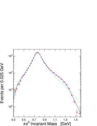
Figure 1: Mass distribution in CLEO $\tau\rightarrow\nu_{\tau}\pi^{-}\pi^{0}$ events. The solid curve overlaid is the result of the Kühn-Santamaria fit, while the dashed curve has the $\rho(1400)$ contribution turned off.

The quality of data on $e^{+}e^{-}\rightarrow\pi^{+}\pi^{-}$ has also recently improved with the release of the CMD-2 results from Novosibirsk [6]. A comparison of the mass spectrum as measured in $e^{+}e^{-}$ and $\tau$ data is given in figure 2 (for this exercise the $\rho-\omega$ interference has to be artificially introduced in the $\tau$ data). Although the agreement looks impressive, it is possible to quantify it by computing a single number, integrating over the complete spectrum. It is convenient for this to use the branching ratio $B(\tau\rightarrow\nu_{\tau}\pi^{-}\pi^{0})$ as directly measured in $\tau$ decays and computed from the $e^{+}e^{-}$ spectral function under the assumption of CVC. Using $B(\tau\rightarrow\nu_{\tau}h^{-}\pi^{0})=(25.79\pm 0.15)\%$ [7] and subtracting out $B(\tau\rightarrow\nu_{\tau}K^{-}\pi^{0})=(0.45\pm 0.02)\%$ [8], one gets $B(\tau\rightarrow\nu_{\tau}\pi^{-}\pi^{0})=(25.34\pm 0.15)\%$, somewhat larger than the CVC value using all available $e^{+}e^{-}$ data, $B^{CVC}_{2\pi}=(24.65\pm 0.35)\%$ [9]. This $1.8\sigma$ discrepancy should be further investigated with a detailed examination of the respective possible systematic effects, such as radiative corrections in $e^{+}e^{-}$ data and $\pi^{0}$ reconstruction in $\tau$ data. CVC violations are of course expected at some point: hadronic violation should be very small ($\sim(m_{u}-m_{d})^{2}/m_{\tau}^{2}$), while significant effects could arise from long-distance radiative processes. Estimates show that the difference between the charged and neutral $\rho$ widths should only be at the level of $(0.3\pm 0.4)\%$ [10].

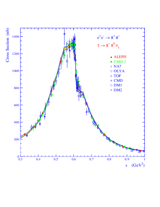
Figure 2: Cross section for $e^{+}e^{-}\rightarrow\pi^{+}\pi^{-}$ compared to the ALEPH $\tau$ data using CVC with $\rho-\omega$ interference built in (shaded band).

The $4\pi$ final states have also been studied [2, 11]. Tests of CVC are severely hampered by large deviations between different $e^{+}e^{-}$ experiments which disagree well beyond their quoted systematic uncertainties. A new CLEO analysis studies the resonant structure in the $3\pi\pi^{0}$ channel which is shown to be dominated by $\omega\pi$ and $a_{1}\pi$ contributions. The $\omega\pi$ spectral function shown in figure 3 is in good agreement with CMD-2 results and it is interpreted by a sum of $\rho$-like amplitudes. The mass of the second state is however found at $(1523\pm 10)$MeV, in contrast with the value $(1406\pm 14)$MeV from the fit of the $2\pi$ spectral function. This point has to be clarified. Following a limit of $8.6\%$ obtained earlier by ALEPH [12], CLEO sets a new $95\%$ CL limit of $6.4\%$ for the relative contribution of second-class currents in the decay $\tau\rightarrow\nu_{\tau}\pi^{-}\omega$ from the hadronic angular decay distribution.

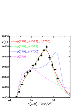
Figure 3: Fits of the CLEO spectral function for $\tau\rightarrow\nu_{\tau}\pi^{-}\omega$.

2.2 Axial-vector states

The decay $\tau\rightarrow\nu_{\tau}3\pi$ is the cleanest place to study axial-vector resonance structure. The spectrum is dominated by the $1^{+}$ $a_{1}$ state, known to decay essentially through $\rho\pi$. A comprehensive analysis of the $\pi^{-}2\pi^{0}$ channel has been presented by CLEO. First, a model-independent determination of the hadronic structure functions gave no evidence for non-axial-vector contributions ($<17\%$ at $90\%$ CL) [13]. Second, a partial-wave amplitude analysis was performed [14]: while the dominant $\rho\pi$ mode was of course confirmed, it came as a surprize that an important contribution ($\sim 20\%$) from scalars ($\sigma$, $f_{0}(1470)$, $f_{2}(1270)$) was found in the $2\pi$ system.

The $a_{1}\rightarrow\pi^{-}2\pi^{0}$ lineshape is displayed in figure 4 where the opening of the $K^{*}K$ decay mode in the total $a_{1}$ width is clearly seen. The derived branching ratio, $B(a_{1}\rightarrow K^{*}K)=(3.3\pm 0.5)\%$ is in good agreement with ALEPH results on the $K\bar{K}\pi$ modes which were indeed shown (with the help of $e^{+}e^{-}$ data and CVC) to be axial-vector ($a_{1}$) dominated with $B(a_{1}\rightarrow K^{*}K)=(2.6\pm 0.3)\%$  [8]. No conclusive evidence for a higher mass state ($a^{\prime}_{1}$) is found in this analysis.

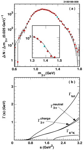
Figure 4: (a) $3\pi$ mass spectrum from CLEO in the $\pi^{-}2\pi^{0}$ channel with the lineshape from the resonance fit (zoom on the $K^{*}K$ threshold). In (b), the $\sqrt{s}$-dependent $a_{1}$ width is plotted with the different contributions considered.

3 Inclusive spectral functions

The $\tau$ nonstrange spectral functions have been measured by ALEPH  [2, 15] and OPAL [16]. The procedure requires a careful separation of vector (V) and axial-vector (A) states involving the reconstruction of multi-$\pi^{0}$ decays and the proper treatment of final states with a $K\bar{K}$ pair. The $V$ and $A$ spectral functions are given in figures 5 and 6, respectively. They show a strong resonant behaviour, dominated by the lowest $\rho$ and $a_{1}$ states, with a tendancy to converge at large mass toward a value near the parton model expectation. Yet, the vector part stays clearly above while the axial-vector one lies below. Thus, the two spectral functions are clearly not ’asymptotic’ at the $\tau$ mass scale.

The $V+A$ spectral function, shown in figure 7 has a clear converging pattern toward a value above the parton level as expected in QCD. In fact, it displays a textbook example of global duality, since the resonance-dominated low-mass region shows an oscillatory behaviour around the asymptotic QCD expectation, assumed to be valid in a local sense only for large masses. This feature will be quantitatively discussed in the next section.

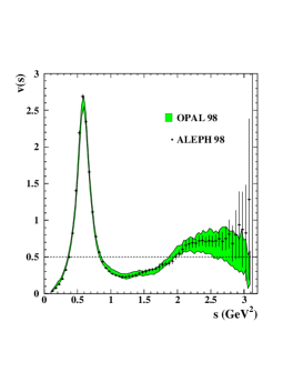
Figure 5: Inclusive nonstrange vector spectral function from ALEPH and OPAL. The dashed line is the expectation from the naive parton model

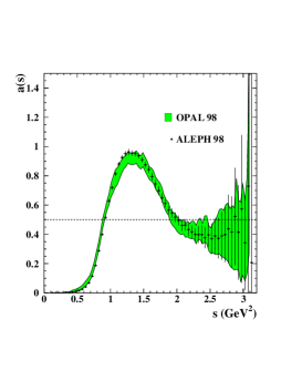
Figure 6: Inclusive nonstrange axial-vector spectral function from ALEPH and OPAL. The dashed line is the expectation from the naive parton model.

Figure 7: Inclusive $V+A$ nonstrange spectral function from ALEPH. The dashed line is the expectation from the naive parton model, while the solid one is from massless perturbative QCD using $\alpha_{s}(M_{\rm Z}^{2})=0.120$.

4 QCD analysis of nonstrange $\tau$ decays

4.1 Motivation

The total hadronic $\tau$ width, properly normalized to the known leptonic width,

$$R_{\tau}=\frac{\Gamma(\tau^{-}\rightarrow{\rm hadrons}^{-}\,\nu_{\tau})}{\Gamma(\tau^{-}\rightarrow e^{-}\,\bar{\nu}_{e}\nu_{\tau})}$$ (3)

should be well predicted by QCD as it is an inclusive observable. Compared to the similar quantity defined in $e^{+}e^{-}$ annihilation, it is even twice inclusive: not only all produced hadronic states at a given mass are summed over, but an integration is performed over all the possible masses from $m_{\pi}$ to $m_{\tau}$.

This favourable situation could be spoiled by the fact that the $Q^{2}$ scale is rather small, so that questions about the validity of a perturbative approach can be raised. At least two levels are to be considered: the convergence of the perturbative expansion and the control of the nonperturbative contributions. Happy circumstances make these contributions indeed very small[17, 18].

4.2 Theoretical prediction for $R_{\tau}$

The imaginary parts of the vector and axial-vector two-point correlation functions $\Pi^{(J)}_{\bar{u}d,V/A}(s)$, with the spin $J$ of the hadronic system, are proportional to the $\tau$ hadronic spectral functions with corresponding quantum numbers. The non-strange ratio $R_{\tau}$ can be written as an integral of these spectral functions over the invariant mass-squared $s$ of the final state hadrons [19]:

$$R_{\tau}(s_{0}) = 12\pi S_{\rm EW}\int\limits_{0}^{s_{0}}\frac{ds}{s_{0}}\left(1-\frac{s}{s_{0}}\right)^{\!\!2}$$

$$\times\left[\left(1+2\frac{s}{s_{0}}\right){\rm Im}\Pi^{(1)}(s+i\epsilon)\,+\,{\rm Im}\Pi^{(0)}(s+i\epsilon)\right]$$

By Cauchy’s theorem the imaginary part of $\Pi^{(J)}$ is proportional to the discontinuity across the positive real axis.

The energy scale $s_{0}$ for $s_{0}=m_{\tau}^{2}$ is large enough that contributions from nonperturbative effects be small. It is therefore assumed that one can use the Operator Product Expansion (OPE) to organize perturbative and nonperturbative contributions [20] to $R_{\tau}(s_{0})$.

The theoretical prediction of the vector and axial-vector ratio $R_{\tau,V/A}$ can thus be written as:

$$R_{\tau,V/A}\;=\;\frac{3}{2}|V_{ud}|^{2}S_{\rm EW}$$

$$\times\left(1+\delta^{(0)}+\delta^{\prime}_{\rm EW}+\delta^{(2-\rm mass)}_{ud,V/A}+\sum_{D=4,6,8}\delta_{ud,V/A}^{(D)}\right)$$

with the residual non-logarithmic electroweak correction $\delta^{\prime}_{\rm EW}=0.0010$ [21], neglected in the following, and the dimension $D=2$ contribution $\delta^{(2-\rm mass)}_{ud,V/A}$ from quark masses which is lower than $0.1\%$ for $u,d$ quarks. The term $\delta^{(0)}$ is the purely perturbative contribution, while the $\delta^{(D)}$ are the OPE terms in powers of $s_{0}^{-D/2}$ of the following form

$$\delta_{ud,V/A}^{(D)}\;\sim\;\sum_{{\rm dim}{\cal O}=D}\frac{\langle{\cal O}_{ud}\rangle_{V/A}}{(-s_{0})^{D/2}}$$ (6)

where the long-distance nonperturbative effects are absorbed into the vacuum expectation elements $\langle{\cal O}_{ud}\rangle$.

The perturbative expansion (FOPT) is known to third order [22]. A resummation of all known higher order logarithmic integrals improves the convergence of the perturbative series (contour-improved method $\rm FOPT_{\rm CI}$} [23]. As some ambiguity persists, the results are given as an average of the two methods with the difference taken as systematic uncertainty.

4.3 Measurements

The ratio $R_{\tau}$ is obtained from measurements of the leptonic branching ratios:

$$R_{\tau} = 3.647\pm 0.014$$ (7)

using a value $B(\tau^{-}\rightarrow e^{-}\,\bar{\nu}_{e}\nu_{\tau})=(17.794\pm 0.045)\%$ which includes the improvement in accuracy provided by the universality assumption of leptonic currents together with the measurements of $B(\tau^{-}\rightarrow e^{-}\,\bar{\nu}_{e}\nu_{\tau})$, $B(\tau^{-}\rightarrow\mu^{-}\,\bar{\nu}_{\mu}\nu_{\tau})$ and the $\tau$ lifetime. The nonstrange part of $R_{\tau}$ is obtained subtracting out the measured strange contribution (see last section).

Two complete analyses of the $V$ and $A$ parts have been performed by ALEPH [15] and OPAL [16]. Both use the world-average leptonic branching ratios, but their own measured spectral functions. The results on $\alpha_{s}(m_{\tau}^{2})$ are therefore strongly correlated and indeed agree when the same theoretical prescriptions are used. Here only the ALEPH results are given.

4.4 Results of the fits

The results of the fits are given in table 1. The limited number of observables and the strong correlations between the spectral moments introduce large correlations, especially between the fitted nonperturbative operators.

ALEPH	$\alpha_{s}(m_{\tau}^{2})$	$\delta_{\rm NP}$
V	$0.330\pm 0.014\pm 0.018$	$0.020\pm 0.004$
A	$0.339\pm 0.013\pm 0.018$	$-0.027\pm 0.0004$
V+A	$0.334\pm 0.007\pm 0.021$	$-0.003\pm 0.0004$

Table 1: Fit results of $\alpha_{s}(m_{\tau}^{2})$ and the OPE nonperturbative contributions from vector, axial-vector and $(V+A)$ combined fits using the corresponding ratios $R_{\tau}$ and the spectral moments as input parameters. The second error is given for theoretical uncertainty.

One notices a remarkable agreement within statistical errors between the $\alpha_{s}(m_{\tau}^{2})$ values using vector and axial-vector data. The total nonperturbative power contribution to $R_{\tau,V+A}$ is compatible with zero within an uncertainty of 0.4$\%$, that is much smaller than the error arising from the perturbative term. This cancellation of the nonperturbative terms increases the confidence on the $\alpha_{s}(m_{\tau}^{2})$ determination from the inclusive $(V+A)$ observables.

The final result is :

$$\alpha_{s}(m_{\tau}^{2})=0.334\pm 0.007_{\rm exp}\pm 0.021_{\rm th}$$ (8)

where the first error accounts for the experimental uncertainty and the second gives the uncertainty of the theoretical prediction of $R_{\tau}$ and the spectral moments as well as the ambiguity of the theoretical approaches employed.

4.5 Test of the running of $\alpha_{s}(s)$ at low energies

Using the spectral functions, one can simulate the physics of a hypothetical $\tau$ lepton with a mass $\sqrt{s_{0}}$ smaller than $m_{\tau}$ through equation (4.2) and hence further investigate QCD phenomena at low energies. Assuming quark-hadron duality, the evolution of $R_{\tau}(s_{0})$ provides a direct test of the running of $\alpha_{s}(s_{0})$, governed by the RGE $\beta$-function. On the other hand, it is a test of the validity of the OPE approach in $\tau$ decays.

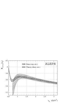
Figure 8: The ratio $R_{\tau,V+A}$ versus the square “$\tau$ mass” $s_{0}$. The curves are plotted as error bands to emphasize their strong point-to-point correlations in $s_{0}$. Also shown is the theoretical prediction using the results of the fit at $s_{0}=m_{\tau}^{2}$.

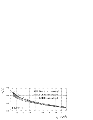
Figure 9: The running of $\alpha_{s}(s_{0})$ obtained from the fit of the theoretical prediction to $R_{\tau,V+A}(s_{0})$. The shaded band shows the data including experimental errors. The curves give the four-loop RGE evolution for two and three flavours.

The functional dependence of $R_{\tau,V+A}(s_{0})$ is plotted in figure 8 together with the theoretical prediction using the results of table 1. Below $1~{}{\rm GeV}^{2}$ the error of the theoretical prediction of $R_{\tau,V+A}(s_{0})$ starts to blow up due to the increasing uncertainty from the unknown fourth-order perturbative term. Figure 9 shows the plot corresponding to Fig. 8, translated into the running of $\alpha_{s}(s_{0})$, i.e., the experimental value for $\alpha_{s}(s_{0})$ has been individually determined at every $s_{0}$ from the comparison of data and theory. Good agreement is observed with the four-loop RGE evolution using three quark flavours.

The experimental fact that the nonperturbative contributions cancel over the whole range $1.2~{}{\rm GeV}^{2}\leq s_{0}\leq m_{\tau}^{2}$ leads to confidence that the $\alpha_{s}$ determination from the inclusive $(V+A)$ data is robust.

4.6 Discussion on the determination of $\alpha_{s}(m_{\tau}^{2})$

The evolution of the $\alpha_{s}(m_{\tau}^{2})$ measurement from the inclusive $(V+A)$ observables based on the Runge-Kutta integration of the differential equation of the renormalization group to N³LO [24, 26] yields

$$\alpha_{s}(M_{\rm Z}^{2})=\\ 0.1202\pm 0.0008_{\rm exp}\pm 0.0024_{\rm th}\pm 0.0010_{\rm evol}$$

where the last error stands for possible ambiguities in the evolution due to uncertainties in the matching scales of the quark thresholds [26].

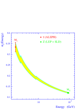
Figure 10: Evolution of the strong coupling measured at $m_{\tau}^{2})$ to $M_{Z}^{2}$ predicted by QCD compared to the direct measurement. The evolution is carried out at 4 loops, while the flavour matching is accomplished at 3 loops at $2~{}m_{c}$ and $2~{}m_{b}$ thresholds.

The result (4.6) can be compared to the determination from the global electroweak fit. The variable $R_{Z}$ has similar advantages as $R_{\tau}$, but it differs concerning the convergence of the perturbative expansion because of the much larger scale. It turns out that this determination is dominated by experimental errors with very small theoretical uncertainties, i.e. the reverse of the situation encountered in $\tau$ decays. The most recent value[27] yields $\alpha_{s}(M_{\rm Z}^{2})=0.119\pm 0.003$, in excellent agreement with (4.6). Fig. 10 illustrates well the agreement between the evolution of $\alpha_{s}(m_{\tau}^{2})$ predicted by QCD and $\alpha_{s}(M_{\rm Z}^{2})$.

5 Applications to hadronic vacuum polarization

5.1 Improvements to the standard calculations

From the studies presented above we have learned that:

• the $I=1$ vector spectral function from $\tau$ decays agrees with that from $e^{+}e^{-}$ annihilation, while it is more precise for masses less than $1.6$ GeV as can be seen on figure 11. Small CVC violations are expected at a few $10^{-3}$ level [10] from radiative $\rho$ decays and SU(2)-breaking in the $\pi$ and $\rho$ masses.

• the description of $R_{\tau}$ by perturbative QCD works down to a scale of $1$ GeV. Nonperturbative contributions at $1.8~{}GeV$ are well below 1 % in this case. They are larger ($\sim 3$ %) for the vector part alone, but reasonably well described by OPE. The complete (perturbative + nonperturbative) description is accurate at the 1 % level at $1.8$ GeV for integrals over the vector spectral function  such as $R_{\tau,V}$.

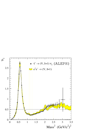
Figure 11: Global test of CVC using $\tau$ and $e^{+}e^{-}$ vector spectral functions.

These two facts have direct applications to calculations of hadronic vacuum polarisation which involve the knowledge of the vector spectral function: the muon magnetic anomaly and the running of $\alpha$. In both cases, the standard method involves a dispersion integral over the vector spectral function taken from the $e^{+}e^{-}~{}\rightarrow$ hadrons data. Eventually at large energies, QCD is used to replace experimental data. Hence the precision of the calculation is given by the accuracy of the data, which is poor above $1.5$ GeV. Even at low energies, the precision can be significantly improved at low masses by using $\tau$ data [10].

The next breakthrough comes about using the prediction of perturbative QCD far above quark thresholds, but at low enough energies (compatible with the remarks above) in place of noncompetitive experimental data[28]. This procedure involves a proper treatment of the quark masses in the QCD prediction[25].

Finally, it is still possible to improve the contributions from data by using analyticity and QCD sum rules, basically without any additional assumption. This idea, advocated in Ref. [29], has been used within the procedure described above to still improve the calculations [30].

The experimental results of $R(s)$ and the theoretical prediction are shown in figure 12. The shaded bands depict the regions where data are used instead of theory to evaluate the respective integrals. Good agreement between data and QCD is found above 8 GeV, while at lower energies systematic deviations are observed. The $R$ measurements in this region are essentially provided by the $\gamma\gamma 2$ [31] and MARK I [32] collaborations. MARK I data above 5 GeV lie systematically above the measurements of the Crystal Ball [33] and MD1 [34] Collaborations as well as the QCD prediction.

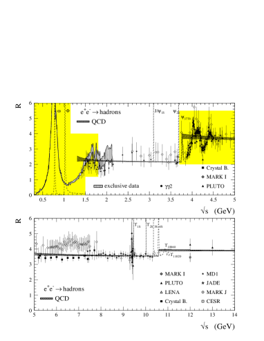
Figure 12: Inclusive hadronic cross section ratio in $e^{+}e^{-}$ annihilation versus the c.m. energy $\sqrt{s}$. Additionally shown is the QCD prediction of the continuum contribution from Ref. [28] as explained in the text. The shaded areas depict regions were experimental data are used for the evaluation of $\Delta\alpha_{\rm had}(M_{\rm Z}^{2})$ and $a_{\mu}^{\rm had}$ in addition to the measured narrow resonance parameters. The exclusive $e^{+}e^{-}$ cross section measurements at low c.m. energies are taken from DM1,DM2,M2N,M3N,OLYA,CMD,ND and $\tau$ data from ALEPH (see Ref. [10] for detailed information).

5.2 Muon magnetic anomaly

By virtue of the analyticity of the vacuum polarization correlator, the contribution of the hadronic vacuum polarization to $a_{\mu}$ can be calculated via the dispersion integral [35]

$$a_{\mu}^{\mathrm{h}ad}\>=\>\frac{1}{4\pi^{3}}\int\limits_{4m_{\pi}^{2}}^{\infty}ds\,\sigma_{\mathrm{h}ad}(s)\,K(s)$$ (9)

Here $\sigma_{\mathrm{h}ad}(s)$ is the total $e^{+}e^{-}$$\rightarrow\,$hadrons cross section as a function of the c.m. energy-squared $s$, and $K(s)$ denotes a well-known QED kernel.

The function $K(s)$ decreases monotonically with increasing $s$. It gives a strong weight to the low energy part of the integral (9). About 91$\%$ of the total contribution to $a_{\mu}^{\rm had}$ is accumulated at c.m. energies $\sqrt{s}$ below 2.1 GeV while 72$\%$ of $a_{\mu}^{\rm had}$ is covered by the two-pion final state which is dominated by the $\rho(770)$ resonance. The new information provided by the ALEPH 2- and 4-pion spectral functions can significantly improve the $a_{\mu}^{\rm had}$ determination.

5.3 Running of the electromagnetic coupling

In the same spirit we evaluate the hadronic contribution $\Delta\alpha(s)$ to the renormalized vacuum polarization function $\Pi_{\gamma}^{\prime}(s)$ which governs the running of the electromagnetic coupling $\alpha(s)$. With $\Delta\alpha(s)$=$-4\pi\alpha\,{\mathrm{R}e}\left[\Pi_{\gamma}^{\prime}(s)-\Pi_{\gamma}^{\prime}(0)\right]$, one has

$$\alpha(s)\>=\>\frac{\alpha(0)}{1-\Delta\alpha(s)}$$ (10)

where $4\pi\alpha(0)$ is the square of the electron charge in the long-wavelength Thomson limit.

The leading order leptonic contribution is equal to $314.2\times 10^{-4}$. Using analyticity and unitarity, the dispersion integral for the contribution from the light quark hadronic vacuum polarization $\Delta\alpha_{\rm had}(M_{\rm Z}^{2})$ reads [36]

$$\Delta\alpha_{\mathrm{h}ad}^{(5)}(M_{\mathrm{Z}}^{2})\>=\>\\ -\frac{M_{\mathrm{Z}}^{2}}{4\pi^{2}\,\alpha}\,{\mathrm{R}e}\int\limits_{4m_{\pi}^{2}}^{\infty}ds\,\frac{\sigma_{\mathrm{h}ad}(s)}{s-M_{\mathrm{Z}}^{2}-i\epsilon}$$

where $\sigma(s)=16\pi^{2}\alpha^{2}(s)/s\cdot{\mathrm{I}m}\Pi_{\gamma}^{\prime}(s)$ from the optical theorem. In contrast to $a_{\mu}^{\rm had}$, the integration kernel favours cross sections at higher masses. Hence, the improvement when including $\tau$ data is expected to be small.

The top quark contribution can be calculated using the next-to-next-to-leading order $\alpha_{s}^{3}$ prediction of the total inclusive cross section ratio $R$ from perturbative QCD [22, 37]. The evaluation of the integral (5.3) with $m_{\mathrm{t}op}=175$ GeV yields $\Delta\alpha_{\mathrm{t}op}(M_{\mathrm{Z}}^{2})=-0.6\times 10^{-4}$.

5.4 Results

The combination of the theoretical and experimental evaluations of the integrals (5.3) and (9) yields the results

$$\Delta\alpha_{\rm had}(M_{\rm Z}^{2}) = (276.3\pm 1.1_{\rm exp}\pm 1.1_{\rm th})\times 10^{-4}$$

$$\alpha^{-1}(M_{\rm Z}^{2}) = 128.933\pm 0.015_{\rm exp}\pm 0.015_{\rm th}$$

$$a_{\mu}^{\rm had} = (692.4\pm 5.6_{\rm exp}\pm 2.6_{\rm th})\times 10^{-10}$$

$$a_{\mu}^{\rm SM} = (11\,659\,159.6$$ (11)

$$\pm 5.6_{\rm exp}\pm 3.7_{\rm th})\times 10^{-10}$$

and $a_{e}^{\rm had}=(187.5\pm 1.7_{\rm exp}\pm 0.7_{\rm th})\times 10^{-14}$ for the leading order hadronic contribution to $a_{e}$. The total $a_{\mu}^{\rm SM}$ value includes additional contributions from non-leading order hadronic vacuum polarization (summarized in Refs.[38, 10]) and light-by-light scattering [39, 40] contributions. Figures 13 and 14 show a compilation of published results for the hadronic contributions to $\alpha(M_{\rm Z}^{2})$ and $a_{\mu}$. Some authors give the hadronic contribution for the five light quarks only and add the top quark part separately. This has been corrected for in Fig. 13.

Figure 13: Comparison of $\Delta\alpha_{\rm had}(M_{\rm Z}^{2})$ evaluations. The values are taken from Refs. [41, 37, 42, 43, 44, 10, 28, 45, 46, 30].

Figure 14: Comparison of $a_{\mu}^{\rm had}$ evaluations. The values are taken from Refs. [47, 48, 49, 37, 50, 10, 28, 30].

5.5 Outlook

These results have direct implications for phenomenology and on-going experimental programs.

Most of the sensitivity to the Higgs boson mass originates from the measurements of asymmetries in the process $e^{+}e^{-}\rightarrow Z\rightarrow$ fermion pairs and in fine from $(sin^{2}\theta_{W})_{eff}=\bar{s}^{2}$. Unfortunately, this approach is limited by the fact that the intrinsic uncertainty on $\alpha(M_{\rm Z}^{2})$ in the standard evaluation is at the same level as the experimental accuracy on $\bar{s}^{2}$. The situation has completely changed with the new determination of $\alpha(M_{\rm Z}^{2})$ which does not limit anymore the adjustment of the Higgs mass from accurate experimental determinations of ${\rm sin}^{2}\theta_{\rm W}$. The improvement in precision can be directly appreciated on the relevant variable $log~{}M_{H}$ with $M_{H}$ in ${\rm GeV}/c^{2}$ [27]:

$$log~{}M_{H} = 1.88^{+0.31}_{-0.39}$$ (12)

with the ’standard’ $\alpha(M_{Z}^{2})$ [37], and

$$log~{}M_{H} = 1.97^{+0.22}_{-0.25}$$ (13)

with the QCD-improved value [30].

The interest in reducing the uncertainty in the hadronic contribution to $a_{\mu}^{\rm had}$ is directly linked to the possibility of measuring the weak contribution:

$$a_{\mu}^{\mathrm{S}M}\>=\>a_{\mu}^{\mathrm{Q}ED}+a_{\mu}^{\mathrm{h}ad}+a_{\mu}^{\mathrm{w}eak}$$ (14)

where $a_{\mu}^{\mathrm{Q}ED}=(11\,658\,470.6\,\pm\,0.2)\times 10^{-10}$ is the pure electromagnetic contribution (see [51] and references therein), $a_{\mu}^{\rm had}$ is the contribution from hadronic vacuum polarization, and $a_{\mu}^{\mathrm{w}eak}=(15.1\,\pm\,0.4)\times 10^{-10}$ [51, 52, 53] accounts for corrections due to the exchange of the weak interacting bosons up to two loops. The present value from the combined $\mu^{+}$ and $\mu^{-}$ measurements [54],

$$a_{\mu}\>=\>(11\,659\,230\pm 85)\times 10^{-10}$$ (15)

should be improved to a precision of at least $4\times 10^{-10}$ by a forthcoming Brookhaven experiment (BNL-E821) [55], well below the expected weak contribution. Such a programme makes sense only if the uncertainty on the hadronic term is made sufficiently small. The improvements described above represent a significant step in this direction.

6 Strange $\tau$ decays and $m_{s}$

6.1 The strange hadronic decay ratio $R_{\tau,S}$

As previously demonstrated in Ref. [56], the inclusive $\tau$ decay ratio into strange hadronic final states,

$$R_{\tau,S}=\frac{\Gamma(\tau^{-}\rightarrow{\rm hadrons}_{S=-1}^{-}\,\nu_{\tau})}{\Gamma(\tau^{-}\rightarrow e^{-}\,\bar{\nu}_{e}\nu_{\tau})}$$ (16)

can be used due to its precise theoretical prediction [19, 57] to determine $m_{s}(s)$ at the scale $s=M_{\tau}^{2}$. Since then it was shown [58] that the perturbative expansion used for the massive term in Ref. [57] was incorrect. After correction the series shows a problematic convergence behaviour [58, 59, 60].

Figure 15: Some of the new ALEPH results on decay modes with kaons compared to the published data.

Similarly to the nonstrange case, the QCD prediction is given by equations (4.2) and (4.2) where the attention is now turned to the $\delta^{(2-\rm mass)}$ term, important for the relatively heavy strange quark. The corresponding perturbative expansion is known to second order for the $J=1+0$ part and to the third order for $J=0$ [57, 58]. While the $J=1+0$ series behaves well, the $J=0$ expansion in fact diverges after the second term.

Following these observations, two methods can be considered in order to determine $m_{s}(m_{\tau}^{2})$:

• in the inclusive method, the inclusive strange hadronic rate is considered and both $J=1+0$ and $J=0$ are included with their respective convergence behaviour taken into account in the theoretical uncertainties.

• the ‘1+0’ method singles out the well-behaved $J=1+0$ part by subtracting the experimentally determined $J=0$ longitudinal component from data. The measurement is then less inclusive and the sensitivity to $m_{s}$ is significantly reduced; however, the $\delta_{2}$ perturbative expansion is under control and the corresponding theoretical uncertainty is reduced.

6.1.1 New ALEPH results on strange decays

ALEPH has recently published a comprehensive study of $\tau$ decay modes including kaons (charged, $K^{0}_{S}$ and $K^{0}_{L}$) [61, 62, 63, 8] up to four hadrons in the final state. A comparison with the published results is given in figure 15.

The total branching ratio for $\tau$ into strange final states, $B_{S}$, is

$$B_{S}=(2.87\pm 0.12)\%$$ (17)

corresponding to

$$R_{\tau,S}=0.1610\pm 0.0066$$ (18)

Since the QCD expectation for a massless quarks is $0.1809\pm 0.0036$, the result (18) is evidence for a massive $s$ quark.

The strange spectral function is given in figure 16, dominated at low mass by the $K^{*}$ resonance.

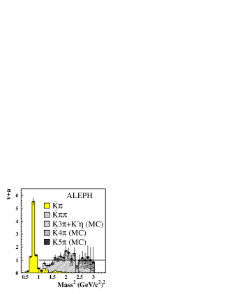
Figure 16: The strange spectral function measured by ALEPH.

6.1.2 The ALEPH analysis for $m_{s}$

As proposed in Ref. [64] and successfully applied in $\alpha_{s}(m_{\tau}^{2})$ analyses, the spectral function is used to construct moments

$$R_{\tau,S}^{kl}\;\equiv\;\int\limits_{0}^{M_{\tau}^{2}}ds\,\left(1-\frac{s}{M_{\tau}^{2}}\right)^{\!\!k}\left(\frac{s}{M_{\tau}^{2}}\right)^{\!\!l}\frac{dR_{\tau,S}}{ds}$$ (19)

In order to reduce the theoretical uncertainties one considers the difference between non-strange and strange spectral moments, properly normalized with their respective CKM matrix elements:

$$\Delta_{\tau}^{kl}\;\equiv\;\frac{1}{|V_{ud}|^{2}}R_{\tau,S=0}^{kl}-\frac{1}{|V_{us}|^{2}}R_{\tau,S=-1}^{kl}$$ (20)

for which the massless perturbative contribution vanishes so that the theoretical prediction now reads (setting $m_{u}=m_{d}=0$)

$$\Delta_{\tau}^{kl}\;=\;3S_{\rm EW}\left(-\,\delta_{S}^{kl(2-\rm mass)}+\sum_{D=4,6,\dots}\tilde{\delta}^{kl(D)}\right)$$ (21)

For the CKM matrix elements the values $|V_{ud}|=0.9751\pm 0.0004$ and $|V_{us}|=0.2218\pm 0.0016$ [65] are used, while the errors are included in the theoretical uncertainties.

Figure 17 shows the weighted integrand of the lowest moment $\Delta^{00}_{\tau}$ from the ALEPH data, as a function of the invariant mass-squared, and for which the expectation from perturbative QCD vanishes.

Figure 17: Integrand of Eq. (20) for (k=0, l=0), $i.e.$, difference of the Cabibbo corrected non-strange and strange invariant mass spectra.

Subtracting out the experimental $J=0$ contribution (essentially given by the single K channel), a fit to 5 moments is performed with the safer $J=1+0$ method, yielding

$$m_{s}(m_{\tau}^{2}) = (176^{\,+37_{\rm exp}+24_{\rm th}}_{\,-48_{\rm exp}-28_{\rm th}})~{}{\rm MeV}/c^{2}$$ (22)

$$\tilde{\delta}^{(6)} = 0.039\pm 0.016_{\rm exp}\pm 0.014_{\rm th}$$ (23)

$$\tilde{\delta}^{(8)} = -0.021\pm 0.014_{\rm exp}\pm 0.008_{\rm th}$$ (24)

with additional (smaller) uncertainties from the fitting procedure and the determination of the $J=0$ part. The quoted theoretical errors are mostly from the $V_{us}$ uncertainty. The $D=6$ and $D=8$ strange contributions are found to be surprizingly larger than their nonstrange counterparts. If the fully inclusive method is used instead (with the problematic convergence) the result $m_{s}(m_{\tau}^{2})=(149^{\,+24_{\rm exp}+21_{\rm th}}_{\,-30_{\rm exp}-25_{\rm th}})~{}{\rm MeV}/c^{2}$ is obtained.

The result (22) can be evolved to the scale of 1 GeV using the four-loop RGE $\gamma$-function [66], yielding

$$m_{s}(1~{}{\rm GeV}^{2})=(234^{\,+61}_{\,-76})~{}{\rm MeV}/c^{2}$$ (25)

This value of $m_{s}$ is somewhat larger than previous determinations [67], but consistent with them within errors.

7 Conclusions

The decays $\tau\rightarrow\nu_{\tau}$ + hadrons constitute a clean and powerful way to study hadronic physics up to $\sqrt{s}\sim 1.8$ GeV. Beautiful resonance analyses have already been done, providing new insight into hadron dynamics. Probably the major surprize has been the fact that inclusive hadron production is well described by perturbative QCD with very small nonperturbative components at the $\tau$ mass. Despite the fact that this low-energy region is dominated by resonance physics, methods based on global quark-hadron duality work indeed very well.

The measurement of the vector and axial-vector spectral functions has provided the way for quantitative analyses. Precise determinations of $\alpha_{s}$ agree for both spectral functions and they also agree with all the other determinations from the Z width, the rate of Z to jets and deep inelastic lepton scattering. Indeed from $\tau$ decays

$$\alpha_{s}(M_{\rm Z}^{2})_{\tau}=0.1202\pm 0.0027$$ (26)

in excellent agreement with the average from all other determinations [68]

$$\alpha_{s}(M_{\rm Z}^{2})_{non-\tau}=0.1187\pm 0.0020$$ (27)

The use of the vector $\tau$ spectral function and the QCD-based approach as tested in $\tau$ decays improve the calculations of hadronic vacuum polarization considerably. Significant results have been obtained for the running of $\alpha$ to the Z mass and the muon anomalous magnetic moment. Both of these quantities must be known with high precision as they give access to new physics.

Finally the strange spectral function has been measured, providing a determination of the strange quark mass.

- [1] W. Marciano and A. Sirlin, Phys. Rev. Lett. 61(1988)1815.
- [2] R. Barate et al. (ALEPH Collaboration), Z. Phys. C76 (1997) 15.
- [3] S. Anderson et al. (CLEO Collaboration), hep-ex/9910046.
- [4] G.J. Gounaris and J.J. Sakurai, Phys. Rev. Lett. 21 (1968) 244.
- [5] J.H. Kühn and A. Santamaria, Z. Phys. C48 (1990) 445.
- [6] R.R. Akhmetshin et al., hep-ex/9904027.
- [7] B.K. Heltsley, Nucl. Phys. B (Proc. Suppl.) 64 (1998) 391.
- [8] ALEPH Collaboration, hep-ex/9903015.
- [9] S.I. Eidelman, Workshop on Lepton Moments, Heidelberg (June 10-12 1999).
- [10] R. Alemany, M. Davier and A. Höcker, Europ. Phys. J. C2 (1998) 123.
- [11] K.W. Edwards et al. (CLEO Collaboration), hep-ex/9908024.
- [12] D. Buskulic et al. (ALEPH Collaboration), Z. Phys. C74 (1997) 263.
- [13] T.E. Browder et al. (CLEO Collaboration), hep-ex/9908030.
- [14] D.M. Asner et al. (CLEO Collaboration), CLNS 99/1635, CLEO 99-13.
- [15] ALEPH Collaboration, Eur.Phys.J. C4 (1998) 409.
- [16] OPAL Collaboration, CERN-EP/98-102, June 1998.
- [17] E. Braaten, Phys. Rev. Lett./ 60 (1988) 1606.
- [18] S. Narison and A. Pich, Phys. Lett./ B211 (1988) 183.
- [19] E. Braaten, S. Narison and A. Pich, Nucl. Phys. B373 (1992) 581.
- [20] M.A. Shifman, A.L. Vainshtein and V.I. Zakharov, Nucl. Phys. B147 (1979) 385, 448, 519.
- [21] E. Braaten and C.S. Li, Phys. Rev. D42 (1990) 3888.
- [22] L.R. Surguladze and M.A. Samuel, Phys. Rev. Lett. 66 (1991) 560; S.G. Gorishny, A.L. Kataev and S.A. Larin, Phys. Lett. B259 (1991) 144.
- [23] F. Le Diberder and A. Pich, Phys. Lett. B286 (1992) 147.
- [24] S.A. Larin, T. van Ritbergen and J.A.M. Vermaseren, Phys. Lett. B400 (1997) 379; K.G. Chetyrkin, B.A. Kniehl and M. Steinhauser, Nucl. Phys. B510 (1998) 61; W. Bernreuther, W. Wetzel, Nucl. Phys. B197 (1982) 228; W. Wetzel, Nucl. Phys. B196 (1982) 259; W. Bernreuther, PITHA-94-31 (1994).
- [25] K.G. Chetyrkin, B.A. Kniehl and M. Steinhauser, Phys. Rev. Lett. 79 (1997) 2184;
- [26] G. Rodrigo, A. Pich, A. Santamaria, FTUV-97-80 (1997).
- [27] A. Blondel, in Rencontres de Blois Frontiers of Matter, Blois (June 28-July 3 1999).
- [28] M. Davier and A. Höcker, Phys. Lett. B419 (1998) 419.
- [29] S. Groote, J.G. Körner, N.F. Nasrallah and K. Schilcher, Report MZ-TH-98-02 (1998).
- [30] M. Davier and A. Höcker, Phys. Lett. B435 (1998) 427.
- [31] C. Bacci et al. ( Collaboration), Phys. Lett. B86 (1979) 234.
- [32] J.L. Siegrist et al. (MARK I Collaboration), Phys. Rev. D26 (1982) 969.
- [33] Z. Jakubowski et al. (Crystal Ball Collaboration), Z. Phys. C40 (1988) 49; C. Edwards et al. (Crystal Ball Collaboration), SLAC-PUB-5160 (1990).
- [34] A.E. Blinov et al. (MD-1 Collaboration), Z. Phys. C49 (1991) 239; A.E. Blinov et al. (MD-1 Collaboration), Z. Phys. C70 (1996) 31.
- [35] M. Gourdin and E. de Rafael, Nucl. Phys. B10 (1969) 667; S.J. Brodsky and E. de Rafael, Phys. Rev. 168 (1968) 1620.
- [36] N. Cabibbo and R. Gatto, Phys. Rev. Lett. 4 (1960) 313; Phys. Rev. 124 (1961) 1577.
- [37] S. Eidelman and F. Jegerlehner, Z. Phys. C67 (1995) 585.
- [38] B. Krause, Phys. Lett. B390 (1997) 392.
- [39] M. Hayakawa, T. Kinoshita, Phys. Rev. D57 (1998) 465.
- [40] J. Bijnens, E. Pallante and J. Prades, Nucl. Phys. B474 (1996) 379.
- [41] B.W. Lynn, G. Penso and C. Verzegnassi, Phys. Rev. D35 (1987) 42.
- [42] H. Burkhardt and B. Pietrzyk, Phys. Lett. B356 (1995) 398.
- [43] A.D. Martin and D. Zeppenfeld, Phys. Lett. B345 (1995) 558.
- [44] M.L. Swartz, Phys. Rev. D53 (1996) 5268.
- [45] J.H. Kühn and M. Steinhauser, MPI-PHT-98-12 (1998).
- [46] J. Erler, UPR-796-T, 1998.
- [47] L.M. Barkov et al. (OLYA, CMD Collaboration), Nucl. Phys. B256 (1985) 365.
- [48] T. Kinoshita, B. Nižić and Y. Okamoto, Phys. Rev. D31 (1985) 2108.
- [49] J.A. Casas, C. López and F.J. Ynduráin, Phys. Rev. D32 (1985) 736.
- [50] D.H. Brown and W.A. Worstell, Phys. Rev. D54 (1996) 3237.
- [51] A. Czarnecki, B. Krause and W.J. Marciano, Phys. Rev. Lett. 76 (1995) 3267; Phys. Rev. D52 (1995) 2619.
- [52] T.V. Kukhto, E.A. Kuraev, A. Schiller and Z.K. Silagadze, Nucl. Phys. B371 (1992) 567.
- [53] R. Jackiw and S. Weinberg, Phys. Rev. D5 (1972) 2473.
- [54] J. Bailey et al., Phys. Lett. B68 (1977) 191; F.J.M. Farley and E. Picasso, Advanced Series on Directions in High Energy Physics - Vol. 7 Quantum Electrodynamics, ed. T. Kinoshita, World Scientific 1990.
- [55] B. Lee Roberts, Z. Phys. C56 (Proc. Suppl.) (1992) 101.
- [56] M. Davier, Nucl. Phys. C (Proc. Suppl.) 55 (1997) 395; S.M. Chen, Nucl. Phys. B (Proc. Suppl.) 64 (1998) 265; S.M. Chen, M. Davier and A. Höcker, Nucl. Phys. B (Proc. Suppl.) 76 (1999) 369.
- [57] K.G. Chetyrkin and A. Kwiatkowski, Z. Phys. C59 (1993) 525.
- [58] K. Maltman, hep-ph/9804298.
- [59] A. Pich and J. Prades, hep-ph/9804462.
- [60] K.G. Chetyrkin, J.H. Kühn and A.A. Pivovarov, hep-ph/9805335.
- [61] ALEPH Collaboration, Eur. Phys. J. C1 (1998) 65.
- [62] ALEPH Collaboration, Eur. Phys. J. C4 (1998) 29.
- [63] ALEPH Collaboration, hep-ex/9903014.
- [64] F. Le Diberder and A. Pich, Phys. Lett. B289 (1992) 165.
- [65] R.M. Barnett et al., Particle Data Group, Eur. Phys. J. C3 (1998) 1.
- [66] S.A. Larin, T. van Ritbergen and J.A.M. Vermaseren, Phys. Lett. B405 (1997) 327.
- [67] J. Gasser and H. Leutwyler, Phys. Rep. 87 (1982) 77; M. Jamin and M. Münz, Z. Phys. C66 (1995) 633; K.G. Chetyrkin et al., Phys. Lett. B404 (1997) 337; C. Becchi et al., Z. Phys. C8 (1981) 335; C.A. Dominguez and E. de Rafael, Ann. Phys. 174 (1987) 372; C.A. Dominguez et al., Phys. Lett. B253 (1991) 241; M. Jamin, Nucl. Phys. B (Proc. Suppl.) 64 (1998) 250; A.L. Kataev et al., Nuovo. Cim. A76 (1983) 723; P. Colangelo et al., Phys. Lett. B408 (1997) 340; S. Narison, Phys. Lett. B216 (1989) 191; K.G. Chetyrkin et al., Phys. Rev. D51 (1995) 5090; S. Narison, Phys. Lett. B358 (1995) 113; K. Maltman, Phys. Lett. B428 (1998) 179; C.R. Allton et al., Nucl. Phys. B431 (1994) 667; R. Gupta and T. Bhattacharya, Phys. Rev. D55 (1997) 7203; N. Eicker et al., SESAM-Collaboration, hep-lat/9704019; B.J. Gough et al., Phys. Rev. Lett. 79 (1994) 1662.
- [68] M. Davier, ’98 Renc. Moriond on Electroweak Interactions, Ed. J. Trân Thanh Vân, Frontières, Paris (1998).