Hadronic Structure in the Decay $\tau^{-}\rightarrow\pi^{-}\pi^{0}\nu_{\tau}$

Abstract

We report on a study of the invariant mass spectrum of the hadronic system in the decay $\tau^{-}\to\pi^{-}\pi^{0}\nu_{\tau}$. This study was performed with data obtained with the CLEO II detector operating at the CESR $e^{+}e^{-}$ collider. We present fits to phenomenological models in which resonance parameters associated with the $\rho(770)$ and $\rho(1450)$ mesons are determined. The $\pi^{-}\pi^{0}$ spectral function inferred from the invariant mass spectrum is compared with data on $e^{+}e^{-}\to\pi^{+}\pi^{-}$ as a test of the Conserved Vector Current theorem. We also discuss the implications of our data with regard to estimates of the hadronic contribution to the muon anomalous magnetic moment.

S. Anderson,¹ V. V. Frolov,¹ Y. Kubota,¹ S. J. Lee,¹ R. Mahapatra,¹ J. J. O’Neill,¹ R. Poling,¹ T. Riehle,¹ A. Smith,¹ S. Ahmed,² M. S. Alam,² S. B. Athar,² L. Jian,² L. Ling,² A. H. Mahmood,^2, M. Saleem,² S. Timm,² F. Wappler,² A. Anastassov,³ J. E. Duboscq,³ K. K. Gan,³ C. Gwon,³ T. Hart,³ K. Honscheid,³ H. Kagan,³ R. Kass,³ J. Lorenc,³ H. Schwarthoff,³ E. von Toerne,³ M. M. Zoeller,³ S. J. Richichi,⁴ H. Severini,⁴ P. Skubic,⁴ A. Undrus,⁴ M. Bishai,⁵ S. Chen,⁵ J. Fast,⁵ J. W. Hinson,⁵ J. Lee,⁵ N. Menon,⁵ D. H. Miller,⁵ E. I. Shibata,⁵ I. P. J. Shipsey,⁵ Y. Kwon,^6, A.L. Lyon,⁶ E. H. Thorndike,⁶ C. P. Jessop,⁷ H. Marsiske,⁷ M. L. Perl,⁷ V. Savinov,⁷ D. Ugolini,⁷ X. Zhou,⁷ T. E. Coan,⁸ V. Fadeyev,⁸ I. Korolkov,⁸ Y. Maravin,⁸ I. Narsky,⁸ R. Stroynowski,⁸ J. Ye,⁸ T. Wlodek,⁸ M. Artuso,⁹ R. Ayad,⁹ E. Dambasuren,⁹ S. Kopp,⁹ G. Majumder,⁹ G. C. Moneti,⁹ R. Mountain,⁹ S. Schuh,⁹ T. Skwarnicki,⁹ S. Stone,⁹ A. Titov,⁹ G. Viehhauser,⁹ J.C. Wang,⁹ A. Wolf,⁹ J. Wu,⁹ S. E. Csorna,¹⁰ K. W. McLean,¹⁰ S. Marka,¹⁰ Z. Xu,¹⁰ R. Godang,¹¹ K. Kinoshita,^11, I. C. Lai,¹¹ S. Schrenk,¹¹ G. Bonvicini,¹² D. Cinabro,¹² R. Greene,¹² L. P. Perera,¹² G. J. Zhou,¹² S. Chan,¹³ G. Eigen,¹³ E. Lipeles,¹³ M. Schmidtler,¹³ A. Shapiro,¹³ W. M. Sun,¹³ J. Urheim,¹³ A. J. Weinstein,¹³ F. Würthwein,¹³ D. E. Jaffe,¹⁴ G. Masek,¹⁴ H. P. Paar,¹⁴ E. M. Potter,¹⁴ S. Prell,¹⁴ V. Sharma,¹⁴ D. M. Asner,¹⁵ A. Eppich,¹⁵ J. Gronberg,¹⁵ T. S. Hill,¹⁵ D. J. Lange,¹⁵ R. J. Morrison,¹⁵ T. K. Nelson,¹⁵ R. A. Briere,¹⁶ B. H. Behrens,¹⁷ W. T. Ford,¹⁷ A. Gritsan,¹⁷ H. Krieg,¹⁷ J. Roy,¹⁷ J. G. Smith,¹⁷ J. P. Alexander,¹⁸ R. Baker,¹⁸ C. Bebek,¹⁸ B. E. Berger,¹⁸ K. Berkelman,¹⁸ F. Blanc,¹⁸ V. Boisvert,¹⁸ D. G. Cassel,¹⁸ M. Dickson,¹⁸ P. S. Drell,¹⁸ K. M. Ecklund,¹⁸ R. Ehrlich,¹⁸ A. D. Foland,¹⁸ P. Gaidarev,¹⁸ R. S. Galik,¹⁸ L. Gibbons,¹⁸ B. Gittelman,¹⁸ S. W. Gray,¹⁸ D. L. Hartill,¹⁸ B. K. Heltsley,¹⁸ P. I. Hopman,¹⁸ C. D. Jones,¹⁸ D. L. Kreinick,¹⁸ T. Lee,¹⁸ Y. Liu,¹⁸ T. O. Meyer,¹⁸ N. B. Mistry,¹⁸ C. R. Ng,¹⁸ E. Nordberg,¹⁸ J. R. Patterson,¹⁸ D. Peterson,¹⁸ D. Riley,¹⁸ J. G. Thayer,¹⁸ P. G. Thies,¹⁸ B. Valant-Spaight,¹⁸ A. Warburton,¹⁸ P. Avery,¹⁹ M. Lohner,¹⁹ C. Prescott,¹⁹ A. I. Rubiera,¹⁹ J. Yelton,¹⁹ J. Zheng,¹⁹ G. Brandenburg,²⁰ A. Ershov,²⁰ Y. S. Gao,²⁰ D. Y.-J. Kim,²⁰ R. Wilson,²⁰ T. E. Browder,²¹ Y. Li,²¹ J. L. Rodriguez,²¹ H. Yamamoto,²¹ T. Bergfeld,²² B. I. Eisenstein,²² J. Ernst,²² G. E. Gladding,²² G. D. Gollin,²² R. M. Hans,²² E. Johnson,²² I. Karliner,²² M. A. Marsh,²² M. Palmer,²² C. Plager,²² C. Sedlack,²² M. Selen,²² J. J. Thaler,²² J. Williams,²² K. W. Edwards,²³ R. Janicek,²⁴ P. M. Patel,²⁴ A. J. Sadoff,²⁵ R. Ammar,²⁶ P. Baringer,²⁶ A. Bean,²⁶ D. Besson,²⁶ R. Davis,²⁶ S. Kotov,²⁶ I. Kravchenko,²⁶ N. Kwak,²⁶ and X. Zhao²⁶

I INTRODUCTION

The $\tau$ is the only lepton heavy enough to decay to final states containing hadrons. Since leptons do not participate in the strong interaction, $\tau$ lepton decay is well-suited for isolating the properties of hadronic systems produced via the hadronic weak current [1, 2]. Furthermore, angular momentum conservation plus the transformation properties under parity and G-parity of the vector and axial vector parts of the weak current give rise to selection rules that constrain the types of hadronic states that may form. Thus, $\tau$ lepton decay provides an especially clean environment for studying these states. In this article, we present a study of the $\pi^{-}\pi^{0}$ system [3] produced in the decay $\tau^{-}\to\pi^{-}\pi^{0}\nu_{\tau}$ based on data collected with the CLEO II detector.

In semi-hadronic $\tau$ decay, hadronic states consisting of two pseudoscalar mesons may only have spin-parity quantum numbers $J^{P}=0^{+}$ or $1^{-}$. In addition, the Conserved Vector Current theorem (CVC) forbids production of $0^{+}$ non-strange states in $\tau$ decay. Thus, within the picture of resonance dominance in the accessible range of squared momentum transfer $q^{2}$, the decay $\tau^{-}\to\pi^{-}\pi^{0}\nu_{\tau}$ is expected to be dominated by production of the lowest lying vector meson, the $\rho(770)$. Radial excitations, such as the $\rho(1450)$ and the $\rho(1700)$, may also contribute. Although these are well-known mesons, their properties have not been measured precisely, and there exists a wide variety of models that purport to characterize their line shapes. New data can help improve the understanding of these states.

Finally, CVC relates properties of the $\pi^{-}\pi^{0}$ system produced in $\tau$ decay to those of the $\pi^{+}\pi^{-}$ system produced in the reaction $e^{+}e^{-}\to\pi^{+}\pi^{-}$ in the limit of exact isospin symmetry. The degree to which these relations hold has important consequences. For example, data on the $e^{+}e^{-}$ process is used to determine the dominant contribution to the large but uncalculable hadronic vacuum-polarization radiative corrections to the muon anomalous magnetic moment $a_{\mu}=(g_{\mu}-2)/2$. With CVC, $\tau$ data can be used to augment the $e^{+}e^{-}$ data, leading to a more precise Standard Model prediction for the value of $a_{\mu}$ [4].

Here, we attempt to address some of these issues, using a high-statistics, high-purity sample of reconstructed $\tau^{-}\to\pi^{-}\pi^{0}\nu_{\tau}$ decays. The measurements presented here supercede earlier preliminary results from CLEO II on this subject [5]. Work in this area has also been published by the ALEPH Collaboration [6]. In Sec. II, we review models of the hadronic current in the decays of the $\tau$ to vector mesons, and specify the models we employ to extract resonance parameters. In Sec. III we discuss our data sample and the event selection criteria. To mitigate experimental biases, we apply several corrections to the data, described in Sec. IV. The results of fits to the corrected $q^{2}$ spectrum are reported in Sec. V, and systematic errors are discussed in Sec. VI. We compare our data with those obtained by ALEPH and the low-energy $e^{+}e^{-}$ experiments in Sec. VII. In Sec. VIII we discuss the applicability of our data for predictions of the muon anomalous magnetic moment. Finally, we summarize our results in Sec. IX.

II PHENOMENOLOGY AND MODELS

A Model-Independent Phenomenology

The decay rate for $\tau^{-}\to\pi^{-}\pi^{0}\nu_{\tau}$ can be written as [1]

$$\frac{d\Gamma(\tau^{-}\to\pi^{-}\pi^{0}\nu_{\tau})}{dq^{2}}=\frac{G_{F}^{2}\,|V_{ud}|^{2}\,S^{\pi\pi}_{EW}}{32\pi^{2}\,M_{\tau}^{3}}\,(M_{\tau}^{2}-q^{2})^{2}\,(M_{\tau}^{2}+2q^{2})\,v^{\pi\pi^{0}}(q^{2}),$$ (1)

where $q^{2}$ is the invariant mass squared of the $\pi^{-}\pi^{0}$ system, and $v^{\pi\pi^{0}}(q^{2})$ is the vector spectral function characterizing the (a priori unknown) hadronic physics involved in the formation of the $(J^{P}=1^{-})$ $\pi^{-}\pi^{0}$ system. $G_{F}$ is the Fermi constant, $V_{ud}$ the Cabibbo-Kobayashi-Maskawa (CKM) matrix element, and $M_{\tau}$ the $\tau$ lepton mass. $S^{\pi\pi}_{EW}$ denotes electroweak radiative corrections not already absorbed into the definition of $G_{F}$, some components of which have been determined theoretically [7, 8, 9].

The corresponding $\pi^{+}\pi^{-}$ spectral function $v^{\pi\pi}(q^{2})$ can be inferred from the cross section for $e^{+}e^{-}\to\pi^{+}\pi^{-}$ [1, 10]:

$$\sigma(e^{+}e^{-}\to\pi^{+}\pi^{-})=\left(\frac{4\pi^{2}\alpha_{em}^{2}}{s}\right)v^{\pi\pi}(s)\,,$$ (2)

where $s=q^{2}$ is the squared $e^{+}e^{-}$ center-of-mass energy. Up to isospin-violating effects, CVC allows one to relate the spectral function obtained from $\tau$ decay to the isovector part of the $e^{+}e^{-}$ spectral function:

$$v^{\pi\pi}_{I=1}(q^{2})=v^{\pi\pi^{0}}(q^{2})\,.$$ (3)

The $e^{+}e^{-}$ spectral function can also be expressed in terms of the pion electromagnetic form factor $F_{\pi}(q^{2})$:

$$v^{\pi\pi}(q^{2})=\frac{1}{12\pi}\left|F_{\pi}(q^{2})\right|^{2}\left(\frac{2p_{\pi}}{\sqrt{q^{2}}}\right)^{3},$$ (4)

where the last factor represents the $P$-wave phase space factor, with $p_{\pi}$ being the momentum of one of the pions in the $\pi\pi$ rest frame. The $\tau$ decay spectral function can be similarly expressed in terms of the weak pion form factor.

B Models of the Hadronic Current

The hadronic physics is contained within $v^{\pi\pi}(q^{2})$, or equivalently $F_{\pi}(q^{2})$. From the electric charge of the $\pi^{-}$, it is known that $F_{\pi}(0)=1$. Beyond that, its form at low energies is not presently calculable in QCD, and models must be used. With resonance dominance, it is expected that $F_{\pi}$ is dominated by the line shape of the $\rho(770)$ meson, with contributions from its radial excitations, the $\rho(1450)$ and $\rho(1700)$ mesons (denoted as $\rho^{\prime}$ and $\rho^{\prime\prime}$, respectively).

Various Breit-Wigner forms have been proposed [1, 11, 12, 13, 14] to parameterize $F_{\pi}$. We consider here two models: those of Kühn and Santamaria [13] and Gounaris and Sakurai [11], denoted as the K&S and G&S models, respectively.

1 The Model of Kühn and Santamaria

In addition to its simplicity, the K&S model is useful since it is implemented in the TAUOLA $\tau$ decay package [15] used in the CLEO II Monte Carlo simulation. The form is given by

$$F^{(I=1)}_{\pi}(q^{2})=\frac{1}{1+\beta+\gamma+\cdots}\,\left(BW_{\rho}+\beta\,BW_{\rho^{\prime}}+\gamma\,BW_{\rho^{\prime\prime}}+\cdots\right),$$ (5)

where

$$BW_{\rho}=\frac{M_{\rho}^{2}}{(M_{\rho}^{2}-q^{2})-i\sqrt{q^{2}}\Gamma_{\!\rho}(q^{2})}$$ (6)

represents the Breit-Wigner function associated with the $\rho(770)$ resonance line shape, with $M_{\rho}$ and $\Gamma_{\!\rho}(q^{2})$ denoting the $\rho$ meson mass and mass-dependent total decay width. The assumed form for the latter is described below. The parameters $\beta$ and $\gamma$ specify the relative couplings to $\rho^{\prime}$ and $\rho^{\prime\prime}$, and the ellipsis indicates the possibility of additional contributions. The Breit-Wigner functions are individually normalized so that the condition $F_{\pi}(0)=1$ is satisfied with the inclusion of the $1/(1+\beta+\gamma)$ factor. For application to $e^{+}e^{-}\to\pi^{+}\pi^{-}$ data, one must consider isoscalar as well as isovector contributions. For this, the form for $F_{\pi}^{(I=0,1)}$ is obtained by modifying $BW_{\rho}$ so as to characterize $\rho$-$\omega$ interference, which is not relevant for $\tau$ decay.

An alternate form for $v^{\pi\pi}(q^{2})$ can be obtained from consideration of the amplitudes for weak production and strong decay of $\rho$ mesons. For the case where only the $\rho(770)$ contributes, the spectral function can be expressed (following Tsai [1]) as:

$$v^{\pi\pi}(q^{2})=\frac{2\pi f_{\rho}^{2}}{q^{2}}\left[\frac{\sqrt{q^{2}}\,\Gamma_{\!\rho}(q^{2})/\pi}{(M_{\rho}^{2}-q^{2})^{2}+q^{2}\,{\Gamma^{2}_{\!\rho}(q^{2})}}\right],$$ (7)

where

$$\Gamma_{\!\rho}(q^{2})=\left(\frac{g_{\rho}^{2}}{48\pi}\right)\,\sqrt{q^{2}}\,\left(\frac{2p_{\pi}}{\sqrt{q^{2}}}\right)^{3}$$ (8)

gives the energy dependence of the $\rho$ width. The constants $f_{\rho}$ (with units of mass squared) and $g_{\rho}$ (dimensionless) can be identified as the weak and strong $\rho$ meson decay constants, respectively. The $F_{\pi}(0)=1$ condition is satisfied for $f_{\rho}g_{\rho}=\sqrt{2}M_{\rho}^{2}$, in which case the K&S form is recovered.

The energy dependence of the $\rho$ width may be more complicated than the P-wave behavior indicated in Eq. 8. Various authors [12, 16] suggest the need for an additional Blatt-Weisskopf centrifugal barrier factor [17] which takes the form

$$F_{R}=\frac{1+R^{2}p_{0}^{2}}{1+R^{2}p_{\pi}^{2}},$$ (9)

where $p_{0}=p_{\pi}(q^{2}=M_{\rho}^{2})$, and $R$ denotes the range parameter with a value assumed to be of ${\cal O}$(1 fermi/$\hbar c$). This factor multiplies the right hand side of Eq. 8, and thus modifies the $\Gamma(q^{2})$ factors appearing in both the numerator and denominator of the Breit-Wigner form for $v^{\pi\pi}(q^{2})$ given by Eq. 7.

2 The Model of Gounaris and Sakurai

The G&S model [11] has been used by a number of authors [6, 11, 13, 18] to parameterize the $e^{+}e^{-}\to\pi^{+}\pi^{-}$ cross section. In this model, the form for $F_{\pi}$ is derived from an assumed effective range formula for the P-wave $\pi$-$\pi$ scattering phase shift, assuming $\rho(770)$ meson dominance. This yields

$$F_{\pi}(q^{2})=\frac{M_{\rho}^{2}+d\,M_{\rho}\Gamma_{\rho}}{(M_{\rho}^{2}-q^{2})+f(q^{2})-i\sqrt{q^{2}}\Gamma_{\rho}(q^{2})},$$ (10)

where $\Gamma_{\rho}$ denotes $\Gamma_{\rho}(q^{2}=M_{\rho}^{2})$, and

$$f(q^{2}) = p_{\pi}^{2}(q^{2})\,\left[h(q^{2})-h(M_{\rho}^{2})\right]-p_{0}^{2}\,(q^{2}-M_{\rho}^{2})\left.\frac{dh}{dq^{2}}\right|_{\scriptstyle q^{2}=M_{\rho}^{2}}$$ (11)

$$h(q^{2}) = \frac{\Gamma_{\rho}M_{\rho}^{2}}{p_{0}^{3}}\,\frac{2p_{\pi}(q^{2})}{\pi\sqrt{q^{2}}}\,\ln\frac{\sqrt{q^{2}}+2p_{\pi}(q^{2})}{2\,M_{\pi}},$$ (12)

and $d$ is chosen so as to satisfy the $F_{\pi}(0)=1$ condition,

$$d=\frac{3\,M_{\pi}^{2}}{\pi\,p_{0}^{2}}\,\ln\frac{M_{\rho}+2p_{0}}{2M_{\pi}}+\frac{M_{\rho}}{2\pi\,p_{0}}-\frac{M_{\pi}^{2}M_{\rho}}{\pi\,p_{0}^{3}}.$$ (13)

Following Refs. [6, 13, 18], we employ an extension of this model to include possible $\rho^{\prime}$ and $\rho^{\prime\prime}$ contributions, as in Eq. 5.

The G&S form for $F_{\pi}$ is similar to the K&S form in that (1) both are normalized so that $F_{\pi}(0)=1$, and (2) their shapes are similar in the vicinity of the $\rho$ peak, since $f(q^{2})$ in Eq. 10 goes as $M_{\rho}^{2}-q^{2}$ near $q^{2}=M_{\rho}^{2}$ [11]. However, the additional term in the numerator of Eq. 10 results in a larger value for $F_{\pi}$ at $q^{2}=M_{\rho}^{2}$ relative to that in the K&S model, given the same values for $M_{\rho}$ and $\Gamma_{\rho}$. For $M_{\rho}=0.775$ GeV, the value of $d$ is 0.48, such that $F_{\pi}(M_{\rho}^{2})$ is larger by $9\%$ than the corresponding value from the K&S model.

III DATA SAMPLE AND EVENT SELECTION

A Detector and Data Set

The analysis described here is based on 3.5 fb^-1 of $e^{+}e^{-}$ collision data collected at center-of-mass energies $2E_{\rm beam}$ of $\sim 10.6$ GeV, corresponding to $3.2\times 10^{6}$ interactions of the type $e^{+}e^{-}\to\tau^{+}\tau^{-}(\gamma)$. These data were recorded at the Cornell Electron Storage Ring (CESR) with the CLEO II detector [19] between 1990 and 1994. Charged particle tracking in CLEO II consists of a cylindrical six-layer straw tube array surrounding a beam pipe of radius 3.2 cm that encloses the $e^{+}e^{-}$ collision region, followed by two co-axial cylindrical drift chambers of 10 and 51 sense wire layers respectively. Scintillation counters used for triggering and time-of-flight measurements surround the tracking chambers. For electromagnetic calorimetry, 7800 CsI(Tl) crystals are arrayed in projective and axial geometries in barrel and end cap sections, respectively. The barrel crystals present 16 radiation lengths to photons originating from the interaction point.

Identification of $\tau^{-}\to\pi^{-}\pi^{0}\nu_{\tau}$ decays relies heavily on the segmentation and energy resolution of the calorimeter for reconstruction of the $\pi^{0}$. The central portion of the barrel calorimeter ($|\cos\theta|<0.71$, where $\theta$ is the polar angle relative to the beam axis) achieves energy and angular resolutions of $\sigma_{E}/E\,(\%)=0.35/E^{0.75}+1.9-0.1\,E$ and $\sigma_{\phi}\,\mbox{(mrad)}=2.8/\sqrt{E}+2.5$, with $E$ in GeV, for electromagnetic showers. The angular resolution ensures that the two clusters of energy deposited by the photons from a $\pi^{0}$ decay are resolved over most of the range of $\pi^{0}$ energies typical of the $\tau$ decay mode studied here.

The detector elements described above are immersed in a 1.5 Tesla magnetic field provided by a superconducting solenoid surrounding the calorimeter. Muon identification is accomplished with plastic streamer tubes, operated in proportional mode, embedded in the flux return steel at depths corresponding to 3, 5 and 7 interaction lengths of total material penetration at normal incidence.

B Monte Carlo samples

We have generated large samples of Monte Carlo (MC) events for use in this analysis. The physics of the $\tau$-pair production and decay is modelled by the KORALB/TAUOLA event generator [15], while the detector response is handled with a GEANT-based [20] simulation of the CLEO II detector. The primary MC sample, denoted as the generic $\tau$ MC sample, consists of 11.9 million $\tau$-pair events with all decay modes present. We generated an additional sample enriched in $\tau^{-}\to\pi^{-}\pi^{0}\nu_{\tau}$ decays, bringing the total number of MC signal decays to 10.9 million, corresponding to roughly seven times the integrated luminosity of the data. The generic $\tau$ Monte Carlo sample is used to estimate backgrounds from non-signal $\tau$ decays, as well as for comparisons of kinematic and detector-related distributions with those from the data. We employ the full MC sample for the bin migration and acceptance corrections described in Sec. IV.

The $\pi^{-}\pi^{0}$ spectral function implemented in the Monte Carlo is the K&S model, with parameters $(M_{\rho},\ \Gamma_{\!\rho},\ \beta,\ M_{\rho^{\prime}},\ \Gamma_{\rho^{\prime}})=(0.773,\ 0.145,\ -0.145,\ 1.370,\ 0.510)$ in GeV, except for $\beta$ which is dimensionless. Here $\Gamma_{\!\rho}$ denotes the pole $\rho$ meson width, $\Gamma_{\!\rho}(q^{2}=M_{\rho}^{2})$. These parameters are based on one of the fits by Kühn and Santamaria [13] to the $e^{+}e^{-}\to\pi^{+}\pi^{-}$ data. This fit did not allow for a possible $\rho(1700)$ contribution.

C Event selection

Tau leptons are produced in pairs in $e^{+}e^{-}$ collisions. At CESR beam energies, the decay products of the $\tau^{+}$ and $\tau^{-}$ are well separated in the CLEO detector. The decay of the $\tau^{-}$ lepton into $\pi^{-}\pi^{0}\nu_{\tau}$ is referred to as the signal decay, while that of the recoiling $\tau^{+}$ is referred to as the tag decay, and similarly for the charge conjugate case. Due to limited charged $\pi/K$ separation capabilities, we do not attempt to distinguish $\pi^{-}$ from $K^{-}$ in this analysis. As a result, our selected event sample contains background from the Cabibbo-suppressed channel $\tau^{-}\to K^{-}\pi^{0}\nu_{\tau}$. This and misidentified decays from other channels are subtracted statistically using the generic $\tau$ Monte Carlo sample described above.

To reject background from non-$\tau\tau$ events, we require the tag decay products to be identified with one of three decay channels: $e^{+}\nu_{e}\overline{\nu}_{\tau}$ (“$e$ tag”), $\mu^{+}\nu_{\mu}\overline{\nu}_{\tau}$ (“$\mu$ tag”), and $\pi^{+}\pi^{0}\overline{\nu}_{\tau}$ (“$\rho$ tag”). For the “$\rho$ vs. $\rho$” topology, each event is considered twice, corresponding to the two ways of labelling the decays as tag and signal decays. Thus, in such events both decays are used in our analysis if the requirements given below are met for both combinations of tag and signal labels. We have previously used these event topologies to measure the branching fraction for the signal decay mode, described in Ref. [21]. The event selection used here is similar and is described below.

We require an event to contain exactly two reconstructed charged tracks, separated in angle by at least $90^{\circ}$. Both tracks must lie in the central region of the detector: the tag track must lie within $|\cos\theta|<0.8$, while the signal track must have $|\cos\theta|<0.71$, so as to avoid excess interactions in the main drift chamber end plate. Both tracks must be consistent with originating from the $e^{+}e^{-}$ interaction region, and have momentum between $0.08\,E_{\rm beam}$ and $0.90\,E_{\rm beam}$. The momenta of all charged tracks are corrected for dE/dx energy loss in the beam pipe and tracking system.

Clusters of energy deposition in the calorimeter are considered as candidates for photons from $\pi^{0}$ decay if they are observed in the central part of the detector ($|\cos\theta|<0.71$), are not matched to a charged track, and have energy greater than 50 MeV. Pairs of photons with invariant mass $M_{\gamma\gamma}$ within 7.5 $\sigma_{\gamma\gamma}$ of the $\pi^{0}$ mass are considered as $\pi^{0}$ candidates. The $\gamma\gamma$ invariant mass resolution $\sigma_{\gamma\gamma}$ varies from 4 to 7 MeV/c², depending on $\pi^{0}$ energy and decay angle. The $\pi^{0}$ energy is required to be greater than $0.08\,E_{\rm beam}$. Each $\pi^{0}$ candidate is associated with the charged track nearest in angle to form a $\pi^{-}\pi^{0}$ candidate. If more than one $\pi^{0}$ candidate can be assigned to a given track, only one combination is chosen, namely that for which the largest unused barrel photon-like cluster in the $\pi^{-}\pi^{0}$ hemisphere has the least energy. A cluster is defined to be photon-like if it has a transverse energy profile consistent with expectations for a photon, and if it lies at least 30 cm away from the nearest track projection.

As mentioned earlier, backgrounds from multihadronic ($e^{+}e^{-}\to q\overline{q}$) events are rejected by identifying the tag system as being consistent with $\tau^{+}$ decay to neutrino(s) plus $e^{+}$, $\mu^{+}$ or $\pi^{+}\pi^{0}$. The tag track is identified as an electron if its calorimeter energy to track momentum ratio satisfies $0.85<E/p<1.1$ and if its specific ionization in the main drift chamber is no more than two standard deviations ($\sigma$) below the value expected for electrons. It is classified as a muon if the track has penetrated at least the innermost layer of muon chambers at 3 interaction lengths. If the tag track is not identified as an $e$ or a $\mu$, but is accompanied by a second $\pi^{0}$ of energy $\geq 350\,{\mbox{M}eV}$, then the track-$\pi^{0}$ combination is classified as a $\rho$ tag. The invariant mass of this combination must be between 0.55 and 1.20 GeV.

To ensure that these classifications are consistent with expectations from $\tau$ decay, events are vetoed if any unused photon-like cluster with $|\cos\theta|<0.95$ has energy greater than 100 MeV, or if any unmatched non-photon-like cluster has energy above 500 MeV. Finally, the missing momentum as determined using the $\pi^{-}\pi^{0}$ and tagging systems must point into a high-acceptance region of the detector ($|\cos\theta_{\rm miss}|<0.85$), and must have a component transverse to the beam of at least $0.08\,E_{\rm beam}$. These requirements also limit the misidentification of $\tau$ decays containing multiple $\pi^{0}$’s as signal decays.

D Final event sample

With this selection, 103522 events remain. The distribution in normalized di-photon invariant mass $S_{\gamma\gamma}=(M_{\gamma\gamma}-M_{\pi^{0}})/\sigma_{\gamma\gamma}$ for these events is shown in Fig. 1, with the corresponding Monte Carlo distribution overlaid.

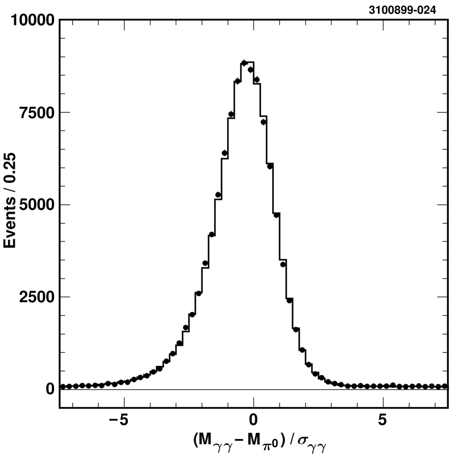
FIG. 1.: Normalized $M_{\gamma\gamma}$ distribution for $\pi^{0}$ candidate photon pairs in the data (points) and the generic $\tau$ Monte Carlo sample (line histogram), after all other cuts.

Of these, 94948 lie in the $\pi^{0}$ signal region, defined to be the interval $-3.0<S_{\gamma\gamma}<2.0$. The asymmetry of the distribution and the signal region definition arises because of the asymmetric energy response of the calorimeter. The low-side tail of the photon energy response curve is due primarily to rear and transverse leakage of high energy showers out of the CsI crystals whose energy depositions are summed in determining the energy of a given photon. We also make use of 2281 events lying in the side-band regions $-7.5<S_{\gamma\gamma}<-5.0$ and $3.0<S_{\gamma\gamma}<5.5$ to model backgrounds associated with spurious $\pi^{0}$ candidates. After these selections, we redetermine the photon energies and angles making use of the $\pi^{0}$ mass constraint, so as to improve the $\pi^{-}\pi^{0}$ invariant mass resolution.

The $M_{\pi^{-}\pi^{0}}$ spectrum is shown, after side-band subtraction, in Fig. 2.

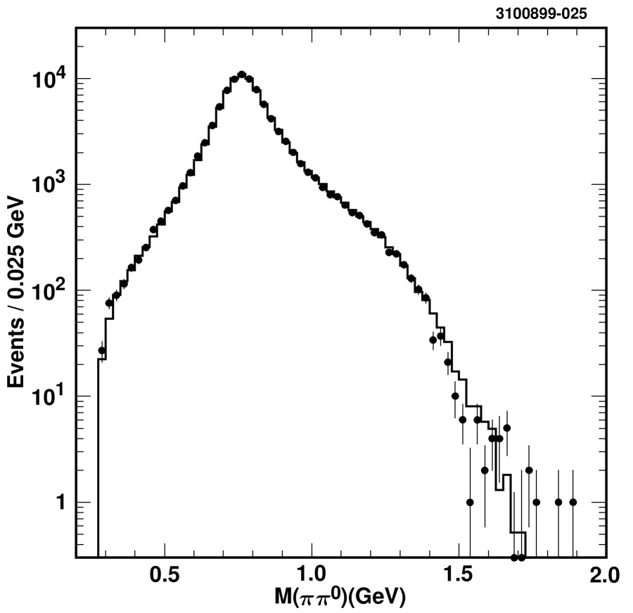
FIG. 2.: Raw $M_{\pi^{-}\pi^{0}}$ spectrum after $\pi^{0}$ side-band subtraction for candidate decays from the data (points) and the generic $\tau$ Monte Carlo sample (line histogram).

The agreement between data and MC spectra is more than an indication of the validity of the application of CVC. It also suggests that the event kinematics in the MC samples are sufficiently similar to those in the data that the selection criteria described above are not likely to have introduced significant biases. Additional support for this is the comparison between data and generic Monte Carlo samples of the $\pi^{-}$ momentum and $\pi^{0}$ energy distributions, shown in Figs. 3 and 4. Several events in Fig. 2 lie above the $\tau$ lepton mass. The small number of these events indicates that possible backgrounds at high mass, such as low-multiplicity $q\overline{q}$ events, are not significant.

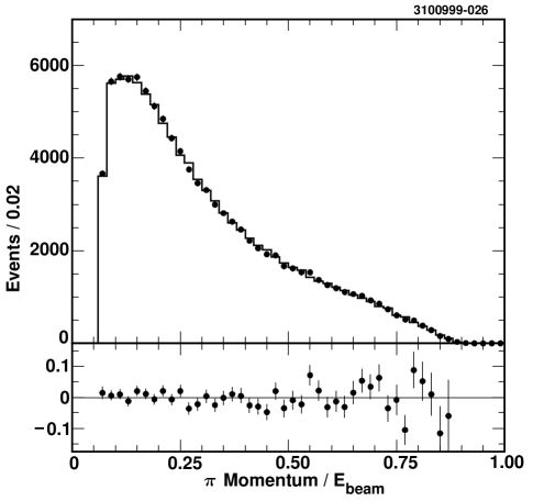
FIG. 3.: Distribution in the momentum of the $\pi^{-}$, divided by the beam energy, for candidate decays, from the data (points) and the generic $\tau$ Monte Carlo (line histogram) samples, after $\pi^{0}$ side-band subtraction. The bottom plot gives the deviations of the data spectrum from the Monte Carlo spectrum, normalized by the Monte Carlo spectrum.

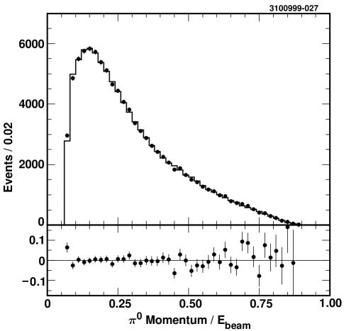
FIG. 4.: Distribution in the energy of the $\pi^{0}$, divided by the beam energy, for candidate decays, from the data (points) and the generic $\tau$ Monte Carlo (line histogram) samples, after $\pi^{0}$ side-band subtraction. The bottom plot gives the deviations of the data spectrum from the Monte Carlo spectrum, normalized by the Monte Carlo spectrum.

After $\pi^{0}$ side-band subtraction, backgrounds from non-signal $\tau$ decays are estimated to be $6.63\pm 0.20\,\%$ from the generic $\tau$ Monte Carlo sample. The dominant channels are $\tau^{-}\to\pi^{-}\pi^{0}\pi^{0}\nu_{\tau}$ ($4.01\pm 0.08\,\%$), $\tau^{-}\to K^{-}\pi^{0}\nu_{\tau}$ ($1.86\pm 0.16\,\%$) and $\tau^{-}\to h^{-}K^{0}_{L}\pi^{0}\nu_{\tau}$ ($0.59\pm 0.08\,\%$), where $h$ denotes $\pi$ or $K$ and the errors include branching fraction uncertainties as well as statistical errors.

IV CORRECTIONS TO THE DATA

One goal of this analysis is to analyze the $\pi^{-}\pi^{0}$ mass spectrum in the context of several models. However, we are not able to explore all possible models. In addition, it is desirable to compare our spectrum to data from other experiments in a model independent way, as well as to present it in a form that facilitates comparison with future data or models. These considerations motivate us to construct a histogram of the mass spectrum that has been corrected for (primarily) experimental effects. We then carry out simple $\chi^{2}$ fits to the corrected spectrum using the models of the $\pi^{-}\pi^{0}$ line shape described earlier.

Three experimental effects give rise to distortions in the $\pi^{-}\pi^{0}$ mass spectrum: (1) backgrounds; (2) smearing due to resolution and radiative effects; and (3) mass-dependence of the experimental acceptance. In this section, we describe the corrections, that we applied in the order listed to remove these distortions. These corrections rely on the Monte Carlo simulation of the physics and detector response.

A Binning of the $M_{\pi^{-}\pi^{0}}$ Spectrum

Before discussing the corrections mentioned above, we note that we have elected to bin the $M_{\pi^{-}\pi^{0}}$ spectrum in intervals of 25 MeV below 1 GeV, and 50 MeV above 1 GeV. This binning is chosen so as to be sensitive to rapidly varying regions of the spectrum while limiting the size of the bin migration correction and consequently the magnitude of correlations among nearby bins in the corrected spectrum. This is important for the stability and accuracy of the $\chi^{2}$ fit procedure, which is known to be biased when data points are strongly correlated [26]. The increase in mass resolution from approximately 6 MeV at low masses to 17 MeV at high masses motivates the large bin width above 1 GeV. The large bin width is also beneficial in the very high mass bins where low statistics could lead to non-Gaussian fluctuations.

B Corrections for Backgrounds

As noted earlier, the backgrounds entering the $\tau^{-}\to\pi^{-}\pi^{0}\nu_{\tau}$ sample are small. Side bands in the $M_{\gamma\gamma}$ distribution are used to model the fake-$\pi^{0}$ contribution. The remaining $6.6\%$ are modeled with the generic $\tau$-pair Monte Carlo sample. These subtractions are performed bin by bin in the mass spectrum. The Monte Carlo spectra for the signal and primary background modes are plotted in Fig. 5, after $\pi^{0}$ side-band subtraction.

FIG. 5.: Contributions to the reconstructed $M_{\pi^{-}\pi^{0}}$ spectrum from Monte Carlo simulation of signal and background $\tau$ decays. From bottom to top spectra for the following channels are plotted cumulatively: $\tau\to K_{L}h\pi^{0}\nu$ ($h$ denoting $\pi$ or $K$), $\tau\to\pi\pi^{0}\pi^{0}\nu$, $\tau\to K\pi^{0}\nu$ (backgrounds), and $\tau\to\pi\pi^{0}\nu$ (signal).

C Correction for Bin Migration

Detector resolution causes the $\pi^{-}\pi^{0}$ mass spectrum to become broader. The presence of radiation in the decay $\tau^{-}\to\pi^{-}\pi^{0}(\gamma)\nu_{\tau}$ is also important. The radiative photons tend to be low in energy, and are difficult to distinguish from photons from a possible second $\pi^{0}$ or from fragments of the hadronic shower from charged pions that interact in the calorimeter. Consequently, we can not identify them reliably, either for inclusion in the invariant mass calculation or as a basis for vetoing events. The net effect of ignoring decay radiation is to broaden and shift the mass spectrum.

We correct for these effects by performing an approximate unfolding procedure, based on a bin migration matrix determined from the $\tau^{-}\to\pi^{-}\pi^{0}\nu_{\tau}$ MC sample. This procedure is outlined in Appendix A. Since the experimental resolution on $M_{\pi\pi^{0}}$ is dominated by that on the $\pi^{0}$ energy, the agreement between data and MC shown in Fig. 1 gives us confidence in this aspect of the correction procedure. For the radiative effect, we rely on the PHOTOS-based simulation [22] employed by TAUOLA. The unfolded spectrum is shown as the dashed histogram in Fig. 6, with the uncorrected spectrum overlaid.

FIG. 6.: Effect of bin migration correction: $M_{\pi^{-}\pi^{0}}$ spectrum prior to (solid histogram with points), and after (dashed histogram) unfolding of resolution and radiative distortions.

D Correction for Acceptance

Finally we correct for mass dependence of the acceptance, plotted in Fig. 7. Again, this is determined from the MC simulation. The main effects causing this dependence are associated with the kinematics of the decay and the cuts imposed in the event selection, both of which are well understood.

FIG. 7.: Acceptance as a function of generated $\pi^{-}\pi^{0}(\gamma)$ mass, as determined from the full $\tau^{-}\to\pi^{-}\pi^{0}\nu_{\tau}$ Monte Carlo sample.

E The Corrected Mass Spectrum

The corrected mass spectrum is given in tabular form in Appendix B, along with elements of the covariance matrix characterizing the statistical errors and the correlations among entries introduced by the bin migration correction procedure. The spectrum is also made available electronically [23].

V RESULTS OF FITS FOR RESONANCE PARAMETERS

A Fitting Procedure

We perform $\chi^{2}$ fits to the fully-corrected $\pi^{-}\pi^{0}$ mass spectrum to extract resonance parameters and couplings. The $\chi^{2}$ minimization and parameter error determination is carried out using the MINUIT program [24]. Because of poor statistics and/or uncertainties associated with the background estimation and acceptance correction, only data in the range 0.5 to 1.5 GeV are included in the fits. Also, as a result of the unfolding procedure, off-diagonal terms of the covariance matrix are non-zero, and the corresponding terms must be included in the calculation of the $\chi^{2}$ [25]. The off-diagonal elements of the covariance matrix are not reflected in the error bars shown in the figures in this section.

Since the functional forms used to fit the data are nonlinear functions of many parameters, several iterations of minimization are performed before convergence is reached. We also integrate the fit function within each bin when computing the $\chi^{2}$. We have tested this procedure using high-statistics generator-level Monte Carlo samples to ensure the reproducibility and accuracy in the determination of fit parameters and their errors.

B Fit to the K&S Model

In this section, we report in detail the results from the simplest fit, done using the K&S model with no $\rho^{\prime\prime}$ contribution. Although this model is normalized according to the $F_{\pi}(0)=1$ constraint, we introduce an additional parameter multiplying the K&S function (Eq. 5), which is allowed to float in the fit. We have elected to do this for several reasons. First, we do not expect this or any other model of the line shape of a broad resonance to hold arbitrarily far from its peak. If the model does not hold at very low values of $M_{\pi^{-}\pi^{0}}$ then enforcing the $F_{\pi}(0)=1$ condition can bias the resonance parameters. Second, the focus of this analysis has been on the shape of the mass spectrum: for example, tight cuts have been applied to maintain high purity. The normalization of this spectrum (see Sec. VII B) depends on external measurements which have experimental uncertainties, as well as on theoretical factors which also have uncertainties. Given these considerations, the value of strictly enforcing the normalization condition is questionable.

The fully corrected $M_{\pi\pi^{0}}$ spectrum with the fit function superimposed is displayed in Fig. 8.

FIG. 8.: Fully corrected $M_{\pi^{-}\pi^{0}}$ distribution in $\tau^{-}\to\pi^{-}\pi^{0}\nu_{\tau}$ events (points). The solid curve overlaid represents the results of the fit to the K&S model. The dashed curve is obtained using the $\rho(770)$ parameters obtained from this fit, but with the $\rho^{\prime}$ contribution turned off (i.e., $\beta$ set to zero).

The $\chi^{2}$ for this fit is 27.0 for 24 degrees of freedom. We obtain

$$M_{\rho} = 774.9\pm 0.5\pm 0.9\;{\rm MeV},$$

$$\Gamma_{\rho} = 149.0\pm 1.1\pm 0.7\;{\rm MeV},$$

$$\beta = -0.108\pm 0.007\pm 0.005,$$

$$M_{\rho^{\prime}} = 1364\pm 7\pm 8\;{\rm MeV},$$

$$\Gamma_{\rho^{\prime}} = 400\pm 26\pm 23\;{\rm MeV},$$

where the first error is statistical and the second is due to systematic uncertainties, described in Sec. VI. When interpreted in terms of the pion form factor, the normalization gives $|F_{\pi}(0)|^{2}=1.16\pm 0.02$, where the error is statistical only. Performing the same fit, but with the $F_{\pi}(0)=1$ normalization condition imposed, yields a $\chi^{2}$ of 62.1 for 25 degrees of freedom and significantly different values for the other fit parameters (i.e., $M_{\rho}=772.3\,\mbox{\rm MeV},\;\Gamma_{\rho}=144.6\,\mbox{\rm MeV}$).

The fit parameters are correlated, with the correlation matrix:

$$\left(\begin{array}[]{rrrrrr}1.00&&&&&\\ 0.64&1.00&&&&\\ 0.75&0.51&1.00&&&\\ 0.89&0.68&0.43&1.00&&\\ 0.21&0.22&0.21&0.16&1.00&\\ -0.52&-0.38&-0.08&-0.74&\phantom{-}0.33&\phantom{-}1.00\end{array}\right),$$ (14)

where the parameters are normalization, $M_{\rho}$, $\Gamma_{\rho}$, $\beta$, $M_{\rho^{\prime}}$, and $\Gamma_{\rho^{\prime}}$, respectively.

C Fits to Other Models

The results from fits of the corrected $M_{\pi^{-}\pi^{0}}$ spectrum to various models are given in Table I.

TABLE I.: Results from fits to the corrected $M_{\pi^{-}\pi^{0}}$ spectrum over the range 0.5–1.5 GeV, for several models. The errors shown are statistical only. K&S refers to the model of Kühn and Santamaria [13] while G&S refers to the model of Gounaris and Sakurai [11]. See text for descriptions of these models and their variants.

Fit Parameter	Model
	K&S	K&S w/$\rho^{\prime\prime}$	K&S w/barrier	G&S	G&S w/$\rho^{\prime\prime}$
$M_{\rho}$ (MeV)	$774.9\pm 0.5$	$774.6\pm 0.6$	$769.7\pm 0.7$	$775.3\pm 0.5$	$775.1\pm 0.6$
$\Gamma_{\rho}$ (MeV)	$149.0\pm 1.1$	$149.0\pm 1.2$	$145.8\pm 1.3$	$150.5\pm 1.1$	$150.4\pm 1.2$
$\beta$	$-0.108\pm 0.007$	$-0.167\pm 0.008$	$-0.160\pm 0.008$	$-0.084\pm 0.006$	$-0.121\pm 0.009$
$M_{\rho^{\prime}}$ (MeV)	$1364\pm 7$	$1408\pm 12$	$1321\pm 9$	$1365\pm 7$	$1406\pm 13$
$\Gamma_{\rho^{\prime}}$ (MeV)	$400\pm 26$	$502\pm 32$	$397\pm 17$	$356\pm 26$	$455\pm 34$
$R_{\rho}$ (GeV-1)	—	—	$1.9\pm 0.3$	—	—
$R_{\rho^{\prime}}$ (GeV-1)	—	—	$5.0\pm 2.2$	—	—
$\gamma$	$\equiv 0$	$0.050\pm 0.010$	$\equiv 0$	$\equiv 0$	$0.032\pm 0.009$
$|F_{\pi}(0)|^{2}$	$1.16\pm 0.02$	$1.14\pm 0.02$	$0.39\pm 0.01$	$1.04\pm 0.02$	$1.03\pm 0.02$
$\chi^{2}$/dof	27.0/24	23.2/23	22.9/22	26.8/24	22.9/23

Several of these fits are illustrated in Fig. 9.

FIG. 9.: Alternate fits to the fully corrected $M_{\pi^{-}\pi^{0}}$ distribution in $\tau^{-}\to\pi^{-}\pi^{0}\nu_{\tau}$ events (points). The solid curve overlaid represents the results of the fit to the K&S model with $\rho^{\prime\prime}$ contribution included. The dashed curve represents the fit to the G&S model, also with the $\rho^{\prime\prime}$. The dotted curve is the fit to the K&S model, including the Blatt-Weisskopf barrier factor but no $\rho^{\prime\prime}$. The inset shows the low mass region where the differences between the models are most significant. Here we plot $|F_{\pi}|^{2}$ (see Sec. VII B), eliminating the purely kinematic factors which cause rapid variation in $M_{\pi^{-}\pi^{0}}$ in this region.

For fits including a $\rho^{\prime\prime}$ contribution, we fix its parameters to world average values [27] ($M_{\rho^{\prime\prime}}=1.700\,\mbox{\rm GeV},\;\Gamma_{\rho^{\prime\prime}}=0.235\,\mbox{\rm GeV}$), but allow the relative coupling constant $\gamma$ to float.

The G&S fits behave similarly to the K&S fits, as suggested by the $\chi^{2}$ values in Table I, and by the nearly overlapping solid and dashed curves in Fig. 9. In the figure, the deviation between the K&S and G&S curves is only visible at very low and very high values of $M_{\pi^{-}\pi^{0}}$. The deviation at low values is reflected by the difference in the inferred extrapolations of $|F_{\pi}|^{2}$ to $q^{2}=0$, where the G&S model gives results more consistent with the expectation $F_{\pi}(0)=1$.

The presence of the $\rho^{\prime\prime}$ in $e^{+}e^{-}\to\pi^{+}\pi^{-}$ is evident from the cross section measurements of DM2 [28] near and above $M_{\tau}$. For $\tau$ lepton decay, the $\rho^{\prime\prime}$ pole mass is near the endpoint of the $M_{\pi^{-}\pi^{0}}$ spectrum, thus making it difficult to observe. However, as with the $\rho^{\prime}$, its influence can be observed as an interference effect. While we obtain good fits without the $\rho^{\prime\prime}$ meson, the $\chi^{2}$ values for both K&S and G&S models are significantly improved when such a contribution is introduced. It can be seen in Fig. 9 that the $\rho^{\prime\prime}$ fits also agree better with the data points in the 1.5–1.6 GeV region which were excluded from the fits.

The relative phases of $\rho$, $\rho^{\prime}$ and $\rho^{\prime\prime}$ which we have obtained as $(+\,-\,+)$ are consistent with expectations from some models [16, 29]. We also find that including the $\rho^{\prime\prime}$ has a significant impact on our measurement of the $\rho^{\prime}$ parameters. In particular, values for the $\rho^{\prime}$ mass are closer to those based on other decay modes [27, 30] when the $\rho^{\prime\prime}$ is included.

We have also modified the energy dependence of the $\rho$ and $\rho^{\prime}$ widths by including the Blatt-Weisskopf factor (see Eq. 9). The results for the nominal K&S fit function (with no $\rho^{\prime\prime}$ contribution) modified in this way are given in Table I and shown as the dotted curve in Fig. 9. Values obtained for the $\rho$ and $\rho^{\prime}$ range parameters $R_{\rho}$ and $R_{\rho^{\prime}}$ are consistent with expectations. This fit yields a smaller $\chi^{2}$ per degree of freedom than other fits that also do not include the $\rho(1700)$. However, this function as implemented does not yield a normalization consistent with $F_{\pi}(0)=1$.

VI SYSTEMATIC ERRORS

Systematic errors are listed in Table II. These have been determined for the nominal K&S fit, however they are representative of those associated with G&S type fits as well. We have not included uncertainties associated with model dependence in our systematic error assessment. We discuss the most significant sources of error below.

TABLE II.: Systematic errors, in MeV except those for $\beta$, which is dimensionless.

Source	$M_{\rho}$	$\Gamma_{\!\rho}$	$\beta$	$M_{\rho^{\prime}}$	$\Gamma_{\!\rho^{\prime}}$
Backgrounds	0.1	0.4	0.002	1	5
Bin Migration	0.3	0.5	0.001	5	16
Momentum Scale	0.2	0.1	$<0.001$	1	1
Energy Scale	0.8	0.2	$0.002$	2	6
Acceptance	0.2	0.2	0.004	5	15
Fit Procedure	0.1	0.2	$<0.001$	1	1
Total Syst.	0.9	0.7	0.005	8	23
Stat. Error	0.5	1.1	0.007	7	26

A Background Subtraction

We rescale the individual background components by amounts consistent with uncertainties in branching fractions and detection efficiency. Typically, this is $\pm(5\mbox{\rm--}10)\%$ of the nominal. The largest change in fit parameters comes about by varying the $\tau^{-}\to K^{-}\pi^{0}\nu_{\tau}$ contribution in this way.

B Bin Migration Correction

The resolution on $M_{\pi^{-}\pi^{0}}$ is dominated by the photon energy measurement. The excellent agreement between data and MC seen in the $\pi^{0}$ mass spectra in Figure 1 gives us confidence that this resolution function is adequately simulated. That the MC correctly models radiative effects is tested by comparing characteristics of photon-like showers accompanying the $\pi^{-}\pi^{0}$ system with those in the data.

The method applied to unfold these effects relies on the approximate similarity between the $M_{\pi^{-}\pi^{0}}$ line shape used as input to the MC and the true one (see Appendix A). We have estimated the bias resulting from the inaccuracy of this approximation, and find it to be small. Considering this bias and possible errors in the modeling of the effects themselves, we conservatively arrive at the uncertainties shown in Table II. For reference, failure to correct for bin migration results in values for $M_{\rho}$ and $\Gamma_{\!\rho}$ which are 2.6 MeV lower and 4.6 MeV higher, respectively. Thus we believe we understand this correction to $\sim 10\%$ of itself.

C Energy and Momentum Scales

Although the $\pi^{0}$ mass resolution function is well modeled, even a small error in the absolute energy calibration of the calorimeter can have an effect on $M_{\rho}$ without grossly disturbing the agreement in Figure 1. Based on studies of photons from various processes, we believe this calibration to be good to better than 0.3% [31]. Scaling the photon energies in the data by a factor of $1\pm 0.003$ and fitting the $M_{\pi^{-}\pi^{0}}$ spectra thus obtained results in the uncertainties shown in Table II.

The same procedure is used to assess the systematic error due to the absolute momentum scale uncertainty. Studies of $D$ meson decays and $e^{+}e^{-}\to\mu^{+}\mu^{-}$ events have demonstrated that the momentum scale uncertainty is below $0.05\%$ [32].

D Other Sources of Error

To estimate errors associated with the mass dependence of the detection efficiency, we modified the shape of the acceptance correction distribution (Fig. 7) by amounts suggested by the variation of selection criteria. We also performed the full analysis after varying cuts on $S_{\gamma\gamma}$, minimum photon energy, and the $\pi^{0}\to\gamma\gamma$ decay angle. Uncertainties associated with the fitting procedure were evaluated by performing fits to generator-level Monte Carlo spectra (no detector effects simulated). We also fit the uncorrected data and MC spectra, using the observed shifts in fit parameters for the MC sample to correct the parameters obtained from the data sample. This procedure yielded results that were in agreement with our nominal procedure. As a final cross-check, we split the data sample according to the tag decay. The results obtained for the three tags were in agreement with each other.

VII COMPARISON WITH DATA FROM OTHER EXPERIMENTS

A Comparison with Fits by Other Experiments

The results from our fits can be compared with similar fits by ALEPH [6] to their data, as well as with fits by other authors [13, 14, 18] to various compilations of $e^{+}e^{-}\to\pi^{+}\pi^{-}$ data. For illustration purposes, some representative comparisons are given in Table III.

TABLE III.: Comparison of results of fits using the K&S and G&S models ($\rho^{\prime\prime}$ included with $M_{\rho^{\prime\prime}},\ \Gamma_{\rho^{\prime\prime}}=1700,\ 235$ MeV) to (a) CLEO $\tau$ data, (b) ALEPH $\tau$ data [6] and (c) $e^{+}e^{-}\to\pi^{+}\pi^{-}$ data (denoted ‘K&S Fit’, from fits in Ref. [13]). Units are MeV for all fit parameters, except $\beta$, $\gamma$ and $|F_{\pi}(0)|^{2}$ which are dimensionless. Shown in parentheses are the experimental uncertainties (statistical plus systematic). The parameter associated with $\rho$-$\omega$ interference in the $e^{+}e^{-}$ data is not shown.

Parameter	K&S Model			G&S Model
	CLEO	ALEPH	K&S Fit	CLEO	ALEPH	K&S Fit
$M_{\rho}$	$774.6\,(1.1)$	$774.9\,(0.9)$	773	$775.1\,(1.1)$	$776.4\,(0.9)$	776
$\Gamma_{\rho}$	$149.0\,(1.4)$	$144.2\,(1.5)$	144	$150.4\,(1.4)$	$150.5\,(1.6)$	151
$\beta$	$-0.167\,(10)$	$-0.094\,(7)$	$-0.103$	$-0.121\,(10)$	$-0.077\,(8)$	$-0.052$
$M_{\rho^{\prime}}$	$1408\,(14)$	$1363\,(15)$	1320	$1406\,(15)$	$1400\,(16)$	1330
$\Gamma_{\rho^{\prime}}$	$502\,(39)$	$\equiv 310$	$390$	$455\,(41)$	$\equiv 310$	$270$
$\gamma$	$0.050\,(10)$	$-0.015\,(8)$	$-0.037$	$0.032\,(9)$	$0.001\,(9)$	$-0.031$
$|F_{\pi}(0)|^{2}$	$1.14\,(2)$	$\equiv 1$	$\equiv 1$	$1.03\,(2)$	$\equiv 1$	$\equiv 1$
$\chi^{2}$/dof	23.2/23	81/65	136/132	22.9/23	54/65	151/132

For the $e^{+}e^{-}$ data we give the results of the fits carried out by Kühn and Santamaria [13] to data below $\sqrt{s}\sim 1.6$ GeV. These authors did not quote uncertainties on the parameters they obtained. However, based on similar fits performed by Barkov et al. [18] and by us, we believe these uncertainties to be similar in magnitude to those from the $\tau$ decay data fits. For example, averaging over models, Ref. [18] obtains $M_{\rho}=775.9\pm 0.8\pm 0.8$ GeV, $\Gamma_{\rho}=150.5\pm 1.6\pm 2.5$ GeV, where the first error represents that due to statistics plus systematics, and the second error gives the uncertainty due to model dependence.

The comparisons given in Table III are not meant to be rigorous. Due to the different assumptions made by different authors, a systematic comparison is not possible. For example, the choice of whether to enforce the $F_{\pi}(0)=1$ condition for the K&S model has a strong impact on the fit parameters and the goodness of fit for the $\tau$ data (see Sec. V B). In the G&S model this choice is less crucial since the values of $|F_{\pi}(0)|^{2}$ obtained when it is allowed to float are closer to unity than they are in the K&S model. In addition, the fits to the $e^{+}e^{-}$ data shown do not include the high-$\sqrt{s}$ data from DM2 [28]. With this data included, fits we have carried out yield results that are considerably different from those with this data excluded. The applicability of any given model across the full range of $\sqrt{s}$ accessible to experiments has not been demonstrated.

Finally, small differences between charged and neutral $\rho$ meson parameters are expected, due to manifestations of isospin violation such as the $\pi^{-}/\pi^{0}$ mass difference. Refs. [4] and [6] include discussions of this issue. Additional comments are given in Appendix C.

With these caveats, Table III demonstrates general agreement between CLEO and ALEPH data, and between the $\tau$ and $e^{+}e^{-}$ data, supporting the applicability of CVC. In particular, the Gounaris-Sakurai fits show very good agreement between CLEO and ALEPH data. Within the K&S model, the smaller values of $\Gamma_{\rho}$ obtained for the ALEPH and $e^{+}e^{-}$ data are likely a consequence of the $F_{\pi}(0)=1$ constraint, as similar values are also obtained when this constraint is imposed for the CLEO data (see Sec. V B).

B Model Independent Comparisons

1 Comparison of CLEO and ALEPH data

It is also useful to compare data from different experiments in a model-independent way. The ALEPH Collaboration has published their corrected $M^{2}_{\pi^{-}\pi^{0}}$ spectrum [6], which may be compared directly with the corresponding CLEO spectrum. Given the differences in binning, a visually useful comparison is obtained by determining the bin-by-bin deviations of the two data sets from the prediction of a given model. For the prediction we use the results from the fit of the CLEO data to the G&S model, including $\rho^{\prime\prime}$. In Fig. 10, we plot the deviations of the CLEO and ALEPH data from this model as a function of $M_{\pi^{-}\pi^{0}}$.

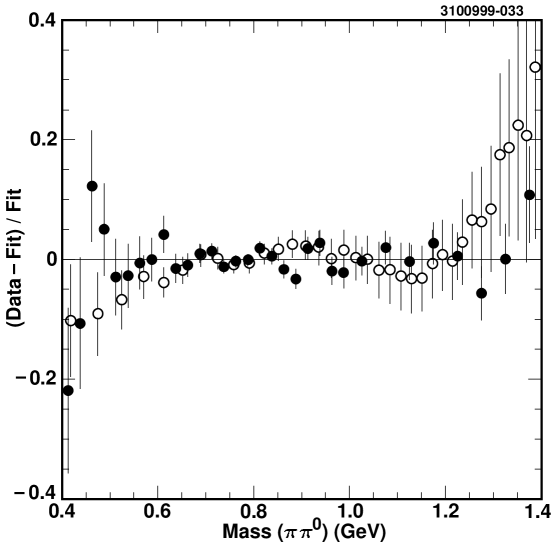
FIG. 10.: Difference in $\overline{v}(M_{\pi^{-}\pi^{0}})$ of CLEO (filled circles) and ALEPH (open circles) data from the fit of the CLEO $\tau^{-}\to\pi^{-}\pi^{0}\nu_{\tau}$ data to the Gounaris-Sakurai model, with $\rho^{\prime\prime}$ included, divided by the fit value.

The clustering of the CLEO points around zero is expected given the goodness of the fit. The ALEPH points also cluster around zero, although systematic deviations may be present at low and high masses. The significant correlations among the ALEPH points make this difficult to establish from the figure. Independent of possible deviations from the model, however, the CLEO and ALEPH points show agreement over the entire spectrum.

2 Comparison of CLEO and $e^{+}e^{-}$ data

Direct comparison, independent of model, of $\tau$ and $e^{+}e^{-}$ data can also be made as a further test of CVC. To do this we represent the fully corrected CLEO $\pi^{-}\pi^{0}$ mass spectrum in terms of $|F_{\pi}|^{2}$ which can be compared with the $e^{+}e^{-}$ data directly. Using the leptonic $\tau$ decay width $\Gamma_{e}=G_{F}^{2}M_{\tau}^{5}S^{e}_{EW}/192\pi^{3}$ and the ratio of $\tau$ decay branching fractions to $\pi^{-}\pi^{0}\nu_{\tau}$ ($B_{\pi\pi^{0}}$) and $e^{-}\overline{\nu}_{e}\nu_{\tau}$ ($B_{e}$) for normalization, we derive the spectral function averaged over each mass bin from Eq. 1:

$$\overline{v}^{\pi\pi}(M_{i})=\frac{B_{\pi\pi^{0}}}{B_{e}}\,\frac{M_{\tau}^{8}}{12\pi\,|V_{ud}|^{2}}\,\frac{S^{e}_{EW}}{S^{\pi\pi}_{EW}}\,\frac{1}{M_{i}\,(M_{\tau}^{2}-M_{i}^{2})^{2}\,(M_{\tau}^{2}+2M_{i}^{2})}\,\frac{1}{N}\,\frac{N_{i}}{\Delta M_{i}},$$ (15)

where $M_{i}$ is the central value of $M_{\pi^{-}\pi^{0}}$ for the $i^{th}$ bin, and the quantity $1/N\,N_{i}/\Delta M_{i}$ is the number of entries ($N_{i}$) in the $i^{th}$ bin of the corrected measured $\pi^{-}\pi^{0}$ mass spectrum, divided by the total number of entries ($N$) and the bin width ($\Delta M_{i}$). We use world average values [27] for the branching fractions, $B_{\pi\pi^{0}}=(25.32\pm 0.15)\,\%$ and $B_{e}=(17.81\pm 0.07)\,\%$, for the $\tau$ lepton mass $M_{\tau}=1777.05^{+0.29}_{-0.26}$ MeV, and for the CKM element $|V_{ud}|=0.9752\pm 0.08$. $S^{e}_{EW}$ represents the radiative corrections to leptonic $\tau$ decay, evaluated to be 0.996 (see Ref. [7]). The overall radiative correction factor $S_{EW}=S^{\pi\pi}_{EW}/S^{e}_{EW}$ is estimated to be 1.0194 [9], based mainly on the logarithmic terms associated with short-distance diagrams involving loops containing bosons, which differ for leptonic and hadronic final states. Non-logarithmic terms have not yet been computed for the $\pi\pi$ final state, but are expected to be small.

$|F_{\pi}(M)|^{2}$ is computed from $\overline{v}(M)$ using Eq. 4. A small ($<1\%$) correction is made to represent each point as a measurement at the central value of its mass bin, rather than as an average over the bin. This is done by employing the results from the fits described earlier to estimate the effect of the line shape variation across each of the histogram bins. Although this correction depends on the model used, this model-dependence is negligible relative to experimental errors. The factors appearing in Eqs. 4 and 15 are also used to recast the normalization parameters determined in the fits described in Sec. V in terms of $|F_{\pi}(0)|^{2}$, as shown in Table I.

In Figure 11, the values of $|F_{\pi}|^{2}$ derived from the corrected CLEO $M_{\pi^{-}\pi^{0}}$ spectrum are plotted along with the with $e^{+}e^{-}\to\pi^{+}\pi^{-}$ data from CMD [18], CMD-2 [33], DM1 [34], DM2 [28], OLYA [18], NA7 [35], as well as Adone [36, 37, 38] experiments and other VEPP [18, 39] experiments.

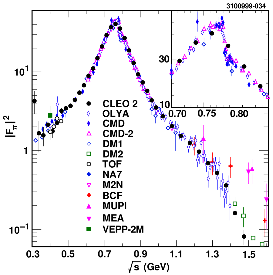
FIG. 11.: Comparison of $|F_{\pi}|^{2}$ as determined from CLEO-II $\tau^{-}\to\pi^{-}\pi^{0}\nu_{\tau}$ data (filled circles), with that obtained from $e^{+}e^{-}\to\pi^{+}\pi^{-}$ cross sections (other symbols) from CMD, CMD-2, DM1, DM2, OLYA, and NA7, as well as Adone and other VEPP experiments. The inset is a blow-up of the region near the $\rho$ peak, where $\rho$-$\omega$ interference is evident in the $e^{+}e^{-}$ data.

The $\tau$ data follow the $e^{+}e^{-}$ data shape well, except in the region where $\rho$-$\omega$ interference affects the $e^{+}e^{-}$ data. However, the $\tau$ data tend to lie above the $e^{+}e^{-}$ data throughout most of the range in $\sqrt{s}$. This is illustrated in Fig. 12, where we plot the fractional difference between measured values of $|F_{\pi}(s)|^{2}$ from the $e^{+}e^{-}$ data and the prediction from the G&S fit (including $\rho^{\prime\prime}$) to the CLEO $\tau$ data. To obtain this prediction, we modified the G&S fit function for use with $e^{+}e^{-}$ data. We allowed the normalization and a parameter associated with $\rho$-$\omega$ interference to float to determine the latter, and then readjusted the normalization to give that shown in Table I.

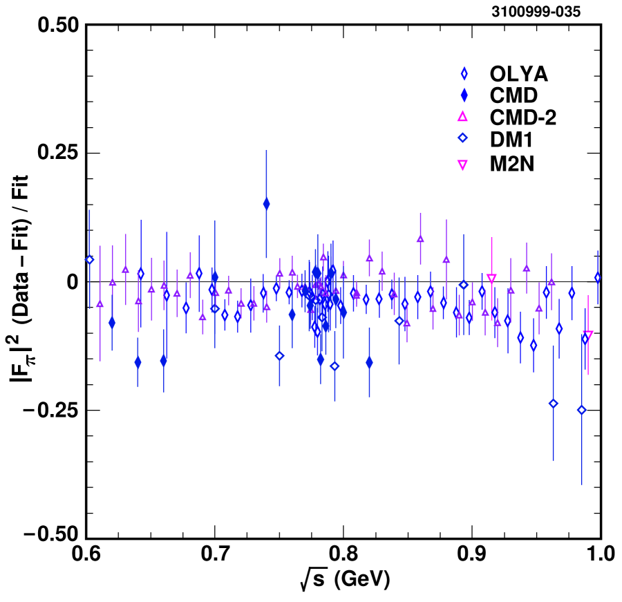
FIG. 12.: Difference between $|F_{\pi}|^{2}$ as determined from $e^{+}e^{-}\to\pi^{+}\pi^{-}$ data and that inferred from fit of the CLEO $\tau^{-}\to\pi^{-}\pi^{0}\nu_{\tau}$ data to the Gounaris-Sakurai model, with $\rho^{\prime\prime}$ included, divided by the fit value. The different symbols represent the data points from the $e^{+}e^{-}$ experiments operating in the $\rho$ peak region.

The deviation from zero in Fig. 12 is consistent with the deviation from unity of the value of $|F_{\pi}(0)|^{2}=1.03$ inferred from the fit to the CLEO $\tau$ data. (Fitting the $e^{+}e^{-}$ data with the normalization floating yields values of $|F_{\pi}(0)|^{2}\sim 1.00$.) It is also consistent with the observation made by Eidelman and Ivanchenko [40] that the measured $\tau^{-}\to\pi^{-}\pi^{0}\nu_{\tau}$ branching fraction is larger than that expected from application of CVC to the $e^{+}e^{-}\to\pi^{+}\pi^{-}$ data by $3.2\pm 1.4\,\%$. The consistency of these three indications of CVC violation is not accidental since they all involve (1) application of CVC to largely the same $e^{+}e^{-}$ data, as well as the use of (2) the world average value for the $\tau$ decay branching fractions [27] and (3) the same electroweak radiative correction factor [7, 9] to normalize the $\tau$ decay spectral function, as described above. Known sources of error in the first two of these components have been included in the $\pm 1.4\%$ error above. Recent estimates suggest that the uncertainty associated with additional radiative correction factors not yet computed could be as large as $\pm 0.4\%$ (see Refs. [4, 41]). Deviations associated with isospin-violating effects are expected to be small, but carry an uncertainty not reflected above.

VIII IMPLICATIONS FOR THE MUON ANOMALOUS MAGNETIC MOMENT

A Introduction and Motivation

The muon magnetic moment anomaly $a_{\mu}=(g_{\mu}-2)/2$ has an experimental value of $(11\,659\,230\pm 84)\times 10^{-10}$ [27, 42]. It receives significant contributions from uncalculable hadronic vacuum-polarization radiative corrections, estimated recently [43] to be $a_{\mu}^{had}=(692.4\pm 6.2)\times 10^{-10}$. The error on this contribution is the most significant source of uncertainty in the Standard Model prediction for $a_{\mu}$. Experiment E821 at Brookhaven National Laboratory, currently under way, is aiming at a precision of $\sim 4\times 10^{-10}$ in order to be sensitive to the weak interaction contribution at $15\times 10^{-10}$, as well as possible contributions from new physics. Improved knowledge of $a_{\mu}^{had}$ is important for interpreting experimental results on $a_{\mu}$. In this section, we discuss the implications of our data on $\tau^{-}\to\pi^{-}\pi^{0}\nu_{\tau}$ for the determination of $a_{\mu}^{had}$, following the first such treatment of $\tau$ decay data, by Alemany, Davier and Höcker [4] who used ALEPH data [6].

The value of $a_{\mu}^{had}$ is related to the $e^{+}e^{-}$ anihilation cross section to hadronic final states via the dispersion integral [44]

$$a_{\mu}^{had}=\frac{\alpha_{em}^{2}(0)}{\pi}\int_{4M_{\pi}^{2}}^{\infty}{\frac{ds}{s}\,v(s)\,K(s)},$$ (16)

where $v(s)$ denotes the inclusive hadronic spectral function, and $\alpha_{em}(0)$ is the fine structure constant. $K(s)$ is the QED kernel

$$K(s)=x^{2}\,\left(1-\frac{x^{2}}{2}\right)+(1+x)^{2}\,\left(1+\frac{1}{x^{2}}\right)\,\left(\ln{(1+x)}-x-\frac{x^{2}}{2}\right)+\left(\frac{1+x}{1-x}\right)\,x^{2}\,\ln{x}\,,$$ (17)

where $x=(1-\beta_{\mu})/(1+\beta_{\mu})$, with $\beta_{\mu}=(1-4M_{\mu}^{2}/s)^{1/2}$. Consequently, predictions for $a_{\mu}^{had}$ are based primarily on $e^{+}e^{-}$ data. By virtue of the form of $K(s)$ and the $1/s$ factor in the integrand above, measurements at low values of $\sqrt{s}$ where the $\pi^{+}\pi^{-}$ final state dominates are particularly significant.

B The Impact of $\tau$ Decay Data

The smallness of the present error on $a_{\mu}^{had}$ reflects the use of CVC and $\tau$ decay data from ALEPH [4] to improve the precision relative to that obtained based on $e^{+}e^{-}$ data alone. Specifically, the authors of Ref. [4] determine the $\pi^{+}\pi^{-}$ contribution over the interval $\sqrt{s}=0.320-2.125$ GeV to be

$$a_{\mu}^{\pi\pi}[0.320,\,2.125]=\left\{\begin{array}[]{cl}(495.86\pm 12.46)\times 10^{-10}&(e^{+}e^{-}\mbox{\rm\ data\ only})\\ (500.81\pm\phantom{1}6.03)\times 10^{-10}&(e^{+}e^{-}+\tau\mbox{\rm\ data})\end{array}\right.,$$ (18)

where the $e^{+}e^{-}$ data did not include the CMD-2 data [33] which were not available at that time. The combining of $e^{+}e^{-}$ and $\tau$ data was carried out by averaging data points from different experiments prior to integrating the data. An advantage of this procedure is that it properly weights the $\tau$ data more heavily in regions where it is more precise than the $e^{+}e^{-}$ data and vice-versa. Accordingly, the improvement in precision indicated in Eq. 18 is greater than that obtained by determining $a_{\mu}^{\pi\pi}$ separately for $\tau$ and $e^{+}e^{-}$ data and averaging the results.

In assessing the impact of the CLEO $\pi^{-}\pi^{0}$ spectral function on the value and precision of $a_{\mu}^{had}$, we perform the integration in Eq. 16 using our data alone. Although this procedure does not possess the benefit described above, future changes to the central values or errors of external factors such as $B_{\pi\pi^{0}}$ or $S_{EW}$ can be propagated easily. However, we note that a careful determination of $a_{\mu}^{had}$ would combine the data from different experiments in some fashion, for example along the lines of the approach described in Ref. [4].

Details of our determination of $a_{\mu}^{\pi\pi}$, including the method and corrections applied to account for isospin violating effects are presented in Appendix C. Here, we report our results for the same interval in $\sqrt{s}$ as in Eq. 18. We obtain

$$a_{\mu}^{\pi\pi}[0.320,\,2.125]=(513.1\pm 2.1\pm 3.0\pm 4.5)\times 10^{-10},$$ (19)

where the first error is due to statistics, the second error is due to experimental systematic uncertainies, and the third error reflects the uncertainties in externally determined quantities entering the calculation. These sources of error are discussed in Appendix C.

The deviation between the CLEO result above and the result from Ref. [4] given in Eq. 18 based on $e^{+}e^{-}\to\pi^{+}\pi^{-}$ data only is again indicative of disagreement in the normalizations, rather than in the shapes, of the $e^{+}e^{-}$ and $\tau$ spectral functions as discussed in the previous sections. While the magnitude of this deviation is not significant on the scale of the reported errors, both it and the errors are greater than the projected precision of the BNL E821 experiment. Continued efforts to precisely determine $a_{\mu}^{had}$ will be needed to help interpret the results of the Brookhaven experiment.

IX SUMMARY

From a sample of approximately 87000 decays (after subtraction of backgrounds) of the type $\tau^{-}\to\pi^{-}\pi^{0}\nu_{\tau}$, we have investigated structure in the $\pi^{-}\pi^{0}$ invariant mass spectrum. From fits to several models we have obtained parameters and relative couplings for the $\rho(770)$ and $\rho(1450)$ resonances. Within the Kühn and Santamaria model [13] with no $\rho(1700)$ contribution, the precisions on the $\rho(770)$ mass and width are 1.0 and 1.4 MeV, respectively. These precisions are comparable to those obtained by ALEPH [6] using the same $\tau$ decay mode, as well as those obtained from fits to low-energy $e^{+}e^{-}\to\pi^{+}\pi^{-}$ data [6, 13, 18].

We find that a successful description of our $M_{\pi^{-}\pi^{0}}$ spectrum requires interfering Breit-Wigner line shapes associated with $\rho(770)$ and $\rho(1450)$ resonances. Fits including additional contributions from the $\rho(1700)$ resonance are preferred, consistent with the observations of DM2 [28] in $e^{+}e^{-}\to\pi^{+}\pi^{-}$. Fits of comparable quality are also obtained without a $\rho^{\prime\prime}$ contribution when the mass-dependence of the $\rho$ and $\rho^{\prime}$ widths is modified to include Blatt-Weisskopf barrier factors. We find that Gounaris-Sakurai [11] type fits yield extrapolations to $q^{2}=0$ that are higher than but roughly consistent with $F_{\pi}(0)=1$. The Kühn-Santamaria [13] type fits lead to significantly higher values, such that imposing $F_{\pi}(0)=1$ can lead to biased values for $\rho$ and $\rho^{\prime}$ parameters.

Quantitatively, the central values for the precisely determined $\rho(770)$ parameters are difficult to compare with those from fits by others. This is due to severe model dependence and the strong influence of data far from the $\rho$ peak. Qualitatively, the shape of our $M_{\pi^{-}\pi^{0}}$ spectral function agrees well with that obtained by ALEPH [6]. It also agrees well with the $e^{+}e^{-}\to\pi^{+}\pi^{-}$ data, supporting the applicability of CVC. Using our spectral function, we have employed CVC to infer the significant component of the hadronic contribution to the muon $g-2$ factor associated with the $e^{+}e^{-}\to\pi^{+}\pi^{-}$ cross section, obtaining $a_{\mu}^{\pi\pi}[0.320,\,2.125]=(513.1\pm 5.8)\times 10^{-10}$.

However, we also observe indications of discrepancies between the overall normalization of $\tau$ and $e^{+}e^{-}$ data, as pointed out by Eidelman and Ivanchenko [40]. These appear in the model independent comparison of our spectrum with the $e^{+}e^{-}$ cross section measurements, as well as in the values for $|F_{\pi}(0)|^{2}$ inferred from fits to our spectrum which are larger than unity, and in our high value for $a_{\mu}^{\pi\pi}$. Though larger than the deviations expected due to known sources of isospin violation, these could also arise from experimental errors in the $\tau$ decay branching fraction measurements or the normalization of the $e^{+}e^{-}\to\pi^{+}\pi^{-}$ cross section measurements, or from theoretical uncertainties in the estimates of radiative corrections, or from all of these sources. At present the deviations are not significant on the scale of the reported errors. We hope that new data from Novosibirsk, BEPC, and the B-factory (PEP-II, KEK-B and CESR-III) storage rings will shed light on this issue in the near future.

A UNFOLDING OF RESOLUTION AND RADIATIVE EFFECTS

The unfolding procedure is used to correct for bin migration in the observed $M_{\pi\pi^{0}}$ spectrum due to resolution smearing and radiative effects. In this Appendix, we describe the procedure used in this analysis. In the discussion that follows, matrices are denoted in boldface, while non-bold symbols represent vectors with the contents of binned histograms.

The unfolding procedure makes use of the Monte Carlo to characterize the bin migration. One may construct a migration matrix $P$ which gives the probability that an event generated with a given $\pi^{-}\pi^{0}(\gamma)$ mass is reconstructed with a given $\pi^{-}\pi^{0}$ mass:

$$R^{\rm MC}=\mbox{\boldmath$P$}\,G^{\rm MC},$$ (A1)

where $G^{\rm MC}$ represents the generated $\pi^{-}\pi^{0}(\gamma)$ mass spectrum and $R^{\rm MC}$ represents the reconstructed one. It is possible to apply the inverse of $P$ to the spectrum observed in the data $R^{\rm data}$ to obtain an unfolded spectrum $U^{\rm data}$ that provides an estimate for the parent spectrum. However, such a procedure is not robust with respect to statistical fluctuations entering the determination of $P$, and can yield spectra with unphysically large point-by-point fluctuations.

The corrected ALEPH spectrum [6] was derived using a method based on singular value decomposition of the migration matrix [45] to mitigate this effect. Here, we use an iterative method that relies on the smallness of the bin migrations and the approximate similarity between the reconstructed spectra from the data ($R^{\rm data}$) and Monte Carlo ($R^{\rm MC}$) samples. We construct the matrix $P^{\prime}$, which gives the fraction of MC events with a given reconstructed $\pi^{-}\pi^{0}$ mass that were generated with a given $\pi^{-}\pi^{0}(\gamma)$ mass. With this matrix, $G^{\rm MC}=\mbox{\boldmath$P^{\prime}$}\,R^{\rm MC}$ is satisfied, but $P^{\prime}$ is not equal to $P^{-1}$. Successive application of $P^{\prime}$ to the observed data spectrum gives an estimate for the parent distribution, according to:

$$U^{\rm data}=\mbox{\boldmath$P^{\prime}$}\,R^{\rm data}+\sum_{k=1}^{\infty}{({\bf 1}-\mbox{\boldmath$P^{\prime}P$})^{k}\,\mbox{\boldmath$P^{\prime}$}\,(R^{\rm data}-R^{\rm MC})}.$$ (A2)

For small bin migration probabilities, all elements of the matrix $({\bf 1}-\mbox{\boldmath$P^{\prime}P$})$ are small: these elements are the ‘expansion parameters’ in the series above. A simpler form for Eq. A2 is obtained by recognizing that the quantity $({\bf 1}-\mbox{\boldmath$P^{\prime}P$})\mbox{\boldmath$P^{\prime}$}\,R^{\rm MC}$ is identically zero. As written, however, Eq. A2 illustrates that when the series is truncated, deviation from the results of the full expansion vanishes as $(R^{\rm data}-R^{\rm MC})\rightarrow 0$.

With the similarity between the observed data and MC spectra plotted in Fig. 2, we find it sufficient to ignore terms with $k>1$ in Eq. A2. The $k=1$ term has a noticeable effect on several of the fit parameters reported in Section V B. In particular, ignoring this term leads to a value for $\Gamma_{\rho}$ that is 0.5 MeV smaller than that from our nominal fit. Higher order terms have no significant impact on any of the parameters.

B THE CORRECTED $\pi^{-}\pi^{0}$ MASS SPECTRUM

In this appendix we present the fully corrected CLEO $M_{\pi\pi^{0}}$ spectrum in tabular form. The spectrum is given as a compilation of event yields for each mass bin in Table IV, normalized so that the sum of entries over all bins is unity. Also given are the square roots of the diagonal elements of the covariance matrix (statistical errors only).

TABLE IV.: The corrected CLEO $M_{\pi\pi^{0}}$ spectrum given in terms of event yield as a function of mass bin. The spectrum is normalized so that the number of entries sums to unity. The numbers in parentheses denote the square roots of the diagonal elements of the covariance matrix (statistical errors only). Note that the number of entries jumps at the 1.00–1.05 GeV bin, where the bin size is increased from 0.025 to 0.050 GeV.

Bin	Mass Range	Entries		Bin	Mass Range	Entries
No.	(GeV)	$(10^{-4})$		No.	(GeV)	$(10^{-4})$
1	0.275–0.300	$1.5\;(1.4)$
2	0.300–0.325	$8.0\;(2.5)$
3	0.325–0.350	$6.0\;(2.6)$
4	0.350–0.375	$8.5\;(2.3)$		24	0.850–0.875	$446.7\;(6.6)$
5	0.375–0.400	$15.6\;(2.6)$		25	0.875–0.900	$326.2\;(5.5)$
6	0.400–0.425	$16.2\;(2.9)$		26	0.900–0.925	$262.1\;(4.9)$
7	0.425–0.450	$24.9\;(3.1)$		27	0.925–0.950	$207.3\;(4.3)$
8	0.450–0.475	$41.4\;(3.4)$		28	0.950–0.975	$158.8\;(3.7)$
9	0.475–0.500	$50.6\;(3.7)$		29	0.975–1.000	$129.6\;(3.4)$
10	0.500–0.525	$60.9\;(4.0)$		30	1.000–1.050	$202.8\;(4.8)$
11	0.525–0.550	$79.8\;(4.4)$		31	1.050–1.100	$151.0\;(4.1)$
12	0.550–0.575	$107.4\;(4.7)$		32	1.100–1.150	$111.0\;(3.4)$
13	0.575–0.600	$144.3\;(5.2)$		33	1.150–1.200	$87.0\;(3.0)$
14	0.600–0.625	$204.5\;(5.9)$		34	1.200–1.250	$63.9\;(2.5)$
15	0.625–0.650	$269.1\;(6.5)$		35	1.250–1.300	$42.7\;(2.0)$
16	0.650–0.675	$385.8\;(7.5)$		36	1.300–1.350	$29.2\;(1.7)$
17	0.675–0.700	$571.5\;(8.7)$		37	1.350–1.400	$18.1\;(1.3)$
18	0.700–0.725	$826.8\;(10.1)$		38	1.400–1.450	$6.98\;(0.84)$
19	0.725–0.750	$1078.4\;(11.3)$		39	1.450–1.500	$2.91\;(0.59)$
20	0.750–0.775	$1228.1\;(11.8)$		40	1.500–1.550	$0.71\;(0.32)$
21	0.775–0.800	$1114.7\;(11.0)$		41	1.550–1.600	$0.59\;(0.25)$
22	0.800–0.825	$878.1\;(9.6)$		42	1.600–1.650	$0.68\;(0.26)$
23	0.825–0.850	$629.3\;(7.9)$		43	1.650–1.700	$0.28\;(0.21)$

The statistical errors given in Table IV do not reflect the correlations between data points that were introduced by the bin migration correction. Although the correlations are not large, proper treatment of these data necessitates use of the covariance matrix. The full covariance matrix $V$ is a $43\times 43$ symmetric matrix. In Table V, we present the correlation coefficients $\rho_{ij}=V_{ij}/(V_{ii}V_{jj})^{1/2}$ for bins $i$ and $j$, $i>j$, for $i,\,j$ where $\rho_{ij}>0.0015$. The coefficients shown are the statistical correlations only. Both the corrected spectrum as given in Table IV and the full covariance matrix are available electronically [23].

TABLE V.: Correlation coefficients $\rho_{ij}$ for contents of bins $i$ and $j$ (see Table IV) of the fully corrected CLEO $M_{\pi\pi^{0}}$ spectrum, for $i>j$. Coefficients with values less than 0.0015 are not shown. These coefficients reflect statistical correlations only.

$i$	$j$	$\rho_{ij}$		$i$	$j$	$\rho_{ij}$		$i$	$j$	$\rho_{ij}$		$i$	$j$	$\rho_{ij}$		$i$	$j$	$\rho_{ij}$		$i$	$j$	$\rho_{ij}$
2	1	$-.002$		10	8	$-.057$		16	14	$-.084$		21	19	$-.116$		28	27	$.299$		38	35	$-.011$
3	1	$-.031$		10	9	$.085$		16	15	$.183$		21	20	$.205$		29	25	$-.006$		38	36	$-.074$
3	2	$.042$		11	6	$-.002$		17	3	$.002$		22	18	$-.003$		29	26	$-.046$		38	37	$.114$
4	1	$.003$		11	8	$-.013$		17	11	$-.002$		22	19	$-.033$		29	27	$-.102$		39	35	$.002$
4	2	$-.025$		11	9	$-.064$		17	12	$-.003$		22	20	$-.113$		29	28	$.317$		39	36	$-.009$
4	3	$.053$		11	10	$.120$		17	13	$-.003$		22	21	$.219$		30	26	$-.004$		39	37	$-.082$
5	1	$.007$		12	2	$.002$		17	14	$-.023$		23	1	$.003$		30	27	$-.034$		39	38	$.103$
5	2	$-.008$		12	7	$-.003$		17	15	$-.090$		23	19	$-.003$		30	28	$-.094$		40	37	$-.015$
5	3	$-.034$		12	9	$-.014$		17	16	$.201$		23	20	$-.036$		30	29	$.123$		40	38	$-.079$
5	4	$.012$		12	10	$-.076$		18	13	$-.002$		23	21	$-.107$		31	28	$-.019$		40	39	$.166$
6	1	$-.004$		12	11	$.145$		18	14	$-.005$		23	22	$.241$		31	29	$-.071$		41	38	$-.011$
6	2	$.002$		13	9	$-.002$		18	15	$-.025$		24	20	$-.003$		31	30	$.029$		41	39	$-.090$
6	3	$-.005$		13	10	$-.017$		18	16	$-.096$		24	21	$-.037$		32	29	$-.007$		41	40	$.152$
6	4	$-.031$		13	11	$-.075$		18	17	$.206$		24	22	$-.104$		32	30	$-.061$		42	36	$-.002$
6	5	$.027$		13	12	$.150$		19	12	$-.002$		24	23	$.255$		32	31	$.046$		42	39	$-.013$
7	4	$-.006$		14	3	$.002$		19	14	$-.002$		25	21	$-.003$		33	30	$-.005$		42	40	$-.094$
7	5	$-.041$		14	9	$-.002$		19	15	$-.004$		25	22	$-.039$		33	31	$-.066$		42	41	$.226$
7	6	$.059$		14	10	$-.002$		19	16	$-.028$		25	23	$-.102$		33	32	$.056$		43	18	$.002$
8	2	$-.002$		14	11	$-.019$		19	17	$-.103$		25	24	$.261$		34	31	$-.006$		43	30	$-.002$
8	4	$-.002$		14	12	$-.078$		19	18	$.207$		26	22	$-.004$		34	32	$-.071$		43	31	$.006$
8	5	$-.009$		14	13	$.155$		20	13	$-.002$		26	23	$-.041$		34	33	$.068$		43	35	$-.003$
8	6	$-.053$		15	11	$-.003$		20	14	$-.002$		26	24	$-.104$		35	32	$-.007$		43	36	$.007$
8	7	$.067$		15	12	$-.019$		20	15	$-.002$		26	25	$.270$		35	33	$-.073$		43	37	$-.002$
9	3	$-.003$		15	13	$-.082$		20	16	$-.003$		27	23	$-.004$		35	34	$.074$		43	40	$-.023$
9	4	$-.003$		15	14	$.178$		20	17	$-.030$		27	24	$-.042$		36	33	$-.009$		43	41	$-.111$
9	6	$-.010$		16	2	$.003$		20	18	$-.111$		27	25	$-.106$		36	34	$-.076$		43	42	$.246$
9	7	$-.056$		16	3	$-.002$		20	19	$.200$		27	26	$.276$		36	35	$.076$
9	8	$.075$		16	10	$-.002$		21	16	$-.002$		28	24	$-.004$		37	34	$-.008$
10	5	$-.002$		16	12	$-.003$		21	17	$-.003$		28	25	$-.044$		37	35	$-.073$
10	7	$-.011$		16	13	$-.022$		21	18	$-.032$		28	26	$-.103$		37	36	$.081$

C DETERMINATION OF $a_{\mu}^{\pi\pi}$ FROM CLEO DATA

In this appendix, we present the details of our determination of $a_{\mu}^{\pi\pi}$ over the range $\sqrt{s}=0.320$ to 2.125 GeV. Quantities entering this determination are summarized in Table VI. We describe the integration procedure, corrections for isospin-violating effects, and the evaluation of errors below. Finally we discuss the implications of our results.

TABLE VI.: Components of the derivation of $a_{\mu}^{\pi\pi}[0.320,\,2.125]$ from the CLEO $\tau^{-}\to\pi^{-}\pi^{0}\nu_{\tau}$ hadronic mass spectrum.

Quantity	Value	Correction to	Uncertainty on
		$a_{\mu}^{\pi\pi}$ ($10^{-10}$)	$a_{\mu}^{\pi\pi}$ ($10^{-10}$)
Integration of $v(s)$ (Eq. 16)
$a_{\mu}^{\pi\pi}[0.320,\,2.125]$ (raw)	$(514.8\pm 2.1)\times 10^{-10}$	—	$\pm 2.1$
Normalization Factors
$B(\tau^{-}\to\pi^{-}\pi^{0}\nu_{\tau})$ [27]	$(25.32\pm 0.15)\,\%$	—	$\pm 3.0$
$B(\tau^{-}\to e^{-}\overline{\nu}\,\!_{e}\nu_{\tau})$ [27]	$(17.81\pm 0.07)\,\%$	—	$\pm 2.0$
$S_{EW}$ [9]	$1.0194\pm 0.0040$	—	$\pm 2.0$
$V_{ud}$ [27]	$0.9752\pm 0.0008$	—	$\pm 0.8$
Correction Factors
$\alpha$ ($\rho$-$\omega$ interference)	$(1.71\pm 0.06\pm 0.20)\times 10^{-3}$	$+3.6$	$\pm 0.4$
$\Delta\Gamma_{\rho}$ [4]	$(+0.28\pm 0.39)\,\%$	$+1.1$	$\pm 1.6$
$M_{\pi^{-}}-M_{\pi^{0}}$	4.6 MeV	$-6.5$	—
Other Sources of Systematic Error
Backgrounds	—	—	$\pm 2.4$
Bin Migration	—	—	$\pm 1.4$
Energy Scale	$\pm 0.3\%$	—	$\pm 1.0$
Acceptance	—	—	$\pm 0.5$
Integration Procedure	—	—	$\pm 1.0$

1 Integration Procedure

To evaluate $a_{\mu}^{\pi\pi}$ as given by Eq. 16, we perform a numerical integration employing the Gounaris-Sakurai model, with $\rho^{\prime\prime}$ included, using the best fit parameters given in Table I. The externally measured quantities used to infer $v^{\pi\pi^{0}}$ from our corrected $\pi^{-}\pi^{0}$ mass spectrum are listed in Table VI. From this procedure we obtain, prior to application of the corrections described below,

$$a_{\mu}^{\pi\pi}[0.320,\,2.125]=(514.8\pm 2.1)\times 10^{-10},$$ (C1)

where the error is statistical only.

The advantages of this procedure relative to direct integration of the data points (summing the histogram entries) are (1) mitigation of the effects of statistical fluctuations particularly in the low-mass bins and (2) operational simplicity. The disadvantages include possible biases associated with choice of model. We have checked this method of integrating the functional form of $v^{\pi\pi}(s)$ by reproducing the CMD-2 evaluation [33] of $a_{\mu}^{\pi\pi}[0.61,\,0.96]$ to within $0.6\times 10^{-10}$ of the value they obtained via direct integration of their data. We have also verified with our data that direct integration gives comparable results to those obtained by integrating the fit function.

2 Corrections

Several corrections are needed to account for sources of isospin violation that bias the naive application of CVC. The corrections can be classified according to three quantities: (1) the magnitude of the $\rho$-$\omega$ interference arising from the isospin-violating electromagnetic decay $\omega\to\pi^{+}\pi^{-}$; (2) possible isospin splittings between charged and neutral $\rho$ meson masses and widths; and (3) kinematic effects associated with the $\pi^{-}$/$\pi^{0}$ mass difference. These corrections are listed in Table VI, and are described below.

a Contributions from $\omega\to\pi^{+}\pi^{-}$

To account for the absence of $\rho$-$\omega$ interference in $\tau$ data, we modify the G&S function to include it, introducing the parameter $\alpha$ (following the notation of Ref. [13]) to quantify the $\omega$ admixture, analogous to the parameters $\beta$ and $\gamma$ which quantify the $\rho^{\prime}$ and $\rho^{\prime\prime}$ amplitudes relative to that of the $\rho$ meson. From fits to the $e^{+}e^{-}$ data, we find $\alpha=(1.71\pm 0.06\pm 0.20)\times 10^{-3}$. Modifying our fit function in this way leads to an increase in $a_{\mu}^{\pi\pi}$ by $3.6\times 10^{-10}$ units.

b $\rho$ meson isospin splittings

Following the authors of Ref. [4], the charged-neutral $\rho$ mass splitting, expected to be small, is taken to be zero. We use their evaluation [4] of the pole width splitting $\Delta\Gamma_{\rho}=(\Gamma_{\rho^{-}}-\Gamma_{\rho^{0}})/\Gamma_{\rho}=(2.8\pm 3.9)\times 10^{-3}$. The dominant source of this splitting is the $\pi^{-}/\pi^{0}$ mass difference, which gives rise to different kinematic factors for charged and neutral $\rho$ decay (see Eq. 8). Additional small differences between charged and neutral $\rho$ meson decay also affect the widths, some of which are included in the above estimate. One possibly significant difference, not accounted for here, is the effect of final state Coulomb interactions in $\rho^{0}\to\pi^{+}\pi^{-}$ decay which would tend to enhance the $\rho^{0}$ width [41]. Finally, as in Ref. [4], we assume that the charged and neutral $\rho^{\prime}$ and $\rho^{\prime\prime}$ parameters are the same.

In determining the effect of the estimated $\Delta\Gamma_{\rho}$ on $a_{\mu}^{\pi\pi}$, we modify $\Gamma_{\rho}$ as it appears in the denominator of the expression for $v^{\pi\pi}(q^{2})$ (see, for example, Eq. 7). In the context of the K&S and G&S models, where the $F_{\pi}(0)=1$ constraint is enforced, the $\Gamma_{\rho}$ factor does not appear explicitly in the numerator of the squared Breit-Wigner formula, unlike the general form for $v^{\pi\pi}(q^{2})$ given by Eq. 7. Modifying $\Gamma_{\rho}$ in the denominator only leads to an additive correction to $a_{\mu}^{\pi\pi}$ of $(+1.1\pm 1.6)\times 10^{-10}$. This is contrary to the result of Ref. [4], in which the correction is given as $-1.4\times 10^{-10}$.

c Additional kinematic factors

As mentioned above, the $\pi^{-}/\pi^{0}$ mass difference contributes to $\Delta\Gamma_{\rho}$ through the $P$-wave phase space factor $(2p_{\pi}/\sqrt{q^{2}})^{3}$ appearing in Eq. 8. This factor also characterizes the $q^{2}$ dependence of the $\rho$ width and affects the numerator as well as the denominator of $v^{\pi\pi}(q^{2})$ in the models considered. This effect influences the spectral function strongly at low values of $q^{2}$, since that is where the values of $p_{\pi}$ for charged and neutral $\rho$ meson decay differ most significantly. Accounting for this difference leads to a decrease in $a_{\mu}^{\pi\pi}$ by $6.5\times 10^{-10}$.

3 Errors

In this section, we discuss the sources of error indicated in Table VI.

a Statistical Errors

Since we use external measurements to normalize our spectral function, the statistical errors considered here are those associated with the bin-by-bin fluctuations in our mass spectrum. Statistical errors associated with the Monte Carlo based corrections for backgrounds, bin migration and acceptance also enter. We assess the overall statistical error by generating a large number of G&S parameter sets, with the parameters determined randomly about the central values returned by our nominal fit, weighted according to the covariance matrix returned by the fit, assuming Gaussian errors. We determine $a_{\mu}^{\pi\pi}$ separately for each parameter set. The r.m.s. of the distribution of values was found to be $2.1\times 10^{-10}$.

b Internal Systematic Errors

Internal systematic errors are those associated with our analysis of $\tau^{-}\to\pi^{-}\pi^{0}\nu_{\tau}$ decays. They originate from the sources indicated in Sec. VI in the context of our fits to models of the $\pi^{-}\pi^{0}$ mass spectrum. As with the statistical error, these errors pertain to the shape, rather than the normalization, of the spectral function.

As expected from Table II, the dominant sources are uncertainties associated with the background subtraction and bin migration corrections. Possible biases in these corrections would tend to affect the low end and $\rho$ peak regions of the mass spectrum, on which $a_{\mu}^{\pi\pi}$ depends most sensitively. We have also considered energy scale and acceptance uncertainties. We have estimated the uncertainties associated with these sources, shown in Table VI, in the same ways as described in Sec. VI.

We have also estimated the bias associated with the model dependence of the approach used to compute $a_{\mu}^{\pi\pi}$. This has been done by comparing values of $a_{\mu}^{\pi\pi}$ obtained with different models, as well as by directly integrating the data points. We estimate an uncertainty of $\pm 1.0\times 10^{-10}$ from this source. Adding this in quadrature with the errors described above yields an overall internal systematic error of $\pm 3.0\times 10^{-10}$.

c External Systematic Errors

External systematic errors are those associated with the parameters used to infer $a_{\mu}^{\pi\pi}$ from our corrected $\pi\pi^{0}$ mass spectrum. They include uncertainties associated with normalization factors, of which $B_{\pi\pi^{0}}$, $B_{e}$, $S_{EW}$, and $V_{ud}$ contribute the dominant errors. They also include the uncertainties associated with the corrections for isospin-violating effects described in the previous section. Adding the errors listed in Table VI for these sources in quadrature gives an overall external systematic error of $\pm 4.5\times 10^{-10}$.

4 Results and Discussion

With the normalization and correction factors listed in Table VI, we obtain

$$a_{\mu}^{\pi\pi}[0.320,\,2.125] = (513.1\pm 2.1\pm 3.0\pm 4.5)\times 10^{-10}$$ (C3)

$$\times\left(\frac{B_{\pi\pi^{0}}}{0.2532}\right)\times\left(\frac{0.1781}{B_{e}}\right)\times\left(\frac{1.0194}{S_{EW}}\right)\times\left(\frac{0.9752}{|V_{ud}|}\right)^{2}\,,$$

where the first error is the statistical error, the second is the internal systematic error, and the third is the external systematic error. In the above expression, we have made explicit the dependence on the external normalization factors so as to facilitate incorporation of future measurements of these quantities.

Since this evaluation of $a_{\mu}^{\pi\pi}$ is independent of the $e^{+}e^{-}$ only estimate from Ref. [4], we can perform a weighted average of the two results. From this, we obtain

$$a_{\mu}^{\pi\pi}[0.320,\,2.125]=(510.0\pm 5.3)\times 10^{-10}.$$ (C4)

This determination does not include the ALEPH data [6], nor does it include the CMD-2 data [33]. This is larger than the value of $(500.81\pm 6.03)\times 10^{-10}$ obtained by the authors of Ref. [4], despite the apparent agreement of the CLEO and ALEPH $\pi^{-}\pi^{0}$ mass spectra. This reflects in part the difference in the procedures of combining the data, as described above.

REFERENCES

- [1] Y. S. Tsai, Phys. Rev. D 4, 2821 (1971).
- [2] H. B. Thacker and J. J. Sakurai, Phys. Lett. 36B, 103 (1971).
- [3] Generalization to charge conjugate reactions and states is implied throughout, except as noted.
- [4] R. Alemany, M. Davier and A. Höcker, E. Phys. J. C 2, 123 (1998).
- [5] J. Urheim, Nucl. Phys. B (Proc. Suppl.) 55C, 359 (1997), proceedings of the Fourth Workshop on Tau Lepton Physics, Estes Park Colorado, September 1996.
- [6] ALEPH Collaboration, R. Barate et al., Z. Phys. C 76, 15 (1997).
- [7] W. J. Marciano and A. Sirlin, Phys. Rev. Lett. 61, 1815 (1988).
- [8] E. Braaten and C. S. Li, Phys. Rev. D42, 3888 (1990).
- [9] E. Braaten, S. Narison and A. Pich, Nucl. Phys. B 373, 581 (1992).
- [10] F.J. Gilman and D.H. Miller, Phys. Rev. D17, 1846 (1978).
- [11] G. Gounaris and J. J. Sakurai, Phys. Rev. Lett. 21, 244 (1968).
- [12] J. Pisut and M. Roos, Nucl. Phys. B 6, 325 (1968).
- [13] J. H. Kühn and A. Santamaria, Z. Phys. C 48, 445 (1990).
- [14] M. Benayoun et al., Z. Phys. C 58, 31 (1993).
- [15] We use KORALB (v.2.2) / TAUOLA (v.2.4). References for earlier versions are: S. Jadach and Z. Was, Comput. Phys. Commun. 36, 191 (1985); 64, 267 (1991); S. Jadach, J. H. Kühn, and Z. Was, Comput. Phys. Commun. 64, 275 (1991); 70, 69 (1992); 76, 361 (1993).
- [16] A. B. Clegg and A. Donnachie, Z. Phys. C 51, 689 (1991); 62, 455 (1994).
- [17] J. M. Blatt and V. F. Weisskopf, Theoretical Nuclear Physics, p. 361 (J. Wiley and Sons, New York), 1952.
- [18] OLYA and CMD Collaborations, L. M. Barkov et al., Nucl. Phys. B 256, 365 (1985).
- [19] CLEO Collaboration, Y. Kubota et al., Nucl. Inst. Meth. A320, 66 (1992).
- [20] R. Brun et al., GEANT 3.15, CERN DD/EE/84-1.
- [21] CLEO Collaboration, M. Artuso et al., Phys. Rev. Lett. 72, 3762 (1994).
- [22] PHOTOS (v.2.0): E. Barberio and Z. Was, Comput. Phys. Commun. 79, 291 (1994).
- [23] See http://www.lns.cornell.edu/public/CLEO/analysis/results/tau-struct_pipi0/.
- [24] F. James et al., MINUIT, CERN DD/D506, 1987.
- [25] The inverse of the covariance matrix is computed using the DSINV symmetric real matrix inversion routine from the CERN program library.
- [26] G. D’Agostini, Nucl. Inst. Meth. A346, 306 (1994).
- [27] Particle Data Group, C. Caso et al., E. Phys. J. C 3, 1 (1998).
- [28] DM2 Collaboration, D. Bisello et al., Phys. Lett. B 220, 321 (1989).
- [29] I. Cohen, N. Isgur and H. J. Lipkin, Phys. Rev. Lett. 48, 1074 (1982).
- [30] CLEO Collaboration, K. W. Edwards et al., Cornell Preprint CLNS 99/1631, hep-ex/9908024, submitted to Phys. Rev. D, 1999.
- [31] CLEO Collaboration, R. Balest et al., Phys. Rev. D 47, R3671 (1993).
- [32] CLEO Collaboration, A. Anastassov et al., Phys. Rev. D 55, 2559 (1997).
- [33] CMD-2 Collaboration, R. R. Akhmetshin et al., Budker INP preprint 99-10, hep-ex/9904027, 1999.
- [34] DM1 Collaboration, A. Quenzer et al., Phys. Lett. B 76, 512 (1978).
- [35] NA7 Collaboration, S. R. Amendolia et al., Phys. Lett. B 138, 512 (1984).
- [36] G. Barbiellini et al., Lett. Nuovo Cim. 6, 557 (1973).
- [37] BCF Colaboration, D. Bollini et al., Lett. Nuovo Cim. 15, 418 (1975).
- [38] MEA Collaboration, B. Esposito et al., Phys. Lett. B 67, 239 (1977); Lett. Nuovo Cim. 28, 337 (1980).
- [39] I. B. Vasserman et al., Sov. J. Nucl. Phys. 33, 709 (1981).
- [40] S. Eidelman and V. N. Ivanchenko, Nucl. Phys. B (Proc. Suppl.) 76, 319 (1999), Proceedings of the Fifth Workshop on Tau Lepton Physics, Santander, Spain, September 1999.
- [41] W. Marciano, private communication, 1999.
- [42] J. Bailey et al., Phys. Lett. B 68, 191 (1977).
- [43] M. Davier and A. Höcker, Phys. Lett. B 435, 427 (1998).
- [44] M. Gourdin and E. de Rafael, Nucl. Phys. B 10, 667 (1969).
- [45] A. Höcker and V. Kartvelishvili, Nucl. Inst. Meth. A372, 469 (1996).