Recent results from DØ on the top quark

Abstract

We describe three recent results from DØ related to the top quark: a preliminary measurement of the $t{\bar{t}}$ spin correlation in top quark pair production, a search for top quark decays into charged Higgs bosons, and an improved cross section analysis in the $t{\bar{t}}{\rightarrow}e\mu$ channel using neural networks.

1 Introduction

Since the observation of the top quark, work has continued on further characterizing its properties [review]. This note summarizes three recent results from the DØ experiment at the Fermilab Tevatron, using our full data sample of $\approx 110\mathop{\hbox{pb}}\mathclose{}\mathord{}^{-1}$ from the past collider run: a measurement of the spin correlation in $t{\bar{t}}$ production, a search for top quark decays to charged Higgs bosons, and an improved measurement of the production cross section in the $t{\bar{t}}{\rightarrow}e\mu$ channel using a neural network analysis.

2 Top-antitop spin correlation

At the Tevatron, top quarks are produced mostly in pairs, via the reaction $q{\bar{q}}{\rightarrow}t{\bar{t}}$. Since the top quark is a spin-$1/2$ particle, once a spin quantization axis is chosen, the two top quarks in a pair will have either the same or opposite spin orientations. In general, there will be an asymmetry between these two cases. This quantity is calculable in the Standard Model (SM); therefore, any deviation observed from the predicted value would imply new physics [stelzer96, mahlon97]. We have carried out a preliminary spin correlation analysis using our data from Run 1 [suyongthesis].

Uniquely among the quarks, the top quark decays quickly enough that final state interactions do not perturb its spin. Thus, information about the top quark’s initial spin is present in the angular distribution of its decay products. This sensitivity is greatest for charged leptons and $d$-type quarks. But since it is much easier to identify leptons than $d$-quarks, we consider only dilepton events, in which both top quarks decay via $t{\rightarrow}bl\nu$.

Figure 1: Definition of the off-diagonal basis and lepton angles $\theta$.

We choose a spin quantization axis known as the “optimal off-diagonal basis” [mahlon97]. (See Fig. 1.) The angle $\Psi$, which depends on the top quark’s momentum and scattering angle, is chosen to give the largest expected spin correlation. We define $\theta_{\pm}$ as the angles between the lepton momenta and the spin axis in the two respective top quark rest frames. Their joint distribution is then

$${1\over\sigma}{d^{2}\sigma\over d(\cos\theta_{+})d(\cos\theta_{-})}={1+\kappa\cos\theta_{+}\cos\theta_{-}\over 4}.$$ (1)

The spin correlation information is contained in $\kappa$; the SM prediction at $\sqrt{s}=1.8\mathop{\hbox{TeV}}\mathclose{}\mathord{}$ is $\kappa\approx 0.9$.

With two neutrinos in the final state, the event is kinematically underconstrained, so we cannot solve directly for $\theta_{\pm}$. Rather, we use techniques developed for the mass measurement [d0llmassprd] to derive probability distributions for $\theta_{\pm}$ for each event.

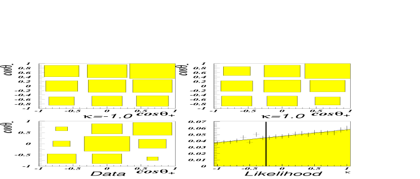
Figure 2: Spin correlation results. The top two plots are Monte Carlo simulations for $\kappa=\pm 1$. The lower left plot shows the data. We fit the data to the Monte Carlo expectations to derive a likelihood as a function of $\kappa$, as plotted in the lower right.

We have six dilepton candidates, with an expected background of $1.5\pm 0.3$ events. For each event, we find the distribution of solutions in $(\theta_{+},\theta_{-})$ and bin it into a 2D histogram. We then sum over all events. The result is shown in Fig. 2. Although the statistics from Run 1 are not sufficient to provide a significant measurement of $\kappa$,we find that $\kappa>-0.25$, at $68\%$ confidence.

This result will improve greatly during the next collider run, where we expect about 150 $t{\bar{t}}{\rightarrow}\hbox{dilepton}$ events. We should be able to discriminate between $\kappa=0$ and $\kappa=+1$ at least at the $2.5\sigma$ level, using just the dilepton channel.

3 Charged Higgs boson search

The SM contains a single complex Higgs doublet, giving rise to a single physical Higgs boson, $H^{0}$. But one can also consider extensions to multiple Higgs doublets, as required by supersymmetry [hhguide]. With two Higgs doublets, there are five physical Higgs bosons, of which two are charged: $H^{0}$, $h^{0}$, $A^{0}$, $H^{+}$, and $H^{-}$. The electroweak sector is then specified by the parameters $m_{W}$, ${m_{H^{+}}}$, and $\tan\beta$, where $\tan\beta$ is the ratio of the vacuum expectation values from the two doublets. If ${m_{H^{+}}}<m_{t}-m_{b}$, then the decay $t{\rightarrow}H^{+}b$ can compete with the SM decay $t{\rightarrow}Wb$.

Figure 3: Map of the $({m_{H^{+}}},\tan\beta)$ parameter space; regions with ${\rm BR}(t{\rightarrow}H^{+}b)>0.5$ are hatched. The charged Higgs decay modes in those regions are also shown. Regions with ${\rm BR}(t{\rightarrow}H^{+}b)>0.9$ (dark shaded regions) are not considered.

Figure 4: $95\%$ C.L. exclusion contours for charged Higgs production for $m_{t}=175\mathop{\hbox{GeV}}\mathclose{}\mathord{}\kern-1.7pt/\kern-1.7ptc^{2}$ and $\sigma(t{\bar{t}})=5.5\mathop{\hbox{pb}}\mathclose{}\mathord{}$ (hatched area, solid lines), $5.0\mathop{\hbox{pb}}\mathclose{}\mathord{}$ (dashed lines), and $4.5\mathop{\hbox{pb}}\mathclose{}\mathord{}$ (dotted lines).

The regions in parameter space where our analysis is sensitive are those where ${\rm BR}(t{\rightarrow}H^{+})$ is large. Those are the regions where ${m_{H^{+}}}$ is low, and $\tan\beta$ is either large or small (see Fig. 3). Once an $H^{+}$ is produced, it can decay in several ways. For large $\tan\beta$, the decay $H^{+}{\rightarrow}\tau\nu$ dominates, while for small $\tan\beta$, $H^{+}{\rightarrow}cs$ is favored. But for $\tan\beta$ small and $m_{H^{+}}$ large, there is an additional decay mode that becomes important: $H^{+}{\rightarrow}t^{*}b{\rightarrow}Wbb$.

We have searched for $t{\rightarrow}H^{+}$ using a “disappearance analysis” [d0chhiggsprl]. This is based on the results of our cross section measurement in the lepton+jets channel [d0xsecprl97]; that is, where one top quark in a pair decays via $t{\rightarrow}bl\nu$ and the other decays via $t{\rightarrow}bqq$. In this channel, we find 30 $t{\bar{t}}$ candidates, with an expected background of $11\pm 2$ events. Assuming that the $t{\bar{t}}$ cross section has no contributions from any new physics channels, we can exclude regions of parameter space in which $t{\bar{t}}$ pairs decay via $H^{+}$ to final states for which our event selection has very low acceptance. In these regions, the observed excess of signal over background cannot be explained by $t{\bar{t}}$ production. The result is shown in Fig. 4, for three assumed $t{\bar{t}}$ cross sections. Note that this analysis is valid only for the interior of the plot. LEP excludes $M_{H^{+}}<60\mathop{\hbox{GeV}}\mathclose{}\mathord{}\kern-1.7pt/\kern-1.7ptc^{2}$, while in the other regions outside the plot, the perturbative calculations for the Higgs branching ratios become invalid. For Run 2, we expect to be able to increase the area excluded by over a factor of two.

4 Neural network analysis of $t{\bar{t}}{\rightarrow}e\mu$

The “golden” channel for the observation of $t{\bar{t}}$ production is $t{\bar{t}}{\rightarrow}e\mu b{\bar{b}}\nu\nu$. Due to the presence of two unlike flavor leptons, this channel has very low background. But its branching fraction is also a small $2.5\%$. It is therefore important to maximize the acceptance in this channel.

For our published measurement [d0xsecprl97], we required one electron with $E_{T}>15\mathop{\hbox{GeV}}\mathclose{}\mathord{}$, one muon with ${p_{\scriptscriptstyle T}}>15\mathop{\hbox{GeV}}\mathclose{}\mathord{}\kern-1.7pt/\kern-1.7ptc$, $\hbox{$E$\hbox to0.0pt{\kern-6.00006pt\raise 0.54668pt\hbox{/}\hss}}_{T}>20\mathop{\hbox{GeV}}\mathclose{}\mathord{}$, two jets with $E_{T}>20\mathop{\hbox{GeV}}\mathclose{}\mathord{}$, $\Delta R(e,{\rm jet})>0.5$ [$(\eta,\phi)$ space], $\Delta R(e,\mu)>0.25$, and $H_{T}\equiv E_{T}^{e}+\sum E_{T}^{{\rm jet}}>120\mathop{\hbox{GeV}}\mathclose{}\mathord{}$. For our new analysis [happythesis], we remove the $H_{T}$ requirement and reduce the jet $E_{T}$ and $\hbox{$E$\hbox to0.0pt{\kern-6.00006pt\raise 0.54668pt\hbox{/}\hss}}_{T}$ requirements to $15\mathop{\hbox{GeV}}\mathclose{}\mathord{}$. To regain background rejection, we turn to a neural network analysis.

Figure 5: Distributions of input variables to the $\tau\tau$ neural network for signal (dashed) and $Z{\rightarrow}\tau\tau$ background (solid). Units are in $\mathop{\hbox{GeV}}\mathclose{}\mathord{}$, except for the last plot.

There are three major backgrounds: QCD jet production, $Z{\rightarrow}\tau\tau{\rightarrow}e\mu$, and $WW{\rightarrow}e\mu$. A separate network is trained to discriminate the signal from each of the three backgrounds. Six variables are used as inputs to each of the networks, these being $E_{T}^{e}$, $E_{T}^{{\rm jet}2}$, $\hbox{$E$\hbox to0.0pt{\kern-6.00006pt\raise 0.54668pt\hbox{/}\hss}}_{T}$, $H_{T}^{{\rm jets}}\equiv\sum_{{\rm jets}}E_{T}^{{\rm jet}}$, $M_{e\mu}$, and $\Delta\phi_{e\mu}$, except for the $\tau\tau$ network, where $E_{T}^{{\rm jet}1}$ replaces $E_{T}^{{\rm jet}2}$. (See Fig. 5.) Each of the networks has seven hidden units, and is trained on equal numbers of $t{\bar{t}}$ signal and background events (4000 events for QCD, and 2000 for the other two). The outputs $O_{{\rm NN}i}$ are combined using $O_{{\rm NN}}^{{\rm comb}}=3/\sum_{i=1}^{3}1/O_{{\rm NN}i}$. (See Fig. 6.) The candidate sample is defined by $O_{{\rm NN}}^{{\rm comb}}>0.88$, determined by maximizing the expected relative significance $S/\sigma_{B}$. ($\sigma_{B}$ is the uncertainty in the background.)

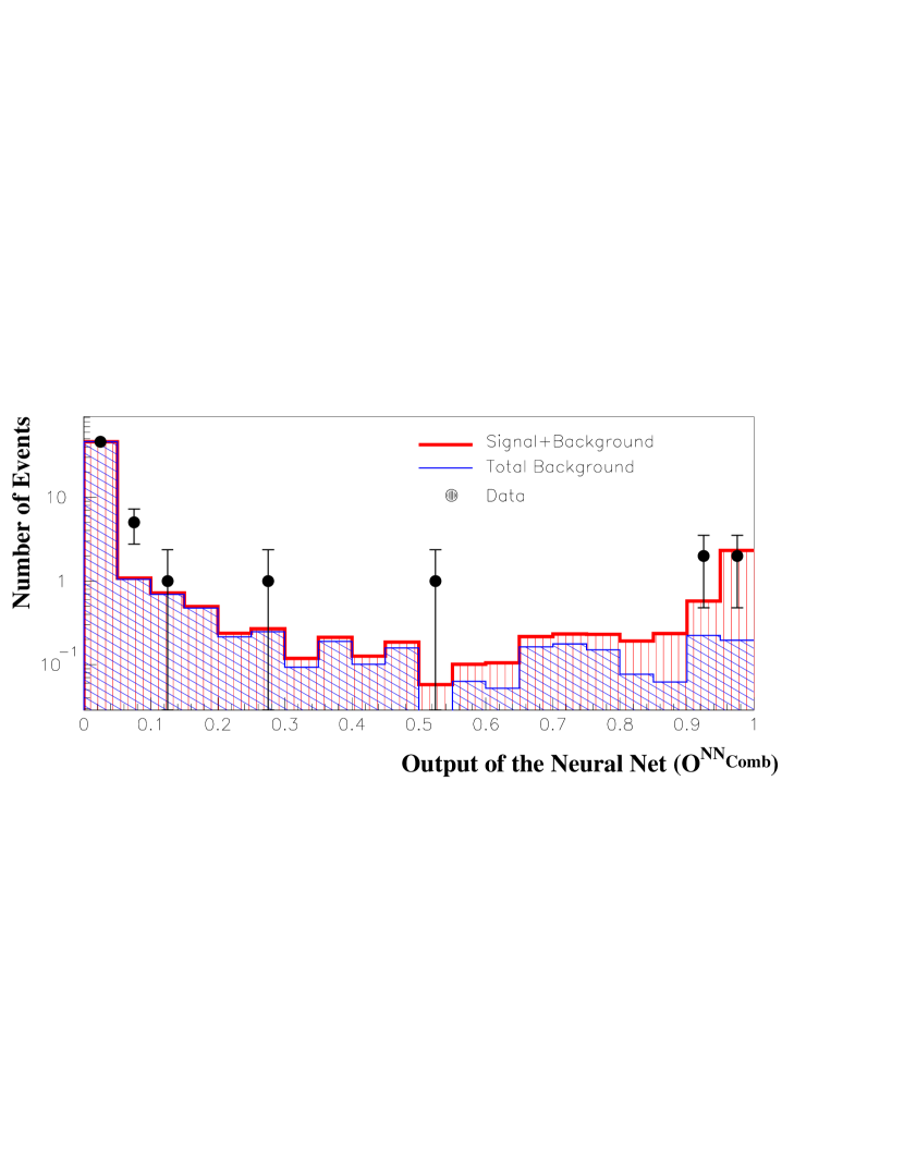
Figure 6: $O_{{\rm NN}}^{{\rm comb}}$ for data, expected background, and expected signal plus background. The events below the signal region have a distribution consistent with background.

The results are shown in Table 1. Compared to the published analysis, the neural network analysis increases the efficiency by about $10\%$. The background is also slightly lower, but this is harder to evaluate due its large statistical uncertainty.

	NN Analysis	Conventional
$\epsilon\times\hbox{BR}$ (%)	$0.402\pm 0.085$	$0.368\pm 0.078$
Background	$0.24\pm 0.15$	$0.26\pm 0.16$
Events observed	$4$	$3$
$\sigma(t{\bar{t}})$	$8.8\pm 5.1\mathop{\hbox{pb}}\mathclose{}\mathord{}$	$7.1\pm 4.8\mathop{\hbox{pb}}\mathclose{}\mathord{}$

Table 1: A comparison of the results of the conventional and neural network $t{\bar{t}}{\rightarrow}e\mu$ analyses, for $m_{t}=175\mathop{\hbox{GeV}}\mathclose{}\mathord{}\kern-1.7pt/\kern-1.7ptc^{2}$. Note that the quoted uncertainties are highly correlated between the two analyses.

References

- [1] \orig@bibitemreview P. Bhat, H. Prosper, and S. Snyder, Int. J. Mod. Phys. A13, 5113 (1998).\orig@bibitemstelzer96 T. Stelzer and S. Willenbrock, Phys. Lett. B374, 169 (1996); K. Y. Lee, H. S. Song, J. Song, and C. Yu, Report No. SNUTP-99-022 (1999), hep-ph/9905227; G. Mahlon and S. Parke, Phys. Rev. D53, 4886 (1996).\orig@bibitemmahlon97 G. Mahlon and S. Parke, Phys. Lett. B411, 173 (1997).\orig@bibitemsuyongthesis S. Choi, Ph.D. thesis, Seoul National University, Seoul, Korea, 1999.\orig@bibitemd0llmassprd DØ Collaboration (B. Abbott et al.), Phys. Rev. D60, 052001 (1999).\orig@bibitemhhguide J. F. Gunion, H. E. Haber, G. Kane, and S. Dawson, The Higgs Hunter’s Guide (Addison-Wesley, New York, 1990).\orig@bibitemd0chhiggsprl DØ Collaboration (B. Abbott et al.), Phys. Rev. Lett. 82, 4975 (1999).\orig@bibitemd0xsecprl97 DØ Collaboration (S. Abachi et al.), Phys. Rev. Lett. 79, 1203 (1997).\orig@bibitemhappythesis H. Singh, Ph.D. thesis, University of California Riverside, Riverside, 1999.