TUHEP-99-06 PDK-743 Search for Nucleon Decay into
Lepton $+$ K⁰ Final States Using Soudan 2

Abstract

A search for nucleon decay into two–body final states containing K⁰ mesons has been conducted using the 963 metric ton Soudan 2 iron tracking calorimeter. The topologies, ionizations, and kinematics of contained events recorded in a 5.52 kiloton-year total exposure (4.41 kton-year fiducial volume exposure) are examined for compatibility with nucleon decays in an iron medium. For proton decay into the fully visible final states $\mu^{+}$K${}^{0}_{s}$ and e⁺K${}^{0}_{s}$, zero and one event candidates are observed respectively. The lifetime lower limits ($\tau/B$) thus implied are $1.5\times 10^{32}$ years and $1.2\times 10^{32}$ years, respectively. Lifetime lower limits are also reported for proton decay into $\ell^{+}$K${}^{0}_{l}$, and for neutron decay into $\nu$K${}^{0}_{s}$.

I Introduction

A SUSY predictions for nucleon decay

Supersymmetry (SUSY) proposes the existence, presumably at high mass scales, of a new fermion or boson partner for each boson or fermion encompassed by the Standard Model. At the expense of doubling the number of elementary particles, SUSY Grand Unified Theories (GUTs) provide a natural solution to the hierarchy problem, allow the extrapolations of the running coupling constants (which have now been precisely determined at low energies and electroweak unification scales) to converge at a high energy scale, make accurate predictions of the Weinberg angle, and incorporate gravitation when locally gauged [1, 2, 3, 4].

Supersymmetric GUTs, such as SUSY SU(5), permit the same processes for nucleon decay as do their non-supersymmetric counterparts; however, the larger mass requirements for the GUT–scale lepto-quark bosons generally preclude the possibility of observing nucleon decay with lifetime divided by branching ratio $\tau$/B of less than $\sim 10^{33}$ years. Interestingly, other processes involving supersymmetric particle loops arise that can mediate nucleon decay. An example is shown in Fig. 1 wherein the decay is suppressed by the product of the color triplet Higgsino and Wino masses rather than by the supersymmetric version of the X and Y lepto-quark bosons [5, 6]. Nucleon decay diagrams of this type give integrals that vanish unless the transitions involve intergenerational mixing. Consequently, final states containing strange mesons are to be expected, with lifetimes predicted to be $\sim 10^{31}-10^{32}$ years [7, 8].

Table I lists some proposed SUSY theories along with their predicted decay modes of leading branching ratios and their lifetime predictions. The expectation that two–body decays yielding a positive–strangeness $K$ meson are predominant, is seen to be a common theme.

B Previous experimental searches for $K^{0}$ modes

Experimental searches for baryon instability in general and for nucleon decay into two-body modes containing K-mesons in particular, have been carried out for more than two decades. Among the early searches which included strangeness modes were the planar iron tracking calorimeter experiments of KGF [13, 14], NUSEX [15], and Soudan 1 [16]. Lifetime lower limits and also observation of a few nucleon decay candidate events, were reported. Among candidate sightings was a three-prong event recorded by NUSEX having kinematics compatible with

$${\rm p}\rightarrow\mu^{+}{\rm K}^{0}{\textstyle,~{}~{}}{\rm K}^{0}_{s}\rightarrow\pi^{+}\pi^{-}.$$ (1)

With more exposure however, this candidate was found to be consistent with background arising from interactions of atmospheric neutrinos within the NUSEX calorimeter.

Lifetime lower limits for proton decay (1) (but including the K${}^{0}_{s}\rightarrow\pi^{0}\pi^{0}$ mode) and for neutron decay

$${\rm n}\rightarrow\nu{\rm K}^{0}{\textstyle,~{}~{}}{\rm K}^{0}_{s}\rightarrow\pi^{0}\pi^{0}.$$ (2)

were reported by the IMB water Cherenkov experiment in 1984 [17]. These limits were improved upon and the scope of search extended to other K-meson modes in subsequent investigations by IMB [18, 19, 20]. Lifetime limits were also obtained with the HPW water Cherenkov detector [21]. More recently, nucleon decay limits for many modes have been published, including the K⁰ modes considered in the present work, based upon the 7.6 kton-year exposure recorded by IMB-3[22].

Nucleon decays involving K⁰ and K⁺ mesons were searched for using the iron tracking calorimeter experiment of the Frejus collaboration; lifetime lower limits are reported in Refs. [23, 24, 25]. Among the highest of published lifetime lower limits for lepton plus kaon two-body modes are the 1989 results by the Kamiokande water Cherenkov experiment [26] based upon a 3.76 kton year exposure of KAM-I and KAM-II.

A search for the proton decay mode p $\rightarrow\nu$K⁺ in the Soudan 2 experiment has been reported in a previous publication [27]. A more stringent lifetime limit for this mode has recently been published by Super-Kamiokande [28]. In this work we report our search in Soudan 2 for nucleon decay into two–body modes involving K⁰ mesons, namely proton decay into $\mu^{+}$K⁰ and e⁺K⁰ with K${}^{0}\rightarrow$ K${}^{0}_{s}$ or K${}^{0}_{l}$, and neutron decay into $\nu$K${}^{0}_{s}$. Soudan 2 has the capability to observe these leading SUSY decays if indeed their lifetimes are within the ranges indicated in Table I.

II Detector and Event Samples

A Tracking calorimeter and active shield

Soudan 2 is a 963 metric ton iron tracking calorimeter which is currently taking data. It is located at a depth of 2340 ft (2070 mwe) on the 27th level of the Soudan Underground Mine State Park in northern Minnesota. Data–taking commenced in April 1989 when the detector’s total mass was 275 tons. The modular design allowed data-taking to proceed while additional 4.3-ton calorimeter modules were being installed. The detector was completed in November 1993 at 963 tons. The total (fiducial) exposure analyzed here is 5.52 (4.41) kiloton–years (kty), obtained from data–taking through October 1998.

Each of the 224 modules that comprise the calorimeter consists of layered, corrugated iron sheets instrumented with drift tubes which are filled with an Argon–CO₂ gas mixture. Electrons liberated by incident ionizing particles drift to the ends of the tubes under the influence of an electric field sustained by a voltage gradient which is applied along the tubes. The drifted charge is collected by vertical anode wires held at a high voltage, while horizontal cathode pad strips register the image charges. Two of the position coordinates of the ionized track segments are determined by identifying the anode wire and cathode pad strips excited; the third coordinate is determined from the drift–time of the liberated charge once the event “start time” has been determined [29, 30].

Surrounding the tracking calorimeter but mounted on the cavern walls and well separated from calorimeter surfaces, is the 1700 m² active shield array comprised of 2 – 3 layers of proportional tubes [31]. The shield enables us to identify events which are not fully contained within the calorimeter. In particular, it provides tagging of background events initiated by cosmic ray muons, as will be described in sections II B and II D below.

In searches for nucleon decay into multiprong modes, the Soudan 2 iron tracking calorimeter of honeycomb lattice geometry offers event imaging capabilities heretofore not achieved by the planar iron calorimeter experiments or by the water Cherenkov experiments. For the multiprong events of this work, Soudan’s fine–grained tracking enables event vertex locations to be established to within 0 to 3 cm in the anode or cathode coordinate (drift-time coordinate) relative to the honeycomb stack (to the rest of the event). This spatial resolution enables discrimination, based upon proximity to the event vertex, between a prompt e^± shower and a photon initiated shower. In Soudan 2, ionizing particles having non-relativistic as well as relativistic momenta are imaged with $dE/dx$ sampling. Consequently, final state topologies are more completely ascertained, and proton tracks can be distinguished from charged pion and muon tracks. These capabilities are valuable for rejection of background.

B Event samples

Events used in this analysis are required to be fully contained within a fiducial volume, defined to be the 770-metric-ton portion of the calorimeter which is everywhere more than 20 cm from all outer surfaces. There are four distinct samples which are either simulated (Monte Carlo events) or collected (data events) :

1. i) We use full detector nucleon decay Monte Carlo simulations, including detector noise, to generate samples of the various nucleon decay processes considered in this work. Hereafter we refer to these events as nucleon decay MC events. Details concerning generation and utilization of such events are given in Ref. [27].

2. ii) A full detector neutrino Monte Carlo (MC) simulation, which includes detector noise, is used to generate events representing all charged-current and neutral-current reactions which can be initiated by the flux of atmospheric neutrinos. These neutrino MC events are injected into the data stream prior to physicist scanning and are subsequently processed and evaluated using the same procedures as used with the data events. The Monte Carlo program is based upon the flux predictions of Barr, Gaisser, and Stanev [34, 35] and is described in a previous Soudan 2 publication [32]. Among the neutrino reactions simulated, care has been taken to include K⁰/$\overline{\rm K}^{0}$ channels; these arise at low rate from $\Delta S=0$ associated production and from $\Delta S=1$ processes [36]. All of the atmospheric neutrino MC samples in this paper correspond to a fiducial detector exposure of 24.0 kton-years.

3. iii) There are contained events for which the veto shield registered coincident, double–layer hits. Such events usually originate with inelastic interactions of cosmic ray muons within the cavern rock surrounding the detector. The muon interactions eject charged and neutral particles out of the rock and into the calorimeter; these particles subsequently interact to make events in the detector. On rare occasions there can be cosmic ray induced events which are unaccompanied by coincident hits in the active shield; these arise either from shield inefficiency or from instances wherein a neutron or photon with no accompanying charged particles emerged from the cavern walls. Contained events of cosmic ray origin are hereafter referred to as “rock events”; these can be “shield–tagged” or otherwise of the “zero–shield–hit” variety.

4. iv) The “gold events” are data events for which the cavern–liner active shield array registered no signal during the event’s allowed time window. These events are mostly interactions of atmospheric neutrinos [32].

C Processing of events

Each event included in a contained event sample for physics analysis has passed through a standard data reduction chain. Care has been taken to ensure that both data and Monte Carlo simulation events pass through the same steps in the chain. For an event to be recorded, the central detector requires at least seven contiguous pulse “edges” to occur within a 72 $\mu$s window before a trigger is registered and the calorimeter modules are read out. For MC events, the requirements of the hardware trigger are imposed by a trigger simulation code. All events, data and Monte Carlo, are then subjected to a containment filter code, which rejects events for which part of the event extends outside the fiducial volume. Taken together, the trigger and containment filter requirements will typically reduce a sample of MC nucleon decay events by 35% to 65%, depending upon the decay mode being investigated.

Events which survive the trigger and containment requirements, whether they be data events (gold or rock) or Monte Carlo (neutrino reaction or nucleon decay), are then subjected to two successive “scanning passes” carried out by physicists [32]. Each scanning pass involves three independent scans. In the first pass, multiprong events are found with an overall multiple-scan efficiency of $0.98^{+0.02}_{-0.04}$ [33]. The first scan pass is designed to ensure event quality. Here, residual uncontained events that have not been rejected by the software filter are eliminated. Noise events, and events that have prongs ending on detector cracks are also rejected at this stage. In the second scanning pass, broad topology assignments are made (track or shower – with or without a visible recoil proton, single proton and multiprong) and an additional level of scrutiny with regard to containment is provided. Multiprong events that survive both scanning passes are then subjected to detailed topology assignment.

Once topologies have been assigned, events are reconstructed using software tools available within our interactive graphics package. Tracks are fitted using a routine that fits a polynomial curve through all hits selected and returns the range, energy and initial direction vector. There is also a shower processing routine which determines the energy and initial direction vector for clusters of hits that are tagged as showers. The collection of reconstructed tracks and showers along with mass hypotheses for the tracks is then written into a data summary file, from which the derived quantities such as event energy, invariant mass, net event momentum, etc., can be determined. As a measure of event resolution, we calculate the difference between Monte Carlo truth and the reconstructed final-state energy. The resulting $\Delta E/E$ values for fully-visible final states are ($19\pm 2$) % for multiprongs with prompt muons, and ($28\pm 2$) % for multiprongs with prompt electrons. These values characterize reconstruction for nucleon decay ($\ell^{+}$ + hadrons) events and for $\nu_{\ell}$ charged-current multiprongs near threshold.

The fractions of event samples which remain after successive application of each of the above-mentioned selections, averaged over the full volume of the detector, are given in Table II for each nucleon decay mode of this study. For each nucleon decay mode with a particular daughter process, a sample of 493 MC events was generated. For the K${}^{0}_{l}$ modes, the portions of the MC samples which pass all cuts except the kinematic ones are given by the top row, leftmost entries of Tables III and IV.

D Cosmic ray induced background in “gold” data

The gold data events analyzed in this work are multiprong events which are mostly neutrino-induced, however a small number may arise from rock events which are unaccompanied by hits in the veto shield array. The latter events are initiated by neutrons emerging from the cavern rock which are incident upon the calorimeter. In contrast to neutrino interactions (or nucleon decay) which distribute uniformly throughout the calorimeter volume, these events tend to occur at relatively shallow depth into the detector.

Our estimate of the number of zero-shield-hit rock events in multiprong data is based upon a multivariate discriminant analysis of the gold data, neutrino MC, and shield-tagged rock samples[37]. For this analysis, discriminant functions characterizing each sample are constructed using five event variables (of which several are highly correlated). These include: i) Penetration depth, measured along the event net momentum, ii) vertex distance to the closest exterior surface, iii) event visible energy, iv) zenith angle of the net momentum vector, and v) “inwardness”, defined as the cosine between event $\vec{p}_{net}$ and the unit normal, pointing inward, of the closest exterior surface of the calorimeter. By fitting the discriminant variable distribution from gold data to a combination of neutrino MC and rock discriminant distributions, the zero-shield-hit rock contribution is ascertained. Out of the total number of multiprong rock events (with and without shield hits), the fraction of events having shield hits is $f=0.94\pm 0.04$. Among 144 gold data multiprongs, $16\pm 11$ events may be cosmic-ray induced. Approximately 30% of the zero-shield-hit rock rate can be ascribed to inefficiency of the shield array.

For each nucleon decay channel, we subject the shield-tagged rock multiprongs to the same selection cuts which are applied to data multiprongs. The number of zero-shield-hit rock events which are background for the channel is then calculated as the product $(1-f)/f$ times the number of shield-tagged rock events which pass the cuts.

E Neutrino background rates and atmospheric $\nu_{\mu}$ oscillations

In calculating event rates for neutrino-induced background in a nucleon decay search, a consideration arises with the well-known discrepancy between the observed versus predicted flavor ratio $\nu_{\mu}/\nu_{e}$ for atmospheric neutrinos. In single track and single shower events, Soudan 2 observes the ratio-of-ratios ($\nu_{\mu}/\nu_{e}$ observed/expected) to be 0.64 $\pm$ 0.11 (stat.) $\pm$ 0.06 (syst.) [45]. From the exposure analyzed for this work, we estimate $128\pm 14$ contained multiprong events to be neutrino events, where the uncertainty is the quadrature sum of statistical error and an error from the rock background subtraction. This can be compared to the number of neutrino-induced multiprong events predicted by the null oscillation Monte Carlo: $154\pm 6$ events, where the uncertainty represents statistical error from the atmospheric neutrino simulation. The difference may be accounted for by atmospheric neutrino oscillations $\nu_{\mu}$ to $\nu_{x}$. In any case, evidence for depletion of the atmospheric muon-neutrino flux is sufficiently extensive [46] that an accounting of the effect in nucleon decay background rates is warranted.

The basis for our atmospheric neutrino background estimates is our realistic MC simulation which uses null oscillation fluxes. The disappearance of $\nu_{\mu}$-flavor neutrinos resulting from $\nu_{\mu}\rightarrow\nu_{x}$ oscillations, affects backgrounds initiated by $(\nu_{\mu}+\overline{\nu}_{\mu})$ charged-current reactions; in fact, it reduces this background component. In implementing our correction we further assume, as indicated by recent data, that $\nu_{x}$ is an active neutrino which is not $\nu_{e}$ (i.e. $\nu_{x}=\nu_{\tau}$) [47]. Then, the predominant atmospheric neutrino oscillation does not affect background arising from charged-current reactions of $\nu_{e}$-flavor neutrinos, nor does it affect background from neutral currents. Consequently, to correct for $\nu_{\mu}$-flavor disappearance, the number of $(\nu_{\mu}+\overline{\nu}_{\mu})$ charged-current background events estimated from the atmospheric-neutrino MC for each nucleon decay channel, has been scaled by the flavor ratio 0.64 $\pm$ 0.13.

As described below, the neutrino background is very low in the proton decay channels p $\rightarrow\mu^{+}{\rm K}^{0}_{s}$, K${}^{0}_{s}\rightarrow\pi^{+}\pi^{-}$ and p $\rightarrow\mu^{+}{\rm K}^{0}_{l}$. In most other channels, e.g. p $\rightarrow\mu^{+}{\rm K}^{0}_{s}$, K${}^{0}_{s}\rightarrow\pi^{0}\pi^{0}$, p $\rightarrow{\rm e}^{+}{\rm K}^{0}_{s}$, p $\rightarrow{\rm e}^{+}{\rm K}^{0}_{l}$, and n $\rightarrow\nu{\rm K}^{0}_{s}$, K${}^{0}_{s}\rightarrow\pi^{0}\pi^{0}$, the neutrino background is either low or otherwise dominated by $\nu_{e}$ flavor reactions. In fact, the only decay channel in this work for which $\nu_{\mu}$-flavor disappearance has a significant effect on the lifetime lower limit is neutron decay n $\rightarrow\nu{\rm K}^{0}_{s}$, K${}^{0}_{s}\rightarrow\pi^{+}\pi^{-}$. For this particular channel, backgrounds and corresponding lifetime lower limits are presented both with and without correction for $\nu_{\mu}$ oscillations.

III Characterization of Nucleon Decay Reactions

For each nucleon decay mode, a Monte Carlo sample is created and processed as described in Section II; similarly handled are the gold data, the contained shield-tagged rock events, and the atmospheric neutrino MC events. These samples are used to determine the topological and kinematic properties that differentiate each nucleon decay mode from other modes and from the atmospheric neutrino and the rock event backgrounds.

A Event generation

For each nucleon decay mode, five hundred events are typically generated throughout the full detector volume. They are then overlaid onto pulser trigger events which sample the detector background noise (from natural radioactivity and cosmic rays) at regular intervals throughout the exposure. The effects of Fermi motion within the iron and other nuclei which comprise the detector are taken into account in simulation using the parametrization of Ref. [38]. For two–body nucleon decays in which the final state momenta would otherwise be unique, Fermi motion smears the momenta and thereby complicates final state identification.

For final states from neutrino interactions and also from nucleon decay wherein pions are directly produced, intranuclear rescattering is treated in our Monte Carlo using a phenomenological cascade model [39]. Parameters of the model, which scale with $A$, are set by requiring that threshold pion production observed in $\nu_{\mu}$–deuteron ($A=2$) and $\nu_{\mu}$–neon ($A=20$) reactions be reproduced [40]. For K⁰ mesons however, inelastic intranuclear rescattering is expected to be small due to the absence of low–lying K⁰N ($S=+1$) resonances and is not simulated.

B Final state kinematics

We examined each simulated nucleon decay mode for kinematic characteristics which are suitable for selection of data candidates and for separation of backgrounds. Two quantities that are generally useful are the invariant mass, $M_{inv}$, and the magnitude of the net three–momentum, $\left|\vec{p}_{net}\right|$, of reconstructed final state particles. For the distribution in either variable, there is an expectation which can be simulated using the nucleon decay MC events. For modes in which all final state particles are visible, the invariant mass should fall in a range about the nucleon mass (less 8 MeV binding energy) whose width is determined by the resolution of the detector.

If some final state particles are not observable, useful information can still be extracted from the invariant mass. For example, in the case of n $\rightarrow\overline{\nu}$K${}^{0}_{s}$ the mass will correspond to that of the reconstructed K${}^{0}_{s}$. The nominal 338 MeV/$c$ K⁰ momentum from this two-body decay will be boosted by the Fermi motion of the decaying neutron and smeared further by detector resolution.

C Selection contour in the $\textstyle M_{inv}$ versus $\textstyle\left|\vec{p}_{net}\right|$ plane

A scatter plot of invariant mass versus net event momentum can be created for the reconstructed final states for each simulation. A region in this plane can be chosen whose boundary defines a kinematical selection which can be applied to the data and to the background samples. For our searches we consider the application of such a cut to be the “primary constraint” and we have formulated a quantitative parameterization of this two–variable constraint. We observe that the final-state invariant mass exhibits a distribution which is Gaussian to a good approximation. Similarly, the final-state net momentum magnitude which results from the folding of Fermi motion with the experimental resolution, distributes with a shape which is very nearly Gaussian. Consequently, the density distribution of points on the invariant mass versus momentum plane can be fitted by a bi–variate Gaussian probability distribution function. In principle, when the correlation coefficient is set to zero, the form of the fitting function should be

$$Z_{\alpha\beta}\left(x,y\right)=\frac{1}{2\pi\sqrt{\sigma_{\alpha}\sigma_{\beta}}}e^{-\frac{1}{2}\left[\left(\frac{x-\mu_{\alpha}}{\sigma_{\alpha}}\right)^{2}+\left(\frac{y-\mu_{\beta}}{\sigma_{\beta}}\right)^{2}\right]}$$ (3)

where $\sigma_{\alpha}$ and $\sigma_{\beta}$ are the widths and $\mu_{\alpha}$ and $\mu_{\beta}$ are the means of the two distributions. In practice however, the conic section may have semimajor and semiminor axes that are not parallel to the ordinate and abscissa of the graph. To allow such a rotation on the plane, a new basis (which is a linear combination of the old variables) is constructed with the new mean and widths defined on that basis. The form of the fitting function then becomes

$$Z_{\alpha\beta}\left(x,y\right)=Ae^{-\frac{1}{2}\left[\left(\frac{ax+by-\mu_{\alpha}}{\sigma_{\alpha}}\right)^{2}+\left(\frac{ay-bx-\mu_{\beta}}{\sigma_{\beta}}\right)^{2}\right]}.$$ (4)

Note that the two arguments of the exponentials are formulated to be mutually perpendicular lines which, when fit, will be collinear with the major and minor axes of the elliptical contours of the sections of the Gaussian surface.

For each mode in which this representation of a density distribution is used, a lego plot for the simulation is created (see Fig. 2a). The seven–parameter function above is fitted to the simulation using a log-likelihood ${\chi}^{2}$ minimization routine available in the MINUIT software package (see Fig. 2b and Fig. 3). The bi-variate Gaussian form (Eq. 4) was found to provide a good fit to the nucleon decay event density distribution in every case, with $\chi^{2}$ per degree of freedom (dof) values in the range 0.7 to 1.3.

The projection of the bi-variate Gaussian surface of Fig. 2b onto the $M_{inv}$ versus $\left|\vec{p}_{net}\right|$ plane is shown in Fig. 3. Here, the shape of the event distribution over the plane is depicted using five nested, elliptical contour boundaries. Proceeding outward from the innermost contour, the bounded regions contain respectively 10%, 30%, 50%, 70%, and 90% of the event sample. From the five regions delineated, we choose the 90%-of-sample contour - the outermost, solid curve ellipse in Fig. 3 - for quantitative use in nucleon decay searches of this study. In particular, for p $\rightarrow\ell^{+}{\rm K}^{0}_{s}$ searches we take this outermost contour to define our “primary” kinematic selection, namely: A candidate proton decay event must have reconstructed ($M_{inv}$, $\left|\vec{p}_{net}\right|$) values which lie within the contour boundary. Concerning the interior contours (dashed ellipses of Fig. 3), no quantitative utilization will be made. However, by superposing event coordinates onto a contour set such as shown in Fig. 3, a degree of insight is afforded as to whether an event sample as a whole exhibits the kinematics of nucleon decay. For this reason we display interior contours along with the 90% contour in various kinematic diplots of this study.

D Other kinematic selection contours

The kinematic requirement on final-state invariant mass versus net momentum combinations which the outermost contour of Fig. 3 represents, is a constraint which nucleon decay will satisfy but which background processes need not respect. The background rejection thus afforded can be augmented using contours constructed with other kinematic variables.

From trials with Monte Carlo event samples we find that, with procedures to be described below, the final-state lepton prong can be identified with near certainty (in final states e⁺($\pi^{+}\pi^{-}$) and $\mu^{+}$($\pi^{0}\pi^{0}$)) or with useful efficiency (84% for $\mu^{+}$($\pi^{+}\pi^{-}$) and 82% for e⁺($\pi^{0}\pi^{0}$)). With this identification in place, a distinction can be made between the lepton and the K${}^{0}_{s}$ system. (Unfortunately, the neutral track gap produced by the moving K${}^{0}_{s}$ is usually not large enough to be resolved in the Soudan 2 calorimeter.) Then, the kinematics allowed for the K${}^{0}_{s}$ subsystem of proton decay can usefully be specified by a contour boundary in the plane of K${}^{0}_{s}$ invariant mass versus K${}^{0}_{s}$ momentum. A further kinematic restriction on momentum-sharing between the lepton and the K${}^{0}_{s}$ can also be formulated (albeit mostly redundant with constraints already mentioned) in terms of an allowed contour region in the lepton momentum versus K${}^{0}_{s}$ momentum plane.

One might expect that reconstruction of the charged pion tracks in p $\rightarrow\ell^{+}$K${}^{0}_{s}$ final state with K${}^{0}_{s}\rightarrow\pi^{+}\pi^{-}$ in Monte Carlo samples would on average yield the K⁰ invariant mass. In the Soudan detector, however, scattering processes tend to reduce the range of pion tracks. As a result, our reconstruction of MC event images which is based upon track range, yields an invariant mass distribution with a mean of 461 MeV/$c^{2}$. Also, the momentum distribution of the reconstructed K⁰ is shifted downward by about 50 MeV/$c$.

In our $\ell^{+}$K${}^{0}_{s}$ and $\nu$K${}^{0}_{s}$ searches described below, supplementary requirements are invoked using the above-mentioned additional search contours. Their construction proceeds similarly as with the primary constraint contour of Sect. III C; each contour represents the projection of a bivariate Gaussian fit to the distribution of nucleon decay MC events in two kinematic variables. A data event, in order to qualify as a nucleon decay candidate, must have kinematic coordinates occuring within each contour projection, the boundary of which, by construction, includes the coordinates of 90% of the MC nucleon decay sample.

IV Nucleon decay search

A Search for $\textstyle{\rm p}\rightarrow\mu^{+}{\rm K}^{0}_{s}$ and $\textstyle{\rm p}\rightarrow{\rm e}^{+}{\rm K}^{0}_{s}$

We now consider searches for two–body decay modes $\ell^{+}$K${}^{0}_{s}$, for which the entire final state is observable in Soudan 2. Although the standard SUSY SU(5) GUT models usually predict lifetimes for $\ell^{+}$K⁰ modes to be two orders of magnitude longer than those for $\overline{\nu}$K modes [41], there are other GUT models in which a charged lepton mode could be enhanced [9, 10, 12].

With $\ell^{+}$K${}^{0}_{s}$ modes, the final state will be reconstructed with invariant mass approximating the nucleon mass and with event net momentum within a range compatible with Fermi motion in iron folded with the detector resolution. The kinematically allowed region in the plane of final-state invariant mass versus event net momentum, which is obtained from Soudan reconstructions of Monte Carlo proton decay events, is rather similar for all modes of this kind. As shown in Figure 3 and also in Fig. 4a, we have used simulations involving four separate proton decay modes including K${}^{0}_{s}$, to define a “primary” kinematic selection contour in the $M_{inv}$ versus $\left|\vec{p}_{net}\right|$ plane. That is, for the proton decay searches involving p $\rightarrow\mu^{+}$K${}^{0}_{s}$ and p $\rightarrow$ e⁺K${}^{0}_{s}$, we require all candidate events to have kinematics compatible with the outermost contour depicted in Fig. 4a. As indicated by Figs. 4b, 4c and  4d, the primary contour alone provides a very restrictive kinematic selection.

$\textstyle{\rm p}\rightarrow\mu^{+}{\rm K}^{0}_{s}$

For this mode we examine two topologies: i) three tracks (from K${}^{0}_{s}\rightarrow\pi^{+}\pi^{-}$) and ii) one track plus 3–4 showers (from K${}^{0}_{s}\rightarrow\pi^{0}\pi^{0}$). In the first case, the track which traverses the most calorimeter material and which does not have a visible scatter is taken to be the $\mu^{+}$; the other two tracks are tagged as pions. An illustrative Monte Carlo event of p $\rightarrow\mu^{+}$K${}^{0}_{s}$ with the three–track topology, is shown in Fig. 5. For K${}^{0}_{s}\rightarrow\pi^{0}\pi^{0}$ the lone track is assumed to be the muon, and the showers are reconstructed as the $\pi^{0}\pi^{0}$ system from the K${}^{0}_{s}$. To make optimal use of constraining variables, it is useful and also sufficient to invoke here two distinct kinematic contours. In addition to requiring the primary contour constraint on the final state $M_{inv}$ versus $\left|\vec{p}_{net}\right|$, we require the “K⁰” invariant mass versus momentum to fall within the contour of Fig. 6. The distributions of each of our four event samples (simulation, neutrino MC, rock and data) with respect to the two different kinematic selection contours, for both final states corresponding to p $\rightarrow\mu^{+}$K${}^{0}_{s}$, are summarized in Figures 4 and 6. In Fig. 6, events that failed the preceeding contour cut are shown using open symbols. A candidate event is required to fall within both contours. (Note that events in Fig. 4 can populate overflow regions of Fig. 6, e.g. the track-plus-showers event in Fig. 4d is off-scale in Fig. 6d.)

As a possible addition or alternative to the contour of Fig. 6, event kinematics can be evaluated using a contour in the plane of lepton momentum versus K${}^{0}_{s}$ momentum. For our $\mu^{+}$K${}^{0}_{s}$ search, we find no improvement to be afforded. (For e⁺K${}^{0}_{s}$ however, such a contour provides extra background suppression and we utilize it in that search.)

For the K${}^{0}_{s}\rightarrow\pi^{+}\pi^{-}$ case, the contour cuts are 88% efficient whereas for K${}^{0}_{s}\rightarrow\pi^{0}\pi^{0}$ the combined contour cut efficiency is 80%. The application of these kinematic cuts, together with the branching ratio, software and scanning efficiencies, results in an overall proton-decay survival fraction of $(16\pm 3)$% for the K${}^{0}_{s}\rightarrow\pi^{+}\pi^{-}$ case and $(6\pm 1)$% for K${}^{0}_{s}\rightarrow\pi^{0}\pi^{0}$. No event is observed to satisfy all kinematic constraints for either of the $\pi\pi$ final states.

For the $\mu^{+}$K${}^{0}_{s}$ final state with K${}^{0}_{s}\rightarrow\pi^{0}\pi^{0}$, the estimated neutrino background of 0.6 events is mostly due to $\nu_{e}$ charged-current $\pi^{+}\pi^{0}$ production. No neutrino MC events passed the cuts for the $\mu^{+}{\rm K}^{0}_{s}$ final state with K${}^{0}_{s}\rightarrow\pi^{+}\pi^{-}$; neutrino–induced backgrounds are expected to be low for this case [36].

From our observations of the K${}^{0}_{s}\rightarrow\pi^{+}\pi^{-}$ and $\pi^{0}\pi^{0}$ decay modes, we set a proton decay lifetime limit using the formula [23, 27, 42]

$$\tau/{\textstyle B}({\rm p}\rightarrow\mu^{+}{\rm K}^{0}_{s})>N_{p}\times T_{f}\times\frac{\left[\epsilon_{1}\times{\textstyle B}{{}_{1}}(K)+\epsilon_{2}\times{\textstyle B}{{}_{2}}(K)\right]}{\mu_{1}+\mu_{2}}.$$ (5)

Here $N_{p(n)}=2.87(3.15)\times 10^{32}$ protons (neutrons) in a kiloton of the Soudan 2 detector, $T_{f}=5.52$ kiloton years is the full detector exposure (4.41 kty is the fiducial exposure), and $\epsilon_{i}\times{\textstyle B}{{}_{i}}(K)$ are the selection efficiencies given in Table II. The $\mu_{i}$ are the constrained 90% CL upper limits on the numbers of observed events, and are found by solving the equation

$$0.10=\frac{\sum_{n_{1}=0}^{n_{ev;1}}\sum_{n_{2}=0}^{n_{ev;2}}P(n_{1},b_{1}+\mu_{1})P(n_{2},b_{2}+\mu_{2})}{\sum_{n_{1}=0}^{n_{ev;1}}\sum_{n_{2}=0}^{n_{ev;2}}P(n_{1},b_{1})P(n_{2},b_{2})}$$ (6)

with the constraint

$$\frac{\epsilon_{1}\times{\textstyle B}{{}_{1}}(K)}{\mu_{1}}=\frac{\epsilon_{2}\times{\textstyle B}{{}_{2}}(K)}{\mu_{2}}=\frac{\sum_{i=1}^{2}\epsilon_{i}\times{\textstyle B}{{}_{i}}(K)}{\sum_{i=1}^{2}\mu_{i}}$$ (7)

where $P(n,\mu)$ is the Poisson function, $e^{-\mu}\mu^{n}/n!$, and the $b_{i}$ are the estimated backgrounds. With no candidates found for either $\mu^{+}$K${}^{0}_{s}$ mode, we obtain $\mu_{1}=\mu_{2}=2.31$. The combined lower lifetime limit, at 90% CL and with background subtraction, is then $\tau/{\textstyle B}>150\times 10^{30}$ years.

Our limit for p $\rightarrow\mu^{+}{\rm K}^{0}_{s}$ can be compared to the channel limit previously obtained with the Frejus planar iron calorimeter: $\tau/B>64\times 10^{30}$ years at 90% CL [24]. The water Cherenkov experiments Kamiokande and IMB-3 have reported limits for p $\rightarrow\mu^{+}{\rm K}^{0}$ which are more stringent. Lifetime limits for $\mu^{+}{\rm K}^{0}$ are summarized below, following the discussion of p $\rightarrow\mu^{+}{\rm K}^{0}_{l}$ searches.

$\textstyle{\rm p}\rightarrow{\rm e}^{+}{\rm K}^{0}_{s}$

We examine events which have the following topologies: i) one shower plus two tracks (from K${}^{0}_{s}\rightarrow\pi^{+}\pi^{-}$), or ii) 4 to 6 separate showers (from K${}^{0}_{s}\rightarrow\pi^{0}\pi^{0}$). For p $\rightarrow$ e⁺K${}^{0}_{s}$, three kinematic constraint contours are generated for each of the two daughter modes, and the data events and both backgrounds are subjected to the cuts thus specified (see sections III C and III D). Figure 4 shows the primary contour ($M_{inv}$ vs. $\left|\vec{p}_{net}\right|$) for this case; Fig. 7 shows the final contour (e⁺ momentum versus K${}^{0}_{s}$ momentum) after the K⁰ mass versus K⁰ momentum contour constraint has been applied (the latter contour, not shown, introduces constraints as in Fig 6.). In case ii) with 4–6 showers in the final state, the prompt e⁺ shower must be distinguished from the $\gamma$ showers originating with decaying $\pi^{0}$s. In scanning of candidate events, the shower prong most likely to be the positron is chosen based upon the topology at the primary vertex. The momentum of the shower chosen by the physicist scanner is subsequently compared to the highest momentum among the other showers in the event. If the physicists’ choice is within 50 MeV/$c$ of being the overall shower of highest momentum, it is accepted as the e⁺, otherwise the shower of highest momentum is chosen. In simulation, this algorithm selects the true e⁺ shower in 82% of the events. Again, events that have failed a previous cut are plotted using open symbols. Events considered to be candidates are required to be inside of all three contours.

In the case of the e⁺K${}^{0}_{s}$ final state with K${}^{0}_{s}\rightarrow\pi^{+}\pi^{-}$, the efficiency of all three kinematic selections combined is 86%. The overall efficiency times branching ratio is then 15%. The number of candidates observed is one event whereas the total expected background is 0.74 events. Roughly two-thirds of the expected background comes from $\nu_{e}$ charged-current single charged-pion production events in which the proton is misidentified as another pion.

Fig. 8 shows our single e⁺K${}^{0}_{s}$ candidate in the most orthogonal projection which for this event is the cathode ($Y$) versus drift time ($Z$) projection. A “prompt” electron shower and two tracks are seen to emerge from the primary vertex (denoted MARK 1). The mean pulse height for either track is too low for a proton assignment but is typical for a pion (or muon). The longer pion track traverses an insensitive module-to-module boundary region, giving rise to the apparent gap in the track. The ionization pulse heights on this pion track indicate that the vertex at higher $Y$ is a secondary scatter, not the primary vertex. These pulse heights are smaller (larger) before (after) the proposed scatter point. The kinematics of this event is, however, somewhat atypical for proton decay. In the plane of e⁺ versus K⁰ momentum, this event (depicted by the solid triangle in Fig. 7d) lies within our search contour, but outside the contour which contains 80% of proton decays surviving our selections for this mode. It is of interest to consider the “maximum” number of proton decays which could appear as in Fig. 8 and which are allowed in our exposure, assuming the limits published by Kamiokande, Frejus, and IMB-3 [26, 24, 22] to be correct. Using the range of limit values reported for the e⁺K${}^{0}_{s}$ mode (see below) and the detection efficiency for this channel in the Soudan 2 detector (Table II, third row), of order 0.8 to 3.2 occurrences of proton decay resembling the Fig. 8 candidate would be compatible with previous limits.

For the e⁺K${}^{0}_{s}$ final state with K${}^{0}_{s}\rightarrow\pi^{0}\pi^{0}$, 75% of all simulated proton decay events survive the three kinematic cuts and the overall efficiency times branching ratio for this mode is $(8\pm 1)$%. For this case no data events pass the cuts and 0.63 background events are expected.

Combining the observations from the two separate decay sequences, we obtain for ${\rm p}\rightarrow{\rm e}^{+}{\rm K}^{0}_{s}$ a lifetime lower limit at 90% CL of $\tau/B>120\times 10^{30}$ years. A value of $\tau/B>76\times 10^{30}$ years was reported for this mode previously by Frejus [24]. Limits for e⁺K⁰ are summarized below, following the discussion of p $\rightarrow{\rm e}^{+}{\rm K}^{0}_{l}$ searches.

B Search for $\textstyle{\rm p}\rightarrow\mu^{+}{\rm K}^{0}_{l}$ and $\textstyle{\rm p}\rightarrow{\rm e}^{+}{\rm K}^{0}_{l}$

For proton decay p $\rightarrow\ell^{+}$K⁰, the $K^{0}_{s}$ daughter decays account for half of the possible final states; we now consider p $\rightarrow\ell^{+}$K${}^{0}_{l}$. In these decays the K${}^{0}_{l}$ will interact hadronically in the Soudan 2 medium before it has time to undergo $3\pi$ decay. The event topologies produced by the products of the K${}^{0}_{l}$ interaction are quite varied but are usually easily discernible. The basic topology searched for is that of a single isolated lepton (either $\mu^{+}$ or e⁺), with the appropriate two–body decay momentum, separated from a secondary vertex produced by the hadronic products of the K${}^{0}_{l}$-nucleus interaction. Additional selections based on the “co-linearity” of the event and the characteristic energy visible from the K${}^{0}_{l}$ interaction products are employed to provide discrimination from atmospheric neutrino induced background events and also from inelastic interactions of neutrons originating from cosmic ray collisions in the cavern rock.

$\textstyle{\rm p}\rightarrow\mu^{+}{\rm K}^{0}_{l}$

We select events whose topology consists of an isolated muon track which appears separated from a hadronic interaction vertex. A Monte Carlo event for this process is shown in Fig. 9. This topology selection is applied to each of the four samples of interest, namely the p $\rightarrow\mu^{+}$K${}^{0}_{l}$ full detector simulation, the neutrino reactions of the atmospheric $\nu$ Monte Carlo, the shield-tagged rock events, and gold data events. The sample populations thus obtained are given in the top row of Table III; the neutrino background rate (column 3) has been corrected for $\nu_{\mu}$-flavor depletion by $\nu_{\mu}\rightarrow\nu_{x}$ oscillations as described in Section II E.

Kinematic cuts are then applied sequentially; their nature and order are summarized in Table III, and the corresponding event populations which survive each cut are listed for each of the four samples. We describe below each of the kinematic cuts individually, in the order in which they are applied.

The isolated lepton is imaged as a single track with ionization compatible with that of a muon mass assignment. The lone muon track is required to have a length between 35 and 120 cm. We then require the gap between the event vertex, identified by the start of the $\mu^{+}$ track, and the K${}^{0}_{l}$ interaction to be greater than 15 cm. The mean path gap for reconstructed proton-decay MC events is 30 cm, however the distribution is broad and extends beyond 100 cm. Since the secondary interactions exhibit a wide range of topologies with no single topology occuring very frequently, we estimate the visible energy of the hadronic final states in a crude way by reconstructing entire final states as single showers. That is, the visible energy is taken to be proportional to the total number of gas tube crossings (“hits”) among the associated tracks and showers, with each tube hit requiring about 15 MeV of energy. This procedure is carried out using the Soudan 2 shower processor; the processor fits a direction vector to the interaction products as well as assigning an interaction energy. In the events of the proton decay simulation, this estimated K${}^{0}_{l}$ interaction energy is observed to fall within the range 200 to 1400 MeV. This interval therefore represents our third kinematic selection.

It is to be expected that the K${}^{0}_{l}$ interaction products will generally travel in the original direction of the K${}^{0}_{l}$. We then expect that the vector from the event vertex to the K${}^{0}_{l}$ interaction and the direction vector returned by the shower processor from the K${}^{0}_{l}$ interaction products, point into the same hemisphere. Finally, since p $\rightarrow\mu^{+}$K${}^{0}_{l}$ is a two–body decay, the $\mu^{+}$ and the K${}^{0}_{l}$ emerge back–to–back in the rest frame of the parent proton. In the laboratory frame, Fermi motion can alter this back-to-back configuration. However, in almost every event of the simulation, the reconstructed $\mu^{+}$ direction and the K${}^{0}_{l}$ path gap vector point in opposite hemispheres. These angular cuts form the requirement that the event exhibit a “co–linearity” such that the $\mu^{+}$, the K${}^{0}_{l}$, and its interaction products are all roughly aligned. The angular distributions for the proton decay simulation are depicted in Figures 10 and 11.

The survival efficiency for proton decay to satisfy the kinematic cuts alone is 53%. Combining this efficiency with survival rates from the hardware trigger simulation, the fiducial volume cut, plus scanning and topology cuts we obtain an overall detection efficiency for p $\rightarrow\mu^{+}$K${}^{0}_{l}$ of $(12\pm 1)$%. Background from atmospheric neutrinos arises mostly from $\nu_{\mu}$-flavor charged-current reactions. With correction for $\nu_{\mu}$ oscillations, a rate of 0.2 background events is estimated for the current exposure. A similar background rate is estimated for rock events. The 90% CL lower lifetime limit based on the K${}^{0}_{l}$ component only is $\tau/B>83\times 10^{30}$ years. The p $\rightarrow\mu^{+}{\rm K}^{0}_{l}$ lifetime limit of $44\times 10^{30}$ years was reported previously by Frejus [24].

From our search results for $\mu^{+}{\rm K}^{0}_{s}$ and $\mu^{+}{\rm K}^{0}_{l}$, we determine a lifetime lower limit for proton decay into $\mu^{+}{\rm K}^{0}$ (with the K${}^{0}\rightarrow$ K${}^{0}_{s,l}$ branching fractions included) in the Soudan 2 experiment: $\tau/B>120\times 10^{30}$ years at 90% CL. Limits for $\mu^{+}{\rm K}^{0}$ which are similarly prepared (90% CL, background subtracted), have been published previously by Kamiokande [26], Frejus [24], and IMB-3 [22]; the limit values are (120, 54, 120) $\times\ 10^{30}$ years respectively.

$\textstyle{\rm p}\rightarrow{\rm e}^{+}{\rm K}^{0}_{l}$

As in the case for p $\rightarrow\mu^{+}$K${}^{0}_{l}$, we search for a single isolated lepton prong which appears separated from a secondary multiprong vertex. We first require the shower from the prompt positron to fall within an energy range of 120 MeV to 500 MeV. The K${}^{0}_{l}$ 15 cm path gap cut is then invoked, followed by the two distinct angle cuts which require an overall co–linearity of the shower and the gap and the hadronic interaction secondaries. The numbers of background and candidate events which survive these selections are much larger for this e⁺K${}^{0}_{l}$ search than for the $\mu^{+}$K${}^{0}_{l}$ case, as can be seen by comparing the populations tallied in columns two through four of Tables III and IV. This situation arises because multiprong events, not infrequently, have gamma conversions which are remote from primary vertices and thus mimic the topology of p $\rightarrow$ e⁺K${}^{0}_{l}$.

The interaction energy of the K${}^{0}_{l}$ is again constructed by fitting a single shower to the interaction products. For e⁺K${}^{0}_{l}$, the selection previously invoked for the K${}^{0}_{l}$ apparent energy in the $\mu^{+}$K${}^{0}_{l}$ search is made more restrictive; here we require 200 to 1100 MeV. The cuts and their effects on the simulation, data and background samples are summarized in Table IV.

For our p $\rightarrow$ e⁺K${}^{0}_{l}$ search, the efficiency for survival through the kinematic cuts is 50% and the e⁺K${}^{0}_{l}$ detection efficiency is $(11\pm 1)$%. From our null oscillation atmospheric neutrino sample, 43% of events originate with $\nu_{\mu}$-flavor charged-current reactions and receive correction for $\nu_{\mu}\rightarrow\nu_{x}$ oscillations. The total neutrino background ($\nu_{e}$ and $\nu_{\mu}$ flavor, charged and neutral currents) is 2.6 events. Our estimate for rock background without accompanying hits in the active shield is 0.8 events. We find two gold data events which satisfy all of our e⁺K${}^{0}_{l}$ selections. The resulting 90% CL lower lifetime limit for p $\rightarrow$ e⁺K${}^{0}_{l}$ is then $\tau/B>51\times 10^{30}$ years. The 90% CL limit for p $\rightarrow e^{+}{\rm K}^{0}_{l}$ previously reported by Frejus is $\tau/B>44\times 10^{30}$ years [24].

From the above results we determine a limit for proton decay into e⁺K⁰ with subsequent K${}^{0}_{s}$ decay or K${}^{0}_{l}$ interaction: $\tau/B>85\times 10^{30}$ years at 90% CL. Limits for e⁺K⁰ previously obtained by Kamiokande [26], Frejus [24], and IMB-3 [22], are (150, 60, 31) $\times 10^{30}$ years.

C Search for $\textstyle{\rm n}\rightarrow\nu{\rm K}^{0}_{s}$

In SUSY GUTs, the mode n $\rightarrow\overline{\nu}$K⁰ is similar to p $\rightarrow\overline{\nu}$K⁺ in terms of its underlying amplitude (see Fig. 1). However, predictions for the relative rates, $\Gamma({\rm n}\rightarrow\overline{\nu}_{\mu}{\rm K}^{0})/\Gamma({\rm p}\rightarrow\overline{\nu}_{\mu}{\rm K}^{+})$ can vary significantly [8, 41]. It is possible that amplitude factors conspire to make n $\rightarrow\overline{\nu}$K⁰ predominant, and so a thorough search is warranted.

For neutron decay into $\nu$K${}^{0}_{s}$, K${}^{0}_{s}\rightarrow\pi^{+}\pi^{-}$, events consisting of two charged (non–proton) tracks are expected. For decays leading to K${}^{0}_{s}\rightarrow\pi^{0}\pi^{0}$, we expect four (or three) detectable showers of modest energies to result from decays of the $\pi^{0}$s.

$\textstyle{\rm n}\rightarrow\nu{\rm K}^{0}_{s}$, $\textstyle{\rm K}^{0}_{s}\rightarrow\pi^{+}\pi^{-}$

For this decay sequence, the kinematic region in the invariant mass versus net momentum plane, which contains 90% of the reconstructed neutron decays from simulation, is delineated by the outer contour displayed in Fig. 12a. Distributions of two–track events (in which neither track is a proton) from the atmospheric neutrino MC and from the shield–tagged rock event sample are shown in Figs. 12b and 12c, where individual events are displayed as solid circles.

The survival efficiency for the $\nu$K${}^{0}_{s}$ final state with K${}^{0}_{s}\rightarrow\pi^{+}\pi^{-}$ through the topology and kinematics requirements of Fig. 12a is 53%. Multiplying this by the K${}^{0}_{s}$ branching ratio (68.6%) and by the survival efficiencies through triggering and containment criteria (Table II) we find Soudan’s overall detection efficiency for n $\rightarrow\nu$K${}^{0}_{s}$, K${}^{0}_{s}\rightarrow\pi^{+}\pi^{-}$ to be $(17\pm 2)$%. In Fig. 12d we observe seven events to satisfy the kinematic requirements of $M_{inv}$ and $\left|\vec{p}_{net}\right|$ as defined by the elliptical contour. Our expectation for background is 6.1 events, of which 5.1 events are predicted to have been generated by atmospheric neutrinos (without oscillations) and 1.0 event from rock. The distribution of data events in Fig. 12d is seen to be different from one implied by the neutron decay simulation of Fig. 12a. Out of seven data events which occur within the primary contour, only two events fall within a contour which includes 80% of the nucleon decay sample.

The mass versus momentum scatter plot of Fig. 12b indicates that the neutrino–induced background for this nucleon decay mode is significant. Of the reactions for the atmospheric neutrino MC events that lie anywhere in Fig. 12b, we find 44% to be single–pion or double–pion production events (in which only one of the pions is imaged) generated by $\nu_{\mu}$ or $\overline{\nu}_{\mu}$; an additional 42% of these events are misidentified $\nu_{\mu}$ or $\overline{\nu}_{\mu}$ quasi–elastics. Electron–flavor neutrino reactions with misidentified electrons comprise another 12% of the background. In the case that muon neutrinos are oscillating into other-flavor neutrinos our MC prediction for the $\nu_{\mu}$–flavor atmospheric neutrino background is overestimated by approximately 30%. Thus, the above 5.1 event prediction for the two–track topologies must be reduced to 3.6 events giving a revised rock plus atmospheric neutrino total background estimate of 4.6 events. The lifetime lower limit for this decay sequence with background subtraction is, at 90% CL, $\tau/B>40\times 10^{30}$ years.

$\textstyle{\rm n}\rightarrow\overline{\nu}{\rm K}^{0}_{s}$, $\textstyle{\rm K}^{0}_{s}\rightarrow\pi^{0}\pi^{0}$

In scanning the MC events of neutron decay which proceeds via the daughter process K${}^{0}_{s}\rightarrow\pi^{0}\pi^{0}$, we find final state four–shower and also three–shower configurations to be the most likely topologies. In the following we consider these two cases separately.

Three–shower final states: Distributions in the invariant mass versus net momentum plane for this case are shown in Fig. 13. Candidate events are required to have kinematics corresponding to the occupation of the elliptical domain depicted in Fig. 13a. The detection efficiency for n $\rightarrow\overline{\nu}$K${}^{0}_{s}$, K${}^{0}_{s}\rightarrow\pi^{0}\pi^{0}\rightarrow$ 3 showers is 3.3%. The number of neutrino plus rock background events implied by Figs. 13b and 13c is 3.4 events. Interrogation of the atmospheric neutrino MC events indicates that the neutrino background reactions are generated by $\nu_{e}$ and $\overline{\nu}_{e}$ multi–pion production charged-current events. For the cases in which charged pions were produced, intranuclear charge exchange forced the observed final meson state into a $\pi^{0}$ from which the proton decay products were reconstructed along with the prompt electron shower. Fig. 13d shows that seven candidate events are actually observed. From the published Kamiokande limit for this channel together with the low detection efficiency of this experiment (Table II, row 8), we infer that the signal into three showers in Soudan 2 should be 0.3 events or less. Thus, the possibility that our observed 3.6 event excess could be nucleon decay is disfavored. We set a lifetime lower limit for this channel which is $\tau/B>5.6\times 10^{30}$ years.

Four–shower final states: Distributions in $M_{inv}$ versus $\left|\vec{p}_{net}\right|$ for four-shower events of the neutron decay simulation, of the atmospheric neutrino Monte Carlo, of the rock event sample, and of the gold data sample, are shown in Figs. 14a through 14d respectively. The overall selection efficiency for this case is 4.9%. The number of candidate events observed is two (see Fig. 14d) whereas the total expected background is 1.1 events. For this four–shower case, the background comprising the atmospheric neutrino Monte Carlo sample is composed of $\nu_{e}$ and $\overline{\nu}_{e}$ multi–pion production charged-current events in which the prompt electron shower and showers from the resulting $\pi^{0}$s make up the four reconstructed prongs. Using four–shower events only, the lifetime lower limit at 90% CL is $\tau/B>18\times 10^{30}$ years.

Given the absence of a significant overall signal pattern, we have combined all three limits from the separate cases treated above. For n $\rightarrow\overline{\nu}$K${}^{0}_{s}$ we obtain a limit of $51\times 10^{30}$ years. For n $\rightarrow\overline{\nu}$K⁰ then, the lifetime limit at 90% CL from our experiment is $26\times 10^{30}$ years. Limits for n $\rightarrow\overline{\nu}{\rm K}^{0}$ previously published by Frejus [23], Kamiokande [26], and IMB-3 [22] are $(15,86,30)\times 10^{30}$ years respectively.

V Statistical and systematic errors

In the lifetime lower limit determinations of this work, there are statistical and systematic errors which arise in event detection and final state recognition for each decay mode, and there are errors, primarily systematic, which arise from background estimations. We review here the variations which may be introduced by error sources, and estimate the uncertainty $\Delta\tau_{N}/\tau_{N}$ on the lifetime limits obtained.

Table II displays the survival efficiencies for each of ten distinct nucleon decay plus K decay sequences, through the selections imposed by triggering, filtering, scanning and kinematic cuts. Knowledge of these efficiencies is limited by the statistics and systematics of the simulation used for each sequence. Combined statistical errors are given with the total efficiency of each sequence in the right–most column of Table II. These errors range between 11% and 18%; as can be seen from Eq. (5), they contribute directly to $\Delta\tau_{N}/\tau_{N}$. Systematic error contributions to detection efficiencies could arise through inaccuracies in the nucleon decay simulation, including kinematic cut inaccuracies in simulation versus data. With regard to the latter, we note that the Monte Carlo has been tested against data taken at the Rutherford Laboratory ISIS test beam facility [43]. The comparisons were carried out using beams of electrons, muons, and pions with a variety of momenta extending up to 400 MeV/$c$. For particle energies relevant to nucleon decay, the comparisons are reassuring and would seem to exclude significant kinematic offsets.

Concerning nucleon decay simulation, an uncertainty arises from inelastic intranuclear rescattering of K⁰ within parent nuclei. A loss of 10% of K⁰ born in oxygen, as a result of absorption, charge exchange, and large-angle scattering, has been estimated by IMB [17]. Given the uncertainties in such an estimation we prefer not to include an explicit efficiency factor, however we conclude that losses of up to 15% in the Soudan medium are possible.

Errors also enter the lifetime lower limit calculation (Eqs. (5)–(7)) through the estimates of backgrounds which include atmospheric neutrino events and the cosmic ray muon induced rock events. Uncertainties in backgrounds have little effect on our limits for p $\rightarrow\mu^{+}$K${}^{0}_{s}$ and p $\rightarrow\mu^{+}$K${}^{0}_{l}$ wherein zero candidates are observed and low background is expected. This is not the case for n $\rightarrow\nu$K${}^{0}_{s}$ however, for which the numbers of candidates and background events are sizable. The errors in our rock background estimates arise primarily from the finite statistics of shield–tagged rock control samples. Statistical errors arise from the finite size of the atmospheric neutrino Monte Carlo sample which corresponds to an exposure of 24.0 fiducial kiloton years. For the individual e⁺K${}^{0}_{s}$ and $\nu$K${}^{0}_{s}$ processes (rows 3, 4 and 6-10 in Table II) the above-mentioned uncertainties imply $\Delta\tau_{N}/\tau_{N}\simeq$ 15–20%.

Background rates for neutrino reactions are based upon our atmospheric neutrino Monte Carlo, and so the estimates are subject to uncertainties in the absolute neutrino fluxes (20%), in neutrino cross sections (30%), in the treatment of intranuclear rescattering (30%), and in the treatment of other nuclear effects, e.g. Fermi motion and Pauli blocking (20%) [44]. Inherent to our correction of $(\nu_{\mu}+\overline{\nu}_{\mu})$ charged-current background rates to account for neutrino oscillations, is the uncertainty (20%) in the Soudan 2 flavor ratio. Uncertainties in the backgrounds, although sizable, affect the lifetime lower limit calculation through variation of the $b_{i}$ of Eq. (6); the variation propagates to the $\mu_{i}$ of Eq. (7) via solution of Eq. (6) with constraint (7) – a non–linear relation. Propagating the above listed uncertainties through for the n $\rightarrow\nu$K${}^{0}_{s}$ case, we find $\Delta\tau_{N}/\tau_{N}\simeq 16\%$.

We conclude that the uncertainty $\Delta\tau_{N}/\tau_{N}$ on the lifetime lower limits reported here arising from the sources described above is approximately 20% for proton decay into $\mu^{+}$K${}^{0}_{s}$ and $\mu^{+}$K${}^{0}_{l}$, and may be as large as 32% for e⁺K${}^{0}_{s}$ and e⁺K${}^{0}_{l}$ final states, and for neutron decay to $\nu$K${}^{0}_{s}$.

VI Discussion and Summary

We report results from a search for nucleon decay into two-body, lepton-plus-K⁰ final states. Current SUSY Grand Unified Theories propose that these nucleon decay modes occur and may be predominant (Refs. 7–12); our investigation probes the lower range of published lifetime predictions. The search is carried out using Soudan 2’s fine-grained tracking calorimeter of honeycomb lattice geometry, a detector which images non-relativistic as well as relativistic charged tracks and provides $dE/dx$ ionization sampling. The fiducial exposure utilized, 4.41 kiloton- years, is twice as large as any previously reported using the tracking calorimeter technique. For each of the decay channels investigated, selections have been designed which reduce the neutrino and cosmic ray background to levels of few events, while maintaining sufficient detection efficiency to allow a sensitive search. In each of the channels we find zero or small numbers of nucleon decay candidates; the latter occur at or below rates calculated for background. No evidence for a nucleon decay signal is observed, and we report lifetime lower limits $\tau/B$ at 90% CL as summarized in Table V. In the Table, the limit $\tau/B$ given for each K${}^{0}_{s}$ channel is larger than the limit for the corresponding K⁰ channel due to the branching fraction $B({\rm K}^{0}\rightarrow{\rm K}^{0}_{s})$ = 0.5 . For the K⁰ channels, the listed $\tau/B$ values represent our best measured limits obtained by summing the K${}^{0}_{s}$ and K${}^{0}_{l}$ channels. Under the assumption of CP invariance in the decay, i.e. $B({\rm K}^{0}\rightarrow{\rm K}^{0}_{s})=B({\rm K}^{0}\rightarrow{\rm K}^{0}_{l})=0.5$, better limits equal to the K${}^{0}_{s}$ limits could be inferred.

For the p $\rightarrow\mu^{+}$K${}^{0}_{s}$ and p $\rightarrow\mu^{+}$K${}^{0}_{l}$ channels we estimate the background to be less than one event and we find no candidate events. The lifetime lower limits at 90% CL thus obtained for ($\mu^{+}$K${}^{0}_{s}$, $\mu^{+}$K${}^{0}_{l}$) are $(150,83)\times 10^{30}$ years. Previous limits for these channels, reported by Frejus [24] and listed by the Particle Data Group (PDG)[48], are $(64,44)\times 10^{30}$ years. By combining these channel limits, the limit for p $\rightarrow\mu^{+}$K⁰ in the Soudan 2 experiment is obtained: $\tau/B>120\times 10^{30}$ years. Previous limits for this mode from Kamiokande, Frejus, and IMB-3 are $(120,54,120)\times 10^{30}$ years respectively [26, 24, 22].

For p $\rightarrow$ e⁺K${}^{0}_{s}$ and p $\rightarrow$ e⁺K${}^{0}_{l}$ channels we estimate background rates of one event and 3.5 events, and we observe one candidate and two candidates respectively. Our lifetime lower limits for (e⁺K${}^{0}_{s}$, e⁺K${}^{0}_{l}$) are $(120,51)\times 10^{30}$ years, an improvement upon the limits $(76,44)\times 10^{30}$ years established previously by Frejus [24, 48]. For the mode p $\rightarrow$ e⁺K⁰, we obtain $\tau/B>85\times 10^{30}$ years, to be compared with previous limits by Kamiokande, Frejus, and IMB-3: $(150,60,31)\times 10^{30}$ years respectively [26, 24, 22].

For neutron decay into $\nu$K${}^{0}_{s}$ we observe candidates appearing at rates which are compatible with background estimates. Our lifetime lower limit for $\nu$K⁰ is $\tau/B>26\times 10^{30}$ years. Although the Soudan 2 limit for this mode is the most restrictive ever obtained using the tracking calorimeter technique, limits of $(86,30)\times 10^{30}$ years have been reported by Kamiokande and IMB-3 [26, 22].

Model	Leading Mode(s)	Predicted Lifetimes	Authors [Ref.]
SUSY $SU(5)$	n $\rightarrow\overline{\nu}$K0, p $\rightarrow\overline{\nu}$K+	$\sim 10^{31}$y	Hisano, Murayama (1993) [7]
Discrete $(S_{3})^{3}$	p $\rightarrow$ e+K0	$\sim 10^{32}$y	Carone et al. (1996) [9]
SUSY $SO(10)$ with	p $\rightarrow\ell^{+}$K0	–	Babu & Barr (1996) [10]
“realistic masses”
SUSY $SO(10)$	n $\rightarrow\nu$K0, p $\rightarrow\nu$K+	$\sim 10^{32}$y	Lucas & Rabi (1997) [8]
Anomalous $U(1)$	p $\rightarrow\mu^{+}$K0	$<10^{32}$y	Irges et al. (1998) [11]
from superstrings
SUSY $SO(10)$ with	p $\rightarrow\ell^{+}$K0, $\ell^{+}\pi^{0}$, $\ell^{+}\eta$	–	Babu et al. (1998) [12]
see-saw $\nu$ masses

TABLE I.: SUSY model predictions for nucleon decay into ‘lepton + K⁰’ final states.

Decay	Daughter	Hardware	Contain-	Event	Topology	Kinematic	BR	$\epsilon\times$BR
Mode	Process	Trigger	ment	Quality	Selection	Cuts
			Filter	Scans
p $\rightarrow\mu^{+}$K${}^{0}_{s}$	K${}^{0}_{s}\rightarrow\pi^{+}\pi^{-}$	0.97	0.67	0.72	0.56	0.88	0.69	0.16$\pm$0.03
p $\rightarrow\mu^{+}$K${}^{0}_{s}$	K${}^{0}_{s}\rightarrow\pi^{0}\pi^{0}$	0.99	0.57	0.67	0.63	0.80	0.31	0.06$\pm$0.01
p $\rightarrow$ e+K${}^{0}_{s}$	K${}^{0}_{s}\rightarrow\pi^{+}\pi^{-}$	0.97	0.68	0.73	0.51	0.86	0.69	0.15$\pm$0.03
p $\rightarrow$ e+K${}^{0}_{s}$	K${}^{0}_{s}\rightarrow\pi^{0}\pi^{0}$	0.99	0.61	0.70	0.78	0.75	0.31	0.08$\pm$0.01
p $\rightarrow\mu^{+}$K${}^{0}_{l}$	K${}^{0}_{l}\rightarrow$ int.	0.99	0.59	0.77	0.53	0.53	1.0	0.12$\pm$0.01
p $\rightarrow$ e+K${}^{0}_{l}$	K${}^{0}_{l}\rightarrow$ int.	0.97	0.61	0.74	0.48	0.50	1.0	0.11$\pm$0.01
n $\rightarrow\overline{\nu}$K${}^{0}_{s}$	K${}^{0}_{s}\rightarrow\pi^{+}\pi^{-}$	0.87	0.73	0.72	0.56	0.94	0.69	0.17$\pm$0.02
n $\rightarrow\overline{\nu}$ K${}^{0}_{s}$	K${}^{0}_{s}\rightarrow\pi^{0}\pi^{0}$ (3 $\gamma$)	0.93	0.68	0.61	0.31	0.90	0.31	0.03$\pm$0.01
n $\rightarrow\overline{\nu}$ K${}^{0}_{s}$	K${}^{0}_{s}\rightarrow\pi^{0}\pi^{0}$ (4 $\gamma$)	0.93	0.68	0.61	0.44	0.94	0.31	0.05$\pm$0.01

TABLE II.: Event sample survival fractions (columns 3 through 7) and channel detection efficiencies (column 9) for nucleon decay final states containing K⁰ mesons. The events simulated for these Monte Carlo samples were generated within the full volume of the detector, consequently the survival rates reported in the Containment and Event Quality columns include removal of events which extend outside the fiducial volume.

Event	p $\rightarrow\mu^{+}$Kl	Atm. $\nu$	Rock	Data
Selections	Simulation	Background	Background	Events
	(493 evts)	(4.41 fid.kty)	(4.41 fid.kty)
Track–Gap–Interact. Topology	110	2.2	0.8	1
$35\leq l_{\mu^{+}}\leq 120$ cm	105	2.0	0.6	1
15 cm$\leq$ K${}^{0}_{l}$ path gap	80	0.9	0.5	1
$200\leq$ K${}^{0}_{l}$ “energy” $\leq 1400$ MeV	69	0.4	0.4	0
${\rm cos}({\rm K}^{0}_{l}\cdot{\textstyle interaction})\geq 0$	63	0.4	0.3	0
${\rm cos}({\rm K}^{0}_{l}\cdot\mu^{+})\leq 0$	58	0.2	0.2	0

TABLE III.: For the p $\rightarrow\mu^{+}$K${}^{0}_{l}$ search, the evolution of event sample populations resulting from successive application of topology and kinematic selections. The four columns to the right of each Event Selection show survival populations for the nucleon decay simulation, for neutrino background events of the atmospheric $\nu$ Monte Carlo, for the rock background (estimated from shield-tagged data), and for gold data events. The atmospheric neutrino and rock background populations are normalized to the 4.41 fiducial kiloton-year exposure.

Event	p $\rightarrow$ e+ K${}^{0}_{l}$	Atm. $\nu$	Rock	Data
Selections	Simulation	Background	Background	Events
	(493 evts)	(4.41 fid.kty)	(4.41 fid.kty)
Shower–Gap–Interact. Topology	101	17.5	3.2	25
$120\leq P_{{\rm e}^{+}}\leq 500$ MeV/$c$	92	17.0	3.1	25
15 $cm\leq$ K${}^{0}_{l}$ path gap	67	14.0	2.7	18
$200\leq$ K${}^{0}_{l}$ “energy” $\leq 1100$ MeV	61	6.7	1.8	8
${\rm cos}({\rm K}^{0}_{l}\cdot{\textstyle interaction})\geq 0$	55	2.9	0.9	3
${\rm cos}({\rm K}^{0}_{l}\cdot{\rm e}^{+})\leq 0$	51	2.6	0.8	2

TABLE IV.: For the p $\rightarrow$ e⁺K${}^{0}_{l}$ search, the evolution of event sample populations resulting from successive application of topology and kinematic selections. Rates for surviving atmospheric neutrino and cosmic-ray neutron-induced backgrounds are for the 4.41 fiducial kiloton-year exposure. The net backgrounds (bottom row, columns two and three) are higher than those obtained for $\mu^{+}$K${}^{0}_{l}$ (see Table III).

Decay Mode	Final State	$\epsilon\times$B.R.	$\nu_{\textstyle Bk}$	TotalBk	Data	$\tau/B\times 10^{30}$y
p $\rightarrow\mu^{+}$K${}_{s}^{0}$	$\mu^{+}\pi^{+}\pi^{-}$	0.16	$<0.2$	$<0.2$	0	150
	$\mu^{+}\pi^{0}\pi^{0}$	0.06	0.6	0.6	0
p $\rightarrow$ e+ K${}_{s}^{0}$	e${}^{+}\pi^{+}\pi^{-}$	0.15	0.6	0.7	1	120
	e${}^{+}\pi^{0}\pi^{0}$	0.08	0.4	0.6	0
p $\rightarrow\mu^{+}$K${}_{l}^{0}$	K${}^{0}_{l}\rightarrow$ interaction	0.12	0.2	0.4	0	83
p $\rightarrow$ e+K${}_{l}^{0}$	K${}^{0}_{l}\rightarrow$ interaction	0.11	2.6	3.5	2	51
p $\rightarrow\mu^{+}$K0	$\mu^{+}({\rm K}^{0}_{s}+{\rm K}^{0}_{l})$	0.17	$<$0.9	$<$1.2	0	120
p $\rightarrow$ e+K0	e${}^{+}({\rm K}^{0}_{s}+{\rm K}^{0}_{l})$	0.17	3.5	4.9	3	85
n $\rightarrow\nu$K${}_{s}^{0}$	$\pi^{+}\pi^{-}$	0.17	3.6(5.1)	4.6(6.1)	7	51(59)
(three – showers)	$\pi^{0}\pi^{0}$	0.03	2.6	3.4	7
(four – showers)	$\pi^{0}\pi^{0}$	0.05	0.6	1.1	2
n $\rightarrow\nu$K0	$\nu({\rm K}^{0}_{s}+{\rm K}^{0}_{l})$	0.13	6.8(8.3)	9.1(10.6)	16	26(29)

TABLE V.: Background–subtracted lifetime lower limits at 90% confidence level from Soudan 2. Correction of neutrino background for $\nu_{\mu}$-flavor depletion by oscillations has significant effect for n $\rightarrow\nu{\rm K}^{0}_{s}$; values without this correction are given in parentheses. For K⁰ channels, we list our best measured limits obtained by summing the K${}^{0}_{s}$ and K${}^{0}_{l}$ channels.

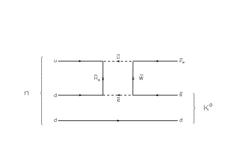
FIG. 1.: A nucleon decay amplitude in SUSY GUTs.

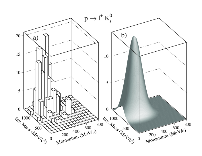
FIG. 2.: a) Simulation for decay mode p $\rightarrow\ell^{+}$K${}^{0}_{s}$, displayed as a lego plot in $M_{inv}$ vs. $\left|\vec{p}_{net}\right|$ space. b) The bi–variate Gaussian surface fitted to the distribution in Fig. 2a.

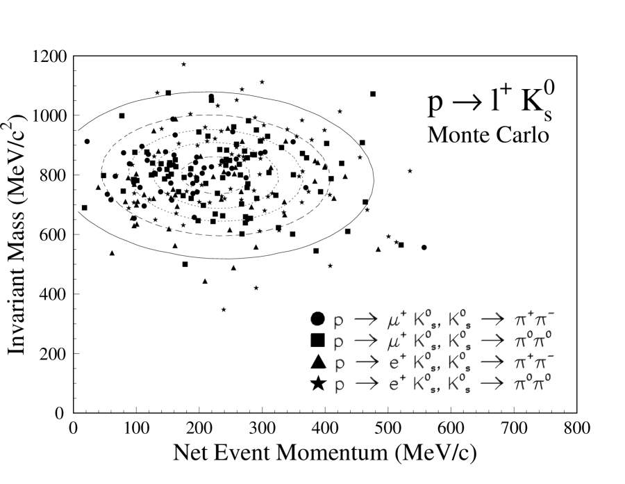
FIG. 3.: The contours of the bi–variate Gaussian surface of Fig. 2 projected onto in the $M_{inv}$ vs. $\left|\vec{p}_{net}\right|$ plane. The region bounded by the outermost contour contains 90% of reconstructed proton decay events and defines the primary kinematic selection used to identify proton decay candidates.

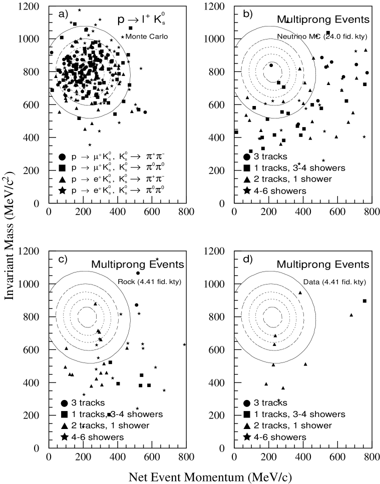
FIG. 4.: For proton decay modes p $\rightarrow\ell^{+}$K${}^{0}_{s}$, the “primary” kinematic selection contour (outermost contour) together with event distributions, in the $M_{inv}$ versus $\left|\vec{p}_{net}\right|$ plane. Distributions show a) the proton decay simulations, b) atmospheric neutrino MC events, c) rock events, and d) data events. The $\mu^{+}$K${}^{0}_{s}$ (e⁺K${}^{0}_{s}$) final states are depicted using solid circles and squares (triangles and stars).

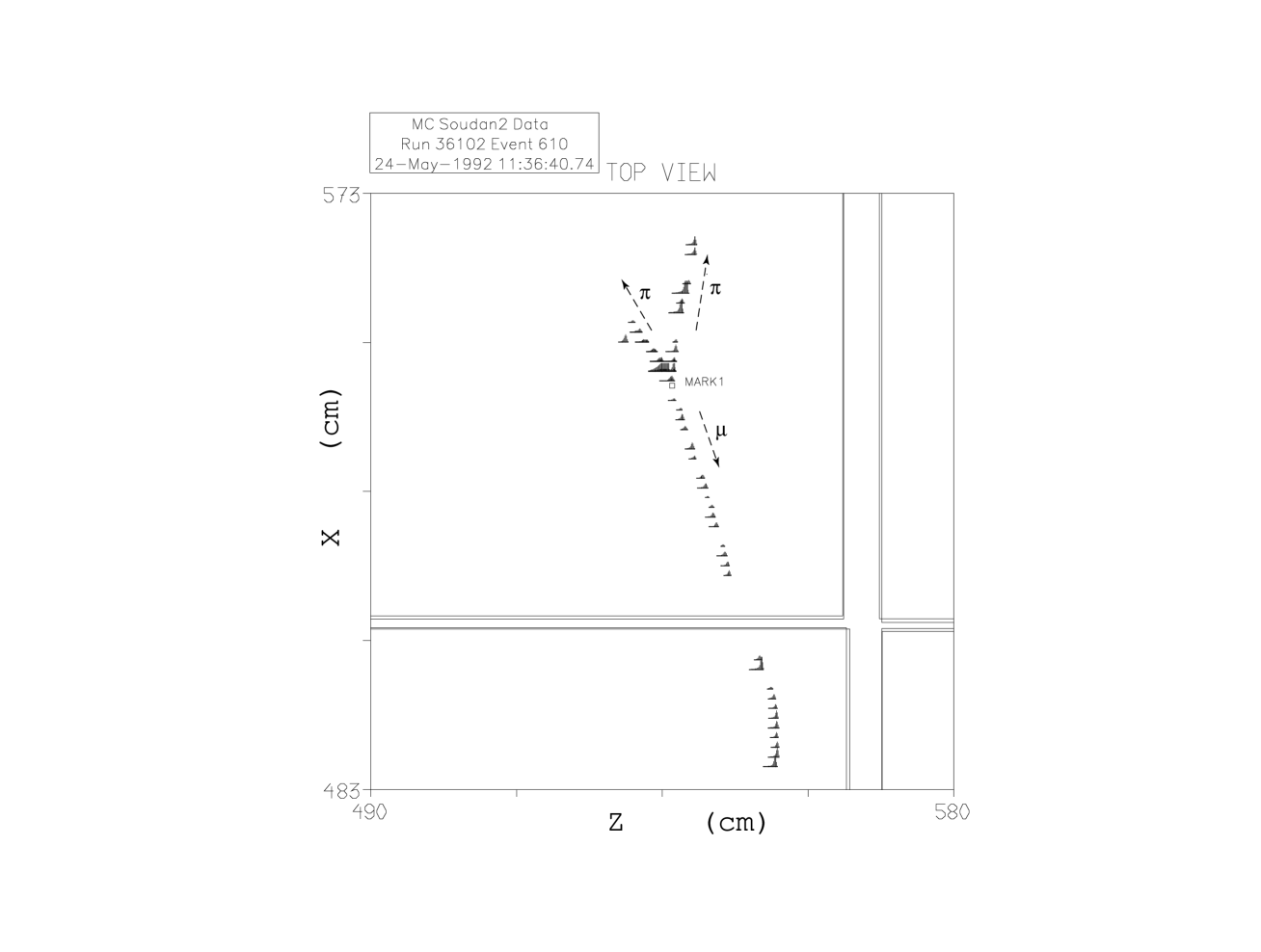
FIG. 5.: Monte Carlo event with full detector response for proton decay p $\rightarrow\mu^{+}$K${}^{0}_{s}$, K${}^{0}_{s}\rightarrow\pi^{+}\pi^{-}$. Here, the anode ($X$) versus drift time ($Z$) projection has been selected from the three scanning views which display anode-time, cathode-time, and anode-cathode images. The open square denoted ‘MARK 1’ depicts the reconstructed primary vertex.

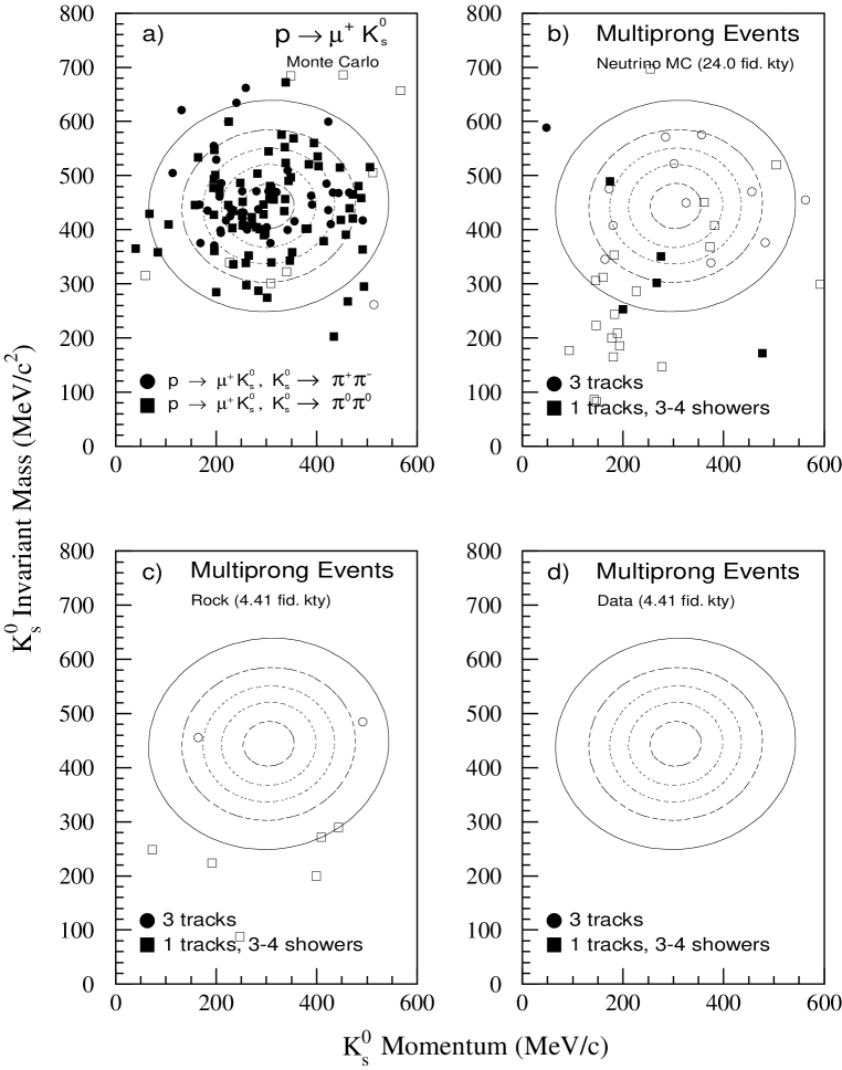
FIG. 6.: For the K${}^{0}_{s}$ subsystem of p $\rightarrow\mu^{+}$K${}^{0}_{s}$ candidates, event distributions plus kinematic selection contour in the plane of $M_{inv}$ versus $\left|\vec{p}_{{\rm K}^{0}}\right|$. Distributions show a) proton decay simulations, b) atmospheric neutrino MC events, c) rock events, and d) data events. Open symbol events fall outside the primary contour of Fig. 4.

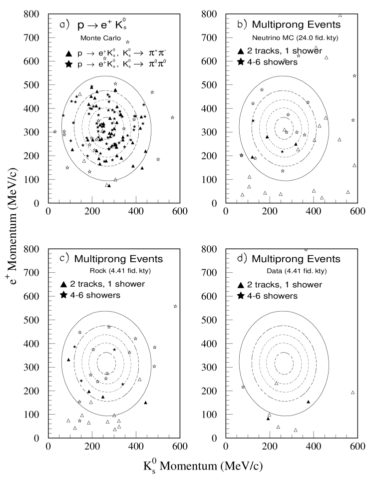
FIG. 7.: The plane of e⁺ momentum versus “K${}^{0}_{s}$” momentum for p $\rightarrow$ e⁺K${}^{0}_{s}$ candidates, showing event distributions plus kinematic selection contours. Distributions show a) proton decay simulations, b) atmospheric neutrino MC events, c) rock events, and d) data events. Open symbols denote events that fall outside of the primary contour and/or the K${}^{0}_{s}$ contour of the K${}^{0}_{s}$ subsystem contour.

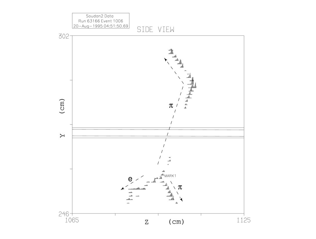
FIG. 8.: Data candidate for proton decay p $\rightarrow$ e⁺K${}^{0}_{s}$, K${}^{0}_{s}\rightarrow\pi^{+}\pi^{-}$, shown in the cathode ($Y$) versus drift time ($Z$) projection.

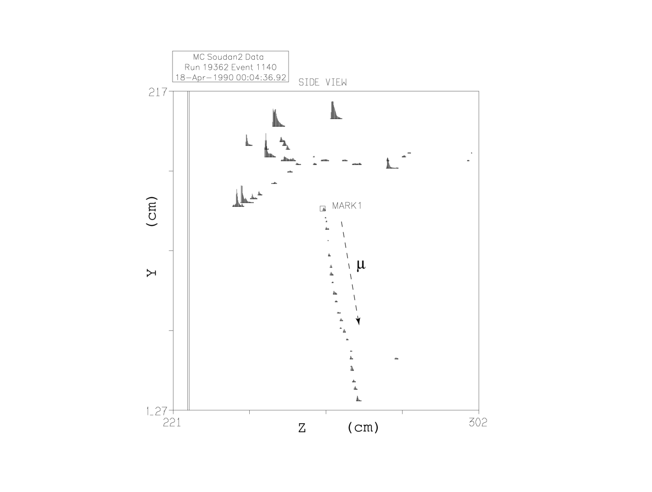
FIG. 9.: Monte Carlo event for p $\rightarrow\mu^{+}$K${}^{0}_{l}$ with subsequent K${}^{0}_{l}$ interaction in the calorimeter medium, shown in the cathode versus drift time projection.

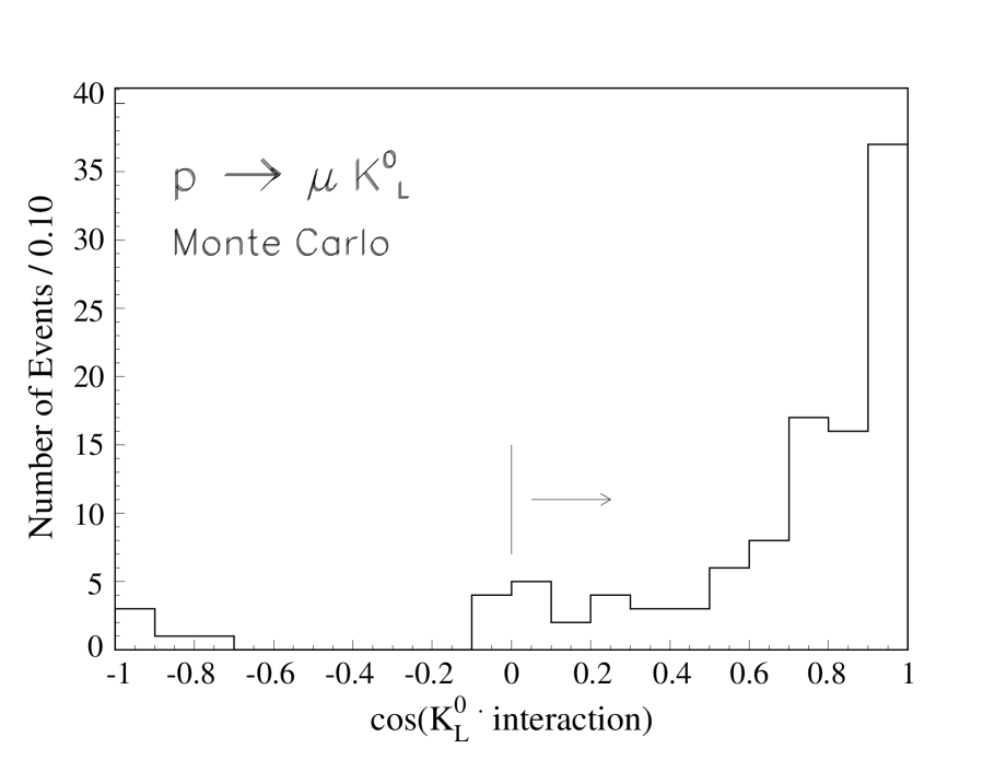
FIG. 10.: Angle between the K${}^{0}_{l}$ flight path and visible net momentum of its subsequent hadronic interaction.

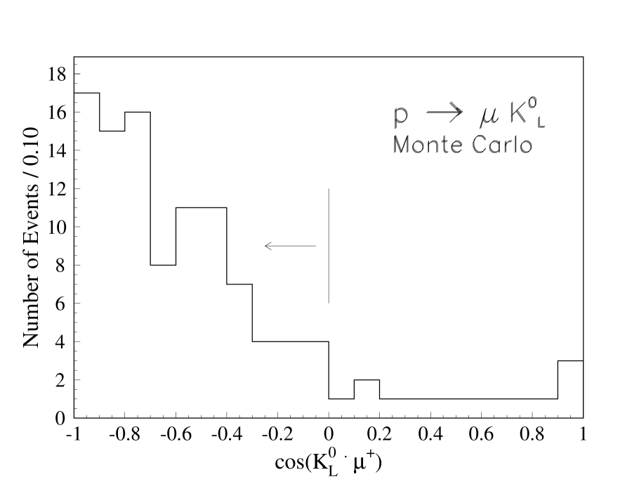
FIG. 11.: Angle between the $\mu^{+}$ track and the K${}^{0}_{l}$ flight path, for p $\rightarrow\mu^{+}$K${}^{0}_{l}$.

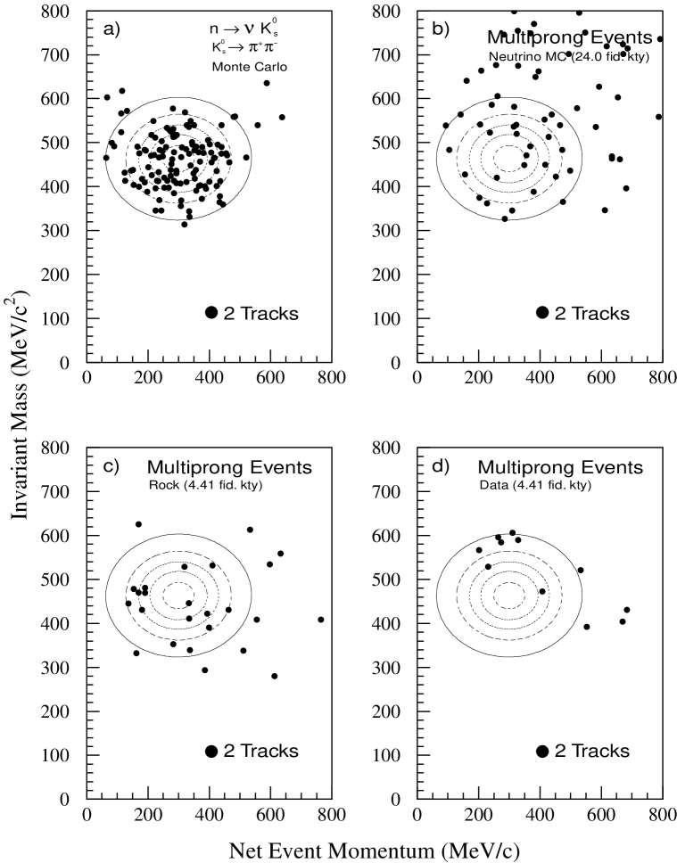
FIG. 12.: For n $\rightarrow\overline{\nu}$K${}^{0}_{s}$, K${}^{0}_{s}\rightarrow\pi^{+}\pi^{-}$, event distributions and kinematic selection contour in the $M_{inv}$ versus $\left|\vec{p}_{net}\right|$ plane. Distributions show a) the neutron decay simulation, b) atmospheric neutrino MC events, c) rock events, and d)the data events. Background events and data candidates having the two–track topology of this mode, are shown via solid circles.

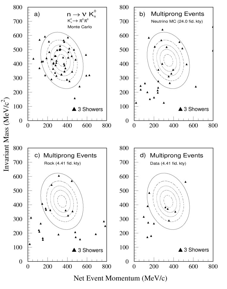
FIG. 13.: For n $\rightarrow\overline{\nu}$K${}^{0}_{s}$, K${}^{0}\rightarrow\pi^{0}\pi^{0}$ yielding three visible showers. Distributions in the $M_{inv}$ versus $\left|\vec{p}_{net}\right|$ plane show three–shower events of a) the neutron decay simulation, b) the atmospheric neutrino MC, c) the rock events, and d) the data events.

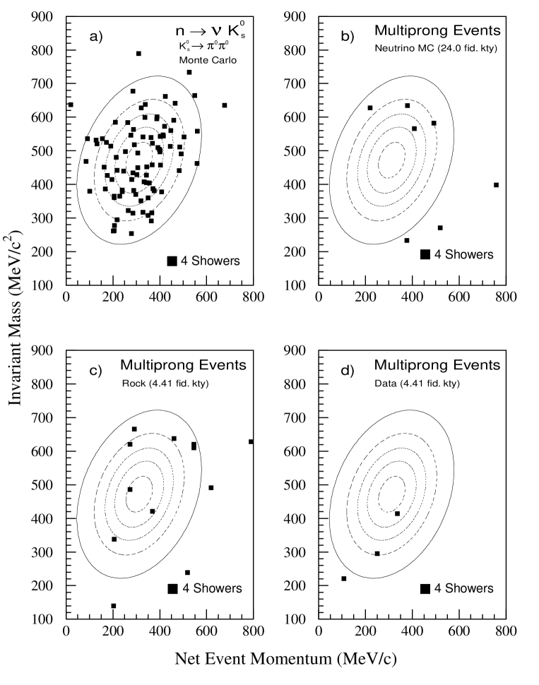
FIG. 14.: For n $\rightarrow\overline{\nu}$K${}^{0}_{s}$, K${}^{0}\rightarrow\pi^{0}\pi^{0}$ yielding four visible showers. Distributions in the $M_{inv}$ versus $\left|\vec{p}_{net}\right|$ plane show four–shower events of a) the neutron decay simulation, b) the atmospheric neutrino MC, c) the rock events, and d) the data events.

REFERENCES

- [1] J. G. Taylor, Prog. Part. Nucl. Phys. 12, 1 (1983).
- [2] G. Kane, in Ann Arbor 1984, Proceedings, TASI Lectures in Elementary Particle Physics 1984, edited by D. N. Williams (TASI Publications, Univ. of Michigan, 1984), pp. 326–363.
- [3] D. V. Nanopoulos, Riv. Nuovo Cim. 8, 1 (1985).
- [4] J. L. Lopez, Rep. Prog. Phys. 58, 819 (1996).
- [5] P. Nath and R. Arnowitt, Phys. Rev. D38, 1479 (1988).
- [6] P. Langacker, in Radiative Corrections, Proceedings of the Tennessee International Symposium on Radiative Corrections: Status and Outlook, edited by B. Ward (World Scientific, Singapore, 1994).
- [7] J. Hisano, H. Murayama, and T. Yanagida, Nucl. Phys. B402, 46 (1993).
- [8] V. Lucas and S. Raby, Phys. Rev. D55, 6986 (1997).
- [9] C. D. Carone et al., Phys. Rev. D53, 6282 (1996).
- [10] K. Babu and S. M. Barr, Phys. Lett. B381, 137 (1996).
- [11] N. Irges, S. Lavignac, and P. Ramond, Phys. Rev. D23, 035003 (1998).
- [12] K.S. Babu, J.C. Pati, and F. Wilczek, Phys. Lett. B423, 337 (1998).
- [13] KGF Collaboration, M.R. Krishnaswamy et al., Phys. Lett. B115, 349 (1982).
- [14] KGF Collaboration, M.R. Krishnaswamy et al., Nuovo Cim. C9, 167 (1986).
- [15] NUSEX Collaboration, G. Battistoni et al., Phys. Lett. B118, 461 (1982).
- [16] Soudan-1 Collaboration, J. Bartlet et al., Phys. Rev. Lett. 50, 651 (1983).
- [17] IMB Collaboration, B. G. Cortez et al., Phys. Rev. Lett. 52, 1092 (1984).
- [18] IMB Collaboration, H. S. Park et al., Phys. Rev. Lett. 54, 22 (1985).
- [19] IMB Collaboration, T.J. Haines et al., Phys. Rev. Lett. 57, 1986 (1986).
- [20] IMB Collaboration, S. Seidel et al., Phys. Rev. Lett. 61, 2522 (1988).
- [21] HPW Collaboration, T.J. Phillips et al., Phys. Lett. B224, 348 (1989).
- [22] IMB-3 Collaboration, C. McGrew et al., Phys. Rev. D59, 052004 (1999).
- [23] Frèjus Collaboration, Ch. Berger et al., Nucl. Phys. B313, 509 (1989).
- [24] Frèjus Collaboration, Ch. Berger et al., Z. Phys. C50, 385 (1991).
- [25] Frèjus Collaboration, Ch. Berger et al., Phys. Lett. B269, 227 (1991).
- [26] Kamiokande Collaboration, K. S. Hirata et al., Phys. Lett. B220, 308 (1989).
- [27] Soudan-2 Collaboration, W. W. M. Allison et al., Phys. Lett. B427, 217 (1998).
- [28] Super-Kamiokande Collaboration, Y. Hayato et al., Phys. Rev. Lett. 83, 1529 (1999).
- [29] Soudan-2 Collaboration, W. W. M. Allison et al., Nucl. Instr. Meth. A376, 36 (1996).
- [30] Soudan-2 Collaboration, W. W. M. Allison et al., Nucl. Instr. Meth. A381, 385 (1996).
- [31] Soudan-2 Collaboration, W.P. Oliver et al., Nucl. Instr. Meth. A276, 371 (1989).
- [32] Soudan-2 Collaboration, W.W.M. Allison et al., Phys. Lett. B391, 491 (1997).
- [33] S.E. Derenzo and R.H. Hildebrand, Nucl. Instr. Meth. 69, 287 (1969).
- [34] T. K. Gaisser, T. Stanev, and G. Barr, Phys. Rev. D38, 85 (1988).
- [35] G. Barr, T.K. Gaisser, T. Stanev, Phys. Rev. D39, 3532 (1989).
- [36] W.A. Mann et al., Phys. Rev. D34, 2545 (1986).
- [37] W. Leeson et al., Soudan 2 internal note PDK–684, 1997 (unpublished).
- [38] A. Bodek and J.L. Ritchie, Phys. Rev. D23, 1070 (1981).
- [39] W.A. Mann et al., Soudan 2 internal note PDK–377, 1988 (unpublished); W. Leeson et al., Soudan 2 internal note PDK–678, 1997 (unpublished).
- [40] R. Merenyi et al., Phys. Rev. D45, 743 (1992); R. Merenyi, Ph.D. thesis, Tufts University, 1990.
- [41] H. Murayama, in Proceedings of the 28th International Conference on High-Energy Physics, edited by Z. Ajduk and A. Wroblewski (World Scientific, Singapore, 1997).
- [42] D. Wall, Ph.D. thesis, Tufts University, 1998.
- [43] C. Garcia-Garcia, Soudan 2 internal note PDK–449, 1990 (unpublished).
- [44] H. R. Gallagher, Ph.D. thesis, University of Minnesota, 1996.
- [45] Soudan-2 Collaboration, W.W.M. Allison et al., Phys. Lett. B449, 137 (1999).
- [46] Super-Kamiokande Collaboration, Y. Fukuda et al., Phys. Lett. B 433, 9 (1998); Phys. Rev. Lett. 81, 1562 (1998); Phys. Lett. B 436, 33 (1998).
- [47] See discussion and references in A. Mann, plenary talk at the XIXth Int. Symposium on Lepton and Photon Interactions at High Energies, Stanford University, Aug. 1999, hep-ex/9912007 (to be published).
- [48] C. Caso et al., Eur. Phys. J. C3, 1 (1998).