Spherical Neutral Detector for VEPP-2M collider

Abstract

The Spherical Neutral Detector (SND) operates at VEPP-2M collider in Novosibirsk studying $e^{+}e^{-}$ annihilation in the energy range up to 1.4 GeV. Detector consists of a fine granulated spherical scintillation calorimeter with 1632 NaI(Tl) crystals, two cylindrical drift chambers with 10 layers of sense wires, and a muon system made of streamer tubes and plastic scintillation counters. The detector design, performance, data acquisition and processing are described.

1 Introduction

For more than 25 years the VEPP-2M $e^{+}e^{-}$ collider has been operating in BINP, Novosibirsk, in the center-of-mass energy range $2E_{0}=0.36\div 1.4$ GeV [1]. Until now its maximum luminosity of $L=3\cdot 10^{30}~{}\mathrm{cm}^{-2}\mathrm{s}^{-1}$ at $E_{0}=510$ MeV was a record for the machines of this class. During this period several generations of detectors performed experiments at VEPP-2M. Much of the current data on particles properties [2] at low energy region were obtained in these experiments.

The SND detector is an advanced version of its predecessor – the Neutral Detector (ND) [3, 4], which completed its five-year experimental program in 1987 [5]. The SND detector [6] operates at VEPP-2M since 1995 [7, 8, 9, 10]. Its main part is a three-layer spherical calorimeter consisting of 1632 crystals NaI(Tl). The SND is a general purpose detector optimized for multi-photon final states.

2 General overview

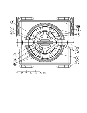
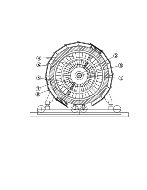
Figure 1: SND detector, section along the beams: (1) beam pipe, (2) drift chambers, (3) scintillation counter, (4) light guides, (5) PMTs, (6) NaI(Tl) crystals, (7) vacuum phototriodes, (8) iron absorber, (9) streamer tubes, (10) 1 cm iron plates, (11) scintillation counters, (12) and (13) elements of collider magnetic system.

Figure 2: SND detector, section across the beams: (1) beam pipe, (2) drift chambers, (3) scintillation counter, (4) NaI(Tl) crystals, (5) vacuum phototriodes, (6) iron absorber, (7) streamer tubes, (8) scintillation system.

The detector layout is shown in Figs. 2, 2. Electron and positron beams collide inside the beryllium beam pipe with a diameter of 2 cm and 1 mm wall. The beam pipe is surrounded by tracking system consisting of two drift chambers and a cylindrical scintillation counter between them. The solid angle coverage of the tracking system is about $98\%$ of $4\pi$.

The three-layer spherical electromagnetic calorimeter based on NaI(Tl) crystals surrounds the tracking system. The total calorimeter thickness for particles originating from the interaction region is 34.7 cm (13.4 $X_{0}$) of NaI(Tl) and the total solid angle is $90\%$ of $4\pi$.

Outside the calorimeter a 12 cm thick iron absorber is placed in order to attenuate the residuals of electromagnetic showers. It is surrounded by segmented muon system which provides both muon identification and cosmic background suppression . Each segment consists of two layers of streamer tubes and a plastic scintillation counter, separated from the tubes by 1 cm iron plate. The iron layer between the tubes and the counter reduces the probability of their simultaneous firing by photons produced in $e^{+}e^{-}$ collisions to less than $1\%$ for 700 MeV photons.

3 Calorimeter

3.1 Calorimeter layout

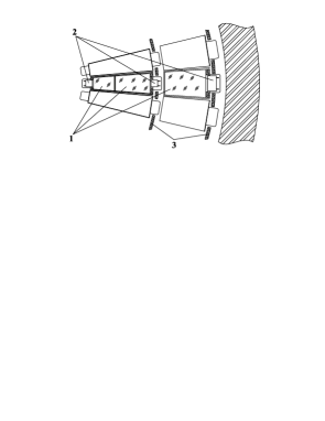
Figure 3: NaI(Tl) crystals layout inside the calorimeter: (1) NaI(Tl) crystals, (2) vacuum phototriodes, (3) aluminum supporting hemispheres.

Figure 4: Electronics channel of the SND calorimeter: (NaI) NaI(Tl) scintillator, (VPT) vacuum phototriode, (CSA) charge-sensitive preamplifier, (ADC) analog to digital converter, (Gen) calibration generator, (SHA) shaping amplifier, (ATT) computer-controlled attenuator, (FLT) first-level trigger

Spherical shape of the SND calorimeter provides relative uniformity of response over the whole solid angle. Pairs of counters of the two inner layers with thickness of 2.9 and 4.8 $X_{0}$ ($X_{0}=2.6$ cm) are sealed in thin (0.1 mm) aluminum containers, fixed to an aluminum supporting hemisphere (Fig. 4). Behind it, the third layer of NaI(Tl) crystals, 5.7 $X_{0}$ thick, is placed. The gap between the adjacent crystals of one layer is about 0.5 mm. The total number of counters is 1632, the number of crystals per layer varies from 520 to 560. The total mass of NaI(Tl) is 3.5 t.

The polar angle coverage of the calorimeter is $18^{\circ}\leq\theta\leq 162^{\circ}$. The calorimeter is divided into two parts: “large” angles $36^{\circ}\leq\theta\leq 144^{\circ}$ and “small” angles — the rest. The angular dimensions of crystals are $\Delta\phi=\Delta\theta=9^{\circ}$ at “large” angles and $\Delta\phi=18^{\circ},\Delta\theta=9^{\circ}$ at “small” angles. Each layer of the calorimeter consists of crystals of eight different shapes.

The crystal widths approximately match the transverse size of an electromagnetic shower in NaI(Tl). Two showers can be distinguished if the angle between them is larger than $9^{\circ}$. If this angle exceeds $18^{\circ}$ the energies of the showers can be measured with the same accuracy as for isolated shower. A high granularity of the calorimeter is especially useful for the detection of multi-particle events. For example, the detection efficiency for 7-photon events of the process $\phi\to\eta\gamma$, $\eta\to 3\pi^{0}$ is close to $15\%$.

The light collection efficiency varies from $7\%$ to $15\%$ for crystals of different calorimeter layers. The scintillation light signals from the crystals are detected by vacuum phototriodes [11] with a photocathode diameter of 17 mm in the first two layers and 42 mm in the third layer. The average photocathode quantum efficiency is about $15\%$ and the mean tube gain is about 10.

The electronics of the calorimeter (Fig. 4) consists of

1. the charge sensitive preamplifiers (CSA) with a conversion coefficient of 0.7 V/pC,

2. 12-channel shaping amplifiers (SHA) with a remote controlled gain that can be set to any value in the range from 0 to a maximum with a resolution of 1/255.

3. 24-channel 12-bit analog to digital converter (ADC) with a maximum input signal $U_{\mathrm{max}}=2\mathrm{V}$,

Each calorimeter channel can be tested using a precision computer-controlled calibration generator. The amplitude of its signal can be set to any value from 0 to 1 V with a resolution of 1/4096. The equivalent electronics noise of individual calorimeter channel lies within the range of $150\div 350$ keV.

To produce signals for the first-level trigger the SHAs are collected into 160 modules corresponding to 160 towers (4 crystals from three layers located one under another). The towers divide calorimeter into 20 sectors of $18^{\circ}$ in azimuthal direction and into 8 rings of $18^{\circ}$ in polar direction.

3.2 Energy calibration

Calorimeter is calibrated using cosmic muons [12] and $e^{+}e^{-}\rightarrow e^{+}e^{-}$ process events [13]. A fast preliminary calibration based on cosmic muons gives the constants for calculation of energy deposition in the calorimeter crystals. These constants are used for levelling responses of all crystals in order to obtain an uniform first-level trigger energy threshold over the whole calorimeter and represent seed values for the more precise calibration procedure, using $e^{+}e^{-}\rightarrow e^{+}e^{-}$ events. The cosmic calibration procedure is based on the comparison of the experimental and simulated energy depositions in the calorimeter crystals for cosmic muons. The detailed description of the method is given in [12]. The statistical accuracy of $1\%$ in the calibration coefficients was achieved. After cosmic calibration the peak positions in the measured energy spectra for photons and electrons agree at a level of about $1\%$ with the actual particle energies (Fig. 6).

The cosmic calibration procedure performed weekly, between the experimental runs takes less than 5 hours. For a one-week period between consecutive calibrations the coefficients stability was better than $1.5\%$. Changes in the conversion constants were also monitored daily, using the calibration generator. They could either drift slowly with electronics gain changes or show large leaps due to replacement of broken electronics modules.

To achieve highest possible energy resolution, the precise OFF-LINE calibration procedure, based on analysis of $e^{+}e^{-}\rightarrow e^{+}e^{-}$ events, was implemented. The calibration coefficients are obtained by the minimization of the r.m.s. of the total energy deposition spectrum for the electrons with fixed energy. The detailed description of the procedure is given in [13]. To obtain the statistical accuracy of about $2\%$ the sample of at least 150 electrons per crystal is needed. SND acquires such a sample daily when VEPP-2M operates in the center-of-mass energy $2E_{0}\sim 1$ GeV. The average difference in calibration coefficients obtained using cosmic and $e^{+}e^{-}$ calibration procedures is about $4\%$, while the $e^{+}e^{-}$ calibration improves the energy by $10\%$. For example, the energy resolution for 500 MeV photons improves from $5.5\%$ to $5\%$.

3.3 Energy and angular resolution

The calorimeter energy resolution is determined mainly by the fluctuations of the energy losses in the passive material before ($0.17X_{0}$) and inside ($0.17X_{0}$) the calorimeter and leakage of shower energy through the calorimeter. The most probable value of the energy deposition for photons in the calorimeter is about $93\%$ of their energy (Fig. 6).

In order to compensate for the shower energy losses in passive material and improve energy resolution the photon energy is calculated as:

$$E=\alpha_{1}\cdot E_{1}+\alpha_{2}\cdot E_{2}+\alpha_{3}\cdot E_{3},$$ (1)

where $E_{1}$ is energy deposition in the first and second layers of the central tower of the shower, $E_{2}$ is energy deposition in the first two layers outside the central tower, $E_{3}$ is energy deposition in the third layer, $\alpha_{i}$ are energy dependent coefficients. Here the tower is the three counters of the 1, 2 and 3 layers with the same $\theta$ and $\phi$ coordinates and the central tower corresponds to the shower center of gravity.

The $\alpha_{i}$ coefficients were determined from simulation of photons with energies from 50 to 700 MeV. For each photon energy the objective function:

$$M=\sum\limits_{k}(E^{*}-E_{k})^{2},$$ (2)

was minimized over $\alpha_{i}$. Here $E^{*}$ is a known photon energy, $E_{k}$ is the energy calculated using expression (1), $k$ is a photon number. The energy dependences of $\alpha_{i}$ were approximated by the smooth curves. The approximation was done separately for the showers starting in different layers. As a result the calorimeter resolution was improved by $10\%$.

The apparatus effects, such as nonuniformity of light collection efficiency over the crystal volume and electronics instability also affect energy resolution:

$$\sigma_{E}/E(\%)=\sigma_{1}(E)\oplus\sigma_{2}(E)\oplus\sigma_{3}(E),$$ (3)

where $\sigma_{1}(E)$ is the energy resolution obtained using Monte Carlo simulation without effects mentioned above, $\sigma_{2}(E)$ is electronics instability and calibration accuracy contribution, $\sigma_{3}(E)$ is the contribution of nonuniformity of light collection over the crystal volume. For example, for 500 MeV photons $\sigma_{E}/E=5\%$, $\sigma_{1}(E)=3\%$, $\sigma_{2}(E)=1.2\%$ and $\sigma_{3}(E)=3.8\%$. The dependence of the calorimeter energy resolution on photon energy (Fig. 8) can be approximated as:

$$\sigma_{E}/E(\%)={4.2\%\over\sqrt[4]{E(\mathrm{GeV})}}.$$ (4)

The distribution function of energy deposition in the SND calorimeter outside the cone with the angle $\theta$ around the shower direction was obtained using Monte Carlo simulation:

$$E(\theta)=\alpha\cdot exp(-~{}\sqrt[]{\theta/\beta}),$$ (5)

It turned out that $\alpha$ and $\beta$ parameters are practically independent of photon energy in a wide energy range $50\div 700$ MeV. The method of estimation of photon angles based on this dependence was introduced in [14]. The dependence of the angular resolution on the photon energy shown in Fig. 8 can be approximated as:

$$\sigma_{\phi}={0.82^{\circ}\over\sqrt[]{E(\mathrm{GeV})}}\oplus 0.63^{\circ}.$$ (6)

The two-photon invariant mass distributions in $\phi\rightarrow\eta\gamma$ and $\phi\rightarrow\pi^{+}\pi^{-}\pi^{0}$ events (Figs. 10, 10), show clear peaks at $\pi^{0}$ and $\eta$ mesons masses. Invariant mass resolution is equal to 11 MeV for $\pi^{0}$ and 25 MeV for $\eta$. The kinematic fitting [15] improving angular and energy resolution of the detector. For example for $\phi\rightarrow\eta\gamma,\pi^{0}\gamma$ decays kinematic fit improves two-photon invariant mass resolution by a factor of 1.5 (Fig. 12).

3.4 Particle identification

The discrimination between electromagnetic and hadronic showers in the calorimeter is usually based on difference in total energy deposition (Fig. 12). Multilayer structure of the SND calorimeter provides additional means of particle identification based on differences in longitudinal energy deposition profiles. The distributions of energy deposition over layers for $e^{\pm}$ and $\pi^{\pm}$ is shown in Fig. 13. Two areas of pions concentration in this scatter plot correspond to nuclear interaction of pions and pure ionization losses in the first two layers of NaI(Tl). Utilizing differences in energy depositions for electrons and pions the special discrimination parameter was constructed. In the $\rho(770)$ energy region it provides $99\%$ selection efficiency for $e^{+}e^{-}\rightarrow\pi^{+}\pi^{-}$, keeping contamination by $e^{+}e^{-}\rightarrow e^{+}e^{-}$ events $\sim 1\%$

The distribution of energy depositions in the calorimeter layers is also used for $K_{L}$ identification, for example in $\phi\rightarrow K_{S}K_{L}$ decays, making feasible studies of rare $K_{S}$ decays.

The $e/\pi$ and $\gamma/K_{L}$ separation parameters based on the differences in energy deposition profiles in transverse direction were also constructed. Their detailed description is given in [16].

4 Tracking system

4.1 Tracking system layout

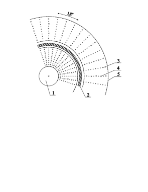
Figure 14: SND coordinate system view across the beams: (1) beam pipe, (2) scintillation counter, (3) field shaping wires, (4) anode wires, (5) field shaping strips

The tracking system (Fig. 14) consists of two cylindrical drift chambers and a cylindrical plastic scintillation counter (CSC)[17] between them.

The counter length, inner diameter and thickness are 37, 12.6 and 0.5 cm respectively. In azimuth direction it is divided into 5 segments. The counter has a wavelength shifter fiber readout. It provides the time synchronization with beams collisions and produces signals for the first-level trigger. The time resolution of the counter is about 1.4 ns.

The inner (“long”) drift chamber (LDC) has the length of 40 cm, outer and inner diameters of 4 and 12 cm respectively. The corresponding dimensions of the outer (“short”) drift chamber (SDC) are 25, 14 and 24 cm.

Both chambers consist of 20 jet-type drift cells. Each cell has 5 gold-plated tungsten sense wires with a diameter of 20 $\mu$m. A $\pm 300$ $\mu$m staggering of the sense wires in azimuth direction resolves the left/right ambiguity. Field wires are made of bronze-coated titanium with a diameter of 100 $\mu$m. The total numbers of sense and field wires in each chamber are 100 and 260 respectively. The drift chambers flanges are made of fiberglass with a thickness of 10 mm. The wires are fixed using copper pins, precisely positioned in the flanges. The cylindrical fiberglass walls of both chambers have three layers of copper electrodes: field strips, parallel to the wires, and sense (cathode) strips, transverse to the wires, with electrodes for signal output. The effective thickness of tracking system is about $0.1X_{0}$. Both chambers operate with a $90\%\mathrm{Ar}+10\%\mathrm{CO}_{2}$ gas mixture.

The circuitry of the electronics channel of the tracking system is shown in Fig. 15. The field wires and strips operate at different potentials in the range of 1–3 kV to provide the uniform drift field. The sense wires operating at ground potential are DC coupled to preamplifiers, while for cathode strips capacitive AC coupling is used. The amplified analog signals from each sense wire are transmitted to the amplitude- and time-to-digital converters (ADC and TDC). So, two amplitudes from both ends and a common timing are measured for each wire.

4.2 Calibration of the tracking system

The calibration of the tracking system consists of several procedures to obtain the coefficients for conversion of measured times and amplitudes into the track coordinates and specific ionization losses ($dE/dx$).

The sense wires are calibrated electronically using the generator. The generator signals with varying amplitudes are switched between the preamplifiers on both ends of the wires. For each generator amplitude an average ADC count is calculated. These data provide calibration constants for $z$-coordinate measurement by means of charge division method:

$$z=l_{0}\cdot{{B_{L}Q_{L}-B_{R}Q_{R}}\over{Q_{L}+Q_{R}}}.$$ (7)

$Q_{L(R)}=A_{L(R)}U_{L(R)}$ is the charge collected at the left (right) end of the wire, $U_{L(R)}$ is the measured amplitude in ADC counts, $A_{L(R)}$ is the coefficient for conversion of the amplitude in ADC counts into units of electric charge, $B_{L(R)}$ is a conversion coefficient from charge into a normalized coordinate, $l_{0}$ is the wire length.

The $z$-coordinate is also measured by means of cathode strip readout. To obtain a conversion coefficients from the ADC counts into the input signal amplitudes, the electronics channels are calibrated using generator. The track coordinate can be calculated then as:

$$z=Z_{a}+\Delta Z,$$ (8)

where $Z_{a}$ is the coordinate of the strip with the maximum amplitude (central strip), $\Delta Z$ is the correction obtained from the ratio of the amplitudes at all fired strips to the amplitude at the central strip. $\Delta Z=f(q_{a-1},q_{a},q_{a+1})$, where $a$ is the central strip number. Function $f$ was obtained using experimental cosmic muon sample, under assumption of their uniform distribution in $z$.

The small differences in wire lengths $z$-coordinates of their centers contribute to the accuracy of $z$-coordinate measurements by charge division. To eliminate this contribution a calibration procedure based on analysis of $e^{+}e^{-}\rightarrow e^{+}e^{-}$ events was performed. Cathode strips hit by one track were fitted and correction coefficients for each wire obtained. The corrected $z$-coordinate reads:

$$z=z_{w}\cdot(1+\Delta L/L)-\Delta z_{0},$$ (9)

where $z_{w}$ is the track coordinate measured by charge division, $\Delta L/L$ is the corresponding wire length correction, $\Delta z_{0}$ is the longitudinal bias of the wire with respect to the center of the tracking system.

Due to absorption in the gas mixture the average signal amplitude on a wire decreases by 1.5 times per 1 cm of the drift distance. The dependence of the average amplitude on drift distance can be approximated as:

$$A(R)=A_{0}(1-R/l),$$ (10)

where $R$ is a measured drift distance. Attenuation length $l$ is obtained using $e^{+}e^{-}\rightarrow e^{+}e^{-}$ events and $A_{0}$ is the calibration constant.

For the conversion of the drift time into the distance $R(T)$ from track to the wire the $r-\phi$ calibration based on uniformity of $\phi$ distribution of $e^{+}e^{-}\to e^{+}e^{-}$ events was performed.

4.3 Drift chambers efficiency and resolution

The efficiency of wires and cathode strips at low counting rates is close to $100\%$. The drift chambers total counting rate is about 150 kHz for the beam currents $I_{e^{+}}=I_{e^{-}}\sim 50$ mA and luminosity of $\sim 2\cdot 10^{30}$ $\mathrm{cm}^{-2}\mathrm{s}^{-1}$. The pile up hits degrade accuracy of coordinates measurements. In order to increase the accuracy the hits distant from the track, are removed from the fit. Thus the final wire efficiency in track reconstruction is about $95\%$. The accuracies of coordinate measurements by drift times and charge division methods is about 180 $\mu$m and 3.6 mm respectively.

The tracking system angular resolution was measured using distributions in $\Delta\theta$ and $\Delta\phi$ acollinearity angles between tracks in the $e^{+}e^{-}\rightarrow e^{+}e^{-}$ and $e^{+}e^{-}\rightarrow\pi^{+}\pi^{-}$ events as $\sigma_{\theta}=\sigma_{\Delta\theta}/\sqrt{2}$ and $\sigma_{\phi}=\sigma_{\Delta\phi}/\sqrt{2}$, where $\sigma$ is by definition the full width of the distribution at half-maximum divided by 2.36.

The polar angle resolution $\sigma_{\theta}$ depends on the accuracy of $z$-coordinate measurement. The use of cathode strips together with sense wires provides 1.5 times improvement of the resolution relatively to charge division only. Finally, $\sigma_{\theta}=1.7^{\circ}$ for electrons and $\sigma_{\theta}=1.9^{\circ}$ for pions. The azimuth angle resolution $\sigma_{\phi}=0.51^{\circ}$ for electrons (Fig. 16) and $\sigma_{\phi}=0.54^{\circ}$ for pions. The impact parameter in $r-\phi$ plane resolution $\sigma_{R}=0.5$ mm. Small differences in angular resolutions for electrons and pions can be attributed to the different average ionization losses and $\theta$ distributions for these particles.

The achieved $dE/dx$ resolution is about $30\%$ and it is not sufficient for $e/\pi$ separation, but $\pi^{\pm}/K^{\pm}$ separation in the energy region of $\phi$-meson production is possible (Fig. 18).

5 Muon system

The muon system provides suppression of cosmic background and identification of the muons produced in the beams collisions at energies above 450 MeV.

5.1 Muon system layout

The muon system (Figs. 2, 2) consists of 16 ($200\times 40\times 1$ $\mathrm{cm}^{3}$) scintillation counters and two layers of streamer tubes. Each counter consists of two sheets of plastics scintillator glued together. Light is collected from two sides of the scintillator via the acrylic light guides to the pair of PM tubes with photocathode diameter of 40mm. Each counter is wrapped in aluminized mylar and put in a thin steel container.

The barrel part of the streamer tubes system consists of 14 modules with 40 cm width, two end-cap modules have the width of 80 cm. The module length is 2 m. Each module consists of 16 tubes arranged in two layers. The tubes are made of 300 $\mu$m stainless steel and have a diameter of 4 cm. Along the tube axis a 100 $\mu$m gold-plated molybdenum wire is strung. Streamer tubes are filled with a $75\%\mathrm{Ar}+25\%n$-pentane gas mixture, which provides operation in a streamer mode at wire potential $\sim 4000$ V.

The electronics channel of the muon system [18] is shown in Fig. 18. The analog signals from PMTs are carried to the discriminators where the amplitude and timing signals are formed, and then transmitted to ADC and TDC. The signals from opposite ends of the streamer tubes are applied to the time expander, where the signal with a duration proportional to their time difference is formed for further digitization by TDC. The signals from the tubes and counters are also used in the first-level trigger.

5.2 Muon system calibration

$Z$-coordinate of the particle track is obtained using the time difference between the signals from the opposite ends of streamer tubes :

$$Z={l\over 2}-l\cdot{{C-\Delta T}\over C},$$ (11)

where $l$ is the wire effective length, known with the accuracy of about $2\%$, $\Delta T$ is the time difference between the signals from wire ends expressed in TDC counts, $C$ is the calibration coefficient, obtained using $\Delta T$ distribution for cosmic muons. Stability of the electronics was checked daily using calibration generator.

To obtain the time of scintillation counter hit the following expression is used:

$$t=K\cdot T+\Delta t,$$ (12)

where $T$ is a TDC count, $K$ is a coefficient for TDC count to time conversion, obtained from cosmic muons spectrum, $\Delta t$ is a correction accounting for differences in the individual cables lengths and PM tubes delay times. $\Delta t$ is obtained as the time difference between the hits in muon scintillation counter and tracking system scintillation counter, using $e^{+}e^{-}\rightarrow\mu^{+}\mu^{-}$ events and cosmic muons. Cosmic muons are also used for the energy calibration of the scintillation counters (average energy losses are $2$ MeV/cm). The energy deposition in the counter $E=k\cdot U$, where $U$ is the signal amplitude in ADC counts, $k$ is the coefficient of conversion from ADC counts to the units of MeV. To consider the amplitude dependence on the $Z$-coordinate of the muon track due to the light absorption in scintillator the muon track is fitted using streamer tubes.

5.3 Efficiency and time resolution of the muon system

The muon system veto signal provide the 50 times cosmic background suppression in actual experimental conditions.

A longitudinal coordinate of the track is obtained from the tube number. If only one tube is fired, then resolution $\sigma=d/\sqrt{12}=1.2$ cm, where $d=4$ cm is the tube diameter. When the tubes in both layers are hit the resolution is $\sigma=0.6$ cm determined by the shift between layers. The $Z$-coordinate resolution $\sigma_{Z}=3.3$ cm.

To obtain the time of scintillation counters hit with respect to beams crossing, special corrections for light propagation time were applied. The corrections take into account the effective velocity of light in the scintillator ($\sim 15$ ns/cm) and dependence of the counter firing time on the signal amplitude due to fixed discriminator threshold. After corrections the time resolution of the counters is 1 ns (Fig. 20).

6 Data acquisition system

6.1 Electronics

The SND data acquisition system (DAQ) [19] (Fig. 20), based on KLUKVA electronics standard [20] developed at BINP.

Analog signals from the detector elements come to the front-end electronics located on SND systems. Then the signals are carried via screened twisted pairs to digitizing electronics (ADCs and TDCs). The signals from the calorimeter and cathode strips are shaped by shaping amplifiers before digitization. The digitizers and shapers reside in KLUKVA crates. One crate holds 16 data conversion modules, one first-level trigger (FLT) interface module (IFLT) and readout processor module (RP). The data conversion modules provide data, which are transferred via KLUKVA crate bus to IFLT modules for further use in FLT.

Two types of digitizers are used: TDCs with“common stop” and ADCs with “common start”. The first type [21] provides the drift time measurement. Signals from sense wires start 250 MHz counters and FLT signal stops drift time digitizing. If FLT signal does not arrive within 1 $\mu$s the counters reset. The second type [22] is used for digitization of signals from the calorimeter and DC cathode strips. The digitization starts by FLT signal and lasts 80 $\mu$s. The digitizers (about 3000 channels) occupy 13 KLUKVA crates.

After the digitization the data are extracted from the ADC and TDC modules by the RP in 100 ns. An RP memory contains the pedestals of all channels placed in the crate. RP compares the data with pedestals and performs zeros suppression. As a result average event size decreases down to about 1kB. The RP internal memory keeps digitized data for two events, providing with the internal registers of ADCs and TDCs 3-level derandomizing of data flow. The time needed for event digitization and processing is about 200 $\mu$s. The data from RP are transmitted to the ON-LINE computer via special CAMAC modules [20].

6.2 First-level trigger

The fast analog signals of energy deposition in calorimeter towers and logical signals from wire hits in drift chambers are collected by IFLT modules. The IFLTs and analog and logical summation modules form the signals for specialized trigger modules: Calorimeter Logic, Track Logic, Layers Logic, and Energy Thresholds, producing 48 different FLT components (Fig. 21). The input information for Calorimeter Logic [23] is 20 signals from sectors and 8 signals from rings, produced by the logical summation of the hit towers with the energy deposition higher than 25 MeV. The sectors signals go to the address bus of 1MB static RAM, where the look-up table is stored. The information from rings from another 32 kB RAM is added. So, according to the RAM contents, the components of the FLT depending on the number of hit towers and their relative positions are produced. FLT components can be easily changed by RAM reprogramming.

The Energy Thresholds module contains 10 discriminators with programmable threshold. As an input information the analog signals of total energy deposition and energy deposition at “large” angles are used.

A Track Logic [24] is constructed using the programmable logic devices. As the input information the following logical signals are used: 100 signal lines from LDC wires, 20 signals from the first two layers of SDC and 20 signals from the calorimeter sectors. Hit wires patterns in LDC corresponding to tracks from interaction point are looked for. Then the track continuation in SDC and calorimeter is checked. Resulting signals contain information on the number of found tracks and their relative positions. The Layer Logic is based on static RAM and as input data uses 10 logical OR signals from LDC and SDC layers. It produces three components, each being the various combination of input signals, according to the RAM contents.

The FLT logic is implemented as a pipeline working at 16 MHz clock rate, which is the collider beam circulation frequency. Such FLT organization provides zero “dead” time, while the FLT decision latency is about 800 ns.

The main source of background are electromagnetic showers produced in the collider magnets and lenses by stray particles from the beam. The FLT background suppression is based on the following differences in the properties of physical and background events:

1. the total energy deposition in the calorimeter for physical events is larger than for background events;

2. hits in physical events form two or more compact clusters in the calorimeter;

3. particles in physical events originate from the collider interaction region;

4. in the background events the main part of the total energy deposition in the calorimeter is localized at “small” angles.

The most often used FLT components are:

1. “OR” of all calorimeter towers used as a master signal for FLT Mask Modules with a time resolution better than 5 ns, while the time between collisions is 60 ns;

2. two well separated towers hit;

3. two collinear towers hit;

4. hit tower at an angle larger than $54^{\circ}$ with respect to the beam;

5. two hit towers with azimuth angle between them larger than $90$ degrees;

6. the total energy deposition and the energy deposition at “large” angle is larger than certain threshold;

7. LDC track, LDC track continued in SDC, and LDC track continued in SDC and calorimeter;

8. two separate tracks in LDC;

9. the muon system veto.

Final FLT decision is produced by 10 Mask Modules, each taking 48 FLT components as inputs. It is possible to define 10 different trigger types by writing appropriate masks into the Mask Modules. Four trigger types select events containing charged particles (“charged” triggers), other four select events with neutral particles only (“neutral” triggers), one trigger selects cosmic muons for muon system calibration and the last selects the $e^{+}e^{-}\rightarrow e^{+}e^{-}$ events for on-line luminosity measurement. For all “neutral” triggers the muon system veto is enabled.

In average experimental conditions the calorimeter and drift chambers counting rates are about 80 kHz and 150 kHz respectively. The FLT reduces the trigger rate to a level of $\sim 80$ Hz.

6.3 Data Taking

Data from RP RAMs are read into the VAXserver 3300 computer via the CAMAC interface modules at a rate of 2 ms/event. The computer RAM is used for data flow derandomization. Then the data are transmitted to the VAXstation-4000/60 workstation, where events are packed in a special SND format [26]. For packed events the partial reconstruction (see section 7) is performed. The reconstructed events are processed by the software 3-rd level trigger which suppresses beam background and cosmic events, decreasing the event rate by a factor of 2. In addition it counts $e^{+}e^{-}\rightarrow e^{+}e^{-}$ and $\gamma\gamma$ events for on-line luminosity monitoring. The total time required for partial reconstruction and 3-rd level trigger decision is $\sim 10$ ms/event. Average DAQ dead time is about $10\%$.

Events selected by the software trigger are written on file on the local disk. After each experimental run files are automatically saved to 4 GB tapes by the data management system ART [19, 27].

During the run several concurrent processes collect information about detector subsystems, DAQ, and collider performance. Real-time access to these data is provided by information management system IMAN [28]. The special process monitors this information and rises alarm if hardware or software problems are detected.

Stability of SND subsystems is monitored using precision generator signals to test all electronics channels. This procedure takes about 20 minutes and is performed daily.

7 Data processing

Large volume of data collected during experimental runs requires quick and adaptable processing. The data processing is based on CERN software such as HBOOK [30], HIGZ [31], PAW [32], MINUIT [33], as well as programs developed in BINP:

1. GIST [29] provides common environment for data processing, user interface with other codes, data storage in format compatible with HBOOK package for further analysis using PAW;

2. COCHA [26] provides the data input/output and storage. The data representation is based on entity – relationship model;

3. event reconstruction code;

4. code for events visualization based on HIGZ graphics package;

5. ART [27] provides transparent access to data stored on tapes and disks.

Processing of experimental data consists of several steps:

1. SND subsystems are calibrated using $e^{+}e^{-}\rightarrow e^{+}e^{-}$ and $\mu^{+}\mu^{-}$ events;

2. events are reconstructed and parameters of particles are calculated; according to these parameters the events divided into $\sim 20$ different physical classes;

3. for each experimental run the $e^{+}e^{-}\rightarrow e^{+}e^{-}$ and $\gamma\gamma$ events are counted for the integrated luminosity determination, efficiencies of SND systems are obtained; collected information about SND and collider performance is used in the analysis, for example, to determine the beam energy more precisely;

4. the selected events are used for the physical analysis.

Event reconstruction is performed in a following sequence. First step is a search for separated clusters in the calorimeter. Then the track reconstruction in drift chambers is performed. Tracks are linked to the calorimeter clusters. The clusters with energy depositions of more than 20 MeV not linked to tracks in DC are considered as photons. For charged tracks no requirements on energy depositions in the calorimeter are imposed. Finally parameters of reconstructed particles are calculated: angles, energies, $dE/dx$ losses.

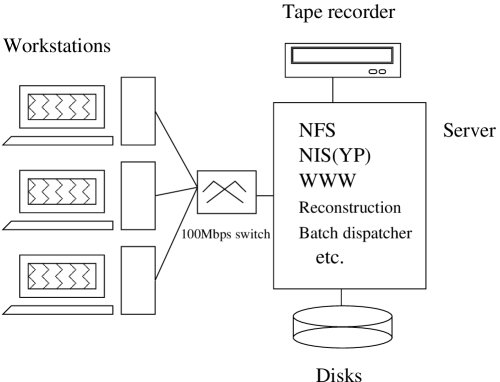
Figure 22: The computing system.

The computer system (Fig. 22) used for reconstruction and analysis of experimental data includes several desktop Pentium PCs running Linux 2.0 and a Sun Enterprise 450 server under Solaris 2.6 operating system. All computers are connected via 100 Mb Ethernet to a local network.

The server provides common software and user disk space for desktop PCs, along with batch system and network services. It also runs event reconstruction code at an average speed of about 150 events per second.

8 Monte Carlo simulation

The Monte Carlo simulation of the SND is based on UNIMOD [35] package. SND geometrical model comprises about 10000 distinct volumes. The primary generated particles are tracked through the detector media taking into account the following effects: ionization losses, multiple scattering, bremsstrahlung of electrons and positrons, Compton effect, $e^{+}e^{-}$ pair production by photons, photo-effect, unstable particles decays, interaction of stopped particles, nuclear interaction of hadrons. After that the signals produced in each detector element are simulated. To provide the adaptable account of experimental conditions: the electronics noise, signals pile up, the actual time and amplitude resolution of electronics channels. Broken channels are also taken into account during reconstruction of Monte Carlo events.

Comparison of experimental and simulated distributions are shown in Figs.24, 24.

9 Conclusions

The design and performance of the SND detector operating at VEPP-2M $e^{+}e^{-}$ collider since 1995 is described. During this time the total integrated luminosity of $\sim~{}25$ $pb^{-1}$ in the center-of-mass energy range $2E_{0}=0.4\div 1.4$ GeV was accumulated. New rare radiative decays $\phi\rightarrow\pi^{0}\pi^{0}\gamma$ [36], $\eta\pi^{0}\gamma$ [37] and OZI and G-parity suppressed decay $\phi\rightarrow\omega\pi^{0}$ [38] were observed. The $\phi\rightarrow\eta^{\prime}\gamma$ [39] decay existence was confirmed. Many other decays and hadronic production cross sections were measured with higher accuracy. More integrated luminosity is to be accumulated in the region of $\rho$ and $\omega$ mesons providing data for studies of their rare decays.

10 Acknowlegement

This work is supported in part by STP ‘Integration”, grant No.274 and Russian Fund for Basic Researches, grant No.96-15-96327.

Figure 5: Energy spectra for photons with energy $E_{0}=500$ MeV after cosmic calibration. $E$ is a measured energy.

Figure 6: Dependence of the most probable energy deposition on the photon energy.

Figure 7: Dependence of the calorimeter energy resolution on the photon energy, $\sigma_{E}/E(\%)=4.2\%/\sqrt[4]{E(\mbox{~{}GeV})}$. $E$ – photon energy, $\sigma_{E}/E$ – energy resolution obtained using $e^{+}e^{-}\rightarrow\gamma\gamma$ (dots) and $e^{+}e^{-}\rightarrow e^{+}e^{-}\gamma$ (circles) reactions.

Figure 8: Dependence of the angular resolution on the photon energy, $\sigma_{\phi}~{}=~{}0.82^{\circ}/\sqrt[]{E(\mbox{~{}GeV})}\oplus 0.63^{\circ}$. $E$ – photon energy

Figure 9: Two-photon invariant mass distribution in experimental $\phi\rightarrow\eta\gamma$ events.

Figure 10: Two-photon invariant mass distribution in experimental $\phi\rightarrow\pi^{+}\pi^{-}\pi^{0}$ events.

Figure 11: Spectra of the invariant masses of photon pairs in $e^{+}e^{-}\rightarrow\gamma\gamma\gamma$ events before (dots) and after (line) kinematic fit.

Figure 12: Energy deposition spectra for 385 MeV $e^{\pm}$ and $\pi^{\pm}$

.

Figure 13: Energy deposition in calorimeter first two layers vs total energy deposition for 385 MeV $e^{\pm}$ and $\pi^{\pm}$. $E$ – total energy deposition, $E_{1}+E_{2}$ – energy deposition in the first two layers

Figure 15: Electronics channel of Drift chambers (DC): (1) DC gas volume, (2) end cap, (3) pins for wire attachment, (4) field shaping wires, (5) sensitive wires, (6) field shaping strips, (7) sensitive strips, (HV) potential from high voltage divider, (CSA) charge sensitive amplifier, (PA) preamplifier, (A24) 24 channel amplitude to digital converter, (T2A) time and two amplitude to digital converters

Figure 16: The azimuthal acollinearity angle distribution for $e^{+}e^{-}~{}\rightarrow~{}e^{+}e^{-}$ events

Figure 17: $dE/dx$ distribution for events with charged particles in the center-of-mass energy range $2E_{0}\sim 1$ GeV

Figure 18: Muon system electronics: (AC) scintillation counters, (Tubes) streamer tube, (D) discriminator, (EXPAN) time expander, (Trigger) first-level trigger, ($\Sigma$) logical summator, (TDC) time to digital converter, (ADC) analog to digital converter

Figure 19: Time distribution of scintillation counters signals with respect to the beams collision time in $e^{+}e^{-}\rightarrow\mu^{+}\mu^{-}$ events at $2E_{0}\sim 1$ GeV. The cosmic muons background is also seen as a uniform contribution.

Figure 20: SND data acquisition system: KLUKVA crates, (FLT) first-level trigger, (IFLT) FLT interface modules, (Logic) modules of FLT logic and decision, (CAMAC) CAMAC crates

Figure 21: First-level trigger (FLT) structure scheme: (IFLT) FLT interface modules, (FADC) ADC “total energy deposition”, (A24) ADC, ($\Sigma$) – logical summator

Figure 23: Invariant mass distribution of $\pi^{0}$-mesons pairs from the $K_{S}\rightarrow\pi^{0}\pi^{0}$ decay.

Figure 24: Angle $\psi$ between pion pairs from the $K_{S}\rightarrow\pi^{+}\pi^{-}$ decay

References

- [1] A.N.Skrinsky, in Proc. of Workshop on physics and detectors for DANE, Frascati, Italy, April 4-7, 1995, p.3
- [2] Review of particle physics, Particle Data Group, Eur.Phys.J.C3,1-794(1998)
-
[3]
V.B.Golubev et al., Nucl. Instr. and Meth. 227 (1984) 467
M.D.Minakov et al., Instrum. Exp. Tech. 23 (1981) 868 - [4] V.B.Golubev et al., Instrum. Exp. Tech. 24 (1982) 1373
- [5] S.I.Dolinsky et al., Phys. Rep. 202 (1991) 99
- [6] V.M.Aulchenko et al., in Proc. of Workshop on physics and detectors for DANE, Frascati, Italy, April 9-12, 1991, p.605
-
[7]
V.M.Aulchenko et al., Preprint, Budker INP 95-56, Novosibirsk, 1995
V.M.Aulchenko et al., in Proc. of the 6th Int. Conf. on Hadron Spectroscopy, Manchester, UK, July 10-14, 1995, p.295 - [8] M.N.Achasov et al., Preprint, Budker INP 96-47, Novosibirsk, 1996
-
[9]
M.N.Achasov et al., Preprint, Budker INP 97-78, Novosibirsk, 1997.
M.N.Achasov et al., in Proc. of the 7th Int. Conf. on Hadron Spectroscopy, Brookhaven (BNL), USA, August 25-30, 1997, p.26 - [10] M.N.Achasov et al., Preprint, Budker INP 98-65, Novosibirsk, 1998
- [11] P.M.Beschastnov et al., Nucl. Instr. and Meth. A342 (1994) 477
- [12] M.N.Achasov et al., Nucl. Instr. and Meth. A401 (1997) 179
- [13] M.N.Achasov, et al. Nucl. Instr. and Meth. A411 (1998) 337
- [14] M.G.Bekishev, V.N.Ivanchenko, Nucl. Instr. and Meth. A361 (1995) 138
- [15] J.P.Berge et al., Rev. Scien. Instr. 32 (1961) 538
- [16] A.V.Bozhenok et al., in: Proc. of the 6th Int. Conf. on Instrumentation for Experiments at Colliders, Novosibirsk, Russia, 29 February - 6 March 1996; Nucl. Instr. and Meth. A379 (1996) 507
- [17] D.A.Bukin et al., Nucl. Instr. and Meth. A384 (1996) 360
- [18] B.O.Baibusinov et al., Preprint, Budker INP 91-96, Novosibirsk, 1991
- [19] A.D.Bukin et al., in Proc. of the Int. Conf. on Computing in High Energy Physics, Berlin, Germany, April 7 - 11, 1997.
- [20] V.M.Aulchenko et al., Nucl. Instr. and Meth. A409 (1998) 639
- [21] V.M.Aulchenko et al., Preprint, Budker INP 88-22, Novosibirsk, 1988
- [22] V.M.Aulchenko et al., Preprint, Budker INP 88-30, Novosibirsk, 1988
- [23] D.A.Bukin et al., in Proc. of the 6th Int. Conf on Instrumentation for Experiments at Colliders, Novosibirsk, Russia, 29 February -6 March 1996; Nucl. Instr. and Meth. A379 (1996) 545
- [24] D.A.Bukin et al., Preprint, Budker INP 98-15, Novosibirsk, 1998
- [25] D.A.Bukin et al., Preprint, Budker INP 98-29, Novosibirsk, 1998
- [26] V.N.Ivanchenko, Preprint, Budker INP 94-25, Novosibirsk, 1994
- [27] A.A.Korol, Preprint, Budker INP 94-62, Novosibirsk, 1994
- [28] I.A.Gaponenko, A.A.Salnikov, Preprint, Budker INP 98-39, Novosibirsk, 1998
- [29] A.D.Bukin, V.N.Ivanchenko, Preprint, Budker INP 93-81, Novosibirsk, 1993
- [30] R.Brun and D.Lienart, HBOOK User Guide – Version4, CERN program library Y250, 1988
- [31] R.Bock et al., HIGZ – High level interface to Graphics and ZEBRA, CERN program library Q120, 1988
- [32] R.Brun et al., PAW – physics analysis workstation, CERN program library Q121. CERN, Geneva, Switzerland, 1989
- [33] F.James, M.Roos, MINUIT – Function Minimization and Error Analysis, CERN program library D506, 1988.
- [34] E.A.Kuraev, V.S.Fadin, Sov. J. of Nucl. Phys., 41 (1985) 466.
- [35] A.D.Bukin et al., in Proc. of Workshop on Detector and Event Simulation in High Energy Physics, Amsterdam, April 8-12, 1991, p.79
- [36] M.N.Achasov et al., Phys. Lett. B440 (1998) 442
- [37] M.N.Achasov et al., Phys. Lett. B438 (1998) 441
- [38] M.N.Achasov et al., Phys. Lett. B449 (1999) 122
- [39] V.M.Aulchenko et al., JETP Letters 69 (1999) 87
.