A measurement of the $W$ boson mass using large rapidity electrons

Abstract

We present a measurement of the $W$ boson mass using data collected by the DØ experiment at the Fermilab Tevatron during 1994–1995. We identify $W$ bosons by their decays to $e\nu$ final states where the electron is detected in a forward calorimeter. We extract the $W$ boson mass, $M_{W}$, by fitting the transverse mass and transverse electron and neutrino momentum spectra from a sample of 11,089 $W\to e\nu$ decay candidates. We use a sample of 1,687 dielectron events, mostly due to $Z\to ee$ decays, to constrain our model of the detector response. Using the forward calorimeter data, we measure $M_{W}=80.691\pm 0.227$ GeV. Combining the forward calorimeter measurements with our previously published central calorimeter results, we obtain $M_{W}=80.482\pm 0.091$ GeV.

I Introduction

In this article we describe the first measurement [1] of the mass of the $W$ boson using electrons detected at large rapidities (i.e. between 1.5 and 2.5). We use data collected in 1994–1995 with the DØ detector [2] at the Fermilab Tevatron $p\overline{p}$ collider. This measurement performed with the DØ forward calorimeters [3] complements our previous measurements with central electrons [4, 5] and the more complete combined rapidity coverage gives useful constraints on model parameters that permit reduction of the systematic error, in addition to increasing the statistical precision.

The study of the properties of the $W$ boson began in 1983 with its discovery by the UA1 [6] and UA2 [7] collaborations at the CERN $p\overline{p}$ collider. Together with the discovery of the $Z$ boson in the same year [8, 9], it provided a direct confirmation of the unified description of the weak and electromagnetic interactions [10], which — together with the theory of the strong interaction, quantum chromodynamics (QCD) — now constitutes the standard model.

Since the $W$ and $Z$ bosons are carriers of the weak force, their properties are intimately coupled to the structure of the model. The properties of the $Z$ boson have been studied in great detail in $e^{+}e^{-}$ collisions [11]. The study of the $W$ boson has proven to be significantly more difficult, since it is charged and so cannot be resonantly produced in $e^{+}e^{-}$ collisions. Until recently its direct study has therefore been the realm of experiments at $p\overline{p}$ colliders [4, 5, 12, 13]. Direct measurements of the $W$ boson mass have also been carried out at LEP2 [14, 15, 16, 17] using nonresonant $W$ pair production. A summary of these measurements can be found in Table XI at the end of this article.

The standard model links the $W$ boson mass to other parameters,

$$M_{W}^{2}=\left({\pi\alpha(M_{Z}^{2})\over\sqrt{2}G_{F}}\right){M_{Z}^{2}\over(M_{Z}^{2}-M_{W}^{2})({1-\Delta r_{EW}})}\quad$$ (1)

in the “on shell” scheme [18]. Aside from the radiative corrections $\Delta r_{EW}$, the $W$ boson mass is thus determined by three precisely measured quantities, the mass of the $Z$ boson $M_{Z}$[11], the Fermi constant $G_{F}$ [19], and the electromagnetic coupling constant $\alpha$ evaluated at $Q^{2}=M_{Z}^{2}$ [19]:

$$M_{Z} = 91.1867\pm 0.0021\ \hbox{GeV},$$ (2)

$$G_{F} = (1.16639\pm 0.00001)\times 10^{-5}\ \hbox{GeV}^{-2}\quad,$$ (3)

$$\alpha = (128.88\pm 0.09)^{-1}\quad.$$ (4)

From the measured $W$ boson mass, we can derive the size of the radiative corrections $\Delta r_{EW}$. Within the framework of the standard model, these corrections are dominated by loops involving the top quark and the Higgs boson (see Fig. 1). The correction from the $t\overline{b}$ loop is substantial because of the large mass difference between the two quarks. It is proportional to $m_{t}^{2}$ for large values of the top quark mass $m_{t}$. Since $m_{t}$ has been measured [20, 21], this contribution can be calculated within the standard model. For a large Higgs boson mass, $m_{H}$, the correction from the Higgs loop is proportional to $\ln(m_{H})$. In extensions to the standard model, new particles may give rise to additional corrections to the value of $M_{W}$. In the minimal supersymmetric extension of the standard model (MSSM), for example, additional corrections can increase the predicted $W$ mass by up to 250 MeV [22].

FIG. 1.: Loop diagrams contributing to the $W$ boson mass.

A measurement of the $W$ boson mass therefore constitutes a test of the standard model. In conjunction with a measurement of the top quark mass, the standard model predicts $M_{W}$ up to a 200 MeV uncertainty due to the unknown Higgs boson mass. By comparing the standard model calculation to the measured value of the $W$ boson mass, we can constrain the mass of the Higgs boson, the agent of the electroweak symmetry breaking in the standard model that has up to now eluded experimental detection. A discrepancy with the range allowed by the standard model could indicate new physics. The experimental challenge is thus to measure the $W$ boson mass to sufficient precision, about 0.1%, to be sensitive to these corrections.

II Overview

A Conventions

We use a Cartesian coordinate system with the $z$-axis defined by the direction of the proton beam, the $x$-axis pointing radially out of the Tevatron ring, and the $y$-axis pointing up. A vector $\vec{p}$ is then defined in terms of its projections on these three axes, $p_{x}$, $p_{y}$, $p_{z}$. Since protons and antiprotons in the Tevatron are unpolarized, all physical processes are invariant with respect to rotations around the beam direction. It is therefore convenient to use a cylindrical coordinate system, in which the same vector is given by the magnitude of its component transverse to the beam direction, $p_{T}$, its azimuth $\phi$, and $p_{z}$. In $p\overline{p}$ collisions, the center-of-mass frame of the parton-parton collisions is approximately at rest in the plane transverse to the beam direction but has an undetermined motion along the beam direction. Therefore the plane transverse to the beam direction is of special importance, and sometimes we work with two-dimensional vectors defined in the $x$-$y$ plane. They are written with a subscript $T$, e.g. $\vec{p}_{T}$. We also use spherical coordinates by replacing $p_{z}$ with the polar angle $\theta$ (as measured between $p_{z}$ and the $z$-axis) or the pseudorapidity $\eta=-\ln\tan\left(\theta/2\right)$. The origin of the coordinate system is in general the reconstructed position of the $p\overline{p}$ interaction when describing the interaction, and the geometrical center of the detector when describing the detector. For convenience, we use units in which $c=\hbar=1$.

B $W$ and $Z$ Boson Production and Decay

In $p\overline{p}$ collisions at $\sqrt{s}=1.8$ TeV, $W$ and $Z$ bosons are produced predominantly through quark-antiquark annihilation. Figure 2 shows the lowest-order diagrams. The quarks in the initial state may radiate gluons which are usually very soft but may sometimes be energetic enough to give rise to hadron jets in the detector. In the reaction, the initial proton and antiproton break up and the fragments hadronize. We refer to everything except the vector boson and its decay products collectively as the underlying event. Since the initial proton and antiproton momentum vectors add to zero, the same must be true for the vector sum of all final state momenta and therefore the vector boson recoils against all particles in the underlying event. The sum of the transverse momenta of the recoiling particles must balance the transverse momentum of the boson, which is typically small compared to its mass but has a long tail to large values.

FIG. 2.: Lowest order diagrams for $W$ and $Z$ boson production.

We identify $W$ and $Z$ bosons by their leptonic decays. The DØ detector (Sec. III) is best suited for a precision measurement of electrons and positrons, and we therefore use the decay channel $W\to e\nu$ to measure the $W$ boson mass. $Z\to ee$ decays serve as an important calibration sample. About 11% of the $W$ bosons decay to $e\nu$ and about 3.3% of the $Z$ bosons decay to $ee$. The leptons typically have transverse momenta of about half the mass of the decaying boson and are well isolated from other large energy deposits in the calorimeter. Gauge vector boson decays are the dominant source of isolated high-$p_{T}$ leptons at the Tevatron, and therefore these decays allow us to select clean samples of $W$ and $Z$ boson decays.

C Event Characteristics

In events due to the process $p\overline{p}\to(W\to e\nu)+X$, where $X$ stands for the underlying event, we detect the electron and all particles recoiling against the $W$ boson with pseudorapidity $-4<\eta<4$. The neutrino escapes undetected. In the calorimeter we cannot resolve individual recoil particles, but we measure their energies summed over detector segments. Recoil particles with $|\eta|>4$ escape unmeasured through the beampipe, possibly carrying away substantial momentum along the beam direction. This means that we cannot measure the sum of the $z$-components of the recoil momenta, $u_{z}$, precisely. Since these particles escape at a very small angle with respect to the beam, their transverse momenta are typically small and neglecting them in the sum of the transverse recoil momenta, $\vec{u}_{T}$ causes a small amount of smearing of $\vec{u}_{T}$. We measure $\vec{u}_{T}$ by summing the observed energy flow vectorially over all detector segments. Thus, we reduce the reconstruction of every candidate event to a measurement of the electron momentum $\vec{p}(e)$ and $\vec{u}_{T}$.

Since the neutrino escapes undetected, the sum of all measured final state transverse momenta does not add to zero. The missing transverse momentum $\hbox to0.0pt{\kern 1.00006pt/\hss}\vec{p}_{T}$, required to balance the transverse momentum sum, is a measure of the transverse momentum of the neutrino. The neutrino momentum component along the beam direction cannot be determined, because $u_{z}$ is not measured well. The signature of a $W\to e\nu$ decay is therefore an isolated high-$p_{T}$ electron and large missing transverse momentum.

In the case of $Z\to ee$ decays, the signature consists of two isolated high-$p_{T}$ electrons and we measure the momenta of both leptons, $\vec{p}(e_{1})$ and $\vec{p}(e_{2})$, and $\vec{u}_{T}$ in the detector.

D Mass Measurement Strategy

Since $p_{z}(\nu)$ is unknown, we cannot reconstruct the $e\nu$ invariant mass for $W\to e\nu$ candidate events and therefore must resort to other kinematic variables for the mass measurement.

For recent measurements [12, 13, 5, 4] the transverse mass,

$$m_{T}=\sqrt{2p_{T}(e)p_{T}(\nu)\left(1-\cos\left(\phi(e)-\phi(\nu)\right)\right)}\quad,$$ (5)

was used. This variable has the advantage that its spectrum is relatively insensitive to the production dynamics of the $W$ boson. Corrections to $m_{T}$ due to the motion of the $W$ are of order $\left(q_{T}/M_{W}\right)^{2}$, where $q_{T}$ is the transverse momentum of the $W$ boson. It is also insensitive to selection biases that prefer certain event topologies (Sec. VI D). However, it makes use of the inferred neutrino $p_{T}$ and is therefore sensitive to the response of the detector to the recoil particles.

The electron $p_{T}$ spectrum provides an alternative measurement of the $W$ mass. It is measured with better resolution than the neutrino $p_{T}$ and is insensitive to the recoil momentum measurement. However, its shape is sensitive to the motion of the $W$ boson and receives corrections of order $q_{T}/M_{W}$. It thus requires a better understanding of the $W$ boson production dynamics than the $m_{T}$ spectrum does.

These effects are illustrated in Figs. 3 and 4, which show the effect of the motion of the $W$ bosons and the detector resolutions on the shapes of the $m_{T}$ and $p_{T}(e)$ spectra. The solid line shows the shape of the distribution before the detector simulation and with $q_{T}$=0. The points show the shape after $q_{T}$ is added to the system, and the shaded histogram also includes the detector simulation. We observe that the shape of the $m_{T}$ spectrum is dominated by detector resolutions and the shape of the $p_{T}(e)$ spectrum by the motion of the $W$ boson.

The shape of the neutrino $p_{T}$ spectrum is sensitive to both the $W$ boson production dynamics and the recoil momentum measurement. By performing the measurement using all three spectra, we provide a powerful cross check with complementary systematics.

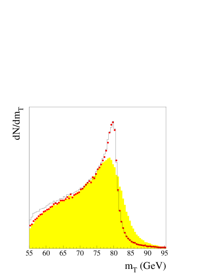
FIG. 3.: The $m_{T}$ spectrum for $W$ bosons with $q_{T}=0$ (——), with the correct $q_{T}$ distribution ($\bullet$), and with detector resolutions (shaded).

FIG. 4.: The $p_{T}(e)$ spectrum for $W$ bosons with $q_{T}=0$ (——), with the correct $q_{T}$ distribution ($\bullet$), and with detector resolutions (shaded).

All three spectra are equally sensitive to the electron energy response of the detector. We calibrate this response by forcing the observed dielectron mass peak in the $Z\to ee$ sample to agree with the known $Z$ mass[11] (Sec. VI). This means that we effectively measure the ratio of $W$ and $Z$ masses, which is equivalent to a measurement of the $W$ mass because the $Z$ mass is known precisely.

To carry out these measurements, we perform a maximum likelihood fit to the spectra. Since the shape of the spectra, including all the experimental effects, cannot be computed analytically, we need a Monte Carlo simulation program that can predict the shape of the spectra as a function of the $W$ mass. To measure the $W$ mass to a precision of order 100 MeV, we wish to estimate individual systematic effects with a statistical error of 5 MeV. Our technique requires a Monte Carlo sample of 10 million accepted $W$ bosons for each such effect. The program therefore must be capable of generating large event samples in a reasonable time. We obtain the required Monte Carlo statistics by employing a parameterized model of the detector response.

We next summarize the aspects of the accelerator and detector that are important for our measurement (Sec. III). Then we describe the data selection (Sec. IV) and the fast Monte Carlo model (Sec. V). Most parameters in the model are determined from our data. We describe the determination of the various components of the Monte Carlo model in Secs. VI-IX. After tuning the model, we fit the kinematic spectra (Sec. X), perform some consistency checks (Sec. XI), and discuss the systematic uncertainties (Sec. XII). We present the error analysis in Sec. XIII, and summarize the results and present the conclusions in Sec. XIV.

III Experimental Method

A Accelerator

During the data run, the Fermilab Tevatron[23] collided proton and antiproton beams at a center-of-mass energy of $\sqrt{s}=1.8$ TeV. Six bunches each of protons and antiprotons circulated around the ring in opposite directions. Bunches crossed at the intersection regions every 3.5 $\mu$s. During the 1994–1995 running period, the accelerator reached a peak luminosity of $2.5\times 10^{31}\hbox{cm}^{-2}\hbox{s}^{-1}$ and delivered an integrated luminosity of about 100 pb^-1. The beam interaction region at DØ was at the center of the detector with an r.m.s. length of 27 cm.

The Tevatron tunnel also housed a 150 GeV proton synchrotron, called the Main Ring, used as an injector for the Tevatron and accelerated protons for antiproton production during collider operation. Since the Main Ring beampipe passed through the outer section of the DØ calorimeter, passing proton bunches gave rise to backgrounds in the detector. We eliminated this background using timing cuts based on the accelerator clock signal.

B Detector

1 Overview

The DØ detector consists of three major subsystems: an inner tracking detector, a calorimeter, and a muon spectrometer. It is described in detail in Ref. [2]. We describe only the features that are most important for this measurement.

2 Inner Tracking Detector

The inner tracking detector is designed to measure the trajectories of charged particles. It consists of a vertex drift chamber, a transition radiation detector, a central drift chamber (CDC), and two forward drift chambers (FDC). There is no central magnetic field. The CDC covers the region $|\eta|<1.0$. The FDC covers the region $1.4<|\eta|<3.0$. Each FDC consists of three separate chambers: a $\Phi$ module, with radial wires which measures the $\phi$ coordinate, sandwiched between a pair of $\Theta$ modules which measure (approximately) the radial coordinate. Figure 5 shows one of the two FDC detectors.

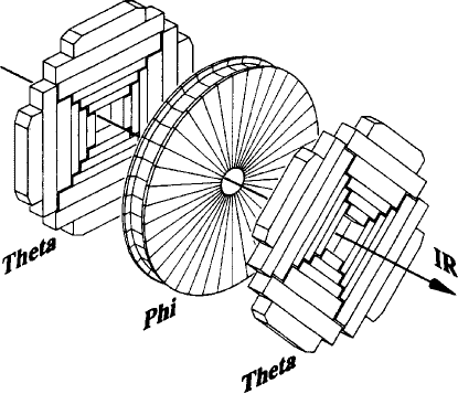
FIG. 5.: An exploded view of a DØ forward drift chamber (FDC).

3 Calorimeter

The uranium/liquid-argon sampling calorimeter (Fig. 6) is the most important part of the detector for this measurement. There are three calorimeters: a central calorimeter (CC) and two end calorimeters (EC), each housed in its own cryostat. Each is segmented into an electromagnetic (EM) section, a fine hadronic (FH) section, and a coarse hadronic (CH) section, with increasingly coarser sampling.

FIG. 6.: A cutaway view of the DØ calorimeter and tracking system.

The ECEM section (Fig. 7) has a monolithic construction of alternating uranium plates, liquid-argon gaps, and multilayer printed-circuit readout boards. Each end calorimeter is divided into about 1000 pseudo-projective towers, each covering 0.1$\times$0.1 in $\eta\times\phi$. The EM section is segmented into four layers, 0.3, 2.6, 7.9, and 9.3 radiation lengths thick. The third layer, in which electromagnetic showers typically reach their maximum, is transversely segmented into cells covering 0.05$\times$0.05 in $\eta\times\phi$. The EC hadronic section is segmented into five layers. The entire calorimeter is 7–9 nuclear interaction lengths thick. There are no projective cracks in the calorimeter and it provides hermetic and almost uniform coverage for particles with $|\eta|<4$.

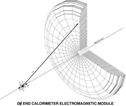
FIG. 7.: The ECEM section of an end calorimeter.

The signals from arrays of 2$\times$2 calorimeter towers covering 0.2$\times$0.2 in $\eta\times\phi$ are added together electronically for the EM section alone and for the EM and hadronic sections together, and shaped with a fast rise time for use in the Level 1 trigger. We refer to these arrays of 2$\times$2 calorimeter towers as “trigger towers.”

The liquid argon has unit gain and the end calorimeter response was extremely stable during the entire run. The liquid-argon response was monitored with radioactive sources of $\alpha$ and $\beta$ particles throughout the run, as were the gains and pedestals of all readout channels. Details can be found in Ref. [24].

The ECEM calorimeter provides a measurement of energy and position of the electrons from the $W$ and $Z$ boson decays. Due to the fine segmentation of the third layer, we can measure the position of the shower centroid with a precision of about 1 mm in the azimuthal and radial directions.

We have studied the response of the ECEM calorimeter to electrons in beam tests [3, 25]. To reconstruct the electron energy we add the signals $a_{i}$ observed in each EM layer ($i=1,\ldots,4$) and the first FH layer ($i=5$) of an array of 5$\times$5 calorimeter towers, centered on the most energetic tower, weighted by a layer-dependent sampling weight $s_{i}$,

$$E=A\sum_{i=1}^{5}s_{i}a_{i}-\delta_{\rm EC}\quad.$$ (6)

To determine the sampling weights we minimize

$$\chi^{2}=\sum{(p-E)^{2}\over\sigma_{\rm EM}^{2}}\quad,$$ (7)

where the sum runs over all events, $\sigma_{\rm EM}$ is the resolution given in Eq. 8 and $p$ is the beam momentum. We obtain $A=3.74$ MeV/ADC count, $\delta_{\rm EC}=-300$ MeV, $s_{1}=1.47$, $s_{2}=1.00$, $s_{4}=1.10$, and $s_{5}=1.67$. We arbitrarily fix $s_{3}=1$. The value of $\delta_{\rm EC}$ depends on the amount of uninstrumented material in front of the calorimeter. The parameters $s_{1}$ to $s_{4}$ weight the four EM layers and $s_{5}$ the first FH layer. Figure 8 shows the fractional deviation of $E$ as a function of the beam momentum $p$. Above 20 GeV the non-linearity is less than 0.1%.

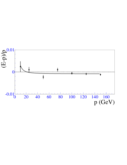
FIG. 8.: The fractional deviation of the reconstructed electron energy from the beam momentum from beam tests of an ECEM module.

The fractional energy resolution can be parameterized as a function of electron energy using constant, sampling, and noise terms as

$$\left({\sigma_{\rm EM}\over E}\right)^{2}=c_{\rm EM}^{2}+\left({s_{\rm EM}\over\sqrt{E}}\right)^{2}+\left({n_{\rm EM}\over E}\right)^{2},$$ (8)

with $c_{\rm EM}=0.003$, $s_{\rm EM}=0.157$ GeV^1/2 and $n_{\rm EM}=0.29$ GeV in the end calorimeters, as measured in beam tests [3, 25].

4 Muon Spectrometer

The DØ muon spectrometer consists of five separate solid-iron toroidal magnets, together with sets of proportional drift tube chambers to measure the track coordinates. The central toroid covers the region $\mid\!\eta\!\mid\leq 1$, two end toroids cover $1<\mid\!\eta\!\mid\leq 2.5$, and the small-angle muon system covers $2.5<\mid\!\eta\!\mid\leq 3.6$. There is one layer of chambers inside the toroids and two layers outside for detecting and reconstructing the trajectory and the momentum of muons.

5 Luminosity Monitor

Two arrays of scintillator hodoscopes, mounted in front of the EC cryostats, register hits with a 220 ps time resolution. They serve to detect the occurance of an inelastic $p\overline{p}$ interaction. The particles from the breakup of the proton give rise to hits in the hodoscopes on one side of the detector that are tightly clustered in time. For events with a single interaction, the location of the interaction vertex can be determined with a resolution of 3 cm from the time difference between the hits on the two sides of the detector for use in the Level 2 trigger. This array is also called the Level 0 trigger because the detection of an inelastic $p\overline{p}$ interaction is required for most triggers.

6 Trigger

Readout of the detector is controlled by a two-level trigger system. Level 1 consists of an and-or network that can be programmed to trigger on a $p\overline{p}$ crossing if a number of preselected conditions are satisfied. The Level 1 trigger decision is taken within the 3.5 $\mu$s time interval between crossings. As an extension to Level 1, a trigger processor (Level 1.5) may be invoked to execute simple algorithms on the limited information available at the time of a Level 1 accept. For electrons, the processor uses the energy deposits in each trigger tower as inputs. The detector cannot accept any triggers until the Level 1.5 processor completes execution and accepts or rejects the event.

Level 2 of the trigger consists of a farm of 48 VAXstation 4000’s. At this level, the complete event is available. More sophisticated algorithms refine the trigger decisions and events are accepted based on preprogrammed conditions. Events accepted by Level 2 are written to magnetic tape for offline reconstruction.

IV Data Selection

A Trigger

The conditions required at trigger Level 1 for $W$ and $Z$ boson candidates are:

• $\underline{\hbox{$p\overline{p}$\ interaction:}}$ Level 0 hodoscopes register hits consistent with a $p\overline{p}$ interaction. Using monitor trigger data, the efficiency of this condition has been measured to be 98.6%.

• $\underline{\hbox{Main Ring Veto:}}$ No Main Ring proton bunch passes through the detector within 800 ns of the $p\overline{p}$ crossing and no protons were injected into the Main Ring less than 400 ms before the $p\overline{p}$ crossing.

• $\underline{\hbox{EM trigger towers:}}$ There are one or more EM trigger towers with $E\sin\theta>T$, where $E$ is the energy measured in the tower, $\theta$ is the polar angle of the tower with the beam measured from the center of the detector, and $T$ is a programmable threshold. This requirement is fully efficient for electrons with $p_{T}>2T$.

The Level 1.5 processor recomputes the transverse electron energy by adding the adjacent EM trigger tower with the largest signal to the EM trigger tower that exceeded the Level 1 threshold. In addition, the signal in the EM trigger tower that exceeded the Level 1 threshold must constitute at least 85% of the signal registered in this tower if the hadronic layers are also included. This EM fraction requirement is fully efficient for electron candidates that pass our offline selection (Sec. IV D).

Level 2 uses the EM trigger tower that exceeded the Level 1 threshold as a starting point. The Level 2 algorithm finds the most energetic of the four calorimeter towers that make up the trigger tower, and sums the energy in the EM sections of a 3$\times$3 array of calorimeter towers around it. It checks the longitudinal shower shape by applying cuts on the fraction of the energy in the different EM layers. The transverse shower shape is characterized by the energy deposition pattern in the third EM layer. The difference between the energies in concentric regions covering 0.25$\times$0.25 and 0.15$\times$0.15 in $\eta\times\phi$ must be consistent with an electron. Level 2 also imposes an isolation condition requiring

$$\frac{\sum_{i}E_{i}\sin\theta_{i}-p_{T}}{p_{T}}<0.15\quad,$$ (9)

where $E_{i}$ and $\theta_{i}$ are the energy and polar angle of cell $i$, the sum runs over all cells within a cone of radius $R=\sqrt{\Delta\phi^{2}+\Delta\eta^{2}}=0.4$ around the electron direction and $p_{T}$ is the transverse momentum of the electron [26].

The $p_{T}$ of the electron computed at Level 2 is based on its energy and the $z$-position of the interaction vertex measured by the Level 0 hodoscopes. Level 2 accepts events that have a minimum number of EM clusters that satisfy the shape cuts and have $p_{T}$ above a preprogrammed threshold. Figure 9 shows the measured relative efficiency of the Level 2 electron filter for forward electrons versus electron $p_{T}$ for a Level 2 $p_{T}$ threshold of 20 GeV. We determine this efficiency using $Z$ boson data taken with a lower threshold value (16 GeV) for one electron. The efficiency is the fraction of electrons above a Level 2 $p_{T}$ threshold of 20 GeV. The curve is the parameterization used in the fast Monte Carlo (see Sec. V).

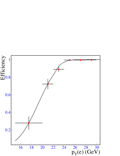
FIG. 9.: The relative efficiency of the Level 2 electron filter for a threshold of 20 GeV for EC electrons, as a function of the $p_{T}(e)$ computed offline for the $W$ boson mass analysis.

Level 2 also computes the missing transverse momentum based on the energy registered in each calorimeter cell and the vertex $z$-position as measured by the Level 0 hodoscopes. The level 2 $W$ boson trigger requires minimum $\hbox to0.0pt{\kern 1.00006pt/\hss}p_{T}$ of 15 GeV. We determine the efficiency curve for a 15 GeV Level 2 $\hbox to0.0pt{\kern 1.00006pt/\hss}p_{T}$ requirement from data taken without the Level 2 $\hbox to0.0pt{\kern 1.00006pt/\hss}p_{T}$ condition. Figure 10 shows the measured efficiency versus $p_{T}(\nu)$ as computed for the $W$ mass analysis, when the electron is detected in the end calorimeters. The curve is the parameterization used in the fast Monte Carlo.

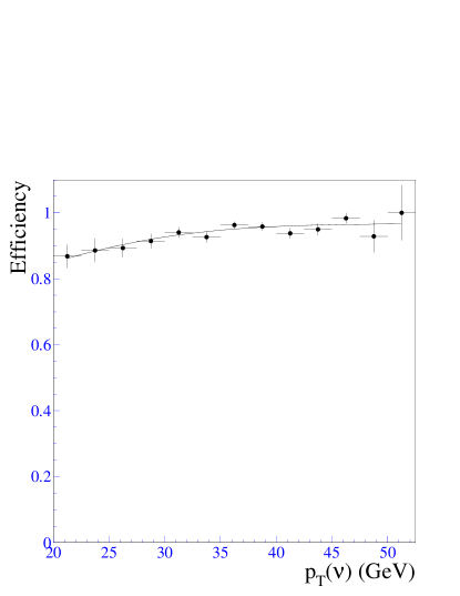
FIG. 10.: The efficiency of a 15 GeV Level 2 $\hbox to0.0pt{\kern 1.00006pt/\hss}p_{T}$ requirement for EC electrons, as a function of the $p_{T}(\nu)$ computed for the $W$ boson mass analysis.

B Reconstruction

1 Electron

We identify electrons as clusters of adjacent calorimeter cells with significant energy deposits. Only clusters with at least 90% of their energy in the EM section and at least 60% of their energy in the most energetic calorimeter tower are considered as electron candidates. For most electrons we also reconstruct a track in the CDC or FDC that points towards the centroid of the cluster.

We compute the forward electron energy $E(e)$ from the signals in all cells of the EM layers and the first FH layer whose centers lie within a projective cone of radius 20 cm and centered at the cluster centroid. In the computation we use the sampling weights and calibration constants determined using the test-beam data (Sec. III B 3), except for the overall energy scale $A$ and the offset $\delta_{\rm EC}$, which we take from an in situ calibration (Sec. VI E).

The calorimeter shower centroid position ($x_{\rm cal}$, $y_{\rm cal}$, $z_{\rm cal}$), the track coordinates ($x_{\rm trk}$, $y_{\rm trk}$, $z_{\rm trk}$), and the proton beam trajectory define the electron angle. We determine the position of the electron shower centroid $\vec{x}_{\rm cal}=(x_{\rm cal},y_{\rm cal},z_{\rm cal})$ in the calorimeter from the energy depositions in the third EM layer by computing the weighted mean of the positions $\vec{x}_{i}$ of the cell centers,

$$\vec{x}_{\rm cal}={\sum_{i}w_{i}\vec{x}_{i}\over\sum_{i}w_{i}}\quad.$$ (10)

The weights are given by

$$w_{i}=\max\left(0,w_{0}+\log\left({E_{i}\over E(e)}\right)\right)\quad,$$ (11)

where $E_{i}$ is the energy in cell $i$, $w_{0}$ is a parameter which depends upon $\eta(e)$, and $E(e)$ is the energy of the electron. The FDC track coordinates are reported at a fixed $z$ position using a straight line fit to all the drift chamber hits on the track. The calibration of the radial coordinates measured in the cylindrical coordinate system contributes a systematic uncertainty to the $W$ boson mass measurement. Using tracks from many events reconstructed in the vertex drift chamber, we measure the beam trajectory for every run. The closest approach to the beam trajectory of the line through the shower centroid and the track coordinates defines the $z$-position of the interaction vertex ($z_{\rm vtx}$). The beam trajectory provides ($x_{\rm vtx}$,$y_{\rm vtx}$). In $Z\to ee$ events, we may have two electron candidates with tracks. In this case we take the point determined from the more central electron as the interaction vertex, because this gives better resolution. Using only the electron track to determine the position of the interaction vertex, rather than all tracks in the event, makes the resolution of this measurement less sensitive to the luminosity and avoids confusion between vertices in events with more than one $p\overline{p}$ interaction.

We then define the azimuth $\phi(e)$ and the polar angle $\theta(e)$ of the electron using the vertex and the shower centroid positions

$$\tan\phi(e) = {y_{\rm cal}-y_{\rm vtx}\over x_{\rm cal}-x_{\rm vtx}}\quad,$$ (12)

$$\tan\theta(e) = {\sqrt{x_{\rm cal}^{2}+y_{\rm cal}^{2}}-\sqrt{x_{\rm vtx}^{2}+y_{\rm vtx}^{2}}\over z_{\rm cal}-z_{\rm vtx}}\quad.$$ (13)

Neglecting the electron mass, the momentum of the electron is given by

$$\vec{p}(e)=E(e)\left(\begin{array}[]{l}\sin\theta(e)\cos\phi(e)\\ \sin\theta(e)\sin\phi(e)\\ \cos\theta(e)\end{array}\right).$$ (14)

2 Recoil

We reconstruct the transverse momentum of all particles recoiling against the $W$ or $Z$ boson by taking the vector sum

$$\vec{u}_{T}=\sum_{i}E_{i}\sin\theta_{i}\left(\begin{array}[]{c}\cos\phi_{i}\\ \sin\phi_{i}\end{array}\right),$$ (15)

where the sum runs over all calorimeter cells that were read out, except those that belong to electron cones. $E_{i}$ are the cell energies, and $\phi_{i}$ and $\theta_{i}$ are the azimuth and polar angle of the center of cell $i$ with respect to the interaction vertex.

3 Derived Quantities

In the case of $Z\to ee$ decays, we define the dielectron momentum

$$\vec{p}(ee)=\vec{p}(e_{1})+\vec{p}(e_{2})$$ (16)

and the dielectron invariant mass

$$m(ee)=\sqrt{2E(e_{1})E(e_{2})(1-\cos\omega)}\quad,$$ (17)

where $\omega$ is the opening angle between the two electrons. It is useful to define a coordinate system in the plane transverse to the beam that depends only on the electron directions. We follow the conventions first introduced by UA2[12] and call the axis along the inner bisector of the transverse directions of the two electrons the $\eta$-axis and the axis perpendicular to that the $\xi$-axis. Projections on these axes are denoted with subscripts $\eta$ or $\xi$. Figure 11 illustrates these definitions.

FIG. 11.: Illustration of momentum vectors in the transverse plane for $Z\to ee$ candidates. The vectors drawn as thick lines are directly measured.

In the case of $W\to e\nu$ decays, we define the transverse neutrino momentum

$$\vec{p}_{T}(\nu)=-\vec{p}_{T}(e)-\vec{u}_{T}$$ (18)

and the transverse mass (Eq. 5). Useful quantities are the projection of the transverse recoil momentum on the transverse component of the electron direction,

$$u_{\parallel}=\vec{u}_{T}\cdot\hat{p}_{T}(e)\quad,$$ (19)

and the projection perpendicular to the transverse component of the electron direction,

$$u_{\perp}=\vec{u}_{T}\cdot(\hat{p}_{T}(e)\times\hat{z})\quad.$$ (20)

Figure 12 illustrates these definitions.

FIG. 12.: Illustration of momentum vectors in the transverse plane for $W\to e\nu$  candidates. The vectors drawn as thick lines are directly measured.

C Electron Identification

1 Fiducial Cuts

Electrons in the ECEM are defined by the pseudorapidity $\eta$ of the cluster centroid position with respect to the center of the detector. We define forward electrons by $1.5\leq\mid\eta_{\rm det}(e)\mid\leq 2.5$.

2 Quality Variables

We test how well the shape of a cluster agrees with that expected for an electromagnetic shower by computing a quality variable ($\chi^{2}$) for all cell energies using a 41-dimensional covariance matrix. The covariance matrix was determined from geant-based [27] simulations [28] that were tuned to agree with extensive test beam measurements.

To determine how well a track matches a cluster, we extrapolate the track to the third EM layer in the end calorimeter and compute the distance between the extrapolated track and the cluster centroid in the azimuthal direction, $\Delta s$, and in the radial direction, $\Delta\rho$. The variable

$$\sigma_{\rm trk}^{2}=\left({\Delta s\over\delta s}\right)^{2}+\left({\Delta\rho\over\delta\rho}\right)^{2},$$ (21)

quantifies the quality of the match. The parameters $\delta s=0.25$ cm and $\delta\rho=1.0$ cm are the resolutions with which $\Delta s$ and $\Delta\rho$ are measured, as determined using the end calorimeter electrons from $W\to e\nu$ decays.

In the EC, electrons must have a matched track in the forward drift chamber to suppress background due to misidentification. In the CC, we define “tight” and “loose” criteria. The tight criteria require a matched track in the CDC, defined as the track with the smallest $\sigma_{\rm trk}$. The loose criteria do not require a matched track and help increase the electron finding efficiency for $Z\to ee$ decays with at least one central electron.

The isolation fraction is defined as

$$f_{\rm iso}={E_{\rm cone}-E_{\rm core}\over E_{\rm core}},$$ (22)

where $E_{\rm cone}$ is the energy in a cone of radius $R=0.4$ around the direction of the electron, summed over the entire depth of the calorimeter, and $E_{\rm core}$ is the energy in a cone of $R=0.2$, summed over the EM calorimeter only.

We use the $dE/dx$ information provided by the FDC on the tracks associated with the EM calorimeter cluster. The $dE/dx$ information helps to distinguish between singly-ionizing electron tracks and doubly-ionizing tracks from photon conversions.

We identify electron candidates in the forward detectors by making loose cuts on the shower shape $\chi^{2}$, the track-cluster match quality, and the shower electromagnetic energy fraction. The electromagnetic energy fraction is the ratio of the cluster energy measured in the electromagnetic calorimeter to the total cluster energy (including the hadronic calorimeter), and is a measure of the longitudinal shower profile. We then use a cut on a 4-variable likelihood ratio $\lambda_{4}$ which combines the information in these variables and the track $dE/dx$ into a single variable. The final cut on the likelihood ratio $\lambda_{4}$ gives the maximum discrimination between electrons and jet background, i.e. gives the maximum background rejection for any given electron selection efficiency.

Figure 13 shows the distributions of the quality variables for electrons in the EC data; the arrows indicate the cut values. Table I summarizes the electron selection criteria.

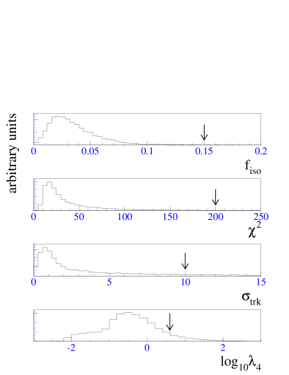
FIG. 13.: Distributions of the EC electron identification variables for $W\to e\nu$ candidates in the data. The arrows indicate the cut values.

TABLE I.: Electron selection criteria. $\Delta\phi_{\rm cal}$ is the difference in azimuthal angle between the cluster centroid and the CC module edge.

variable	CC (loose)	CC (tight)	EC (tight)
fiducial cuts	$|\Delta\phi_{\rm cal}|>0.02$	$|\Delta\phi_{\rm cal}|>0.02$	—
	$|z_{\rm cal}|<108$ cm	$|z_{\rm cal}|<108$ cm	$1.5\leq|\eta|\leq 2.5$
	—	$|z_{\rm trk}|<80$ cm	—
shower shape	$\chi^{2}<100$	$\chi^{2}<100$	$\chi^{2}<200$
isolation	$f_{\rm iso}<0.15$	$f_{\rm iso}<0.15$	$f_{\rm iso}<0.15$
track match	—	$\sigma_{\rm trk}<5$	$\sigma_{\rm trk}<10$
4-variable
likelihood ratio	—	—	$\lambda_{4}<$4

D Data Samples

The data were collected during the 1994–1995 Tevatron run. After the removal of runs in which parts of the detector were not operating adequately, the data correspond to an integrated luminosity of 82 pb^-1. We select $W$ boson decay candidates by requiring:

Level 1:	$p\overline{p}$ interaction
	Main Ring Veto
	EM trigger tower above 10 GeV
Level 1.5:	$\geq 1$ EM cluster above 15 GeV
Level 2:	electron candidate with $p_{T}>20$ GeV
	momentum imbalance $\mbox{$\hbox to0.0pt{\kern 1.00006pt/\hss}p_{T}$}>15$ GeV
offline:	$\geq 1$ tight electron candidate in EC
	$p_{T}(e)>30$ GeV
	$p_{T}(\nu)>30$ GeV
	$u_{T}<15$ GeV

This selection gives us 11,089 $W$ boson candidates. We select $Z$ boson decay candidates by requiring:

Level 1:	$p\overline{p}$ interaction
	$\geq 2$ EM trigger towers above 7 GeV
Level 1.5:	$\geq 1$ EM cluster above 10 GeV
Level 2:	$\geq 2$ electron candidates with $p_{T}>20$ GeV
offline:	$\geq 2$ electron candidates
	$p_{T}(e)>30$ GeV (EC)
	or $p_{T}(e)>25$ GeV (CC)

We accept $Z\to ee$ decays with at least one electron candidate in the EC and the other in the CC or the EC. EC candidates must pass the tight electron selection criteria. A CC candidate may pass only the loose criteria. We use the 1,687 events with at least one electron in the EC (CC/EC + EC/EC $Z$ samples) to calibrate the calorimeter response to electrons (Sec. VI). These events need not pass the Main Ring Veto cut because Main Ring background does not affect the EM calorimeter. Of these events, those that do pass the Main Ring Veto have been used to calibrate the recoil momentum response. The events for which both electrons are in the EC (EC/EC $Z$ sample) and which pass the Main Ring Veto serve to check the calibration of the recoil response (Sec. VII). Table II summarizes the data samples.

TABLE II.: Number of $W$ and $Z$ boson candidate events.

channel	$Z\to ee$		$W\to e\nu$
fiducial region of electrons	CC/EC	EC/EC	EC
	1265	422	11089

Figure 14 shows the luminosity of the colliding beams during the $W$ and $Z$ boson data collection.

FIG. 14.: The instantaneous luminosity distribution of the $W$ (top) and the $Z$ (bottom) boson samples.

On several occasions we use a sample of 295,000 random $p\overline{p}$ interaction events for calibration purposes. We collected these data concurrently with the $W$ and $Z$ signal data, requiring only a $p\overline{p}$ interaction at Level 1. We refer to these data as “minimum bias events.”

V Fast Monte Carlo Model

A Overview

The fast Monte Carlo model consists of three parts. First we simulate the production of the $W$ or $Z$ boson by generating the boson four-momentum and other characteristics of the event such as the $z$-position of the interaction vertex and the luminosity. The event luminosity is required for luminosity-dependent parametrizations in the detector simulation. Then we simulate the decay of the boson. At this point we know the true $p_{T}$ of the boson and the momenta of its decay products. We next apply a parameterized detector model to these momenta to simulate the observed transverse recoil momentum and the observed electron momenta.

Our fast Monte Carlo program is very similar to the one used in our published CC analysis [4], with some modifications in the simulation of forward electron events.

B Vector Boson Production

To specify the production dynamics of vector bosons in $p\overline{p}$ collisions completely, we need to know the differential production cross section in mass $Q$, rapidity $y$, and transverse momentum $q_{T}$ of the produced $W$ bosons. To speed up the event generation, we factorize this into

$${d^{3}\sigma\over dq_{T}^{2}dydQ}\approx\left.{d^{2}\sigma\over dq_{T}^{2}dy}\right|_{Q^{2}=M_{W}^{2}}\times{d\sigma\over dQ}$$ (23)

to generate $q_{T}$, $y$, and $Q$ of the bosons.

For $p\overline{p}$ collisions, the vector boson production cross section is given by the parton cross section $\widetilde{\sigma}_{i,j}$ convoluted with the parton distribution functions (pdf) $f(x,Q^{2})$ and summed over parton flavors $i,j$:

$${d^{2}\sigma\over dq_{T}^{2}dy} = \sum_{i,j}\int dx_{1}\int dx_{2}f_{i}(x_{1},Q^{2})f_{j}(x_{2},Q^{2})$$ (25)

$$\ \ \delta(sx_{1}x_{2}-Q^{2}){d^{2}\widetilde{\sigma}_{i,j}\over dq_{T}^{2}dy}\quad.$$

The cross section $d^{2}\sigma/dq_{T}^{2}dy|_{Q^{2}=M_{W}^{2}}$ has been computed by several authors [29, 30] using a perturbative calculation [31] for the high-$q_{T}$ regime and the Collins-Soper resummation formalism [32, 33] for the low-$q_{T}$ regime. We use the code provided by the authors of Ref. [29] and the MRST parton distribution functions [34] to compute the cross section. The production of $WW$, $WZ$ and $W\gamma$ is suppressed by three orders of magnitude compared to inclusive W production.

We use a Breit-Wigner curve with a mass-dependent width for the line shape of the $W$ boson. The intrinsic width of the $W$ is $\Gamma_{W}=2.062\pm 0.059$ GeV [35]. The line shape is skewed due to the momentum distribution of the quarks inside the proton and antiproton. The mass spectrum is given by

$${d\sigma\over dQ}={\cal L}_{q\overline{q}}(Q){Q^{2}\over(Q^{2}-M_{W}^{2})^{2}+{Q^{4}\Gamma_{W}^{2}\over M_{W}^{2}}}\quad.$$ (26)

We call

$${\cal L}_{q\overline{q}}(Q)={2Q\over s}\sum_{i,j}\int_{Q^{2}/s}^{1}{dx\over x}f_{i}(x,Q^{2})f_{j}(Q^{2}/sx,Q^{2})$$ (27)

the parton luminosity. To evaluate it, we generate $W\to e\nu$ events using the herwig Monte Carlo event generator [36], interfaced with pdflib [37], and select the events subject to the same fiducial cuts as for the $W$ and $Z$ boson samples with at least one electron in EC. We plot the mass spectrum divided by the intrinsic line shape of the $W$ boson. The result is proportional to the parton luminosity, and we parameterize the shape of the spectrum with the function [5]

$${\cal L}_{q\overline{q}}(Q)={e^{-\beta Q}\over Q}\quad.$$ (28)

Table III shows the parton luminosity slope $\beta$ for $W$ and $Z$ events for the different topologies. The value of $\beta$ depends on the rapidity distribution of the $W$ and $Z$ bosons, which is restricted by the fiducial cuts that we impose on the decay leptons. The values of $\beta$ given in Table III are for the rapidity distributions of $W$ and $Z$ bosons that satisfy the fiducial cuts given in Sec. IV. The uncertainty in $\beta$ is about 0.001 GeV^-1, due to Monte Carlo statistics and uncertainties in the acceptance.

TABLE III.: Parton luminosity slope $\beta$ in the $W$ and $Z$ boson production model. The $\beta$ value is given for $W\to e\nu$ decays with the electron in the EC and for $Z\to ee$ decays with at least one electron in the EC.

	$Z$ production	$W$ production
	$\beta$ (GeV-1)	$\beta$ (GeV-1)
CC/EC	$9.9\times 10^{-3}$	—
EC/EC	$19.9\times 10^{-3}$	—
EC	—	$16.9\times 10^{-3}$

Bosons can be produced by the annihilation of two valence quarks, two sea quarks, or one valence quark and one sea quark. Using the herwig events, we evaluate the fraction $f_{\rm ss}$ of bosons produced by the annihilation of two sea quarks. We find $f_{\rm ss}=0.207$, independent of the boson topology.

To generate the boson four-momenta, we treat $d\sigma/dQ$ and $d^{2}\sigma/dq_{T}^{2}dy$ as probability density functions and pick $Q$ from the former and a pair of $y$ and $q_{T}$ values from the latter. For a fraction $f_{\rm ss}$ the boson helicity is $+1$ or $-1$ with equal probability. The remaining $W$ bosons always have helicity $-1$. Finally, we pick the $z$-position of the interaction vertex from a Gaussian distribution centered at $z=0$ with a standard deviation of 27 cm and a luminosity for each event from the histogram in Fig. 14.

C Vector Boson Decay

At lowest order, the $W^{\pm}$ boson is fully polarized along the beam direction due to the $V\mp A$ coupling of the charged current. The resulting angular distribution of the charged lepton in the $W$ boson rest frame is given by

$${d\sigma\over d\cos\theta^{*}}\propto(1-\lambda q\cos\theta^{*})^{2}\quad,$$ (29)

where $\lambda$ is the helicity of the $W$ boson with respect to the proton direction, $q$ is the charge of the lepton, and $\theta^{*}$ is the angle between the charged lepton and proton beam directions in the $W$ rest frame. The spin of the $W$ boson points along the direction of the incoming antiquark. Most of the time, the quark comes from the proton and the antiquark from the antiproton, so that $\lambda=-1$. Only if both quark and antiquark come from the sea of the proton and antiproton, is there a 50% chance that the quark comes from the antiproton and the antiquark from the proton and in that case $\lambda=1$ (see Fig. 15).

FIG. 15.: Polarization of the $W$ boson produced in $p\overline{p}$ collisions if the quark comes from the proton (left) and if the antiquark comes from the proton (right). The short thick arrows indicate the orientations of the particle spins.

When ${\cal O}(\alpha_{s})$ processes are included, the boson acquires finite transverse momentum and Eq. 29 becomes [38]

$${d\sigma\over d\cos\theta_{\rm CS}}\propto\left(1-\lambda q\alpha_{1}(q_{T})\cos\theta_{\rm CS}+\alpha_{2}(q_{T})\cos^{2}\theta_{\rm CS}\right)$$ (30)

for $W$ bosons after integration over $\phi$. The angle $\theta_{\rm CS}$ in Eq. 30 is now defined in the Collins-Soper frame [39]. The values of $\alpha_{1}$ and $\alpha_{2}$ as a function of transverse boson momentum have been calculated at ${\cal O}(\alpha_{s}^{2})$ [38]. We have implemented the angular distribution given in Eq. 30 in the fast Monte Carlo. The angular distribution of the leptons from $Z\to ee$ decays is also generated according to Eq. 30, but with $\alpha_{1}$ and $\alpha_{2}$ computed for $Z\to ee$ decays [38].

Radiation from the decay electron or the $W$ boson biases the mass measurement. If the decay electron radiates a photon and the photon is sufficiently separated from the electron so that its energy is not included in the electron energy, or if an on-shell $W$ boson radiates a photon and therefore is off-shell when it decays, the measured mass is biased low. We use the calculation of Ref. [40] to generate $W\to e\nu\gamma$ and $Z\to ee\gamma$ decays. The calculation gives the fraction of events in which a photon with energy $E(\gamma)>E_{0}$ is radiated, and the angular distribution and energy spectrum of the photons. Only radiation from the decay electron and the $W$ boson, if the final state $W$ is off-shell, is included to order $\alpha$. Radiation by the initial quarks or the $W$ boson, if the final $W$ is on-shell, does not affect the mass of the $e\nu$ pair from the $W$ decay. We use a minimum photon energy $E_{0}=50$ MeV, and calculate that in 30.6% of all $W$ decays a photon with $E(\gamma)>50$ MeV is radiated. Most of these photons are emitted close to the electron direction and cannot be separated from the electron in the calorimeter. For $Z\to ee$ decays, there is a 66% probability for either of the electrons to radiate a photon with $E(\gamma)>50$ MeV.

If the photon and electron are close together, they cannot be separated in the calorimeter. The momentum of a photon with $\Delta R(e\gamma)<R_{0}$ is therefore added to the electron momentum, while for $\Delta R(e\gamma)\geq R_{0}$, a photon is considered separated from the electron and its momentum is added to the recoil momentum. We use $R_{0}=20$ cm, which is the size of the cone in which the electron energy is measured. We refer to $R_{0}$ as the photon coalescing radius.

$W$ boson decays through the channel $W\to\tau\nu\to e\nu\overline{\nu}\nu$ are topologically indistinguishable from $W\to e\nu$ decays. We therefore include these decays in the $W$ decay model, properly accounting for the polarization of the tau leptons in the decay angular distributions. In the standard model and neglecting small phase space effects, the fraction of $W$ boson decays to electrons that proceed via tau decay is $B(\tau\to e\nu\overline{\nu})/\left(1+B(\tau\to e\nu\overline{\nu})\right)=0.151$.

D Detector Model

The detector simulation uses a parameterized model for detector response and resolution to obtain a prediction for the distributions of the observed electron and recoil momenta.

When simulating the detector response to an electron of energy $E_{0}$, we compute the observed electron energy as

$$E(e)=\alpha_{\rm EC}E_{0}+\Delta E({\cal L},\eta,u_{||})+\sigma_{\rm EM}X\quad,$$ (31)

where $\alpha_{\rm EC}$ is the response of the end electromagnetic calorimeter, $\Delta E$ is the energy due to particles from the underlying event within the electron cone (parameterized as a function of luminosity ${\cal L}$, $\eta$ and $u_{||}$), $\sigma_{\rm EM}$ is the energy resolution of the electromagnetic calorimeter, and $X$ is a random variable from a normal parent distribution with zero mean and unit width.

The transverse energy measurement depends on the measurement of the electron direction as well. We determine the shower centroid position by intersecting the line defined by the event vertex and the electron direction with a plane perpendicular to the beam and located at $z=\pm$ 179 cm (the longitudinal center of the ECEM3 layer). We then smear the azimuthal and radial coordinates of the intersection point by their resolutions. We determine the radial coordinate of the FDC track by intersecting the same line with a plane at $z=\pm 105$ cm, the defined $z$ position of the FDC track centroid, and smearing by the resolution. The measured angles are then obtained from the smeared points as described in Section IV B 1.

The model for the particles recoiling against the $W$ boson has two components: a “hard” component that models the $p_{T}$ of the $W$ boson, and a “soft” component that models detector noise and pile-up. Pile-up refers to the effects of additional $p\overline{p}$ interactions in the same or previous beam crossings. For the soft component we use the transverse momentum balance $\hbox to0.0pt{\kern 1.00006pt/\hss}\vec{p}_{T}$ measured in minimum bias events recorded in the detector. The minimum bias events are weighted so that their luminosity distribution is the same as that of the $W$ sample. The observed recoil $p_{T}$ is then given by

$$\vec{u}_{T} = -\bigl{(}{\rm R_{rec}}q_{T}+\sigma_{\rm rec}X\bigr{)}\hat{q}_{T}$$ (34)

$$-\Delta u_{\parallel}({\cal L},\eta,u_{\parallel})\hat{p}_{T}(e)$$

$$+\alpha_{\rm mb}\mbox{$\hbox to0.0pt{\kern 1.00006pt/\hss}\vec{p}_{T}$}\quad,$$

where $q_{T}$ is the generated value of the boson transverse momentum, ${\rm R_{rec}}$ is the (in general momentum-dependent) response, $\sigma_{\rm rec}$ is the resolution of the calorimeter (parameterized as $\sigma_{\rm rec}=s_{\rm rec}\sqrt{u_{T}}$), $\Delta u_{\parallel}$ is the transverse energy flow into the electron window (parameterized as a function of ${\cal L}$, $\eta$ and $u_{\parallel}$), and $\alpha_{\rm mb}$ is a correction factor that allows us to adjust the resolution to the data, accounting for the difference between the data minimum bias events and the underlying spectator collisions in $W$ events. The quantity $\Delta u_{\parallel}$ is different from the transverse energy added to the electron, $\Delta E_{T}$, because of the difference in the algorithms used to compute the electron $E_{T}$ and the recoil $p_{T}$.

We simulate selection biases due to the trigger requirements and the electron isolation by accepting events with the estimated efficiencies. Finally, we compute all the derived quantities from these observables and apply fiducial and kinematic cuts.

VI Electron Measurement

A Angular Calibrations

The FDC detectors have been studied and calibrated extensively in a test beam [41]. We use collider data muons which traverse the forward muon detectors and the FDC to provide a cross-check of the test beam calibration of the radial measurement of the track in the FDC. We predict the trajectory of the muon through the FDC by connecting the hits in the innermost muon chambers with the reconstructed event vertex by a straight line. The FDC track coordinate can then be compared relative to this line. Figure 16 shows the difference between the predicted and the actual radial positions of the track. These data are fit to a straight line constrained to pass through the origin. We find the track position is consistent with the predicted position.

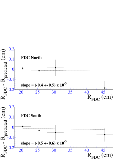
FIG. 16.: Residue of the radial position of the FDC track centroid from the predicted radial position of forward muon tracks at the FDC, as a function of the track radial position. The solid line is a fitted straight line constrained to pass through the origin.

We calibrate the shower centroid algorithm using Monte Carlo electrons simulated using geant and electrons from the $Z\to ee$ data. We apply a polynomial correction as a function of $r_{\rm cal}$ and the distance from the cell edges based on the Monte Carlo electrons. We refine the calibration with the $Z\to ee$ data by exploiting the fact that both electrons originate from the same vertex. Using the algorithm described in Sec. IV B 1, we determine a vertex for each electron from the shower centroid and the track coordinates. We minimize the difference between the two vertex positions as a function of an $r_{\rm cal}$ scale factor $\beta_{\rm EC}$ (see Fig. 17). The correction factor is $\beta_{\rm EC}=0.9997\pm 0.00044$ for EC North, and $\beta_{\rm EC}=1.00225\pm 0.00044$ for EC South. We find no systematic radial dependence of these correction factors.

We quantify the FDC and EC radial calibration uncertainty in terms of scale factor uncertainties $\delta\beta_{\rm FDC}=\pm 0.00054$ and $\delta\beta_{\rm EC}=\pm 0.0003$ for the radial coordinate. The uncertainties in these scale factors lead to a 20 MeV uncertainty in the EC $W$ boson mass measurement.

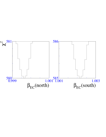
FIG. 17.: The $\chi^{2}$ versus $\beta_{\rm EC}$ value.

B Angular Resolutions

The resolution for the radial coordinate of the track, $r_{\rm trk}$, is determined from the $Z\to ee$ sample. Both electrons originate from the same interaction vertex and therefore the difference between the interaction vertices reconstructed from the two electrons separately, $z_{\rm vtx}(e_{1})-z_{\rm vtx}(e_{2})$, is a measure of the resolution with which the electrons point back to the vertex. The points in Fig. 18 show the distribution of $z_{\rm vtx}(e_{1})-z_{\rm vtx}(e_{2})$ observed in the CC/EC and EC/EC $Z$ samples with matching tracks required for both electrons.

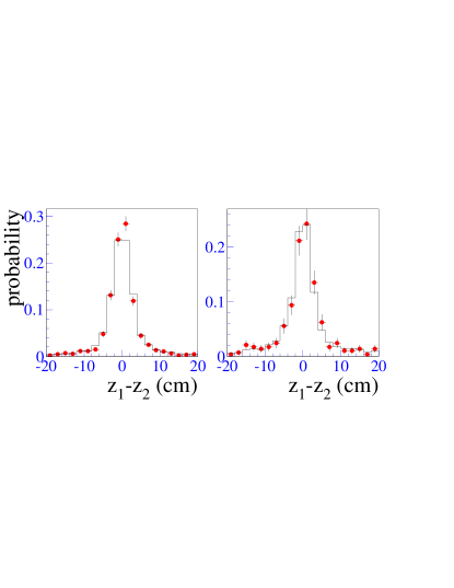
FIG. 18.: The distribution of $z_{\rm vtx}(e_{1})-z_{\rm vtx}(e_{2})$ for the CC/EC (left) and EC/EC (right) $Z\to ee$ samples ($\bullet$) and the fast Monte Carlo simulation (——).

A Monte Carlo study based on single electrons generated with a geant simulation shows that the resolution of the shower centroid algorithm is 0.1 cm in the EC, consistent with EC electron beam tests. We then tune the resolution function for $r_{\rm trk}$ in the fast Monte Carlo so that it reproduces the shape of the $z_{\rm vtx}(e_{1})-z_{\rm vtx}(e_{2})$ distribution observed in the data. We find that a resolution function consisting of two Gaussians 0.2 cm and 1.7 cm wide, with 20% of the area under the wider Gaussian, fits the data well. The histogram in Fig. 18 shows the Monte Carlo prediction for the best fit, normalized to the same number of events as the data.

C Underlying Event Energy

We define a cone which is projective from the center of the detector, has a radius of 20 cm at the $z$ position of ECEM3 and is centered on the electron cluster centroid. The cone extends over the four ECEM layers and the first ECFH layer. This cone contains the entire energy deposited by the electron shower plus some energy from other particles. The energy in the window is excluded from the computation of $\vec{u}_{T}$. This causes a bias in $u_{\parallel}$, the component of $\vec{u}_{T}$ along the direction of the electron. We call this bias $\Delta u_{\parallel}$. It is equal to the momentum flow observed in the EM and first FH sections of a projective cone of radius 20 cm at ECEM3.

We use the $W$ data sample to measure $\Delta u_{\parallel}$. For every electron in the $W$ sample, we compute the energy flow into an azimuthally rotated position, keeping the cone radius and the radial position the same. For the rotated position we compute the measured transverse energy. Since the $\eta\phi$ area of the cone increases as the electron $\eta$ increases, it is convenient to parameterize the transverse energy density, $\Delta u_{\parallel}$/$\delta\eta\delta\phi$.

At higher luminosity the average number of interactions per event increases and therefore $\Delta u_{\parallel}$/$\delta\eta\delta\phi$ increases (Fig. 20). The mean value of $\Delta u_{\parallel}$/$\delta\eta\delta\phi$ increases by 40 MeV per 10³⁰cm^-2s^-1. The underlying event energy flow into the electron cone depends on the electron $\eta$, as shown in Fig. 20, corrected back to zero luminosity.

The underlying event energy flow into the electron cone also depends on the overlap between the recoil and the electron. We have found that the best measure of the recoil overlap is the component of the total recoil in the direction of the electron, which is $u_{\parallel}$. Figure 21 shows $\langle\Delta u_{\parallel}/\delta\eta\delta\phi({\cal L}=0,\mid\!\eta\!\mid=2.0)\rangle$, the mean value for $\Delta u_{\parallel}$/$\delta\eta\delta\phi$ corrected to zero luminosity and $\mid\!\eta\!\mid=2.0$, as a function of $u_{\parallel}$. In the fast Monte Carlo model, a value $\Delta u_{\parallel}$/$\delta\eta\delta\phi$ is picked from the distribution shown in Fig. 22 for every event, corrected for $u_{\parallel}$, $\eta$, and luminosity dependences, and then scaled by the $\delta\eta\delta\phi$ area of a 20 cm cone at the electron $\eta$.

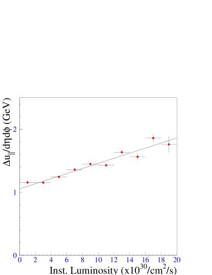
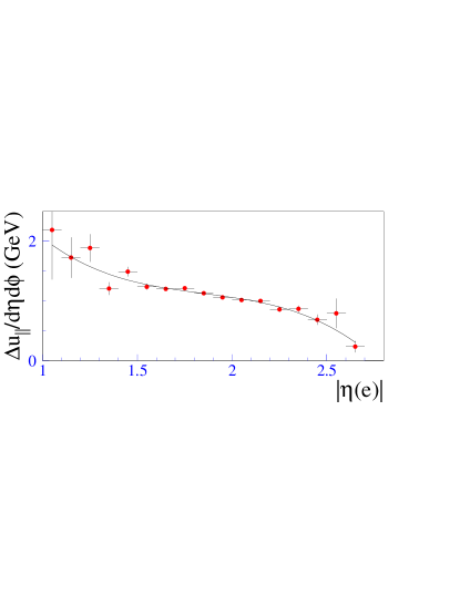
FIG. 19.: The instantaneous luminosity dependence of $\langle\Delta u_{\parallel}/\delta\eta\delta\phi\rangle$.

FIG. 20.: The variation of $\langle\Delta u_{\parallel}/\delta\eta\delta\phi\rangle$ as a function of electron $\eta$.

FIG. 21.: The variation of $\langle\Delta u_{\parallel}/\delta\eta\delta\phi\rangle$ as a function of $u_{\parallel}$. The region between the arrows is populated by the $W$ boson sample.

FIG. 22.: The distribution of $\Delta u_{\parallel}$/$\delta\eta\delta\phi$ in the $W$ signal sample, corrected to $\cal L$=0, $\mid\!\eta\!\mid=2$, $u_{\parallel}$=0 .

The measured electron transverse energy is biased upwards by the additional energy $\Delta E_{T}$ in the window from the underlying event. $\Delta E_{T}$ is not equal to $\Delta u_{\parallel}$ because the electron $E_{T}$ is calculated by scaling the sum of the cell energies by the electron angle, whereas $u_{T}$ is obtained by summing the $E_{T}$ of each cell. The ratio of the two corrections as a function of electron $\eta$ is shown in Fig. 23.

FIG. 23.: The ratio of the $\langle\Delta u_{\parallel}/\delta\eta\delta\phi\rangle$ corrections to the electron and the recoil as a function of electron $\eta$.

The uncertainty in the underlying event transverse energy density has a statistical component (14 MeV) and a systematic component (24 MeV). The systematic component is derived from the difference between the measurement close to the electron (where it is biased by the isolation requirement) and far from the electron (where it is not biased). The total uncertainty in the underlying event transverse energy density is 28 MeV.

D $u_{\parallel}$ Efficiency

The efficiency for electron identification depends on the electron environment. Well-isolated electrons are identified correctly more often than electrons near other particles. Therefore $W$ decays in which the electron is emitted in the same direction as the particles recoiling against the $W$ boson are selected less often than $W$ decays in which the electron is emitted in the direction opposite the recoiling particles. This causes a bias in the lepton $p_{T}$ distributions, shifting $p_{T}(e)$ to larger values and $p_{T}(\nu)$ to lower values, whereas the $m_{T}$ distribution is only slightly affected.

We measure the electron finding efficiency as a function of $u_{\parallel}$ using $Z\rightarrow ee$ events. The $Z$ event is tagged with one electron, and the other electron provides an unbiased measurement of the efficiency. Following background subtraction, the measured efficiency is shown in Fig. 24. The line is a fit to a function of the form

$$\varepsilon(u_{\parallel})=\varepsilon_{0}\left\{\begin{array}[]{ll}1&\hbox{for $u_{\parallel}<u_{0}$}\\ 1-s(u_{\parallel}-u_{0})&\hbox{otherwise.}\end{array}\right.$$ (37)

The parameter $\varepsilon_{0}$ is an overall efficiency which is inconsequential for the $W$ mass measurement, $u_{0}$ is the value of $u_{\parallel}$ at which the efficiency starts to decrease as a function of $u_{\parallel}$, and $s$ is the rate of decrease. We obtain the best fit for $u_{0}=-2.4$ GeV and $s=0.0029$ GeV^-1. These two values are strongly anti-correlated. The error on the slope $\delta s=\pm 0.0012$ GeV^-1 accounts for the statistics of the $Z$ sample.

FIG. 24.: The EC electron selection efficiency as a function of $u_{\parallel}$.

E Electron Energy Response

Equation 6 relates the reconstructed electron energy to the recorded end calorimeter signals. Since the values for the constants were determined in the test beam, we determine the offset $\delta_{\rm EC}$ and a scale $\alpha_{\rm EC}$, which essentially modifies $A$, in situ with collider $Z\rightarrow ee$ data.

The electrons from $Z$ decays are not monoenergetic and therefore we can make use of their energy spread to constrain $\delta_{\rm EC}$. When both electrons are in the EC, we can write

$$m(ee)=\alpha_{\rm EC}M_{Z}+f_{Z}\delta_{\rm EC}\$$ (38)

for $\delta_{\rm EC}\ll E(e_{1})+E(e_{2})$. $f_{Z}$ is a kinematic function related to the boost of the $Z$ boson, and is given by $f_{Z}=[E(e_{1})+E(e_{2})](1-\cos\omega)/m(ee)$, where $\omega$ is the opening angle between the two electrons. When one electron is in the CC and one is in the EC, we can write

$$m(ee)=\sqrt{\alpha_{\rm CC}\alpha_{\rm EC}}M_{Z}+f_{Z}\delta_{\rm EC},$$ (39)

where $f_{Z}=E(e_{2})(1-\cos\omega)/m(ee)$ and $e_{2}$ is the CC electron. When we apply this formula, we have already corrected the CC electron for the corresponding CCEM offset, $\delta_{\rm CC}$ = $-0.16$ GeV, which was measured for our CC $W$ mass analysis [4]. $\alpha_{\rm CC}$ is the CC electromagnetic energy scale, which is determined by fitting the $m(ee)$ spectrum of the CC/CC $Z$ sample.

We plot $m(ee)$ versus $f_{Z}$ and extract $\delta_{\rm EC}$ as the slope of the fitted straight line. We use the fast Monte Carlo to correct for residual biases introduced by the kinematic cuts. The $\delta_{\rm EC}$ measurements from the CC/EC and EC/EC $Z$ samples are shown in Fig. 25 along with the statistical uncertainties. We obtain the average $\delta_{\rm EC}=-0.1\pm 0.7$ GeV. The uncertainty in this measurement of $\delta_{\rm EC}$ is dominated by the statistical uncertainty due to the finite size of the $Z$ sample. As Fig. 25 shows, the offsets measured in the north and south end calorimeters separately are completely consistent.

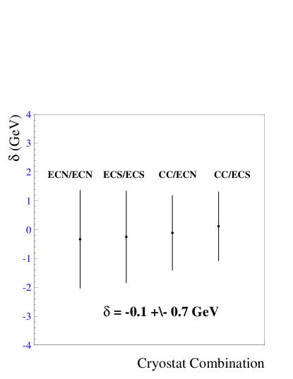
FIG. 25.: The ECEM offset measurements using the CC/EC and EC/EC $Z$ samples. The labels indicate the calorimeter cryostat in which each of the $Z$ decay electrons was detected. CC indicated the central calorimeter and ECN (ECS) indicates the north (south) end calorimeter respectively.

After correcting the data with this value of $\delta_{\rm EC}$ we determine $\alpha_{\rm EC}$ so that the position of the $Z$ peak predicted by the fast Monte Carlo agrees with the data. To determine the scale factor that best fits the data, we perform a maximum likelihood fit to the $m(ee)$ spectrum between 70 GeV and 110 GeV. In the resolution function we allow for background shapes determined from samples of events with two EM clusters that fail the electron quality cuts (Fig. 26). The background normalization is obtained from the sidebands of the $Z$ peak.

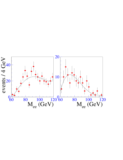
FIG. 26.: The dielectron mass spectrum from the CC/EC (left) and EC/EC (right) samples of events with two EM clusters that fail the electron quality cuts. The superimposed curves shows the fitted functions used to model the shape of the background in the $Z$ samples.

Figure 27 shows the $m(ee)$ spectrum for the CC/EC $Z$ sample and the Monte Carlo spectrum that best fits the data for $\delta_{\rm EC}=-0.1$ GeV. The $\chi^{2}$ for the best fit to the CC/EC $m(ee)$ spectrum is 14 for 19 degrees of freedom. For $\alpha_{\rm EC}=0.95143\pm 0.00259$, the $Z$ peak position of the CC/EC sample is consistent with the known $Z$ boson mass. The error reflects the statistical uncertainty. The background has no measurable effect on the result.

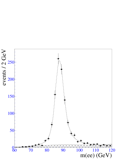
FIG. 27.: The dielectron mass spectrum from the CC/EC $Z$ sample. The superimposed curve shows the maximum likelihood fit and the shaded region the fitted background.

Figure 28 shows the $m(ee)$ spectrum for the EC/EC $Z$ sample and the Monte Carlo spectrum that best fits the data for $\delta_{\rm EC}=-0.1$ GeV. The $\chi^{2}$ for the best fit to the EC/EC $m(ee)$ spectrum is 12 for 17 degrees of freedom. For $\alpha_{\rm EC}=0.95230\pm 0.00231$, the $Z$ peak position of the EC/EC sample is consistent with the known $Z$ boson mass. The error reflects the statistical uncertainty and the uncertainty in the background.

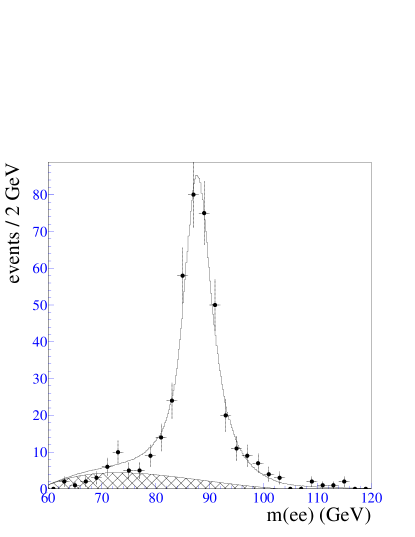
FIG. 28.: The dielectron mass spectrum from the EC/EC $Z$ sample. The superimposed curve shows the maximum likelihood fit and the shaded region the fitted background.

Combining the $\alpha_{\rm EC}$ measurements from the CC/EC and the EC/EC $Z$ samples, we obtain the ECEM energy scale

$$\alpha_{\rm EC}=0.95179\pm 0.00187\quad.$$ (40)

The difference between the ECEM scales measured separately in the north and south calorimeters is $0.0040\pm 0.0037$, consistent with the calorimeters having the same EM response.

F Electron Energy Resolution

Equation 8 gives the functional form of the electron energy resolution. We take the intrinsic resolution of the end calorimeter, which is given by the sampling term $s_{\rm EM}$, from the test beam measurements. The noise term $n_{\rm EM}$ is represented by the width of the electron underlying event energy distribution (Fig. 22). We measure the constant term $c_{\rm EM}$ from the $Z$ line shape of the data. We fit a Breit-Wigner convoluted with a Gaussian, whose width characterizes the dielectron mass resolution, to the $Z$ peaks for the CC/EC and EC/EC samples separately. Figure 29 shows the width $\sigma_{m(ee)}$ of the Gaussian fitted to the $Z$ peak predicted by the fast Monte Carlo as a function of $c_{\rm EM}$. The horizontal lines indicate the width of the Gaussian fitted to the $Z$ samples and its uncertainties. For the data measurements of

$$\sigma_{m}=2.47\;\pm\;0.05\;{\rm GeV}\;{\rm(CC/EC)}$$ (41)

$$\sigma_{m}=2.72\;\pm\;0.11\;{\rm GeV}\;{\rm(EC/EC)}$$ (42)

we extract from the CC/EC $Z$ boson events $c_{\rm EC}=1.6^{+0.8}_{-1.6}$% and from the EC/EC $Z$ events we extract $c_{\rm EC}=0.0^{+1.0}_{-0.0}$%. We take the combined measurement to be

$$c_{\rm EC}=1.0^{+0.6}_{-1.0}\;{\rm\%}.$$ (43)

The measured $Z$ boson mass does not depend on $c_{\rm EC}$.

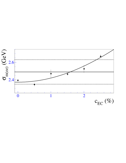
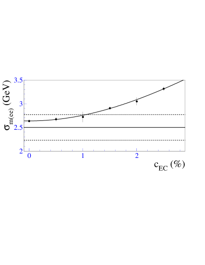
FIG. 29.: The dielectron mass resolution versus the constant term $c_{\rm EM}$. The top plot is for the CC/EC $Z$ events and the bottom plot is for the EC/EC $Z$ events.

VII Recoil Measurement

A Recoil Momentum Response

The detector response and resolution for particles recoiling against a $W$ boson should be the same as for particles recoiling against a $Z$ boson. For $Z\to ee$ events, we can measure the transverse momentum of the $Z$ boson from the $e^{+}e^{-}$ pair, $p_{T}(ee)$, into which it decays, and from the recoil momentum $u_{T}$ in the same way as for $W\to e\nu$ events. By comparing $p_{T}(ee)$ and $u_{T}$, we calibrate the recoil response relative to the electron response.

The recoil momentum is carried by many particles, mostly hadrons, with a wide momentum spectrum. Since the response of the calorimeter to hadrons is slightly nonlinear at low energies, and the recoil particles see a reduced response at module boundaries, we expect a momentum-dependent response function with values below unity. To fix the functional form of the recoil momentum response, we studied [4] the response predicted by a Monte Carlo $Z\to ee$ sample obtained using the herwig program and a geant-based detector simulation. We projected the reconstructed transverse recoil momentum onto the transverse direction of motion of the $Z$ boson and define the response as

$${\rm R_{rec}}=\frac{\left|\vec{u}_{T}\cdot\hat{q}_{T}\right|}{\left|q_{T}\right|},$$ (44)

where $q_{T}$ is the generated transverse momentum of the $Z$ boson. A response function of the form

$${\rm R_{rec}}=\alpha_{\rm rec}+\beta_{\rm rec}\ln\left(q_{T}/\hbox{GeV}\right)$$ (45)

fits the response predicted by geant with $\alpha_{\rm rec}=0.713\pm 0.006$ and $\beta_{\rm rec}=0.046\pm 0.002$. This functional form also describes the jet energy response [42] of the DØ calorimeter.

The recoil response for data was calibrated against the electron response by requiring $p_{T}$ balance in $Z\rightarrow ee$ decays for our published CC analysis [4]. The $Z$ boson $p_{T}$ measured with the electrons and the recoil are projected on the $\eta$ axis, defined as the bisector of the two electron directions in the transverse plane. From the CC/CC + CC/EC $Z$ boson events, we measured $\alpha_{\rm rec}=0.693\pm 0.060$ and $\beta_{\rm rec}=0.040\pm 0.021$, in good agreement with the Monte Carlo prediction. To compare the recoil response measured with $Z$ events of different topologies, we scale the recoil measurement with the inverse of the response parametrization

$$R_{\rm rec}=0.693\;+\;0.04\cdot\ln\;(p_{T}(ee)/{\rm GeV})$$ (46)

and plot the sum of the projections versus $p_{\eta}(ee)$, as shown in Fig. 30. We see no $p_{\eta}(ee)$ dependence to the $p_{\eta}$ balance measured using the $Z$ boson events with at least one central electron, since this sample was used to derive the values of these parameters. The EC/EC $Z$ boson events give a recoil response measurement statistically consistent with the above. Hence we use the same recoil response for the EC and the CC $W$ boson events [4].

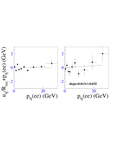
FIG. 30.: The recoil momentum response in the CC/CC + CC/EC (left) and the EC/EC (right) $Z$ samples as a function of $p_{\eta}(ee)$.

B Recoil Momentum Resolution

The widths of the $p_{\eta}$ balance and the $p_{\xi}$ balance (where the $\xi$ axis is perpendicular to the $\eta$ axis) are sensitive to the recoil resolution. Figures 31–32 show the comparison between the data and Monte Carlo for the recoil resolution determined in our CC $W$ mass analysis [4]. The $p_{\eta}$ balance width is in good agreement between data and Monte Carlo for all $Z$ boson topologies. Hence we use the same recoil resolution for EC $W$ boson events as for the CC $W$ boson events [4].

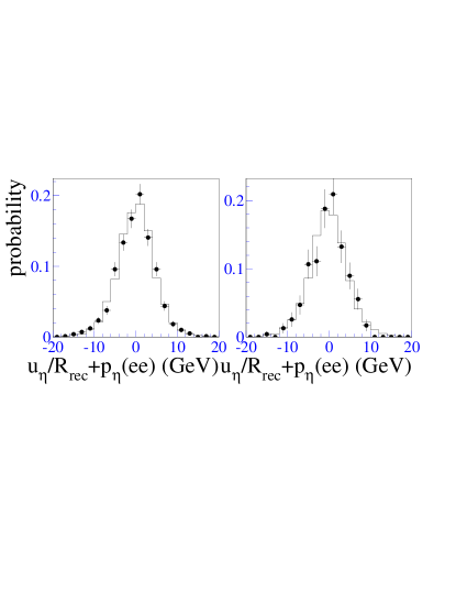
FIG. 31.: The $\eta$-balance distribution for the $Z$ boson data ($\bullet$) and the fast Monte Carlo simulation (—–). The plot on the left is for the CC/CC + CC/EC $Z$ events and the plot on the right is for the EC/EC $Z$ events.

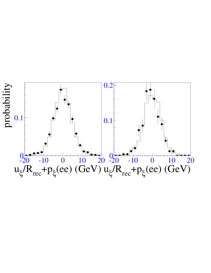
FIG. 32.: The $\xi$-balance distribution for the $Z$ boson data ($\bullet$) and the fast Monte Carlo simulation (—–). The plot on the left is for the CC/CC + CC/EC $Z$ events and the plot on the right is for the EC/EC $Z$ events.

C Comparison with $W$ Boson Data

We compare the recoil momentum distributions in the $W$ boson data to the predictions of the fast Monte Carlo, which includes the parameters described in this section and Sec. VI. Figure 33 shows the $u_{\parallel}$ spectra from Monte Carlo and $W$ data. The agreement means that the recoil momentum response and resolution and the $u_{\parallel}$ efficiency parameterization describe the data well. Figures 34–36 show $u_{\perp}$, $u_{T}$, and the azimuthal difference between electron and recoil directions from Monte Carlo and $W$ boson data. The figures also show the mean and r.m.s. of the data and Monte Carlo distributions and the $\chi^{2}$ over the number of degrees of freedom (dof).

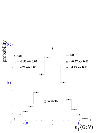
FIG. 33.: The $u_{\parallel}$ spectrum for the $W$ data ($\bullet$) and the Monte Carlo simulation (—–). The mean ($\mu$) and r.m.s. ($\sigma$) of the distributions and the $\chi^{2}$/dof is also shown.

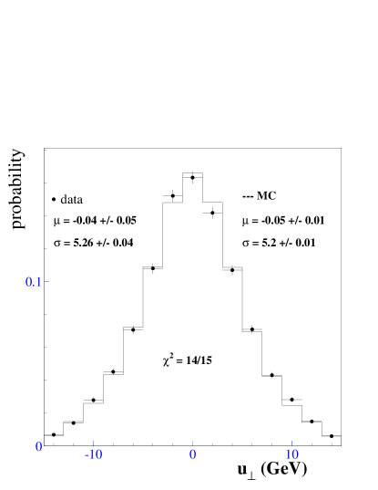
FIG. 34.: The $u_{\perp}$ spectrum for the $W$ data ($\bullet$) and the Monte Carlo simulation (—–). The mean ($\mu$) and r.m.s. ($\sigma$) of the distributions and the $\chi^{2}$/dof is also shown.

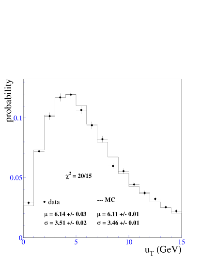
FIG. 35.: The recoil momentum ($u_{T}$) spectrum for the $W$ data ($\bullet$) and the Monte Carlo simulation (—–). The mean ($\mu$) and r.m.s. ($\sigma$) of the distributions and the $\chi^{2}$/dof is also shown.

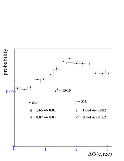
FIG. 36.: The azimuthal difference between electron and recoil directions for the $W$ data ($\bullet$) and the Monte Carlo simulation (—–). The mean ($\mu$) and r.m.s. ($\sigma$) of the distributions and the $\chi^{2}$/dof is also shown.

VIII Constraints on the $W$ Boson Rapidity Spectrum

In principle, if the acceptance for the $W\rightarrow e\nu$ decays were complete, the transverse mass distribution or the lepton $p_{T}$ distributions would be independent of the $W$ rapidity. However, cuts on the electron angle in the laboratory frame cause the observed distributions of the transverse momenta to depend on the $W$ rapidity. Hence a constraint on the $W$ rapidity distribution is useful in constraining the production model uncertainty on the $W$ mass.

The pseudorapidity distribution of the electron from $W\rightarrow e\nu$ decays is correlated with the rapidity distribution of the $W$ boson. Therefore we can compare the electron $\eta$ distribution between data and Monte Carlo.

To compare the data with the Monte Carlo, we need to correct for the jet background in the data and the electron identification efficiency as a function of $\eta$. We obtain the jet background fraction as a function of $\eta$ by counting the number of $W$ events that fail electron cuts (see Sec. IX B) in bins of $\eta$, subtracting the small contamination due to true electrons, and normalizing the entire distribution to the total background fraction (separately in the CC and EC). The normalized background $\eta$ distribution is subtracted from the $\eta$ distribution of the data.

The electron identification efficiency (after fiducial and kinematic cuts) is measured using the CC/CC and CC/EC $Z\rightarrow ee$ events. All the electron identification cuts are used to identify one electron to tag the event. Candidates are selected in the mass range $81<m_{ee}<101$ GeV. Sidebands in the mass range $60<m_{ee}<70$ GeV and $110<m_{ee}<120$ GeV are used for background subtraction. The number of events in which the second electron also satisfies all the electron identification cuts is used to calculate the efficiency. The efficiency measured in bins of the $\eta$ of the second electron is shown in Fig. 37.

FIG. 37.: Dependence of electron identification efficiency on electron pseudorapidity. Statistical errors are shown.

We scale the electron $\eta$ distribution predicted by the Monte Carlo by the $\eta$-dependent efficiency, and compare to the background-subtracted data in Fig. 38. The errors on the Monte Carlo points include the statistical errors on the Monte Carlo sample and the statistical errors on the efficiency measurements. The errors on the data points include the statistical errors on the number of candidate events and the statistical errors on the background estimate which has been subtracted. Figure 39 shows the ratio between the background-subtracted data and the efficiency-corrected Monte Carlo, with the uncertainties mentioned above added in quadrature. The Monte Carlo has been normalized to the data. The $\chi^{2}$/dof shown is with respect to unity. There is good agreement between the data and the Monte Carlo.

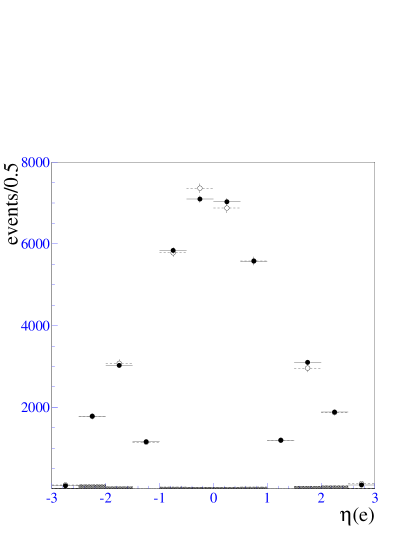
FIG. 38.: $\eta$ distribution of the electron from $W\rightarrow e\nu$ decays from background-subtracted data ($\bullet$), efficiency-corrected Monte Carlo ($\circ$) and the jet background (shaded histogram). The distributions drop near $\mid\!\eta\!\mid=1.2$ because there is no EM calorimetry in the range $1.1<\mid\!\eta_{\rm det}\!\mid<1.4$.

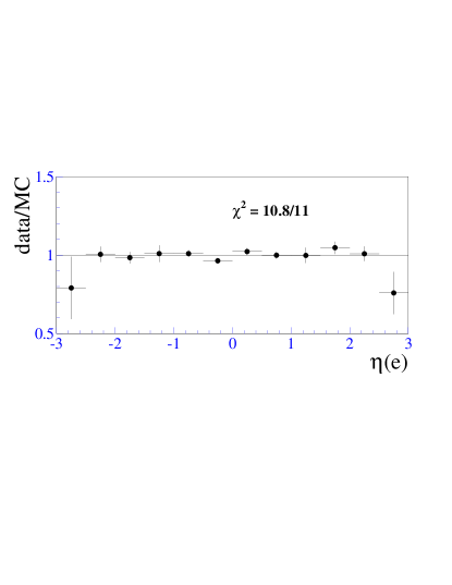
FIG. 39.: The ratio of the background-subtracted data and efficiency-corrected Monte Carlo. The Monte Carlo has been normalized to the data. The $\chi^{2}$/dof is with respect to unity.

To extract a constraint on the $y$ distribution of the $W$ boson, we introduce in the Monte Carlo a scale factor as follows:

$$y_{W}\rightarrow k_{\eta}\cdot y_{W}$$ (47)

i.e. the rapidity of the $W$ is scaled by the factor $k_{\eta}$. We then compute the $\chi^{2}$ between the data and Monte Carlo $\eta(e)$ distributions for different $k_{\eta}$. The result is shown in Fig. 40 for the MRS(A^′) [43] parton distribution functions. Table IV shows the values of $k_{\eta}$ at which the $\chi^{2}$ is minimized for the different pdf’s.

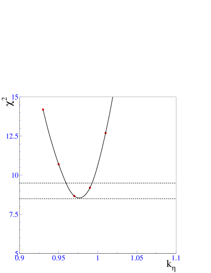
FIG. 40.: $\chi^{2}$ of the electron $\eta$ distribution ratio between data and Monte Carlo from unity, as a function of the $W$ rapidity scale factor $k_{\eta}$. There are 11 degrees of freedom. The Monte Carlo uses the MRS(A^′) parton distribution functions. The horizontal lines indicate $\chi^{2}_{\rm min}$ and $\chi^{2}_{\rm min}+1$.

The uncertainty in $k_{\eta}$ is 1.6%, which is the change in $k_{\eta}$ that causes the $\chi^{2}$ to rise by one unit above the minimum. We generate Monte Carlo events with different values of $k_{\eta}$ and fit them with templates generated with $k_{\eta}$ set to unity. For a $k_{\eta}$ variation of 1.6%, the variation of the fitted $W$ mass in the EC is shown in Table V.

TABLE IV.: Value of $k_{\eta}$ giving the minimum $\chi^{2}$ for different pdf’s.

MRS(A′) [43]	CTEQ3M [44]	CTEQ2M [45]	MRSD$-^{\prime}$ [46]
0.975	0.98	0.985	0.99

TABLE V.: Variation in fitted EC $W$ mass due to a 1.6% variation in $k_{\eta}$.

	$m_{T}$ fit	$p_{T}(e)$ fit	$p_{T}(\nu)$ fit
$\delta M_{W}$ (MeV)	34	48	25

The comparison of the electron $\eta$ distribution between the data and the Monte Carlo provides a consistency check of the predicted $W$ rapidity distribution, and hence of the pdf’s. The measured $k_{\eta}$ being consistent with unity sets an upper bound on the pdf uncertainty. While this constraint can potentially be much more powerful with higher statistics obtained in future data-taking, it is presently weaker than the uncertainty in the modern pdf’s. Therefore we do not use this constraint to set our final $W$ mass uncertainty due to pdf’s. However, since our data used for this constraint are independent of the world data used to derive the pdf’s, we have additional evidence that the uncertainty on the $W$ mass due to the pdf’s is not being underestimated.

IX Backgrounds

A $W\to\tau\nu\to e\nu\overline{\nu}\nu$

The decay $W\to\tau\nu\to e\nu\overline{\nu}\nu$ is topologically indistinguishable from $W\to e\nu$. It is included in the fast Monte Carlo simulation (Sec. V). This decay is suppressed by the branching fraction for $\tau\to e\nu\overline{\nu}$ $\left(17.83\pm 0.08\right)$% [19], and by the lepton $p_{T}$ cuts. It accounts for 1% of the events in the $W$ sample.

B Hadronic Background

QCD processes can fake the signature of a $W\to e\nu$ decay if a hadronic jet fakes the electron signature and the transverse momentum balance is mismeasured.

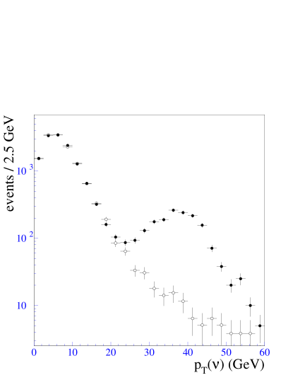
FIG. 41.: The $\hbox to0.0pt{\kern 1.00006pt/\hss}p_{T}$ spectra of a sample of events passing electron identification cuts ($\bullet$) and a sample of events failing the cuts ($\circ$).

We estimate this background from the $\hbox to0.0pt{\kern 1.00006pt/\hss}p_{T}$ spectrum of data events with an electromagnetic cluster. Electromagnetic clusters in events with low $\hbox to0.0pt{\kern 1.00006pt/\hss}p_{T}$ are almost all due to jets. Some of these clusters satisfy our electron selection criteria and fake an electron. From the shape of the $\hbox to0.0pt{\kern 1.00006pt/\hss}p_{T}$ spectrum for these events we determine how likely it is for these events to have sufficient $\hbox to0.0pt{\kern 1.00006pt/\hss}p_{T}$ to enter our $W$ sample.

We determine this shape by selecting isolated electromagnetic clusters that have $\chi^{2}>200$ and the 4-variable likelihood $\lambda_{4}>30$. Nearly all electrons fail this cut, so that the remaining sample consists almost entirely of hadrons. We use data collected using a trigger without the $\hbox to0.0pt{\kern 1.00006pt/\hss}p_{T}$ requirement to study the efficiency of this cut for jets. If we normalize the background spectrum after correcting for residual electrons to the electron sample, we obtain an estimate of the hadronic background in an electron candidate sample. Figure 41 shows the $\hbox to0.0pt{\kern 1.00006pt/\hss}p_{T}$ spectra of both samples, normalized for $\mbox{$\hbox to0.0pt{\kern 1.00006pt/\hss}p_{T}$}<10$ GeV. We find the hadronic background fraction of the total $W$ sample after all cuts to be $f_{\rm had}=\left(3.64\pm 0.78\right)$%. The error receives contributions from the uncertainty in the relative normalization of the two samples at low $\hbox to0.0pt{\kern 1.00006pt/\hss}p_{T}$, the statistics of the failed electron sample, and the uncertainty in the residual contamination of the failed electron sample by true electrons. We fit the distributions of the background events with $\mbox{$\hbox to0.0pt{\kern 1.00006pt/\hss}p_{T}$}>30$ GeV to estimate the shape of the background contributions to the $p_{T}(e)$, $p_{T}(\nu)$, and $m_{T}$ spectra (Fig. 42). We use the statistical error of the fits to estimate the uncertainty in the background shapes.

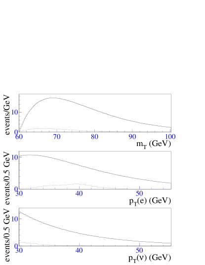
FIG. 42.: Shapes of $m_{T}$, $p_{T}(e)$, and $p_{T}(\nu)$ spectra from hadron (——) and $Z$ boson (- - -) backgrounds with the proper relative normalization.

C $Z\to ee$

To estimate the fraction of $Z\to ee$ events that satisfy the $W$ boson event selection, we use a Monte Carlo sample of approximately 100,000 $Z\to ee$ events generated with the herwig program and a detector simulation based on geant. The boson $p_{T}$ spectrum generated by herwig agrees reasonably well with the calculation in Ref. [29] and with our $Z$ boson $p_{T}$ measurement [50]. $Z\to ee$ decays typically enter the $W$ sample when one electron satisfies the $W$ cuts and the second electron is lost or mismeasured, causing the event to have large $\hbox to0.0pt{\kern 1.00006pt/\hss}p_{T}$.

An electron is most frequently mismeasured when it goes into the regions between the CC and one of the ECs, which are covered only by the hadronic section of the calorimeter. These electrons therefore cannot be identified, and their energy is measured in the hadronic calorimeter. Large $\hbox to0.0pt{\kern 1.00006pt/\hss}p_{T}$ is more likely for these events than when both electrons hit the EM calorimeters.

We make the $W$ and $Z$ selection cuts on the Monte Carlo events, and normalize the number of events passing the $W$ cuts to the number of $W$ data events, scaled by the ratio of selected $Z$ data and Monte Carlo events. We estimate the fraction of $Z$ events in the $W$ sample to be $f_{Z}=\left(0.26\pm 0.02\right)\%$. The uncertainties quoted include systematic uncertainties in the matching of momentum scales between Monte Carlo and collider data. Figure 42 shows the distributions of $p_{T}(e)$, $p_{T}(\nu)$, and $m_{T}$ for the $Z$ events with one lost or mismeasured electron that satisfy the $W$ selection.

X Mass Fits

A Maximum Likelihood Fitting Procedure

We use a binned maximum likelihood fit to extract the $W$ mass. Using the fast Monte Carlo program, we compute the $m_{T}$, $p_{T}(e)$, and $p_{T}(\nu)$ spectra for 200 hypothesized values of the $W$ mass between 79.7 and 81.7 GeV. For the spectra we use 250 MeV bins. The statistical precision of the spectra for the $W$ mass fit corresponds to about 8 million $W$ decays. When fitting the collider data spectra, we add the background contributions with the shapes and normalizations described in Sec. IX to the signal spectra. We normalize the spectra within the fit interval and interpret them as probability density functions to compute the likelihood

$$L(m)=\prod_{i=1}^{N}p_{i}^{n_{i}}(m),$$ (48)

where $p_{i}(m)$ is the probability density for bin $i$, assuming $M_{W}=m$, and $n_{i}$ is the number of data entries in bin $i$. The product runs over all $N$ bins inside the fit interval. We fit $-\ln[L(m)]$ with a quadratic function of $m$. The value of $m$ at which the function assumes its minimum is the fitted value of the $W$ mass and the 68% confidence level interval is the interval in $m$ for which $-\ln[L(m)]$ is within half a unit of its minimum.

B Electron $p_{T}$ Spectrum

We fit the $p_{T}(e)$ spectrum in the region $32<p_{T}(e)<50$ GeV. The interval is chosen to span the Jacobian peak. The data points in Fig. 43 represent the $p_{T}(e)$ spectrum from the $W$ sample. The solid line shows the sum of the simulated $W$ signal and the estimated background for the best fit, and the shaded region indicates the sum of the estimated hadronic and $Z\to ee$ backgrounds. The maximum likelihood fit gives

$$M_{W}=80.547\pm 0.128\ \hbox{GeV}$$ (49)

for the $W$ mass. Figure 44 shows $-\ln(L(m)/L_{0})$ for this fit, where $L_{0}$ is an arbitrary number.

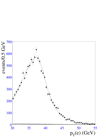
FIG. 43.: Spectrum of $p_{T}(e)$ from the $W$ data. The superimposed curve shows the maximum likelihood fit and the shaded region the estimated background.

FIG. 44.: The likelihood function for the $p_{T}(e)$ fit.

As a goodness-of-fit test, we divide the fit interval into 0.5 GeV bins, normalize the integral of the probability density function to the number of events in the fit interval, and compute $\chi^{2}=\sum_{i=1}^{N}(y_{i}-P_{i})^{2}/y_{i}$. The sum runs over all $N$ bins, $y_{i}$ is the observed number of events in bin $i$, and $P_{i}$ is the integral of the normalized probability density function over bin $i$. The parent distribution is the $\chi^{2}$ distribution for $N-2$ degrees of freedom. For the spectrum in Fig. 43 we compute $\chi^{2}=46$. For 36 bins there is a 8% probability for $\chi^{2}\geq 46$. Figure 45 shows the contributions $\chi_{i}=(y_{i}-P_{i})/\sqrt{y_{i}}$ to $\chi^{2}$ for the 36 bins in the fit interval.

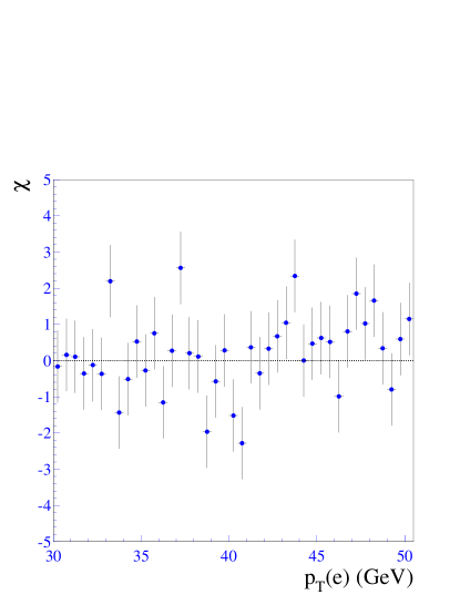
FIG. 45.: The $\chi$ distribution for the fit to the $p_{T}(e)$ spectrum.

Figure 46 shows the sensitivity of the fitted mass value to the choice of fit interval. The points in the two plots indicate the observed deviation of the fitted mass from the value given in Eq. 49. We expect some variation due to statistical fluctuations in the spectrum and systematic uncertainties in the probability density functions. We estimate the effect due to statistical fluctuations using Monte Carlo ensembles. We expect the fitted values to be inside the shaded regions indicated in the two plots with 68% probability. The dashed lines indicate the statistical error for the nominal fit. Figure 46 shows that the probability density function provides a good description of the observed spectrum.

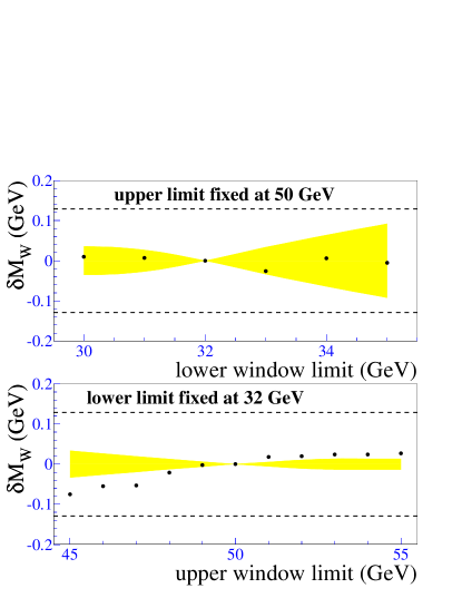
FIG. 46.: Variation of the fitted mass with the $p_{T}(e)$ fit window limits. See text for details.

C Transverse Mass Spectrum

The $m_{T}$ spectrum is shown in Fig. 47. The points are the observed spectrum, the solid line shows signal plus background for the best fit, and the shaded region indicates the estimated background contamination. We fit in the interval $65<m_{T}<90$ GeV. Figure 48 shows $-\ln(L(m)/L_{0})$ for this fit where $L_{0}$ is an arbitrary number. The best fit occurs for

$$M_{W}=80.757\pm 0.107\ \hbox{GeV}.$$ (50)

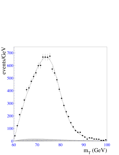
FIG. 47.: Spectrum of $m_{T}$ from the $W$ data. The superimposed curve shows the maximum likelihood fit and the shaded region shows the estimated background.

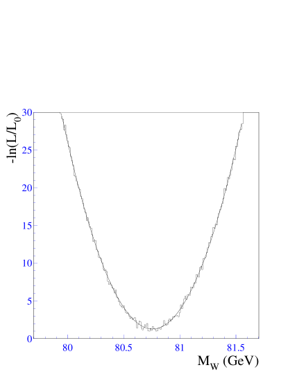
FIG. 48.: The likelihood function for the $m_{T}$ fit.

Figure 49 shows the deviations of the data from the fit. Summing over all bins in the fitting window, we get $\chi^{2}=17$ for 25 bins. For 25 bins there is a 81% probability to obtain a larger value. Figure 50 shows the sensitivity of the fitted mass to the choice of fit interval.

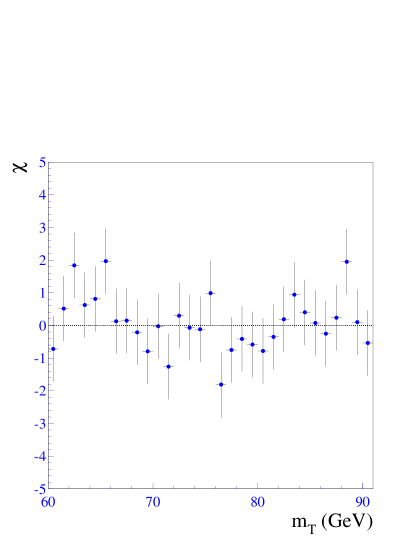
FIG. 49.: The $\chi$ distribution for the fit to the $m_{T}$ spectrum.

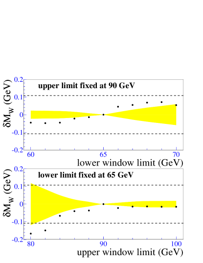
FIG. 50.: Variation of the fitted mass with the $m_{T}$ fit window limits. See text for details.

D Neutrino $p_{T}$ Spectrum

Figure 51 shows the neutrino $p_{T}$ spectrum. The points are the observed spectrum, the solid line shows signal plus background for the best fit, and the shaded region indicates the estimated background contamination. We fit in the interval $32<p_{T}(\nu)<50$ GeV. Figure 52 shows $-\ln(L(m)/L_{0})$ for this fit where $L_{0}$ is an arbitrary number. The best fit occurs for

$$M_{W}=80.740\pm 0.159\ \hbox{GeV}.$$ (51)

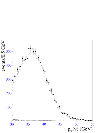
FIG. 51.: Spectrum of $p_{T}(\nu)$ from the $W$ data. The superimposed curve shows the maximum likelihood fit and the shaded region shows the estimated background.

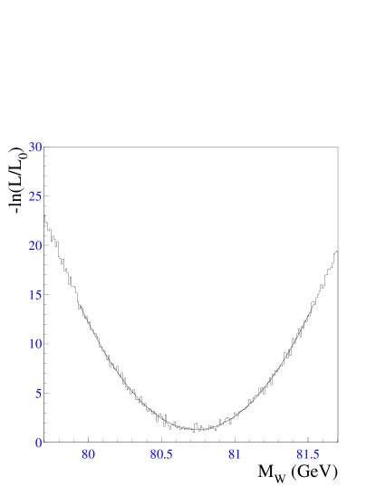
FIG. 52.: The likelihood function for the $p_{T}(\nu)$ fit.

Figure 53 shows the deviations of the data from the fit. Summing over all bins in the fitting window, we get $\chi^{2}=37$ for 36 bins. For 36 bins there is a 33% probability to obtain a larger value. Figure 54 shows the sensitivity of the fitted mass to the choice of fit interval.

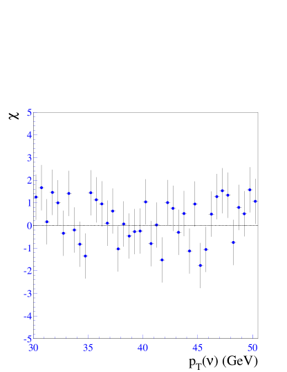
FIG. 53.: The $\chi$ distribution for the fit to the $p_{T}(\nu)$ spectrum.

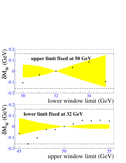
FIG. 54.: Variation of the fitted mass with the $p_{T}(\nu)$ fit window limits. See text for details.

XI Consistency Checks

A North vs South Calorimeters

Since the detector is north-south symmetric, we expect the measurements made with the north and south calorimeters separately to be consistent. We find

$$M_{W}^{\rm ECN}-M_{W}^{\rm ECS} = \>\;\;\;\;88\;\pm\;215\;{\rm MeV}\;(m_{T}\;{\rm fit)}$$ (52)

$$M_{W}^{\rm ECN}-M_{W}^{\rm ECS} = -116\;\pm\;258\;{\rm MeV}\;(p_{T}^{e}\;{\rm fit)}$$ (53)

$$M_{W}^{\rm ECN}-M_{W}^{\rm ECS} = \>\;\;107\;\pm\;318\;{\rm MeV}\;(p_{T}^{\nu}\;{\rm fit)}$$ (54)

where the uncertainty is statistical only.

B Time Dependence

We divide the $W$ boson data sample into five sequential calender time intervals such that the subsamples have equal number of events. We generate resolution functions for the luminosity distribution of these five subsamples. We fit the transverse mass and lepton $p_{T}$ spectra from the $W$ samples in each time bin. The fitted masses are plotted in Fig. 55 where the time bins are labelled by run blocks. The errors shown are statistical only. We compute the $\chi^{2}$ with respect to the $W$ mass fit to the entire data sample. The $\chi^{2}$ per degree of freedom (dof) for the $p_{T}(e)$ fit is 7.0/4 and for the $p_{T}(\nu)$ fit is 1.5/4. The $m_{T}$ fit has a $\chi^{2}$/dof of 2.1/4.

Since the luminosity was increasing with time throughout the run, the time slices correspond roughly to luminosity bins.

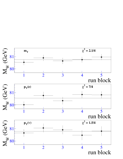
FIG. 55.: The fitted $W$ boson masses in bins of run blocks from the $m_{T}$, $p_{T}(e)$, and $p_{T}(\nu)$ fits. The solid line is the central value for the respective fit over the entire sample. The $W$ fit statistical error for each subsample is shown. The average instantaneous luminosity in the bins is 4.2, 6.1, 7.1, 9.3 and 10.1 respectively, in units of $10^{30}$/cm²/s.

C Dependence on $u_{T}$ Cut

We change the cuts on the recoil momentum $u_{T}$ and study how well the fast Monte Carlo simulation reproduces the variations in the spectra. We split the $W$ sample into subsamples with $u_{\parallel}>0~{}\mbox{GeV}$ and $u_{\parallel}<0~{}\mbox{GeV}$, and fit the subsamples with corresponding Monte Carlo spectra generated with the same cuts. The difference in the fitted masses from the two subsamples corresponds to 0.3$\sigma$, 0.8$\sigma$ and 1.3$\sigma$ for the $m_{T}$, $p_{T}(e)$, and $p_{T}(\nu)$ fits respectively, based on the statistical uncertainty alone. Although there is significant variation among the shapes of the spectra for the different cuts, the fast Monte Carlo models them well.

D Dependence on Fiducial Cuts

We fit the $m_{T}$ spectrum from the $W$ sample and the $m(ee)$ spectrum from the $Z$ sample for different pseudorapidity cuts on the electron direction. Keeping the upper $\mid\!\!\eta_{\rm det}(e)\!\!\mid$ cut fixed at 2.5, we vary the lower $\mid\!\!\eta_{\rm det}(e)\!\!\mid$ cut from 1.5 to 1.7. Similarly, we vary the upper $\mid\!\!\eta_{\rm det}(e)\!\!\mid$ cut from 2.0 to 2.5, keeping the lower $\mid\!\!\eta_{\rm det}(e)\!\!\mid$ cut fixed at 1.5. Figures 56–58 show the change in the $W$ mass versus the $\eta_{\rm det}(e)$ cut using the electron energy scale calibration from the corresponding $Z$ sample. The shaded region indicates the statistical error. Within the uncertainties, the mass is independent of the $\eta_{\rm det}(e)$ cut.

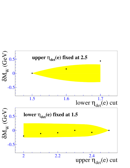
FIG. 56.: The variation in the $W$ mass from the $p_{T}(e)$ fit versus the $\eta_{\rm det}(e)$ cut. The shaded region is the expected statistical variation.

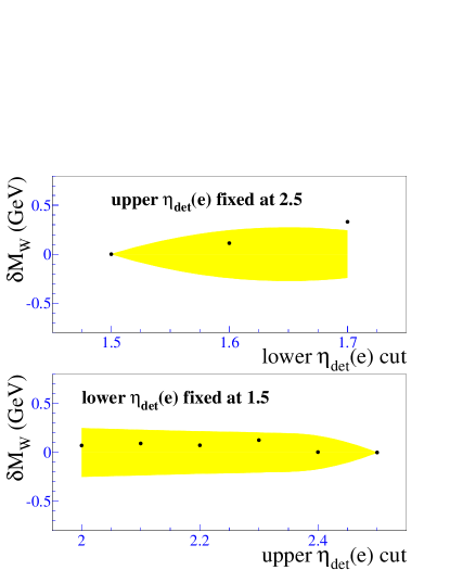
FIG. 57.: The variation in the $W$ mass from the $m_{T}$ fit versus the $\eta_{\rm det}(e)$ cut. The shaded region is the expected statistical variation.

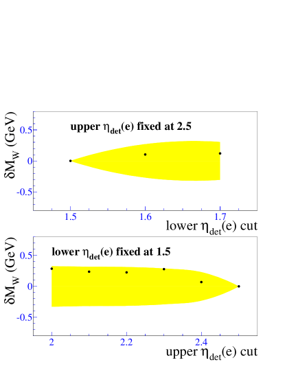
FIG. 58.: The variation in the $W$ mass from the $p_{T}(\nu)$ fit versus the $\eta_{\rm det}(e)$ cut. The shaded region is the expected statistical variation.

E $Z$ Boson Transverse Mass Fits

As a consistency check, we fit the transverse mass distribution of the $Z\rightarrow ee$ events, reconstructed using each electron and the recoil. The measured energy of the second electron is ignored, both in the data and in the Monte Carlo used to obtain the templates. Each $Z$ event is treated (twice) as a $W$ event, where the neutrino transverse momentum is recomputed using the first electron and the recoil. One of the two electrons is required to be in the EC. The fitting range is $70<m_{T}<90$ GeV for the CC/EC events and $70<m_{T}<100$ GeV for the EC/EC events. Figure 59 shows the results. The CC/EC fit yields $M_{Z}=92.004\pm 0.895$(stat) GeV with $\chi^{2}$/dof = 7/9. The EC/EC fit yields $M_{Z}=91.074\pm 0.299$(stat) GeV with $\chi^{2}$/dof = 16/14. The average fitted mass is $M_{Z}=91.167\pm 0.284$(stat) GeV. The fits are good and the fitted masses are consistent with the input $Z$ mass.

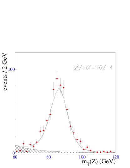
FIG. 59.: Spectra of the $Z$ boson transverse mass, from the CC/EC data (top) and the EC/EC data (bottom). The second electron in the $Z$ boson decay is treated like the neutrino in $W$ boson decay. The superimposed curves show the maximum likelihood fits and the shaded regions show the estimated backgrounds. The $\chi^{2}$/dof between the data and the Monte Carlo are also shown.

XII Uncertainties in the Measurement

Apart from the statistical error in the fitted $W$ mass, uncertainties in the various inputs needed for the measurement lead to uncertainties in the final result. Some of these inputs are discrete (such as the choice of the parton distribution function set) and others are parameterized by continuous variables. For a different choice of pdf set, or a shift in the value of an input parameter by one standard deviation, the expected shift in the fitted $W$ mass is computed by using the fast Monte Carlo to generate spectra with the changed parameter and fitting the spectra with the default templates. The expected shifts due to various input parameter uncertainties (given in Table VI) or choice of pdf set are discussed in detail below, and are summarized in Tables VII and VIII. The shifts in the fitted mass obtained from the different kinematic spectra may be in opposite directions, in which case they are indicated with opposite signs.

TABLE VI.: Errors on the parameters in the $W$ mass analysis. The correlation coefficient between $\alpha_{\rm rec}$ and $\beta_{\rm rec}$ is $-0.98$; that between $s_{\rm rec}$ and $\alpha_{\rm mb}$ is $-0.60$.

parameter	error
parton luminosity $\beta$	0.001 GeV -1
photon coalescing radius $R_{0}$	7 cm
$W$ width	59 MeV
ECEM offset $\delta_{\rm EC}$	0.7 GeV
ECEM scale $\alpha_{\rm EC}$	0.00187
FDC radial scale $\beta_{\rm FDC}$	0.00054
FDC-EC radial scale $\beta_{\rm EC}$	0.0003
ECEM constant term $c_{\rm EC}$	${}^{+0.006}_{-0.01}$
recoil response ($\alpha_{\rm rec}$, $\beta_{\rm rec}$)	(0.06, 0.02)
recoil resolution ($s_{\rm rec}$, $\alpha_{\rm mb}$)	(0.14 GeV1/2, 0.028)
	$\oplus$ (0.0,0.01)
$u_{\parallel}$ correction $\Delta u_{\parallel}$/$\delta\eta\delta\phi$	28 MeV
$u_{\parallel}$ efficiency slope $s$	0.0012 GeV-1

TABLE VII.: Variation in the fitted $M_{W}$ and $M_{Z}$ (in MeV) for the forward electron sample due to variation in the model input parameters by the respective uncertainties.

Source	$\delta M_{Z}$	$\delta M_{Z}$	$\delta M_{W}$	$\delta M_{W}$	$\delta M_{W}$
	(CC/EC)	(EC/EC)	$(m_{T})$	$(p_{T}^{e})$	$(p_{T}^{\nu})$
statistics	124	221	107	128	159
$p_{T}(W)$ spectrum			22	37	44
MRSR2 [47]			$-$11	$-$21	$-$43
MRS(A′) [43]			$-7$	$-43$	$-19$
CTEQ5M [48]			14	9	$-17$
CTEQ4M [49]			1	$-21$	22
CTEQ3M [44]			13	30	28
parton
luminosity $\beta$	8	7	9	11	18
$R_{0}$	10	13	9	17	12
$2\gamma$	5	10	5	10	0
$W$ width			10	10	10
ECEM offset	284	421	437	433	386
ECEM scale
variation 0.0025	114	228	201	201	201
CCEM scale
variation 0.0008	37	0	0	0	0
FDC radial scale	8	36	43	37	28
FDC-EC radial scale	10	52	57	54	48
ECEM constant
term $c_{\rm EC}$	0	0	45	29	78
hadronic
response			11	20	$-50$
hadronic
resolution			40	4	203
$u_{\parallel}$ correction	20	30	18	34	$-6$
$u_{\parallel}$ efficiency			4	$-22$	40
background
normalization	0	11	12	15	25
background
shape	0	5	16	23	78

TABLE VIII.: Variation in the fitted $M_{W}$ and $M_{Z}$ (in MeV) for the central electron sample due to variation in the model input parameters by the respective uncertainties.

Source	$\delta M_{Z}$	$\delta M_{Z}$	$\delta M_{W}$	$\delta M_{W}$	$\delta M_{W}$
	(CC/CC)	(CC/EC)	$(m_{T})$	$(p_{T}^{e})$	$(p_{T}^{\nu})$
statistics	75	124	70	85	105
$p_{T}(W)$ spectrum			10	50	25
MRSR2 [47]			5	26	3
MRS(A′) [43]			$-5$	16	$-31$
CTEQ5M [48]			$-8$	6	$-22$
CTEQ4M [49]			10	11	$-18$
CTEQ3M [44]			0	64	$-9$
parton
luminosity $\beta$	4	8	9	11	9
$R_{0}$	19	10	3	6	0
$2\gamma$	10	5	3	6	0
$W$ width			10	10	10
CC EM offset	387	467	367	359	374
CDC scale	29	33	38	40	52
uniformity			10	10	10
CCEM constant
term $c_{\rm CC}$			23	14	27
hadronic
response			20	16	$-46$
hadronic
resolution			25	10	90
$u_{\parallel}$ correction			15	15	20
$u_{\parallel}$ efficiency			2	$-9$	20
backgrounds			10	20	20

Since the most important parameter, the EM energy scale, is measured by calibrating to the $Z$ mass, we are measuring the ratio of the $W$ and $Z$ boson masses. There can be significant cancellation in uncertainties between the $W$ and $Z$ masses if their variation due to an input parameter change is very similar. For those parameters that affect the fitted $Z$ mass, Tables VII and VIII also show the expected shift in the fitted $Z$ mass. The signed $W$ and $Z$ mass shifts are used to construct a covariance matrix between the various fitted $W$ mass results, which is used to obtain the final $W$ mass value and uncertainty; thus simple combination of the uncertainties in Tables VII and VIII is inappropriate. This is discussed in detail in Section XIII.

A Statistical Uncertainties

Tables VII and VIII list the uncertainties in the $W$ mass measurement due to the finite sizes of the $W$ and $Z$ samples used in the fits to the $m_{T}$, $p_{T}(e)$, $p_{T}(\nu)$, and $m(ee)$ spectra. The statistical uncertainty due to the finite $Z$ sample propagates into the $W$ mass measurement through the electron energy scale $\alpha_{\rm EC}$.

Since the $m_{T}$, $p_{T}(e)$ and $p_{T}(\nu)$ fits are performed using the same $W$ data set, the results from the three fits are statistically correlated. The correlation coefficients between the respective statistical errors are calculated using Monte Carlo ensembles, and are shown in Table IX.

TABLE IX.: The statistical correlation coefficients obtained from Monte Carlo ensemble tests fitting the $W$ boson mass for 260 samples of 11,089 events each.

	correlation matrix
	$m_{T}$	$p_{T}(e)$	$p_{T}(\nu)$
$m_{T}$	1	0.634	0.601
$p_{T}(e)$	0.634	1	0.149
$p_{T}(\nu)$	0.601	0.149	1

B $W$ Boson Production and Decay Model

1 Sources of Uncertainty

Uncertainties in the $W$ boson production and decay model arise from the following sources: the phenomenological parameters in the calculation of the $p_{T}(W)$ spectrum, the choice of parton distribution functions, radiative decays, and the $W$ boson width. In the following we describe how we assess the size of the systematic uncertainties introduced by each of these. We summarize the size of the uncertainties in Tables VII and VIII.

2 $W$ Boson $p_{T}$ Spectrum

In Sec. VIII of Ref. [4], we described our constraint on the $W$ boson $p_{T}$ spectrum. This constraint was obtained by studying the $Z$ boson $p_{T}$ spectrum, which can be measured well using the two electrons in $Z\to ee$ decays. For any chosen parton distribution function, the parameters of the theoretical model were tuned so that the predicted $Z$ boson $p_{T}$ spectrum after simulating all detector effects agreed with the data. The precision with which the parameters could be tuned was limited by the statistical uncertainty and the uncertainty in the background. These parameter values were used to predict the $W$ boson $p_{T}$ spectrum.

The uncertainties in the fitted $W$ boson mass for the CC $W$ sample due to the uncertainty in the $W$ boson $p_{T}$ spectrum were listed in Ref. [4], and are reproduced in Table VIII. The corresponding uncertainty in the EC analysis is given in Table VII. The CC and EC $W$ mass uncertainties from this source are assumed to be fully correlated.

3 Parton Distribution Functions

To quantify the $W$ mass uncertainty due to variations in the input parton distribution functions, we select the MRS(A^′), MRSR2, CTEQ5M, CTEQ4M and CTEQ3M sets to compare to MRST. We select these sets because their predictions for the lepton charge asymmetry in $W$ decays and the neutron-to-proton Drell-Yan ratio span the range of consistency with the measurements from CDF [51] and E866 [52]. These measurements constrain the ratio of $u$ and $d$ quark distributions which have the most influence on the $W$ rapidity spectrum.

Using these parton distribution function sets as input to the fast Monte Carlo model, we generate $m_{T}$ and lepton $p_{T}$ spectra. For each chosen parton distribution function set we use the appropriate $W$ boson $p_{T}$ spectrum as used in our CC $W$ mass analysis. We then fit the generated spectra in the same way as the spectra from collider data, i.e. using MRST parton distribution functions. Table VII lists the variation of the fitted EC $W$ mass values relative to MRST. The CC and EC $W$ mass uncertainty from this source is taken to be fully correlated, taking the relative signs of the mass shifts into account.

We find that the combination of the CC and EC $W$ boson mass measurements is less sensitive to pdf variations, than for the CC measurement alone. The pdf uncertainty on the CC measurement is 11 MeV. The pdf uncertainty on the CC+EC combined measurement is 7 MeV. As expected, the larger combined rapidity coverage makes the observed transverse mass and transverse momentum distributions less sensitive to the longitudinal boost of the $W$ boson.

4 Parton Luminosity

The uncertainty of $10^{-3}\ \mbox{GeV}^{-1}$ in the parton luminosity slope $\beta$ (Sec. V) translates into an uncertainty in the fitted $W$ and $Z$ boson masses. We estimate the sensitivity in the fitted $W$ and $Z$ masses by fitting Monte Carlo spectra generated with different values of $\beta$. The uncertainty in $\beta$ is taken to be fully correlated between the CC and EC $W$ mass analyses.

5 Radiative Decays

We assign an error to the modeling of radiative decays based on varying the detector parameter $R_{0}$ (Sec. V). $R_{0}$ defines the maximum separation between the photon and electron directions above which the photon energy is not included in the electron shower. In general, radiation shifts the fitted mass down for the transverse mass and electron fits, because for a fraction of the events the photon energy is subtracted from the electron. Hence increasing $R_{0}$ decreases the radiative shift. Both the fitted $W$ and $Z$ masses depend on $R_{0}$. To estimate the systematic error, we fit Monte Carlo spectra generated with different values of $R_{0}$. geant detector simulations show that, for an $R_{0}$ variation of $\pm 7$ cm, the electron-photon cluster overlap changes to give the maximum variation in the electron identification efficiency. The changes in the mass fits when varying $R_{0}$ by $\pm 7$ cm are listed in Table VII.

There are also theoretical uncertainties in the radiative decay calculation. Initial state QED radiation is not included in the calculation of Ref. [40]. However, initial state radiation does not affect the kinematic distributions used to fit the mass in the final state. We studied the effect of QED radiation off the initial state quarks on the parton luminosity by computing the parton luminosity including and excluding QED radiative effects on the quark momentum distribution. The change in the parton luminosity slope parameter was less then half of the quoted uncertainty on the parameter, which was dominated by acceptance effects.

The calculation of Ref. [40] includes only processes in which a single photon is radiated. We use the code provided by the authors of Ref. [53] to estimate the shift introduced in the measured $W$ and $Z$ masses by neglecting two-photon emission. The estimated shifts in the $W$ and $Z$ fitted masses due to two-photon radiation are shown in Table VII. Since this effect is an order of magnitude smaller than the statistical uncertainty in our measurement we do not correct for it, but add it in quadrature to the uncertainty due to radiative corrections. The uncertainty in the radiative correction is taken to be fully correlated between the CC and EC $W$ mass analyses.

6 $W$ Boson Width

The uncertainty on the fitted $W$ mass corresponds to the uncertainty in the measured value of the $W$ boson width $\Gamma_{W}$ = 2.062$\pm$0.059 GeV [35]. We take this uncertainty to be fully correlated between the CC and EC $W$ mass analyses.

Our recent measurement of the $W$ width [54] considerably improves the precision of $\Gamma_{W}$ and would reduce the $W$ mass uncertainty from this source. However, since this is already a small source of uncertainty, the impact on the total $W$ mass uncertainty is small.

C Detector Model Parameters

The uncertainties on the parameters of the detector model determined in Secs. VI–VII translate into uncertainties in the $W$ mass measurement. We study the sensitivity of the $W$ mass measurement to the values of the parameters by fitting the data with spectra generated by the fast Monte Carlo with input parameters modified by $\pm$1 standard deviation.

Table VII lists the variation in the measured EC $W$ mass due to variation in the individual parameters. For each item the uncertainty is determined with a typical Monte Carlo statistical error of 5 MeV. To achieve this precision, 10–20 million $W\to e\nu$ decays are simulated for each item.

The residual calorimeter nonlinearity is parametrized by the offset $\delta_{\rm EC}$. The electron momentum resolution is parametrized by $c_{\rm EM}$. The electron angle calibration includes the effects of the parameters $\beta_{\rm FDC}$ and $\beta_{\rm EC}$, discussed in Section VI. The recoil response is parameterized by $\alpha_{\rm rec}$ and $\beta_{\rm rec}$. The recoil resolution is parameterized by $s_{\rm rec}$ and $\alpha_{\rm mb}$. Electron removal refers to the bias $\Delta u_{\parallel}$ introduced in the $u_{\parallel}$ measurement by the removal of the cells occupied by the electron. Selection bias refers to the $u_{\parallel}$ efficiency.

D Backgrounds

We determine the sensitivity of the fit results to the assumed background normalizations and shapes by repeating the fits to the data with background shapes and normalizations modified by $\pm$1 standard deviation. Table VII lists the uncertainties introduced in the EC $W$ boson mass measurement.

XIII Combined EC and CC $W$ Boson Mass Error Analysis

The measurement of the $W$ mass requires the knowledge of many parameters in our model of the $W$ production, decay and detector response. These parameters are constrained by measurements, and in some cases by theoretical input. The $W$ mass error analysis involves the propagation of the measurement or theoretical uncertainties to the error matrix on the parameters, which is then propagated further to the error matrix on the CC and EC $W$ mass measurements. The error matrix allows us to combine the fitted $W$ mass values using the different data samples and techniques into a single value with a combined error.

We identify the following parameters of relevance to the $W$ mass measurements in the EC and CC:

• $W$ mass statistical errors $\delta\omega_{\rm CC}$ and $\delta\omega_{\rm EC}$

• EM scales $\alpha_{\rm CC}$ and $\alpha_{\rm EC}$

• EM offset parameters $\delta_{\rm CC}$ and $\delta_{\rm EC}$

• FDC scale $\beta_{\rm FDC}$ and FDC-EC relative scale $\beta_{\rm EC}$

• CDC scale $\beta_{\rm CDC}$

• EM resolutions (constant terms) $c_{\rm CC}$ and $c_{\rm EC}$

• recoil response $\vec{a}_{\rm rec}$ representing jointly the response parameters $\alpha_{\rm rec}$ and $\beta_{\rm rec}$

• recoil resolution $\vec{q}_{\rm rec}$ representing jointly the hadronic sampling term $s_{\rm rec}$ and the effects of the underlying event $\alpha_{\rm mb}$

• backgrounds $b_{\rm CC}$ and $b_{\rm EC}$

• $u_{||}$ corrections $u_{\rm CC}$ and $u_{\rm EC}$

• $u_{||}$ efficiencies $\varepsilon_{\rm CC}$ and $\varepsilon_{\rm EC}$

• radiative corrections as a function of the photon coalescing radius $R_{0}$

• parton luminosity $\beta$

• theoretical modeling $\vec{t}$

We take the EM scales, EM offsets, angular scales, $u_{||}$ corrections, parton luminosity and the radiative correction to be a set of parameters that jointly determine the measured $W$ and $Z$ masses. We also take the EM resolution parameters as a correlated set. We take the CC and EC backgrounds and $u_{||}$ efficiencies to be uncorrelated. The recoil modelling and the theoretical modelling (including pdf’s, $p_{T}(W)$ spectrum, parton luminosity, radiative corrections and $W$ width) are treated as being common between the CC and the EC analyses. For all correlated parameters the sign of the $W$ mass correlation is determined by the relative sign of the mass shifts.

The following measurements provide information on the values of these parameters

• The $Z$ mass measurements $M_{Z}^{\rm CC/CC}$, $M_{Z}^{\rm CC/EC}$ and $M_{Z}^{\rm EC/EC}$

• FDC radial calibration $\theta_{\rm FDC}$ and FDC-EC relative radial calibration $\theta_{\rm EC}$

• CDC $z$ calibration $\theta_{\rm CDC}$

• CC and EC EM offset measurements $o_{\rm CC}$ and $o_{\rm EC}$

• Gaussian width fitted to $Z$ boson peak $\sigma_{Z}^{\rm CC/CC}$, $\sigma_{Z}^{\rm CC/EC}$ and $\sigma_{Z}^{\rm EC/EC}$

• $p_{T}$ balance in $Z$ events

• width of $p_{T}$ balance in $Z$ events

• measurements of $u_{\parallel}$ correction and $u_{\parallel}$ efficiency

• constraints on theoretical model (boson $p_{T}$ from DØ data, $W$ width from world data including DØ data, and pdf’s and parton luminosity from world data)

We express the variations on the various calibration quantities (such as $Z$ mass, EM offset, and angular scales, collectively referred to as $\vec{C}$) and the $Z$ width measurements as a linear combination of the variations on the parameters

$$\delta\vec{C} = \Delta_{C}\;\delta\vec{p}$$ (55)

$$\delta\vec{\sigma}_{Z} = \Delta_{\sigma}\;\delta\vec{c}_{\rm EM}$$ (56)

where

$$\delta\vec{C} = (\delta M_{Z}^{\rm CC/CC},\delta M_{Z}^{\rm CC/EC},\delta M_{Z}^{\rm EC/EC},\delta\theta_{\rm FDC},\delta\theta_{\rm EC},$$ (58)

$$\delta\theta_{\rm CDC},\delta o_{\rm CC},\delta o_{\rm EC},\delta R_{0},\delta u_{\rm CC},\delta u_{\rm EC},\delta\beta),$$

$$\delta\vec{p} = (\delta\alpha_{\rm CC},\delta\alpha_{\rm EC},\delta\beta_{\rm FDC},\delta\beta_{\rm EC},\delta\beta_{\rm CDC},$$ (60)

$$\delta\delta_{\rm CC},\delta\delta_{\rm EC},\delta R_{0},\delta u_{\rm CC},\delta u_{\rm EC},\delta\beta)$$

and

$$\delta\vec{\sigma}_{Z} = (\delta\sigma_{Z}^{\rm CC/CC},\delta\sigma_{Z}^{\rm CC/EC},\delta\sigma_{Z}^{\rm EC/EC}),$$ (61)

$$\delta\vec{c}_{\rm EM} = (\delta c_{\rm CC},\delta c_{\rm EC}).$$ (62)

The $\Delta$ matrices contain the partial derivatives of the observables with respect to the parameters.

Similarly, the variations on the $W$ mass are related linearly to the parameter variations

$$\delta\vec{M}_{W} = \Delta_{W}\;\delta\vec{p}$$ (63)

$$+ \Delta_{\sigma_{W}}\;\delta\vec{c}_{\rm EM}$$ (64)

$$+ \Delta_{\rm recoil\;scale}\;\delta\vec{a}_{\rm rec}$$ (65)

$$+ \Delta_{\rm recoil\;resolution}\;\delta\vec{q}_{\rm rec}$$ (66)

$$+ \Delta_{\rm background}\;\delta\vec{b}$$ (67)

$$+ \Delta_{\rm u}\;\delta\vec{u}$$ (68)

$$+ \Delta_{\varepsilon}\;\delta\vec{\varepsilon}$$ (69)

$$+ \Delta_{\rm theory}\;\delta\vec{t}$$ (70)

$$+ \delta\vec{\omega}$$ (71)

where $\delta\vec{M}_{W}=(\delta M_{W}^{\rm CC},\delta M_{W}^{\rm EC})$.

Knowing the components of $\delta\vec{C}$ and $\delta\vec{\sigma}_{Z}$, we compute the covariance matrix for the parameters in $\vec{p}$ and $\vec{c}_{\rm EM}$. Since there are more measurements than parameters, we use the generalized least squares fitting procedure for this purpose. We then propagate the parameter covariance matrices into the covariance matrix for the CC and EC $W$ mass measurements using equation 71, by identifying the covariance matrix with the expected value of $\delta\vec{M}_{W}(\delta\vec{M}_{W})^{T}$, where $T$ indicates the transpose. The various contributions to $\delta\vec{M}_{W}$ are independent, hence they contribute additively to the total covariance matrix.

The CC $W$ mass measurements [4] were obtained using the MRS(A^′) parton distribution functions. We adjust these measurements by the estimated shifts (see Table VIII) when using the MRST parton distribution functions. Thus we use the following $W$ mass values extracted from the CC data to combine with our EC measurements:

$$M_{W}^{\rm CC} = 80.443\;{\rm GeV}\;(m_{T}\ {\rm fit})$$ (72)

$$M_{W}^{\rm CC} = 80.459\;{\rm GeV}\;(p_{T}(e)\ {\rm fit})$$ (73)

$$M_{W}^{\rm CC} = 80.401\;{\rm GeV}\;(p_{T}(\nu)\ {\rm fit})$$ (74)

The combined $W$ mass $M_{W}$ for a set of $n$ $W$ mass measurements $m_{i}$ and their covariance matrix $V$ is given by

$$M_{W}=(\sum_{i,j=1}^{n}{H_{ij}}\,\,m_{j})\,/\,(\,\sum_{i,j=1}^{n}{H_{ij}}\,),$$ (75)

where $H\equiv V^{-1}$ and $i,j$ run over the $W$ mass measurements being combined. The combined error is given by

$$\sigma(M_{W})=(\,\sum_{i,j=1}^{n}{H_{ij}}\,)^{-1/2},$$ (76)

and the $\chi^{2}$ for the combination is given by

$$\chi^{2}=\sum_{i,j=1}^{n}{(m_{i}-M_{W})\,\,H_{ij}\,\,(m_{j}-M_{W})}.$$ (77)

XIV Results

We use the covariance matrix described above to obtain the total uncertainty on the EC $W$ mass measurements and to combine our CC and EC measurements. We obtain the following results for the transverse mass fit

$$M_{W}^{\rm EC} = 80.757\pm 0.107({\rm stat})\pm 0.204({\rm syst})\ \hbox{GeV}$$ (78)

$$= 80.757\;\pm\;0.230\;{\rm GeV}$$ (79)

and

$$M_{W} = 80.504\;\pm\;0.097\;{\rm GeV}\;({\rm CC\;{\rm and}\;EC\;combined}).$$ (80)

The $\chi^{2}$ for the CC+EC $m_{T}$ combination is 1.5 for one degree of freedom, with a probability of 23%.

Similarly, for the $p_{T}(e)$ fit we obtain

$$M_{W}^{\rm EC} = 80.547\pm 0.128({\rm stat})\pm 0.203({\rm syst})\ \hbox{GeV}$$ (81)

$$= 80.547\;\pm\;0.240\;{\rm GeV}$$ (82)

and

$$M_{W} = 80.480\;\pm\;0.126\;{\rm GeV}\;({\rm CC\;{\rm and}\;EC\;combined}).$$ (83)

The $\chi^{2}$ for the CC+EC $p_{T}(e)$ combination is 0.1 with a probability of 74%.

For the $p_{T}(\nu)$ fit we obtain

$$M_{W}^{\rm EC} = 80.740\pm 0.159({\rm stat})\pm 0.310({\rm syst})\ \hbox{GeV}$$ (84)

$$= 80.740\;\pm\;0.348\;{\rm GeV}$$ (85)

and

$$M_{W} = 80.436\;\pm\;0.171\;{\rm GeV}\;({\rm CC\;{\rm and}\;EC\;combined}).$$ (86)

The $\chi^{2}$ for the CC+EC $p_{T}(\nu)$ combination is 1.0 with a probability of 32%.

The combination of the $m_{T}$, $p_{T}(e)$ and $p_{T}(\nu)$ fit values for the EC give the combined EC $W$ mass result

$$M_{W}=80.691\;\pm\;0.227\;{\rm GeV}.$$ (87)

The $\chi^{2}$/dof is 4.0/2, with a probability of 14%.

We combine all six measurements (CC and EC fits with the three techniques) to obtain the combined 1994–1995 measurement

$$M_{W} = 80.498\;\pm\;0.095\;{\rm GeV}.$$ (88)

The $\chi^{2}$/dof is 5.1/5, with a probability of 41%. The consistency of the six results indicates that we understand the ingredients of our model and their uncertainties. Including the measurement from the 1992–1993 data gives the 1992–1995 data measurement:

$$M_{W} = 80.482\;\pm\;0.091\;{\rm GeV}.$$ (89)

Table X lists the DØ $W$ mass measurement uncertainties from the 1994–1995 end calorimeter data alone and the combined 1994–1995 central and end calorimeter data.

TABLE X.: $W$ mass uncertainties (in MeV) in the EC measurement and the combined CC+EC measurement from the 1994–1995 data.

Source	EC	CC+EC
$W$ statistics	108	61
$Z$ statistics	181	59
calorimeter linearity	52	25
calorimeter uniformity	–	8
electron resolution	42	19
electron angle calibration	20	10
recoil response	17	25
recoil resolution	42	25
electron removal	4	12
selection bias	5	3
backgrounds	20	9
pdf	17	7
parton luminosity	2	4
$p_{T}(W)$	25	15
$\Gamma(W)$	10	10
radiative corrections	1	12

The DØ measurement is in good agreement with other measurements and is more precise than previously published results. Table XI lists previously published measurements with uncertainties below 500 MeV, except previous DØ measurements which are subsumed into this measurement. A global fit to all electroweak measurements excluding the direct $W$ mass measurements predicts $M_{W}=80.367\pm 0.029$ GeV [11]. Figure 60 gives a graphical representation of these data.

TABLE XI.: Previously published measurements of the $W$ boson mass.

measurement	$M_{W}$ (GeV)	reference
CDF 90	79.910$\pm$0.390	[55]
UA2 92	80.360$\pm$0.370	[12]
CDF 95	80.410$\pm$0.180	[13]
L3 99	80.610$\pm$0.150	[14]
ALEPH 99	80.423$\pm$0.124	[15]
OPAL 99	80.380$\pm$0.130	[16]
DELPHI 99	80.270$\pm$0.145	[17]
DØ 99 combined (this result)	80.482$\pm$0.091

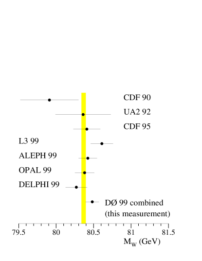
FIG. 60.: A comparison of this measurement with previously published $W$ boson mass measurements (Table XI). The shaded region indicates the predicted $W$ boson mass value from global fits to all electroweak data except the $W$ mass measurements [11].

We evaluate the radiative corrections $\Delta r_{EW}$, defined in Eq. 1. Our measurement of $M_{W}$ from Eq. 89 leads to

$$\Delta r_{EW}=-0.0322\pm 0.0059,$$ (90)

5.5 standard deviations from the tree level value, demonstrating the need for higher-order electroweak loop corrections. In Fig. 61 we compare the measured $W$ boson and top quark masses [20] from DØ with the values predicted by the standard model for a range of Higgs mass values [56]. Also shown is the prediction from the calculation in Ref. [22] for a model involving supersymmetric particles assuming the chargino, Higgs, and left-handed selectron masses are greater than 90 GeV. The measured values are in agreement with the prediction of the standard model, and in even better agreement with a supersymmetric extension of the standard model.

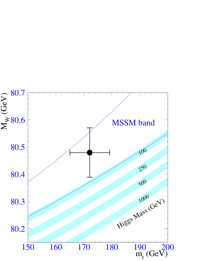
FIG. 61.: A comparison of the $W$ boson and top quark mass measurements by the DØ collaboration with the standard model predictions for different Higgs boson masses [56]. The width of the bands for each Higgs boson mass value indicates the uncertainty due to the error in $\alpha(M_{Z}^{2})$. Also shown is the range allowed by the MSSM [22].

REFERENCES

- [1] B. Abbott et al. (DØ Collaboration), FERMILAB-Pub-99/259-E, hep-ex/9909030, to be published in Phys. Rev. Lett.
- [2] S. Abachi et al. (DØ Collaboration), Nucl. Instrum. Methods in Phys. Res. A 338, 185 (1994).
- [3] H. Aihara et al., Nucl. Instrum. Methods in Phys. Res. A 325, 393 (1993).
- [4] B. Abbott et al. (DØ Collaboration), Phys. Rev. D 58, 092003 (1998); B. Abbott et al. (DØ Collaboration), Phys. Rev. Lett. 80, 3008 (1998).
- [5] S. Abachi et al. (DØ Collaboration), Phys. Rev. Lett. 77, 3309 (1996); B. Abbott et al. (DØ Collaboration), Phys. Rev. D 58, 012002 (1998).
- [6] G. Arnison et al. (UA1 Collaboration), Phys. Lett. B 122, 103 (1983).
- [7] M. Banner et al. (UA2 Collaboration), Phys. Lett. B 122, 476 (1983).
- [8] G. Arnison et al. (UA1 Collaboration), Phys. Lett. B 126, 398 (1983);
- [9] P. Bagnaia et al. (UA2 Collaboration), Phys. Lett. B 129, 130 (1983).
- [10] S.L. Glashow, Nucl. Phys. 22, 579 (1961); S. Weinberg, Phys. Rev. Lett. 19, 1264 (1967); A. Salam, in Proceedings of the 8th Nobel Symposium, ed. N. Svartholm (Almqvist and Wiksells, Stockholm, 1968), p. 367.
- [11] The LEP collaborations, the LEP Electroweak Working Group, and the SLD Heavy Flavour and Electroweak Groups, CERN-EP/99-15 (unpublished) and references therein.
- [12] J. Alitti et al. (UA2 Collaboration), Phys. Lett. B 276, 354 (1992). The value quoted in Table XI uses from Eq. 2.
- [13] F. Abe et al. (CDF Collaboration), Phys. Rev. Lett. 75, 11 (1995) and Phys. Rev. D 52, 4784 (1995).
- [14] M. Acciarri et al. (L3 Collaboration), Phys. Lett. B 454, 386 (1999).
- [15] R. Barate et al. (ALEPH Collaboration), Phys. Lett. B 453 121 (1999).
- [16] K. Ackerstaff et al. (OPAL Collaboration), Phys. Lett. B 453 138 (1999).
- [17] P. Abreu et al. (DELPHI Collaboration), CERN-EP-99-079, submitted to Phys. Lett. B.
- [18] A. Sirlin, Phys. Rev. D 22, 971 (1980); W. Marciano and A. Sirlin, Phys. Rev. D 22, 2695 (1980) and erratum-ibid. 31, 213 (1985).
- [19] C. Caso et al., Review of Particle Physics, Eur. Phys. J. C3 (1998).
- [20] DØ Collaboration, B. Abbott et al., Phys. Rev. Lett. 80, 2063 (1998); DØ Collaboration, B. Abbott et al., Phys. Rev. D 60, 052001 (1999) and references therein.
- [21] F. Abe et al. (CDF Collaboration), Phys. Rev. Lett. 82, 271 (1999), erratum-ibid. 82, 2808 (1999) and references therein.
- [22] P. Chankowski et al., Nucl. Phys. B417, 101 (1994); D. Garcia and J. Sola, Mod. Phys. Lett. A 9, 211 (1994); A. Dabelstein, W. Hollik and W. Mosle, in Perspectives for Electroweak Interactions in Collisions, ed. by B. A. Kniehl (World Scientific, Singapore, 1995) p. 345; D. Pierce et al., Nucl. Phys. B491, 3 (1997).
- [23] H.T. Edwards, in Annual Review of Nuclear and Particle Science, Vol. 35, ed. J.D. Jackson et al., (Annual Reviews, Palo Alto, 1985) p. 605.
- [24] R.D. Schamberger, in Proceedings of the Fifth International Conference on Calorimetry in High Energy Physics, Upton, New York, 1994, edited by Howard Gordon and Doris Rueger (World Scientific, Singapore, 1994); J. Kotcher, in Proceedings of the 1994 Beijing Calorimetry Symposium, Beijing, China, 1994, p. 144; J. A. Guida, in Proceedings of the 4th International Conference on Advanced Technology and Particle Physics, Como, Italy, 1994, Nucl. Phys. Suppl. Vol. B44, 158 (1995).
- [25] S. Abachi et al., Nucl. Instrum. Methods in Phys. Res. A 324, 53 (1993).
- [26] J.W.T. McKinley, Ph.D. thesis, Michigan State University, 1996 (unpublished).
- [27] R. Brun, F. Bruyant, M. Maire, A.C. McPherson and P. Zanarini, geant 3, CERN DD/EE/84-1 (1987); F. Carminati et al., geant Users Guide, CERN Program Library W5013, 1991 (unpublished).
- [28] S. Abachi et al. (DØ Collaboration), Phys. Rev. D 52, 4877 (1995).
- [29] G.A. Ladinsky and C.P. Yuan, Phys. Rev. D 50, 4239 (1994).
- [30] P.B. Arnold and R.P. Kauffman, Nucl. Phys. B349, 381 (1991).
- [31] P.B. Arnold and M.H. Reno, Nucl. Phys. B319, 37 (1989) and erratum-ibid. B330, 284 (1990).
- [32] J. Collins and D. Soper, Nucl. Phys. B193, 381 (1981) and erratum-ibid. B213, 545 (1983); J. Collins, D. Soper, and G. Sterman, Nucl. Phys. B250, 199 (1985).
- [33] G. Altarelli, R.K. Ellis, M. Greco and G. Martinelli, Nucl. Phys. B246, 12 (1984).
- [34] A.D. Martin, R.G. Roberts, W.J. Stirling, and R.S. Thorne, Eur. Phys. J. C4, 463 (1998).
- [35] S. Abachi et al. (DØ Collaboration), Phys. Rev. Lett. 75, 1456 (1995).
- [36] G. Marchesini et al., Comput. Phys. Commun. 67 465 (1992), release 5.7.
- [37] H. Plotow-Besch, CERN-PPE W5051 (1997), release 7.02 (unpublished).
- [38] E. Mirkes, Nucl. Phys. B387, 3 (1992).
- [39] J. Collins and D. Soper, Phys. Rev. D 16, 2219 (1977).
- [40] F.A. Berends and R. Kleiss, Z. Phys. C 27, 365 (1985); F.A. Berends, R. Kleiss, J.P. Revol, J.P. Vialle, Z. Phys. C 27, 155 (1985).
- [41] J. Bantly, Ph.D. thesis, Northwestern University, 1992 (unpublished).
- [42] B. Abbott et al. (DØ Collaboration), Nucl. Instrum. Methods in Phys. Res. A 424, 352 (1999).
- [43] A.D. Martin, W.J. Stirling, and R.G. Roberts, Phys. Rev. D 50, 6734 (1994) and Phys. Rev. D 51, 4756 (1995).
- [44] H.L. Lai et al., Phys. Rev. D 51, 4763 (1995).
- [45] J. Botts et al., Phys. Lett. B 304, 159 (1993).
- [46] A.D. Martin, W.J. Stirling, and R.G. Roberts, Phys. Lett. B 306, 145 (1993) and erratum-ibid. B 309, 492 (1993).
- [47] A.D. Martin, R.G. Roberts and W.J. Stirling, Phys. Lett. B 387, 419 (1996).
- [48] H.L. Lai et al., hep-ph/9903282 (unpublished).
- [49] H.L. Lai et al., Phys. Rev. D 55, 1280 (1997).
- [50] B. Abbott et al. (DØ Collaboration), FERMILAB-PUB-99-197-E, hep-ex/9907009, submitted to Phys. Rev. D.
- [51] F. Abe et al. (CDF Collaboration), Phys. Rev. Lett. 81, 5754 (1998).
- [52] E.A. Hawker et al. (Fermilab E866/NuSea Collaboration), Phys. Rev. Lett. 80, 3715 (1998); J.C. Peng et al. (Fermilab E866/NuSea Collaboration), Phys. Rev. D 58, 092004 (1998).
- [53] U. Baur et al., Phys. Rev. D 56, 140 (1997); U. Baur, S. Keller, and W.K. Sakumoto, Phys. Rev. D 57, 199 (1998).
- [54] B. Abbott et al. (DØ Collaboration), FERMILAB-PUB-99-171-E, hep-ex/9906025, submitted to Phys. Rev. D.
- [55] F. Abe et al. (CDF Collaboration), Phys. Rev. Lett. 65, 2243 (1990) and Phys. Rev. D 43, 2070 (1991).
- [56] G. Degrassi et al. Phys. Lett. B 418, 209 (1998); G. Degrassi, P. Gambino, and A. Sirlin, Phys. Lett. B 394, 188 (1997).