Application of Bayesian probability theory to the measurement of binomial data at past and future Tevatron experiments

Abstract

The experimental problem of converting a measured binomial quantity, the fraction of events in a sample that pass a cut, into a physical binomial quantity, the fraction of events originating from a signal source, is described as a system of linear equations. This linear system illustrates several familiar aspects of experimental data analysis. Bayesian probability theory is used to find a solution to this binomial measurement problem that allows for the straightforward construction of confidence intervals. This solution is also shown to provide an unbiased formalism for evaluating the behavior of data sets under different choices of cuts, including a cut designed to increase the significance of a possible, albeit previously unseen, signal.

Several examples are used to illustrate the features of this method, including the discovery of the top quark and searches for new particles produced in association with $W^{\pm}$ bosons. It is also demonstrated how to use this method to make projections for the potential discovery of a Standard Model Higgs boson at a Tevatron Run 2 experiment, as well as the utility of measuring the integrated luminosity through inclusive $p\overline{p}\rightarrow W^{\pm}$ production.

I Introduction

A set of experimental data is almost always presented in terms of the subset of interesting events, called the signal, and a complimentary subset of events from non-interesting sources, called the background. The fraction of events from each subset is a binomial quantity; some fraction of the sample is either characterized as signal or it is not. There is usually no exact means of separating signal events from background events. Instead an experimental cut is imposed on the original sample. Such a cut is motivated by independent studies that imply the cut will be more efficient for the events of interest than for the non-interesting events. After this cut is applied, estimates are made regarding the amount of signal and background in these new binomial subsets: those events that survived the cut, and those that failed the cut.

The attempt to rotate data from the experimental axis in pass-fail space onto the physics axis that defines signal-background space is referred to in this paper as the measurement problem. The measurement problem is introduced and described in Section II. The classical treatment of the measurement problem as a system of linear equations provides some insight into the practical business of analyzing data, but it is found to be inadequate for the construction of confidence intervals. A Bayesian analysis of related binomial quantities provides a straightforward solution to this problem. Bayesian descriptions of binomial data are given in Section III. A full solution to the measurement problem is found in Section IV.

The solution of Section IV provides a result in terms of the fraction of signal events in the entire original sample; Section V reformulates this solution so that the result can be presented as a fraction of signal events in the subset of events that passed the cut. The methods introduced in Sections IV and V are demonstrated in Example 1 with the data used for the discovery of the top quark. Example 2 describes one way to use this method to estimate the necessary size of control samples in order to understand the background to inclusive $p\overline{p}\rightarrow W^{\pm}$ production.

Section VI presents a formalism for calculating the minimum number of events which must survive a cut designed to enhance the significance of a possible signal over expectations. Section VII describes how to use the measurement problem to attribute a level of confidence in the consistency of a possible new discovery with the original understanding of the expected backgrounds. Examples 3 and 4 illustrate the methods of Sections VI and VII using published $p\overline{p}\rightarrow W^{\pm}+b\overline{b}$ results. Example 5 extrapolates this Tevatron Run 1 data to the estimated amount of data available for a similar analysis in Run 2.

II The Measurement Problem: A Linear System for Data Analysis

The measurement problem is equivalent to taking data that is recorded on an experimental axis, i.e. pass-fail space, and rotating the experimental results onto a physics axis, i.e. signal-background space. When a cut is imposed on a data sample of $N_{Total}$ events, the sample is then divided into a subset of events which pass the cut $N_{pass}$, and a subset of events which fail the cut $N_{fail}$,

$$N_{Total}=N_{pass}+N_{fail}\;.$$ (1)

The original sample can also be described as a subset of signal $N_{sig}$ and background $N_{bkg}$ events,

$$N_{Total}=N_{sig}+N_{bkg}\;.$$ (2)

The different axes are related through a measurement matrix ${\bf M}$,

$$\left(\begin{array}[]{c}N_{pass}\\ N_{fail}\end{array}\right)={\bf M}\left(\begin{array}[]{c}N_{sig}\\ N_{bkg}\end{array}\right)\;.$$ (3)

The measurement problem is to invert the matrix ${\bf M}$ such that

$$\left(\begin{array}[]{c}N_{sig}\\ N_{bkg}\end{array}\right)={\bf M}^{-1}\left(\begin{array}[]{c}N_{pass}\\ N_{fail}\end{array}\right),$$ (4)

where the elements of the measurement matrix are the efficiencies of the cut on the signal and the background,

$${\bf M}\equiv\left(\begin{array}[]{cc}\varepsilon&r\\ 1-\varepsilon&1-r\end{array}\right)\;.$$ (5)

The efficiency $\varepsilon$ of the cut on the signal is defined as the number of signal events that will pass the cut, $S_{pass}$, divided by the total number of signal events in the original sample; the number of signal events which will fail the cut $S_{fail}$ is the total number of signal events times the inefficiency ($1-\varepsilon$):

$$S_{pass} = \varepsilon\>N_{sig}\;,$$ (7)

$$S_{fail} = (1-\varepsilon)\>N_{sig}\;.$$ (8)

The efficiency $\varepsilon$ is always evaluated from some independent control sample of $\varepsilon_{Total}$ diagnostic events, where $\varepsilon_{pass}$ ($\varepsilon_{fail}$) diagnostic events pass (fail) the cut;

$$\varepsilon = \varepsilon_{pass}/\varepsilon_{Total}\;,$$ (10)

$$1-\varepsilon = \varepsilon_{fail}/\varepsilon_{Total}\;.$$ (11)

Similarly the efficiency of the cut on the background $r$, referred to as the ‘rfficiency’, is defined as the number of background events that will pass the cut $B_{pass}$ divided by the total number of background events in the original sample, while the number of background events which will fail the cut $B_{fail}$ is the total number of background events times the ‘inrfficiency’ ($1-r$):

$$B_{pass} = r\>N_{bkg}\;,$$ (13)

$$B_{fail} = (1-r)\>N_{bkg}\;.$$ (14)

Just as the efficiency is evaluated from an independent diagnostic sample, the rfficiency comes from another independent sample of $r_{Total}$ events where $r_{pass}$ ($r_{fail}$) diagnostic events pass (fail) the cut;

$$r = r_{pass}/r_{Total}\;,$$ (16)

$$1-r = r_{fail}/r_{Total}\;.$$ (17)

It is common to refer to the rejection factor $R$ of a cut as the ratio of the different efficiencies

$$R\equiv\frac{\varepsilon}{r}\;,$$ (18)

while the enhancement $E$ of a cut on a given sample can be defined as

$$E\equiv\frac{\varepsilon-r}{r}=R-1\;.$$ (19)

The inverse measurement matrix ${\bf M}^{-1}$ ,

$${\bf M}^{-1}=\frac{1}{\varepsilon-r}\left(\begin{array}[]{cc}1-r&\;-r\\ \varepsilon-1&\;\varepsilon\end{array}\right)\;,$$ (20)

exists only if the determinant of matrix ${\bf M}$ is not equal to zero, which is true whenever $\varepsilon\neq r$. This requirement is naturally satisfied whenever the rejection factor is not equal to one or the enhancement is non-zero. Usually a cut is chosen such that

$$0<r<\varepsilon<1\;.$$ (21)

There is nothing in this formalism which prevents the choice of a cut such that $\varepsilon<r$; this is the situation where the background is enhanced at the expense of the signal.

Once the inverse measurement matrix is known, it is possible to describe the number of signal (or background) events in terms of the number of events which pass (or fail) the cut:

$$N_{sig} = \frac{(1-r)\>N_{pass}-r\>N_{fail}}{\varepsilon-r}$$ (23)

$$= \frac{N_{pass}-r\>N_{Total}}{\varepsilon-r}\;,$$ (24)

$$N_{bkg} = \frac{(\varepsilon-1)\>N_{pass}+\varepsilon\>N_{fail}}{\varepsilon-r}$$ (25)

$$= \frac{\varepsilon\>N_{Total}-N_{pass}}{\varepsilon-r}$$ (26)

$$= \frac{N_{fail}-(1-\varepsilon)\>N_{Total}}{\varepsilon-r}\;.$$ (27)

In fractional terms, defining

$$f_{sig} \equiv N_{sig}/N_{Total}\;,$$ (29)

$$f_{bkg} \equiv N_{bkg}/N_{Total}\;,$$ (30)

$$f_{pass} \equiv N_{pass}/N_{Total}\;,$$ (31)

$$f_{fail} \equiv N_{fail}/N_{Total}\;,$$ (32)

then

$$f_{sig} = \frac{f_{pass}-r}{\varepsilon-r}\;,$$ (34)

$$f_{bkg} = \frac{f_{fail}-(1-\varepsilon)}{\varepsilon-r}\;,$$ (35)

or

$$f_{pass} = (\varepsilon-r)\>f_{sig}+r\;,$$ (37)

$$f_{fail} = (\varepsilon-r)\>f_{bkg}+(1-\varepsilon)\;.$$ (38)

The fraction of events which pass the cut $f_{pass}$ will always be found in the interval $0\leq f_{pass}\leq 1$, and it is natural to restrict the fraction of signal events in the total sample $f_{sig}$ to the same interval. Practically this means that a physical solution to the measurement problem exists only if $r\leq f_{pass}\leq\varepsilon$. If the fraction of events that pass the cut is greater than the efficiency or less than the rfficiency, then the estimates of $\varepsilon$ and $r$ need to be reevaluated, as they are almost certainly incorrect.

It is possible that there is more than one background present in the original sample, and that a cut has different rfficiencies for different backgrounds, e.g.,

$$\left(\begin{array}[]{c}N_{pass}\\ N_{fail}\end{array}\right)=\left(\begin{array}[]{ccc}\varepsilon&r_{1}&r_{2}\\ 1-\varepsilon&1-r_{1}&1-r_{2}\end{array}\right)\left(\begin{array}[]{c}N_{sig}\\ N_{bkg}^{(1)}\\ N_{bkg}^{(2)}\end{array}\right)\;.$$ (39)

Such problems can always be reduced to the form

$$\left(\begin{array}[]{c}N_{pass}\\ N_{fail}\end{array}\right)=\left(\begin{array}[]{cc}\varepsilon&r^{\prime}\\ 1-\varepsilon&1-r^{\prime}\end{array}\right)\left(\begin{array}[]{c}N_{sig}\\ \sum N_{bkg}^{(i)}\end{array}\right)\;,$$ (40)

where the total rfficiency $r^{\prime}$ is the weighted sum of the individual rfficiencies,

$$r^{\prime}=\sum_{i=1}r_{i}\>f_{i}\;.$$ (41)

The weights $f_{i}$ are the fractional amounts of the total background due to the individual backgrounds,

$$f_{i}\equiv\frac{N_{bkg}^{(i)}}{\sum N_{bkg}^{(i)}}\;.$$ (42)

This allows all problems to be reduced to the case of one signal source and one non-signal source, i.e. one background.

The solution of the measurement problem can be approached from a purely algebraic viewpoint. If $\vec{e}$ is a vector representing the experimental basis, with pass and fail axes, and $\vec{p}$ is the vector representing the physics basis, with signal and background axes, the measurement problem is written $\vec{e}={\bf M}\>\vec{p}$. When there are uncertainties in either of the basis vectors, or in the measurement matrix, the measurement problem is written

$$\left(\vec{e}+\delta\vec{e}\,\right)=\left({\bf M}+\delta{\bf M}\right)\left(\vec{p}+\delta\vec{p}\,\right)\;.$$ (43)

Finding the solution $\vec{p}$ with uncertainty $\delta\vec{p}$ is a classic problem in linear algebra. The uncertainty $\delta\vec{p}$ is known [1] to be limited:

$$\frac{\|\delta\vec{p}\,\|}{\|\vec{p}\,\|}\leq\frac{\gamma({\bf M})}{1-\gamma({\bf M})\frac{\|\delta{\bf M}\|}{\|{\bf M}\|}}\left(\frac{\|\delta{\bf M}\|}{\|{\bf M}\|}+\frac{\|\delta\vec{e}\,\|}{\|\vec{e}\,\|}\right)\;,$$ (44)

where $\|\vec{p}\,\|$ denotes the norm of a vector (or matrix) and $\gamma({\bf M})$ is a non-negative real scalar known as the condition number of the measurement matrix ${\bf M}$,

$$\gamma({\bf M})\equiv\|{\bf M}\|\>\|{\bf M}^{-1}\|\;.$$ (45)

If $\gamma({\bf M})$ is large, the measurement problem is said to be ill-conditioned. The condition number is equivalent for both the maximum absolute column sum (the $1$-norm) and the maximum absolute row sum (the $\infty$-norm) of the measurement matrix, subject to the constraints of Equation 21:

$$\gamma({\bf M})=\left\{\begin{array}[]{lc}(2-(\varepsilon+r))/(\varepsilon-r)&\mbox{when $(\varepsilon+r)<1$}\\ (\varepsilon+r)/(\varepsilon-r)&\mbox{when $(\varepsilon+r)\geq 1$}\end{array}\right.\;.$$ (46)

The only way to avoid a measurement matrix with a large condition number is to avoid $\varepsilon\approx r$. In other words, large rejection factors lead to better conditioned measurement problems; better conditioned measurement problems lead to a smaller uncertainty $\delta\vec{p}$ in the quantities on the physics axis $\vec{p}$.

There are many different funtions of $\varepsilon$ and $r$ that can be offered as a statistic to weigh the relative merit of one particular cut (with $\varepsilon_{1}$ and $r_{1}$) versus another cut (with $\varepsilon_{2}$ and $r_{2}$). Minimizing $\gamma({\bf M})$ of Equation 46 is only one strategy that can be used to search for a ‘best’ set of cuts. One other strategy may be to maximize the rejection factor $R$ of Equation 18. Another commonly encountered rule-of-thumb is to maximize $\varepsilon\times R$; the extra factor of $\varepsilon$ is introduced to account for the fact that the amount of signal in the subset of $N_{pass}$ events is directly proportional to $\varepsilon$, cf. Equation 7.

Figure 1 shows the behavior of these statistics for the cases $\varepsilon=0.8$ and $\varepsilon=0.2$. Each is undefined for cases of $r>\varepsilon$. Notice that strategies that rely on minimizing $\gamma({\bf M})$ see the relatively biggest improvement quickly as $r$ takes values away from $\varepsilon$, but that a strategy of maximizing the rejection factor sees the most improvement as $r$ approaches 0, independent of the actual value of $\varepsilon$. As expected, both methods favor values of $\varepsilon$ closer to one than to zero. None of these minimization or maximization strategies takes into account any uncertainties in the state-of-knowledge of $\varepsilon$ or $r$, so none of them can be considered an absolute statistic in deciding between one cut or another.

FIG. 1.: The behavior of $\gamma({\bf M})$, $R$, and $\varepsilon\times R$ as a function of $r$ for two different values of efficiency $\varepsilon$. Possible strategies for the preference of one cut over another is to maximize the rejection factor $R$ or to minimize the condition number of the measurement matrix $\gamma({\bf M})$, see inserts.

While the linear algebra used to derive Equation 44 provides some insight into the measurement problem, ultimately it is unsatisfying in several respects. The most obvious limitation is that the upper limit on $\delta\vec{p}$ is not clearly defined in terms of confidence intervals. Another drawback is that there are several possible choices for the norm of the measurement matrix ${\bf M}$ and the uncertainty $\delta{\bf M}$. Yet another difficulty is the common confusion that arises from attempts to assign uncertainties to a binomial measurement, such as what fraction of events pass or fail a cut.

Bayesian probability theory provides a natural way to incorporate the knowledge, including the uncertainties, of the efficiency, the rfficiency, and the measured experimental results $f_{pass}$ into a coherent statement about the state of knowledge of the physical signal fraction $f_{sig}$. Before describing the details of the solution to the measurement problem, the basics of Bayesian probability theory will be reviewed by considering its application towards binomial efficiencies.

III A Bayesian description of binomial data

Bayesian probability theory (BPT) interprets a posterior probability density function (pdf) as the state-of-knowledge of an experimental result given some set of prior beliefs in the possible values of the result, the prior pdf, and the likelihood function describing the measured results of the experiment. The source of the posterior is Bayes’ theorem:

$$\mbox{posterior pdf}=\frac{\mbox{prior pdf}\times\mbox{experimental likelihood}}{\mbox{evidence}}\;.$$ (47)

The maximum value of the posterior pdf is the most likely value, and the area beneath a particular interval along the posterior corresponds to the confidence that the true answer lies within the limits of that interval.

A common problem encountered in the analysis of experimental results that is naturally described by BPT is the characterization of the uncertainties associated with the fraction of events that pass a particular cut $f_{pass}$. It has long been known that binomially distributed quantities can be approximated by the normal (Gaussian) distribution,

$$P(f_{pass};f_{0},\sigma)=\frac{1}{\sigma\sqrt{2\pi}}\exp\left(\frac{{\left(f_{0}-f_{pass}\right)}^{2}}{-2\sigma^{2}}\right).$$ (48)

The most likely value of the normal pdf is $f_{0}=N_{pass}/N_{Total}$ , and the variance is $\sigma=\sqrt{f_{0}(1-f_{0})/N_{Total}}$ . This approximation is only valid when $N_{Total}\gg 0$ and the mean $f_{0}$ is not too close to the extreme values of one or zero. As $f_{0}$ approaches one or zero, the variance (as defined) approaches zero. It is not uncommon in experimental physics that one or both of these conditions is violated, leaving the approximation of Equation 48 unusable. In particular, experimental results often present cases where zero events remain after a set of cuts is applied to a data sample. Figure 2a shows normally distributed pdfs with the same $f_{0}$ but with different sample sizes $N_{Total}$. Note that the tails of the Gaussian distribution can extend beyond the physical region $0\leq f_{pass}\leq 1$.

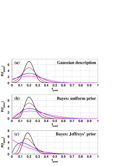
FIG. 2.: Different posterior pdfs from sample sizes of 5, 10, 20, and 50 events are shown. Plot (a) shows normally distributed pdfs; only points within the physical region are shown. Plot (b) shows Bayesian posterior pdfs when a uniform distribution is used as the prior. The pdfs of (a) and (b) each have a most likely value of $f_{pass}=0.2$. Plot (c) shows Bayesian posterior pdfs when Jeffreys’ prior is used, where the fraction of events that pass the cut is 0.2 for each pdf. No part of any pdf in (b) or (c) extends beyond the physical region $0\leq f_{pass}\leq 1$.

Several authors [2] [3] have used the following posterior pdf to describe $P(f_{pass})$ in the interval $0\leq f_{0}\leq 1$:

$$P(f_{pass};N_{pass},N_{Total})=\frac{(N_{Total}+1)\>!}{N_{pass}\>!\;(N_{Total}-N_{pass})\>!}\>{\left(f_{pass}\right)}^{N_{pass}}\>{\left(1-f_{pass}\right)}^{N_{Total}-N_{pass}}\;.$$ (49)

The most likely value for this posterior is simply the fraction of events that pass the cut, $f_{0}=N_{pass}/N_{Total}$. Figure 2b shows Equation 49 for different values of $N_{Total}$, each with the same most likely value of $f_{0}=0.2$. The origin of this posterior is the use of a uniform prior over the physical region,

$$P(f_{pass})=\left\{\begin{array}[]{rl}1&\mbox{if $0\leq f_{pass}\leq 1$}\\ 0&\mbox{otherwise}\end{array}\right.\;.$$ (50)

The experimental likelihood is the binomial distribution,

$$P(f_{pass})=\frac{N_{Total}\>!}{N_{pass}\>!\;(N_{Total}-N_{pass})\>!}\>{\left(f_{pass}\right)}^{N_{pass}}\>{\left(1-f_{pass}\right)}^{N_{Total}-N_{pass}}\;.$$ (51)

The evidence, or marginalization term, normalizes the posterior to unit area, and is found by integration:

$$\mbox{evidence}=\int_{-\infty}^{+\infty}\left(\mbox{prior}\times\mbox{experimental likelihood}\right)df_{pass}\;.$$ (52)

In the case of the uniform prior, the evidence term for this experimental likelihood distribution is equal to ${(N_{Total}+1)}^{-1}$.

It is possible to construct a different posterior pdf $P(f_{pass})$ with a different choice of prior, e.g.,

$$P(f_{pass};N_{pass},N_{Total})=\frac{N_{Total}\>!}{(N_{pass}-1)\>!\;(N_{Total}-N_{pass})\>!}\>{\left(f_{pass}\right)}^{N_{pass}-1}\>{\left(1-f_{pass}\right)}^{N_{Total}-N_{pass}}$$ (53)

arises if Jeffreys’ (divergent) prior is used:

$$P(f_{pass})=\left\{\begin{array}[]{cl}1/f_{pass}&\mbox{if $0<f_{pass}\leq 1$}\\ 0&\mbox{otherwise}\end{array}\right.\;.$$ (54)

The evidence term in this case is equal to ${(N_{pass})}^{-1}$. The most likely value of Equation 53 is $f_{0}=(N_{pass}-1)/(N_{Total}-1)$, which approximates the most likely values of Equations 48 and 49 as for large sample sizes. Figure 2c shows the evolution of Equation 53 as the sample size is increased while the fraction of events that pass the cut is held constant.

The posterior pdf of Equation 53 is included for completeness and will not be used in this solution to the measurement problem. Notice that the use of a divergent prior excludes cases of $N_{pass}=0$. Jeffreys’ prior would be used in those cases when an experimentalist claims complete ignorance of the efficiency of the cut in the absence of any surviving events; i.e., if zero events pass the cut, the experimentalist who favors Jeffreys’ prior will not claim that any event will ever pass the cut. This is obviously not satisfactory when attempting to set upper limits on a data sample with zero surviving events. In such a case, if the experimentalist is comfortable with setting the most likely value of the posterior $P(f_{pass})$ at $f_{0}=0$ when $N_{pass}=0$, a flat prior should be used.

The three different posteriors, Equations 48, 49 and 53, demonstrate a feature of BPT; as the sample size increases the posterior pdf becomes less sensitive to the particular choice of the prior pdf. Furthermore, as long as the most likely value of the distribution is not too close to its limiting values, as the sample size increases, the Gaussian distribution more closely approximates the posterior pdfs of Equations 49 and 53. Figure 3a shows the three different posteriors in the case of small sample size; Figure 3b shows the same distributions from a twenty times larger sample.

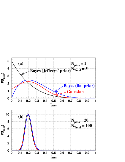
FIG. 3.: The three different posterior pdfs for a sample of events where 20% of the events pass the cut. Plot (a) shows the posteriors for a sample size of five events. Plot (b) shows the posteriors for a sample size of 100 events.

In this paper the notation $P(x)$ represents a pdf of no particular form. For complete generality, the pdfs for the efficiencies $\varepsilon$ and $r$ will be written as $P(\varepsilon)$ and $P(r)$; it should be assumed that for the remainder of this paper each is a shorthand representation for a binomial posterior described by Equation 49. For other cases, the notation $P(x;x_{pass},x_{Total})$ will be used to describe a binomial posterior of the form given by Equation 49, while $P(x;x_{0},\sigma_{x})$ describes an explicitly Gaussian pdf of the form given by Equation 48. Even though the posterior pdf represents the complete knowledge of the particular distribution of possible values of a measured quantity, it is common to summarize the results of an experiment, i.e. the posterior, with only a few numbers. Typically an experimental result will be quoted as the most likely value (the mode of the posterior) with an upper and lower limit such that the most likely value is contained within the limits at some confidence level. For multi-modal posteriors it may be more appealing to quote the mean of the posterior rather than the modal value. Binomial problems do not of themselves give rise to multimodal posteriors. For the purposes of this paper, the most likely value of a posterior will be quoted; the most likely value of a posterior $P(x)$ will be represented $x_{0}$. When error bars for a confidence level $\alpha$ are quoted, they describe the shortest interval about the most likely value that contains area $\alpha$ beneath the posterior pdf. Figure 4 shows the $\alpha=0.683$ and $\alpha=0.955$ confidence intervals for a Bayesian posterior constructed by Equation 49.

FIG. 4.: The Bayesian posterior pdfs (uniform prior) for a sample of 10 events of which 2 events passed the cut. The hatched region of plot (a) represents the 0.683 confidence level interval about the most likely value of $f_{pass}=0.2$. The hatched region of plot (b) represents the 0.955 confidence level interval about the most likely value of $f_{pass}=0.2$. Also shown is the equivalence of these confidence intervals and those defined by differences in the log-likelihood $\ln P(f_{pass})$.

IV A solution for the measurement problem

In Section III it was shown that BPT can be used in binomial problems to construct posterior pdfs that exist completely within the allowed physical region. The application of cuts to finite data sets is a binomial problem: events in a data sample will either pass or fail a particular cut. While this classification is completely natural during the course of an experiment, the binomial quantity of interest is not the fraction of events which pass a cut, but the fraction of signal events in the original sample. A useful theorem of BPT provides a means of constructing a physical posterior pdf $P(f_{sig}$) from the experimental posterior pdf $P(f_{pass})$.

Generally, if a variable $y$ is a function of variable $x$, $y=f(x)$, an existing posterior distribution $P(y)$ can be used to construct a desired posterior function $P(x)$ simply by replacing $y$ in $P(y)$ with the functional form of $x$ and multiplying this posterior by the Jacobian [4]:

$$P(x)=P\bigl{(}y(x)\bigr{)}\times\left|\frac{dy}{dx}\right|.$$ (55)

In the measurement problem, this change of variables takes the form:

$$P(f_{sig})=P\bigl{(}f_{pass}(f_{sig})\bigr{)}\times\left|\frac{df_{pass}}{df_{sig}}\right|,$$ (56)

so that

$$P(f_{sig};\varepsilon,r,N_{pass},N_{Total})=P\bigl{(}(\varepsilon-r)f_{sig}+r;N_{pass},N_{Total}\bigr{)}\times|\varepsilon-r|\;.$$ (57)

When Equations 49 and 37 are used, the posterior pdf that describes the amount of signal in the original sample is:

$$P(f_{sig};\varepsilon,r,N_{pass},N_{Total}) = \frac{|\varepsilon-r|\>(N_{Total}+1)\>!}{N_{pass}!\;(N_{Total}-N_{pass})\>!}\times$$ (59)

$${\Bigl{(}(\varepsilon-r)f_{sig}+r\Bigr{)}}^{N_{pass}}\>{\Bigl{(}1-\bigl{(}(\varepsilon-r)f_{sig}+r\bigr{)}\Bigr{)}}^{N_{Total}-N_{pass}}\;.$$

The efficiency $\varepsilon$ and the rfficiency $r$ should be considered nuisance parameters as posterior pdfs $P(\varepsilon)$ and $P(r)$ can be constructed, according to Equation 49 in Section III, from independent control samples. Once these posteriors are known, e.g. $P(\varepsilon;\varepsilon_{pass},\varepsilon_{Total})$, the nuisance parameters can be integrated away:

$$P(f_{sig};N_{pass},N_{Total})=\int_{0}^{1}d\varepsilon\int_{0}^{1}dr\;P(\varepsilon)\;P(r)\;P\left(f_{sig};\varepsilon,r,N_{pass},N_{Total}\right)\;.$$ (60)

Equation 60 is the solution to the measurement problem. The efficiency $\varepsilon$, the rfficiency $r$, the size of the sample $N_{Total}$, and the number of events which pass the cut $N_{pass}$ all contribute to the posterior pdf for the fraction of the signal events in the original sample. This posterior is completely Bayesian: it will provide a most likely value for the signal fraction; it also allows for the natural construction of confidence intervals. Alternately, Equation 60 could be written in terms of $P(f_{bkg})$, because of the trivial relationship $f_{sig}+f_{bkg}=1$.

This method of constructing $P(f_{sig};N_{pass},N_{Total})$ from Equation 60 allows the state-of-knowledge of $\varepsilon$ and $r$ to enter the understanding of $f_{sig}$ in a natural way. The efficiency and rfficiency originate from independent control samples; their most likely values depend on the particular cut used. It may be the case that $\varepsilon$ and $r$ have modal values $\varepsilon_{0}$, $r_{0}$ which lead to a measurement matrix with a small condition number, q.v. Equation 46, but that they are found from such small diagnostic samples that the posterior pdfs $P(\varepsilon)$, $P(r)$ are very broad. This will lead to a broader distribution for $P(f_{sig})$ than the case of very precisely known $\varepsilon$ and $r$. Often experimentalists face the dilemma of diverting bandwidth from the recording of possible signal sources to the task of increasing the size of control samples, especially when suffering from limited statistics in one or more control samples. Equation 60 introduces an easy way to evaluate control samples of different sizes. See Example 2 below.

It should be noted that even in cases where $\varepsilon$ and $r$ are known very precisely, small sample sizes may lead to a pdf $P(f_{pass})$ which has non-zero values outside the physical region $r\leq f_{pass}\leq\varepsilon$.  In such cases, the integral of $P(f_{sig})$ over the physically allowed values $0\leq f_{sig}\leq 1$ will be less than unity. It is useful to define an overall confidence level for the experiment,

$$\alpha_{experiment}\equiv\int_{0}^{1}P(f_{sig};N_{pass},N_{Total})\;df_{sig}\;.$$ (61)

The value $\alpha_{experiment}$ is the confidence that the observed values of $N_{pass}$ and $N_{Total}$ are consistent with the knowledge $P(\varepsilon)$ and $P(r)$. Equation 61 also defines the maximum confidence level that can be quoted for the posterior pdf $P(f_{sig})$. Since $P(f_{sig})$ is restricted to $0\leq f_{sig}\leq 1$, $(1-\alpha_{experiment})$ is the fraction of the posterior that could not be constructed because part of $P(f_{sig})$ lies beyond the physical boundaries. Recall that by the construction of Equation 49,

$$\int_{0}^{1}P(f_{pass};N_{pass},N_{Total})\;df_{pass}=1\;.$$ (62)

While the Bayesian posterior pdf $P(f_{pass})$ is normalized to unity, representing complete certainty that the fraction of events which pass a cut is between zero and one, the posterior pdf $P(f_{sig})$ is not normalized, except by the Jacobian as seen in Equation 55. A case of $\alpha_{experiment}$ less than one simply implies that larger data and/or diagnostic samples are required to increase the confidence that $f_{sig}$ is within the expected physical region. In cases where either $\varepsilon$ or $r$ are imprecisely known, the overall confidence of the experiment may be small if the fraction of events which pass the cut is very close to either $\varepsilon_{0}$ or $r_{0}$. In the event of an overall experimental confidence level of much less than one, the experimentalist is encouraged to alter the cut such that $f_{pass}$ is not too close to either $\varepsilon$ or $r$, or to increase the sample size $N_{Total}$.

Figure 4 shows the equivalence of Bayesian confidence level intervals and those constructed by differences in the log of the posterior [5]. In cases of $\alpha_{experiment}=1$, the posterior is zero for all values outside the physical region: here the log-likelihood method will always provide an interval completely within the physical region. In the case of $\alpha_{experiment}<1$, the log-likelihood method may not be able to set one or both limits within the physical region. See the insert of Figure 5b for Example 1 below for an example of an experiment that could not set bounds with a confidence level of greater than 93%.

It should be noted that if for some reason the posteriors $P(\varepsilon)$ or $P(r)$ are constructed by some formalism other than that of Section III which causes one or both of them to be multimodal, the posterior $P(f_{sig})$ may become multimodal. This would be a very unlikely circumstance that arises only through the drastic intervention on the part of the experimenter.

This solution to the measurement problem presents the results as a fraction of signal events $f_{sig}$ in the original sample of $N_{Total}$ events. It may be preferrable for certain calculations, such as cross section measurements, to find the total number of signal events $N_{sig}$. It is trivial to use Equation 29 to perform the change of variables described by Equation 55:

$$P(N_{sig})=P\left(\frac{N_{sig}}{N_{Total}};N_{pass},N_{Total}\right)\left|\frac{1}{N_{Total}}\right|.$$ (63)

The posterior $P(N_{sig})$ is defined on the interval $0\leq N_{sig}\leq N_{Total}$.

Equation 60 is not only a useful method for interpreting the results a single experiment, but it can also be used as an unbiased tool to evaluate the possibility of applying different sets of cuts to the same original data sample, see Example 1 below. This method has the further ability to quickly judge the possible improvements in a result from increased sample sizes, both for the data and control samples. Possible improvements may take the form of a larger value of $\alpha_{experiment}$, a shorter confidence level interval about the most likely value of $f_{sig}$, or both.

V The measurement of signal in a subsample

If an experiment is designed to extract a signal-rich sample of events by applying a cut, it is unusual to quote the fraction of signal events in the original sample that may be dominated by background events. Rather than quoting the signal fraction from the $N_{Total}$ event sample, it may be more useful to quote either the signal fraction or the number of signal events in the subsample of $S_{pass}$ events that pass the cut. Recall that the equation for $S_{pass}$ is, from Equations 7 and 24,

$$S_{pass} = \left(\frac{\varepsilon}{\varepsilon-r}\right)\left(N_{pass}-r\cdot N_{Total}\right)$$ (64)

$$= \left(\frac{\varepsilon\cdot N_{pass}}{\varepsilon-r}\right)\left(1-\frac{r}{f_{pass}}\right)\;.$$ (65)

Rearranging the above, $f_{pass}$ can expressed as a function of $S_{pass}$:

$$f_{pass}=\frac{\varepsilon\cdot r\cdot N_{pass}}{\varepsilon\cdot N_{pass}-(\varepsilon-r)S_{pass}}\;.$$ (66)

The number of signal events in the sample of events which passed the cut is restricted to the interval $0\leq S_{pass}\leq N_{pass}$. As in Section IV, a posterior describing some fraction of events $g$ will be used so that $0\leq g\leq 1$. The definition of $g$ for this problem is

$$g\equiv\frac{S_{pass}}{N_{pass}}\;.$$ (67)

Equation 66 is used to express $f_{pass}$ as a function of $g$:

$$f_{pass}=\frac{\varepsilon\cdot r}{\varepsilon-(\varepsilon-r)g}\;.$$ (68)

Just as it was possible to change variables in order to construct a posterior pdf $P(f_{sig})$ from the form of the posterior for $P(f_{pass})$, it is possible to construct of $P(g)$. The Jacobian from Equation 68 is

$$\left|\frac{df_{pass}}{dg}\right|=\left|\frac{\varepsilon\cdot r\>(\varepsilon-r)}{{\bigl{(}\varepsilon-(\varepsilon-r)g\bigr{)}}^{2}}\right|\;.$$ (69)

The posterior pdf $P(g)$ is then

$$P(g;\varepsilon,r,N_{pass},N_{Total})=P\biggl{(}\Bigl{(}\frac{\varepsilon\cdot r}{\varepsilon-(\varepsilon-r)g}\Bigr{)};N_{pass},N_{Total}\biggr{)}\times\left|\frac{\varepsilon\cdot r\>(\varepsilon-r)}{{\bigl{(}\varepsilon-(\varepsilon-r)g\bigr{)}}^{2}}\right|\;.$$ (70)

As before, the nuisance parameters $\varepsilon$ and $r$ should be integrated away:

$$P(g;N_{pass},N_{Total})=\int_{0}^{1}d\varepsilon\int_{0}^{1}dr\;P(\varepsilon)\;P(r)\;P\left(g;\varepsilon,r,N_{pass},N_{Total}\right)\;.$$ (71)

Equation 71 can be converted into a posterior for $S_{pass}$ if a change-of-variables similar to that of Equation 63 is performed, so

$$P(S_{pass};N_{pass},N_{Total})=\int_{0}^{1}d\varepsilon\int_{0}^{1}dr\;{(N_{pass})}^{-1}\;P(\varepsilon)\;P(r)\;P\left(g;\varepsilon,r,N_{pass},N_{Total}\right)\;.$$ (72)

The posterior of Equation 72 is defined for the interval $0\leq S_{pass}\leq N_{pass}$. Similar posteriors can be constructed to describe $S_{fail}$, $B_{pass}$, or $B_{fail}$.

Example 1: The discovery of the top quark

In 1995 the CDF [6] and DØ [7] collaborations reported conclusive evidence for the process $p\overline{p}\rightarrow t\overline{t}+X$ production at the Fermilab Tevatron. The key to this discovery was the ability of each experiment to devise cuts for the efficient selection of $t\overline{t}$ signal events from a parent sample of events with a high transverse momentum lepton (from the decay of a $W^{\pm}$ boson) and three or more jets. This important discovery can be used to illustrate the use of Equation 60.

The CDF experiment claimed discovery with 67 $\mbox{pb}^{-1}$ of integrated luminosity using analyses based on two different methods of discriminating signal from background through the identification of $b$ jets. The first method (SVX tag) identified $b$ jets by the reconstruction of secondary vertices within a silicon vertex detector. The second method (SLT tag) involved the reconstruction of soft leptons (here, electrons or muons) from the semileptonic decay of $b$ quarks. As expected these two methods had different efficiencies for both the signal and background, and different numbers of events passed each cut.

Table I contains the relevant information as published by the CDF experiment. Also included is the CDF result [8] using SVX tags from a Run 1 data set corresponding to 109 $\mbox{pb}^{-1}$ of integrated luminosity. Even though the SVX and SLT methods have very different efficiencies, the different methods show good agreement in the fraction of signal events in the original sample of 203 $W^{\pm}+3$ (or more) jets events. Notice the agreement between the measured number of signal events $S_{pass}$ from Equation 72 and the reported CDF numbers.

TABLE I.: The discovery of the top quark at the CDF experiment: Shown are the results of the solution to the measurement problem as applied to the published values of $\varepsilon$ and $r$. Compare the solution’s $S_{pass}$ to the published CDF value. Also shown are the CDF results from a Run 1 data set corresponding to a larger integrated luminosity of 109 $\mbox{pb}^{-1}$.

	$N_{Total}$	$N_{pass}$	$\varepsilon$ (%)	$r$ (%)	$f_{sig}$	$S_{pass}$	$\alpha_{exp}$	CDF
SVX (67 $\mbox{pb}^{-1}$)	203	27	$42\pm 5$	$3.3\pm 0.1$	$0.25^{+0.08}_{-0.07}$	$22.5^{+2.3}_{-1.9}$	1.0	$20.3\pm 2.1$
SLT (67 $\mbox{pb}^{-1}$)	203	23	$20\pm 2$	$7.6\pm 0.1$	$0.24^{+0.22}_{-0.18}$	$13.2^{+4.6}_{-6.0}$	0.93	$7.6\pm 2.0$
SVX (109 $\mbox{pb}^{-1}$)	322	34	$42\pm 5$	$3.3\pm 0.1$	$0.18^{+0.06}_{-0.05}$	$26.0^{+2.3}_{-2.7}$	1.0	$25.5\pm 1.7$

Figure 5 shows the state-of-knowledge of the efficiencies for signal and background, as well as the knowledge of the fraction of events which survive the different $b$-tag requirements. In Figure 5a it is easy to see how the well-separated pdfs $P(r)$, $P(\varepsilon)$, and $P(f_{pass})$ of the SVX measurement give rise to a more precise measurement of $f_{sig}$. The overlapping pdfs of the SLT measurement shown in Figure 5b return a similar most-likely value of $f_{sig}$, but the overall precision of the SLT measurement is worse. The poor separation of the pdfs in the SLT measurement leads to an overall experimental confidence level of 93%, compared to the 100% confidence of the SVX measurement. This can be seen graphically by comparing the inserts of Figure 5: The SVX result is completely within the physical region $0\leq f_{sig}\leq 1$, while 7% of $P(f_{sig})$ for the SLT result lies outside the physical region.

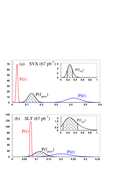
FIG. 5.: The probability density functions of interest for CDF’s top quark discovery for the (a) SVX-tag sample, and (b) SLT-tag sample. The inserts show the measured fraction of signal events in the entire data sample; the hatched regions show the 0.683 CL interval about the most likely value of $f_{sig}$. Notice that the overlapping pdfs of (b) cause a less precise measurement of $f_{sig}$.

Example 2: Using $W^{\pm}(\rightarrow e^{\pm}\nu)$ production as a luminosity monitor at Tevatron Run 2

It has been suggested [9] that the two major Tevatron collider experiments count the number of events from the process $p\overline{p}\rightarrow W^{\pm}(\rightarrow e^{\pm}\nu)+X$ during Tevatron Run 2 and use the theoretical predictions for the cross section times branching ratio ($\sigma_{signal}$) to measure the integrated luminosity (${\cal L}$). It is hoped that such a ‘$W$ counting’ method can measure the integrated luminosity recorded at each experiment more precisely than the approximately 4% precision [9] [10] used in the Run 1 physics results:

$${\cal L}=\frac{S_{pass}}{\varepsilon\cdot A\cdot\sigma_{signal}}\;.$$ (73)

The variables $S_{pass}$ and $\varepsilon$ have the same definitions as in Section II; $A$ represents the kinematic and geometric acceptance of the detector used to collect the signal events. It is more natural to reformulate Equation 73 in terms of the total number of signal events recorded,

$${\cal L}=\frac{N_{sig}}{A\cdot\sigma_{signal}}\>,$$ (74)

so that the measured fraction of signal events is a function of the integrated luminosity:

$$f_{sig}=\frac{N_{sig}}{N_{Total}}=\frac{{\cal L}\cdot A\cdot\sigma_{signal}}{N_{Total}}\>.$$ (75)

Following the derivation of Equation 63:

$$P({\cal L})=P\left(\frac{{\cal L}\cdot A\cdot\sigma_{signal}}{N_{Total}};N_{pass},N_{Total}\right)\left|\frac{A\cdot\sigma_{signal}}{N_{Total}}\right|.$$ (76)

The posterior $P({\cal L})$ is defined on the interval $0\leq{\cal L}\leq{\cal L}_{max}$, where

$${\cal L}_{max}=\frac{N_{Total}}{A\cdot\sigma_{signal}}\;.$$ (77)

The variables of Equation 76 are: the number of total events ($N_{Total}$) prior to a selection of signal events ($N_{pass}$) by a cut with some efficiency ($\varepsilon$) and rfficiency ($r$); the acceptance of the detector ($A$); and the theoretical cross section times branching fraction ($\sigma_{signal}$). It will be assumed that the acceptance of a given detector can be known to an arbitrarily small precision through the use of large Monte Carlo data sets and a complete detector simulation, i.e.:

$$P(A)=\left\{\begin{array}[]{rl}1&\mbox{if $A=A_{0}$}\\ 0&\mbox{otherwise}\end{array}\right.\;.$$ (78)

The knowledge of the efficiency of the selection criteria, $P(\varepsilon)$, will come from $Z^{0}\rightarrow e^{+}e^{-}$ decays recorded during data taking; for Tevatron Run 2 the size of this sample will be twenty times the approximately five thousand such events recorded during Run 1 [10].

Ignoring the uncertainty in the integrated luminosity, the background fraction in the sample of events which pass the cuts ($r\times f_{bkg}$) was the dominant source of uncertainty in the measured $p\overline{p}\rightarrow W^{\pm}(\rightarrow e^{\pm}\nu)+X$ cross sections from Run 1. It is impossible to predict the exact amount of background that a given experiment will have prior to data collection, so the most important experimental question facing an experiment that wishes to use a process like inclusive $W^{\pm}$ production is: How much diagnostic data is needed to understand the background to an arbitrary degree of accuracy?

In order to perform such a study, it is necessary to assume that each Tevatron experiment will be delivered 2 $\mbox{fb}^{-1}$ of data, and that $\varepsilon$, $r$, and $A$ will be close to the currently reported values from Run 1. It will be assumed that there is no uncertainty in the theoretical cross section times branching ratio $\sigma_{signal}$; the value of the reported DØ measurement [10] will be used for $\sigma_{signal}$. The size of the total data sample $N_{Total}$ will be the sum of the number of signal events ($N_{sig}$) and an arbitrary number of background events ($N_{bkg}$) depending on the value of $r\times f_{bkg}$:

$$N_{bkg}=\left(r\times f_{bkg}\right)\frac{N_{sig}}{1-(r\times f_{bkg})}\;.$$ (79)

TABLE II.: The assumed values for the Tevatron Run 2 $p\overline{p}\rightarrow W^{\pm}(\rightarrow e^{\pm}\nu)+X$ cross section measurement at DØ . The measured value of the Run 1b inclusive $W^{\pm}$ boson production cross section times branching ratio from the DØ experiment is used in place of a theoretical value for $\sigma_{signal}$. The value of $\varepsilon_{Total}$ is an estimate of the total number of $Z^{0}\rightarrow e^{+}e^{-}$ events that will available for the measurement of the efficiency.

Experiment	$r_{0}$	$\varepsilon_{0}$	$\varepsilon_{Total}$	${\cal L}$	$A_{0}$	$\sigma_{signal}$
DØ	0.43	0.70	108 000	2 $\mbox{fb}^{-1}$	0.465	2310 pb

Table II lists the assumed values for the Run 2 $W^{\pm}(\rightarrow e^{\pm}\nu)$ cross section measurement for the DØ experiment. Table III shows the $1\sigma$ confidence limit in the measured integrated luminosity that can be expected for a given experiment for different control sample sizes ($r_{Total}$). The QCD background fraction in the inclusive $W^{\pm}$ sample is known to vary with instantaneous luminosity and trigger definitions [10] [11]; Table III shows the effect of different amounts of background on the precision of the luminosity measurement. Note that the figures for the DØ experiment assume that both the central (CC) and endcap (EC) calorimeters are used; if only the CC is used the DØ experiment can expect a more precise measurement of integrated luminosity since the background fractions in the central region should be approximately one-fifth the value in the EC regions, even though 70% of the acceptance for $W^{\pm}\rightarrow e^{\pm}\nu$ events is in DØ’s central region.

It should be noted that the upgraded DØ central tracker to be used in Run 2 will almost certainly have different values of $\varepsilon_{0}$ and $r_{0}$ than used here. Nevertheless, Table III shows that even with moderately sized diagnostic samples (one-tenth the size of the final $Z^{0}\rightarrow e^{+}e^{-}$ sample) it should be possible to measure the integrated luminosity to a precision of better than 1% with this method, assuming that the theoretical uncertainties can be kept at or below this level of precision.

TABLE III.: Shown are the $1\sigma$ confidence level intervals about the nominal Tevatron Run 2 integrated luminosity ${\cal L}_{0}=2\;\mbox{fb}^{-1}$, as a function of the amount of background and the number of diagnostic events available to measure $P(r)$.

Experiment	$r_{0}\times f_{bkg}$	$r_{Total}$	$1\sigma$ interval about ${\cal L}_{0}$
DØ (nominal bkg)	0.064	1 000	$\pm\;0.017\;\mbox{fb}^{-1}$
DØ (nominal bkg)	0.064	10 000	$\pm\;0.012\;\mbox{fb}^{-1}$
DØ (nominal bkg)	0.064	100 000	$\pm\;0.011\;\mbox{fb}^{-1}$
DØ (less bkg)	0.030	1 000	$\pm\;0.013\;\mbox{fb}^{-1}$
DØ (less bkg)	0.030	10 000	$\pm\;0.012\;\mbox{fb}^{-1}$
DØ (less bkg)	0.030	100 000	$\pm\;0.011\;\mbox{fb}^{-1}$
DØ (more bkg)	0.100	1 000	$\pm\;0.026\;\mbox{fb}^{-1}$
DØ (more bkg)	0.100	10 000	$\pm\;0.012\;\mbox{fb}^{-1}$
DØ (more bkg)	0.100	100 000	$\pm\;0.010\;\mbox{fb}^{-1}$

VI The Confidence Level for the Possible Discovery of a Signal

It may be the case that an experiment provides a sample of $N_{Total}$ events, and the expected number of events $\mu_{B}$ is modeled by a some pdf, e.g. $P(\mu_{B};B,\sigma_{B})$, where the most likely value $B$ is less than the observed number of events. In such a case, the experimentalist may believe that the excess, $N_{Total}-B$, is due to a real signal rather than a statistical fluctuation. The confidence level $\alpha_{excess}$ that the excess is due to something beyond the expected background can be defined [12] as

$$\alpha_{excess}\equiv 1-\!\!\sum_{N=N_{Total}}^{\infty}\int_{0}^{\infty}d\mu_{B}\;\frac{e^{-\mu_{B}}\>\mu_{B}^{N}}{N!}\;P(\mu_{B})\;,$$ (80)

or

$$\alpha_{excess}\equiv\sum_{N=0}^{N_{Total}-1}\int_{0}^{\infty}d\mu_{B}\;\frac{e^{-\mu_{B}}\>\mu_{B}^{N}}{N!}\;P(\mu_{B})\;.$$ (81)

In the case of an excess, it should be assumed that $P(\mu_{B})=0$ for all $\mu_{B}>N_{Total}$, so Equation 81 can be written

$$\alpha_{excess}\equiv\sum_{N=0}^{N_{Total}-1}\int_{0}^{N_{Total}}d\mu_{B}\;\frac{e^{-\mu_{B}}\>\mu_{B}^{N}}{N!}\;P(\mu_{B})\;.$$ (82)

It is natural to try to enhance the significance of a possible signal by reducing the expected background $\mu_{B}$. This is done by applying a cut on the sample of $N_{Total}$ events. A cut is usually chosen such that the rfficiency of the cut on the background events (here, the anticipated events described by $P(\mu_{B})$ ) is small, while the expected efficiency of the cut on the possible signal is large. Equation 24 can be turned around;

$$\varepsilon\cdot N_{sig}=N_{pass}-r\cdot N_{bkg}\;.$$ (83)

In order to claim a positive signal, there are two conditions. The trivial condition is that the efficiency $\varepsilon$ is non-zero. The more important condition is that $N_{pass}>r\cdot N_{bkg}$. If there is an excess, the significance of the excess in the sample of $N_{pass}$ events incorporates the knowledge of $r$ and $\mu_{B}$ through the pdfs $P(r)$ and $P(\mu_{B})$:

$$\alpha_{discovery}\equiv\sum_{N=0}^{N_{pass}-1}\int_{0}^{1}dr\int_{0}^{N_{Total}}d\mu_{B}\;\frac{e^{-(r\cdot\mu_{B})}\>{(r\cdot\mu_{B})}^{N}}{N!}\;P(\mu_{B})\;P(r)\;.$$ (84)

$N_{pass}^{disc}$ can be defined as the minimum number of events $N_{pass}$ from Equation 84 that guarantees a confidence level $\alpha_{discovery}$ in the signal. Just as in Equation 60, the knowledge of the rfficiency $P(r)$ plays a critical part in the solution to this problem. The attempt to enhance a possible signal is a common exercise that is often fraught with difficulties; Equation 84 is an unbiased tool to estimate the minimum number of events which must survive any new cut used to extract a possible signal.

Example 3: Discovery of a Higgs boson at CDF?

In 1997 the CDF experiment [13] reported a slight excess of events in the process $p\overline{p}\rightarrow W^{\pm}+2$ jet events in events where the $W^{\pm}$ boson decayed to either an electron or muon, and one of the jets in the event was identified as coming from a $b$ quark decay by either the SVX or SLT tagging method. The CDF data is summarized in Table IV.

TABLE IV.: The CDF results reporting a possible excess of observed $W^{\pm}+2$ jets sample where one or both of the jets has been $b$-tagged. The significance of the excess ($\alpha_{excess}$) has been calculated using a Gaussian distribution with mean $B$ and width $\sigma_{B}$.

Sample	Number Observed	Background Estimate ($B\pm\sigma_{B}$)	$\alpha_{excess}$
$W^{\pm}$ + 2 jets (no tag)	1527	-	-
$W^{\pm}$ + 2 jets (one tag)	36	$30\pm 5$	0.49
$W^{\pm}$ + 2 jets (both tagged)	6	$3.0\pm 0.6$	0.90

An interesting but yet unobserved Standard Model process that has the experimental signature of a $W^{\pm}$ boson and two $b$-jets is associated production of $W^{\pm}$ boson and a Higgs boson [14], i.e. $p\overline{p}\rightarrow W^{\pm}+H^{0}$. It is reasonable to try and enhance the 49% confidence level excess in the CDF single-tag sample by requiring both jets to be tagged; Table IV shows that this requirement increases the confidence that the excess is due to a signal beyond expectations to 90%. Based on the CDF results, it is possible to estimate how many events would pass the double-tag requirement in order to claim a higher significance. From the data shown in Table IV it can be assumed that the rfficiency of the double-tag requirement is to be 10%. Table V shows the minimum number of events from the single-tag sample that would have to pass the double-tag requirement in order to claim excesses at the $2\sigma$ and $3\sigma$ levels. Also shown is the case where only 5 events pass the double-tag rquirement, which has an $\alpha_{excess}$ confidence level of only $1\sigma$.

TABLE V.: Shown are the minimum number of events $N_{pass}^{disc}$ that must pass a cut in order to claim discovery of a signal at a given confidence level $\alpha_{discovery}$, for Example 3.

$N_{Total}$	$B$	$\sigma_{B}$	$r_{pass}$	$r_{Total}$	$\alpha_{discovery}$	$N_{pass}^{disc}$
36	30	5	10	100	0.683	5
36	30	5	10	100	0.955	8
36	30	5	10	100	0.997	11

VII Crosschecks for the possible discovery of a signal

If after the application of the cut a significant excess is observed, it is straightforward to use the measurement problem as a cross check of the possible discovery. In order to perform such a cross check, some knowledge $P(\varepsilon)$ of the efficiency $\varepsilon$ of the cut on the (possible) signal is necessary. If nothing is known about $\varepsilon$ except that it was large enough to provide discovery, i.e. $\varepsilon>r$, the uniform pdf prior to be used for $P(\varepsilon)$ is

$$P(\varepsilon)=\left\{\begin{array}[]{cl}0&\mbox{when $\varepsilon\leq r$}\\ {(1-r)}^{-1}&\mbox{when $\varepsilon>r$}\end{array}\right.\;.$$ (85)

Otherwise, if there is some a priori knowledge assumed about the possible signal, there may be more informed knowledge of $\varepsilon$, perhaps from a Monte Carlo simulation. With the knowledge of the efficiency and the rfficiency for the cut, it is reasonable to assess the overall confidence that fewer than $N_{fail}^{disc}$ events will fail the cut, where $N_{fail}^{disc}$ is the number of events which are removed from the sample by a cut designed to enhance the possible signal. The expected number of events that will fail the cut $\mu_{fail}$ is

$$\mu_{fail}=(1-\varepsilon)\;N_{Total}+(\varepsilon-r)\;\mu_{B}\;.$$ (86)

Recall that for a possible discovery $\varepsilon>r$, so $\mu_{fail}$ will never be negative. It is important to recognize that from the substitution of $N_{pass}^{disc}=N_{Total}-N_{fail}^{disc}$ into Equation 84, a small value of $N_{fail}^{disc}$ which leads to large value of $\alpha_{discovery}$ may be inconsistent with the original description of the expected background.

The confidence level $\beta$ that fewer than $N_{fail}$ events will fail the new cut given the expected background $\mu_{B}$ is

$$\beta=\sum_{N=0}^{N_{fail}}\int_{0}^{1}dr\int_{0}^{N_{Total}}d\mu_{B}\int_{0}^{1}d\varepsilon\;\frac{e^{-\mu_{fail}}\>\mu_{fail}^{N}}{N!}\;P(\varepsilon)\;P(\mu_{B})\;P(r)\;.$$ (87)

The variable $\beta$ is used here because in cases where the efficiency and rfficiency are known very precisely, $\beta$ expresses the confidence that the initial description of the background distribution can still accommodate the new excess. In other words, $\beta$ is a measure of how likely it is for $N_{pass}$ (or more) events to remain after the application of the new cut, given the assumption that the original sample of events contains both a new signal and the expected background.

Notice that once $N_{Total}$ is fixed, the number of events $N_{pass}^{disc}$ necessary to claim a discovery with a confidence level $\alpha_{discovery}$ is a function of $r$ and $\mu_{B}$ only. Once a discovery is claimed, the confidence level $\beta$ in the original background description depends not only on $r$ and $\mu_{B}$, but also $\varepsilon$. This reflects the fact that the efficiency $\varepsilon$ of a cut has no meaning for a sample devoid of signal events. In the limiting case of Equation 87 where both $\varepsilon$ and $r$ approach unity with complete certainty, $N_{fail}$ approaches zero and $\beta$ approaches an upper limit of 1; if no further cut is placed on the sample, there is complete confidence that the original background description accomodates the observed excess. A value of $\beta\approx 1$ implies that $P(\mu_{B})$ can completely accommodate an excess in $N_{pass}$; $\beta\approx 0$ implies that the description of the background cannot accommodate such an excess.

Example 4: The degree-of-belief for a Run 1 Higgs discovery

The CDF data used in Example 3 is a case where a double $b$-tag sample of $W^{\pm}$ + 2 jet events shows an excess of observed events over expectations at the 90% level, see Table IV. For simplicity, and to insure that the mathematical description of the number of background events never has a value greater than the observed number of events, the distribution of expected events $P(\mu_{B})$ will be modeled here as

$$P(\mu_{B})=\left\{\begin{array}[]{cl}({2\>\sigma_{B}})^{-1}&\mbox{if $B-\sigma_{B}\leq\mu_{B}\leq B+\sigma_{B}$}\\ 0&\mbox{otherwise}\end{array}\right.\;.$$ (88)

This model for the background lowers the significance of the excess in the double-tag sample from 90% to 87%, but it will serve as an approximation to a Gaussian description of the expected background. Three different cases will be considered for the possible new signal that is causing the excess in the double-tag sample. The first possibility is that the double-tag requirment has an efficiency of $\varepsilon_{0}=0.33$, which is the reported efficiency for a $W^{\pm}+H^{0}$ signal in the Run 1 CDF detector. The second possibility is that the efficiency is much higher, $\varepsilon_{0}=0.90$. The final possibility is that there is no a priori knowledge about the nature of this new signal, the knowledge of the efficiency of the cut on the new signal is only that this efficiency is always greater than the rfficiency of the cut on the background, but that it has no preferred value, q.v. Equation 85.

TABLE VI.: Shown is the confidence $\beta$ in the original description of the background $P(\mu_{B})$ assuming that $N_{pass}^{disc}$ events pass the cut with efficiency $P(\varepsilon)$. The first four rows assume a signal efficiency of 33%; the second four rows assume an efficiency of 90%. In these cases $\varepsilon_{pass}$ and $\varepsilon_{Total}$ were chosen such that the width of $P(\varepsilon)$ is approximately 15%. In the final four rows a uniform pdf for $P(\varepsilon)$ is assumed. The entries with $N_{pass}^{disc}=6$ correspond to the observed CDF results.

$\alpha_{discovery}$	$N_{pass}^{disc}$	$\varepsilon_{pass}$	$\varepsilon_{Total}$	$\alpha_{experiment}$	$N_{fail}^{disc}$	$\beta$
0.683	5	33	100	0.76	31	0.57
0.868	6	33	100	0.84	30	0.50
0.955	8	33	100	0.84	28	0.36
0.997	11	33	100	0.58	25	0.18
0.683	5	90	100	0.77	31	0.77
0.868	6	90	100	0.87	30	0.72
0.955	8	90	100	0.97	28	0.59
0.997	11	90	100	1.00	25	0.39
0.683	5	uniform $P(\varepsilon)$		0.70	31	0.64
0.868	6	uniform $P(\varepsilon)$		0.77	30	0.58
0.955	8	uniform $P(\varepsilon)$		0.82	28	0.45
0.997	11	uniform $P(\varepsilon)$		0.76	25	0.26

Table VI shows the results of the cross checks for the cases under consideration. The first part of the table describes the case where the efficiency of the possible signal is the value of the double-tag efficiency for $W^{\pm}+H^{0}$ production suggested by the CDF analysis. The observed excess seen in the remaining 6 events has a statistical significance of 90%. The likelihood that the original description of the background ($30\pm 5$ events) can accomodate a possible signal with such an efficiency is 50%. Because any discovery must now include the description of the signal efficiency $P(\varepsilon)$, there is a smaller overall confidence level in the new result, here 84%, reflecting the fact that part of $P(f_{pass})$ overlaps the pdfs $P(r)$ and $P(\varepsilon)$.

Figure 6a is a graphical representation of the cross check of the CDF result for the quoted efficiency of $\varepsilon_{0}=$ 33%. The areas of $P(f_{pass})$ that overlap $P(r)$ and $P(\varepsilon)$ cause the value of $\alpha_{experiment}$ to be less than unity. Although the insert of 6a shows some agreement between the original background model $P(\mu_{B})$ and $P(f_{bkg})$ from Equation 60; it is likely that the original background description $P(\mu_{B})$ is too narrow, given the experimental results.

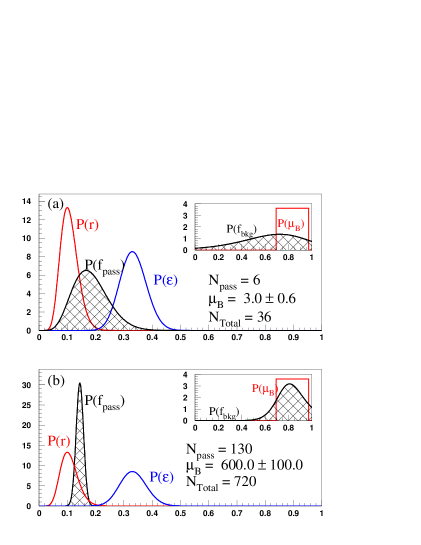
FIG. 6.: Shown are the relevant pdfs for the cross check of a possible $H^{0}\rightarrow b\overline{b}$ discovery at the CDF experiment in associated $W^{\pm}+H^{0}$ production. Plot (a) shows the fraction of the 36 events which pass the double $b$-tag requirement as a hatched histogram superimposed upon the description of the efficiency for signal $P(\varepsilon)$ and background $P(r)$. The insert of (a) shows the pdf $P(f_{bkg})$, as a hatched histogram, that best describes the observed number of events $N_{pass}$. This is to be compared with the assumed description of the background $P(\mu_{B})$. Plot (b) shows the results for a hypothetical data set twenty times the size of the Run 1 result.

The rest of Table VI shows that it is more likely to see a larger number of signal events if the efficiency of the cut on the new signal is larger, i.e. 90% instead of 30%. The last four lines of Table VI show that even if no knowledge about the efficiency of the possible new signal is claimed (except that the cut is more efficient for the signal that for the background), then the consistency $\beta$ of the initial background description to accommodate the observed 6 events is 58%, slightly higher than if the double-tag signal efficiency is described by a more precise, but overall smaller, value of $\varepsilon_{0}=$ 33%.

Tables VI illustrates some important trends in attempts to increase the confidence level of a possible signal by imposing a further cut. The most important result is that knowledge of the cut efficiency for the possible signal is useful but not necessary when trying to claim a discovery. For example, if the CDF collaboration chose to assume a uniform pdf $P(\varepsilon)$ for the efficiency of the double-tag cut on any new signal, the confidence level $\alpha_{excess}$ is still 77%. As in all measurement problems, a higher efficiency is better than a lower efficiency. This is important for increasing both the overall confidence level of the experiment $\alpha_{experiment}$ and the confidence $\beta$ that the new cut preserves the signal in a manner consistent with the original background estimate.

Example 5: Extrapolations for a Run 2 Higgs discovery

The results of Examples 3 and 4 should not discourage anyone from looking for a similar excess in a Tevatron Run 2 data set. It is trivial to scale the number of Run 1 events ($N_{Total}$) from Example 3 by the expected increase in integrated luminosity, 2 $\mbox{fb}^{-1}$ for Run 2, and solve Equation 84 for the minimum number of events $N_{pass}$ that must survive a double-tag requirement in order to have a significant excess at some arbitrary confidence level. Table VII has the results for a twenty times larger sample of events, assuming the same knowledge $P(\mu_{B})$ and $P(r)$ used in Examples 3 and 4.

TABLE VII.: Shown are the minimum number of events $N_{pass}^{disc}$ that must pass the double-tag requirement in order to claim discovery of a signal at a given confidence level $\alpha_{discovery}$, for Example 5.

$N_{Total}$	$B$	$\sigma_{B}$	$r_{pass}$	$r_{Total}$	$\alpha_{discovery}$	$N_{pass}^{disc}$
720	600	100	10	100	0.683	74
720	600	100	10	100	0.955	104
720	600	100	10	100	0.997	130

Just as was done with the real data in Example 4, it is possible to test the outcome of the Run 2 experiment with different assumptions for the efficiency of the double-tag cut on any possible signal. The results are collected in Table VIII. Figure 6b plots the results of an experiment with an assumed efficiency $\varepsilon_{0}=$ 33% for the signal where 130 events survive the double-tag cut, corresponding to a $3\sigma$ excess in the original sample.

TABLE VIII.: Shown is the confidence $\beta$ in the original description of the background $P(\mu_{B})$ assuming that $N_{pass}^{disc}$ events pass the cut with efficiency $P(\varepsilon)$.

$\alpha_{discovery}$	$N_{pass}^{disc}$	$\varepsilon_{pass}$	$\varepsilon_{Total}$	$\alpha_{experiment}$	$N_{fail}^{disc}$	$\beta$
0.683	74	33	100	0.46	31	0.81
0.955	104	33	100	0.86	28	0.51
0.997	130	33	100	0.98	25	0.23
0.683	74	90	100	0.46	31	0.97
0.955	104	90	100	0.86	28	0.88
0.997	130	90	100	0.98	25	0.76
0.683	74	uniform $P(\varepsilon)$		0.45	31	0.86
0.955	104	uniform $P(\varepsilon)$		0.81	28	0.66
0.997	130	uniform $P(\varepsilon)$		0.89	25	0.47

The insert of Figure 6b shows good agreement between $P(f_{bkg})$ and the broad $P(\mu_{B})$ used in Example 4. This implies that given the present knowledge of the efficiencies and the known processes, described by $P(\mu_{B})$, that contribute events to the $W^{\pm}+b\overline{b}$ sample, it would not be surprising to observe a $3\sigma$ excess in such a data sample from Run 2. The ultimate interpretation of such an excess should come from an improved understanding of $P(\varepsilon)$, $P(r)$ and $P(\mu_{B})$.

VIII Conclusions

The description of the measurement problem as a linear system of equations illuminates several important aspects of binomial experiments, including intuitive notions about the relative value of choosing cuts which preserve the signal of interest while rejecting non-interesting backgrounds. The use of Bayesian techniques in this solution of the binomial measurement problem offers a straightforward method of measuring signal and background fractions in both the total data sample and the subset of events which survive the application of a cut. It also provides an unbiased means of testing different cuts and is useful in evaluating potential improvements that come from increasing data samples. The method was also shown to be a powerful tool that can be used in the analysis of excess observed events over theoretical expectations.

REFERENCES

- [1] B. Noble and J. W. Daniel, Applied Linear Algebra (Prentice-Hall, 1977), p. 170.
- [2] A. Gelman, J. B. Carlin, H. S. Stern, and D. B. Rubin, Bayesian Data Analysis (Chapman & Hall, 1995) p. 31.
- [3] G. D’Agostini, Probability and Measurement Uncertainty in Physics - a Bayesian Primer, hep-ph/9512295, (1995).
- [4] D. S. Sivia, Data Analysis: A Bayesian Tutorial (Oxford University Press, 1996), p. 71.
- [5] C. Caso et al. (Particle Data Group), The European Physical Journal C3 (1998).
- [6] F. Abe et al. (CDF Collaboration), Phys. Rev. Lett. 74 2626 (1995).
- [7] S .Abachi et al. (DØ Collaboration), Phys. Rev. Lett. 74 2632 (1995).
- [8] F. Abe et al. (CDF Collaboration), Phys. Rev. D 59 092001 (1999).
- [9] F. Abe et al. (CDF Collaboration), Phys. Rev. Lett. 76 3070 (1996).
- [10] B. Abbott et al. (DØ Collaboration), submitted to Phys. Rev. D, Fermilab PUB-99/171-E, hep-ex/9906025.
- [11] B. Abbott et al. (DØ Collaboration), to be published in Phys. Rev. D, Fermilab PUB-99/015-E, hep-ex/9901040.
- [12] O. Helene, Nucl. Instrum. Methods 212. 319 (1983).
- [13] F. Abe et al. (CDF Collaboration), Phys. Rev. Lett. 79 3819 (1997).
- [14] A. Stange, W. Marciano, and S. Willenbrock, Phys. Rev. D 49 1354 (1994).