Search for ${D^{0}}\!-\!{\overline{D}\vrule width=0.0pt^{0}}$ Mixing

Abstract

We report on a search for ${D^{0}}\!-\!{\overline{D}\vrule width=0.0pt^{0}}$ mixing made by a study of the ‘wrong-sign’ process ${D^{0}}\!\to\!K^{+}\pi^{-}$. The data come from 9.0 fb^-1 of integrated luminosity of $e^{+}e^{-}$ collisions at $\sqrt{s}\approx 10\,$GeV, produced by CESR and accumulated with the CLEO II.V detector. We measure the time-integrated rate of the ‘wrong-sign’ process ${D^{0}}\!\to\!K^{+}\pi^{-}$, relative to that of the Cabibbo-favored process ${\overline{D}\vrule width=0.0pt^{0}}\!\to\!K^{+}\pi^{-}$, to be $R_{\rm ws}=(0.34\pm 0.07\pm 0.06)\%$. By a study of that rate as a function of the decay time of the ${D^{0}}$, we distinguish the rate of direct, doubly-Cabibbo-suppressed decay ${D^{0}}\!\to\!K^{+}\pi^{-}$ relative to ${\overline{D}\vrule width=0.0pt^{0}}\!\to\!K^{+}\pi^{-}$, to be $R_{D}=(0.50^{+0.11}_{-0.12}\pm 0.08)\%$. The amplitudes that describe ${D^{0}}\!-\!{\overline{D}\vrule width=0.0pt^{0}}$ mixing, $x^{\prime}$ and $y^{\prime}$, are consistent with zero. The one-dimensional limits, at the 95% C.L., that we determine are $(1/2)x^{\prime 2}<0.05\%$, and $-5.9\%<y^{\prime}<0.3\%$. All results are preliminary.

Neutral particles such as the ${K^{0}}$, ${D^{0}}$, ${B^{0}_{d}}$, and ${B^{0}_{s}}$ mesons can evolve into their respective antiparticles, the ${\overline{K}\vrule width=0.0pt^{0}}$, ${\overline{D}\vrule width=0.0pt^{0}}$, ${\overline{B}\vrule width=0.0pt^{0}_{d}}$ and ${\overline{B}\vrule width=0.0pt^{0}_{s}}\,$[1]. Measurements of the rates and mechanisms of ${K^{0}}\!-\!{\overline{K}\vrule width=0.0pt^{0}}$ and ${B^{0}_{d}}\!-\!{\overline{B}\vrule width=0.0pt^{0}_{d}}$ mixing have guided the form and content of the Standard Model, and permitted useful estimates of the masses of the charm and top quark masses, prior to direct observation of those quarks at the high energy frontier.

Within the framework of the Standard Model, the rate of ${D^{0}}\!-\!{\overline{D}\vrule width=0.0pt^{0}}$ mixing is expected to be small, for two reasons. First, the decays of the ${D^{0}}$ are Cabibbo favored, while the mixing amplitudes are doubly-Cabibbo-suppressed, and second, the GIM cancellation[2] is thought to cause substantial additional suppression. Many interesting extensions to the Standard Model predict enhancements to the rate of ${D^{0}}\!-\!{\overline{D}\vrule width=0.0pt^{0}}$ mixing[3], much as the charm and top quarks enhance the rates of ${K^{0}}\!-\!{\overline{K}\vrule width=0.0pt^{0}}$ and ${B^{0}_{d}}\!-\!{\overline{B}\vrule width=0.0pt^{0}_{d}}$ mixing.

We report here on a study of the process, ${D^{0}}\!\to\!K^{+}\pi^{-}$ (those processes obtained by the application of charge conjugation on all particles, such as, in this case, ${\overline{D}\vrule width=0.0pt^{0}}\!\to\!K^{-}\pi^{+}$, are implied throughout this report). We use the charge of the ‘slow’ pion, $\pi_{s}^{+}$, from the decay $D^{*+}\!\to\!{D^{0}}\pi^{+}_{s}$ to deduce production of the ${D^{0}}$, and then we seek the rare, ‘wrong-sign’ $K^{+}\pi^{-}$ final state, in addition to the more frequent ‘right-sign’ final state, $K^{-}\pi^{+}$.

The wrong-sign process, ${D^{0}}\!\to\!K^{+}\pi^{-}$, can proceed either through direct, doubly-Cabibbo-suppressed decay (DCSD) via the Feynman diagram portrayed in Fig. 1, or through mixing followed by the Cabibbo-favored decay (CFD), ${D^{0}}\!\to\!{\overline{D}\vrule width=0.0pt^{0}}\!\to\!K^{+}\pi^{-}$. Both processes contribute to the ‘wrong-sign’ rate, $R_{\rm ws}$:

$$R_{\rm ws}=\displaystyle{\Gamma({D^{0}}\!\to\!K^{+}\pi^{-})\over\Gamma({\overline{D}\vrule width=0.0pt^{0}}\!\to\!K^{+}\pi^{-})}.$$

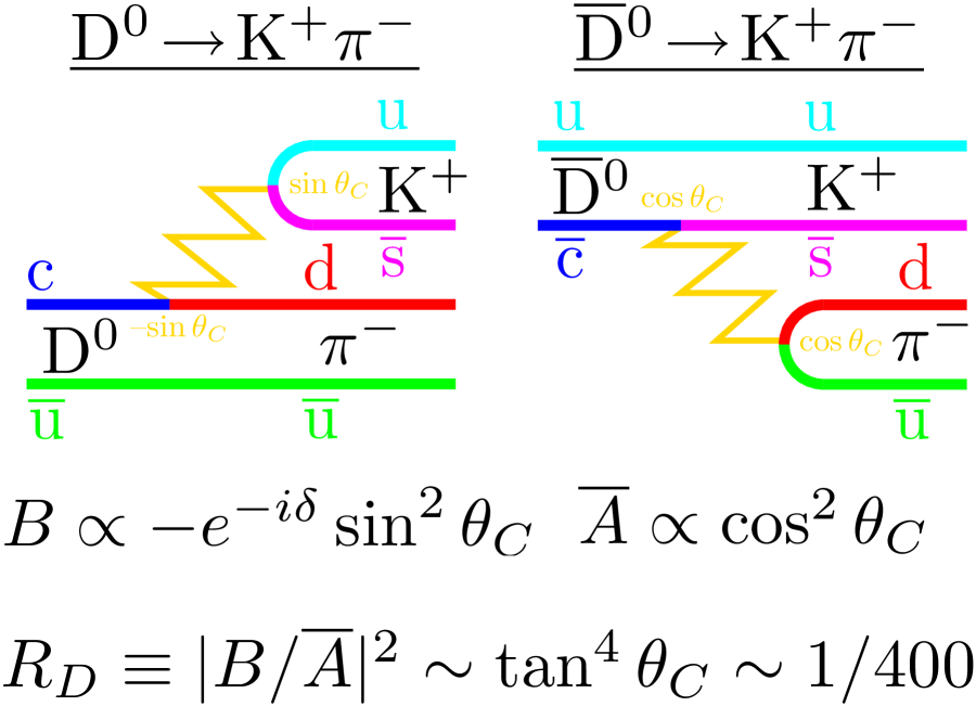
FIG. 1.: The Feynman diagrams for the decays ${D^{0}}\!\to\!K\pi$. The ‘wrong-sign’ decay, with amplitude denoted $B$, is shown on the left, and the ‘right-sign’ decay, with amplitude denoted $\overline{A}$, is shown on the right. The Cabibbo angle is $\theta_{C}$, and $\delta$ is a possible relative strong phase between the processes shown. The ratio of decay rates is denoted $R_{D}$ and is expected to be of order $\tan^{4}\theta_{C}\!\sim\!1/400\!=\!0.25\%$.

To disentangle the two processes that could contribute to ${D^{0}}\!\to\!K^{+}\pi^{-}$, we study the distribution of wrong-sign final states as a function of the proper decay time, $t$, of the ${D^{0}}$. The mixing amplitude grows, relative to the decay amplitude, by a factor of $-(1/2)(ix+y)t$, as portrayed in Fig. 2. We refer to the proper decay time $t$ in units of the mean ${D^{0}}$ lifetime, $\tau_{{D^{0}}}=415\pm 4\,$fs[4]. Then, we refer to the mixing amplitude for ${D^{0}}\!\to\!{\overline{D}\vrule width=0.0pt^{0}}$, in appropriate units: those of one-half the mean ${D^{0}}$ decay rate, $\Gamma_{{D^{0}}}/2=1/[2\tau_{{D^{0}}}]$. The mixing amplitude through virtual intermediate states is $x$, and that through real intermediate states by $y$[5]. When conservation of $CP$ is assumed:

$$\begin{array}[]{rcccl}x&=&\displaystyle{\Delta M\over\Gamma_{{D^{0}}}}&=&\displaystyle{M_{12}\over\Gamma_{{D^{0}}}/2\vspace{2mm}}\\ y&=&\displaystyle{\Delta\Gamma\over 2\Gamma_{{D^{0}}}}&=&\displaystyle{\Gamma_{12}/2\over\Gamma_{{D^{0}}}/2}\end{array}.$$

We use the convention that $y\!>\!0(y\!<\!0)$ corresponds to a shorter(longer) than average lifetime for eigenstates of $CP$ with the same eigenvalue as the $\pi^{+}\pi^{-}$ state populated by ${D^{0}}\!\to\!\pi^{+}\pi^{-}$.

It is likely, although not inevitable, that $|x|\!\sim\!|y|$ within the Standard Model[6]. Extensions to the Standard Model contribute to $x$ alone.

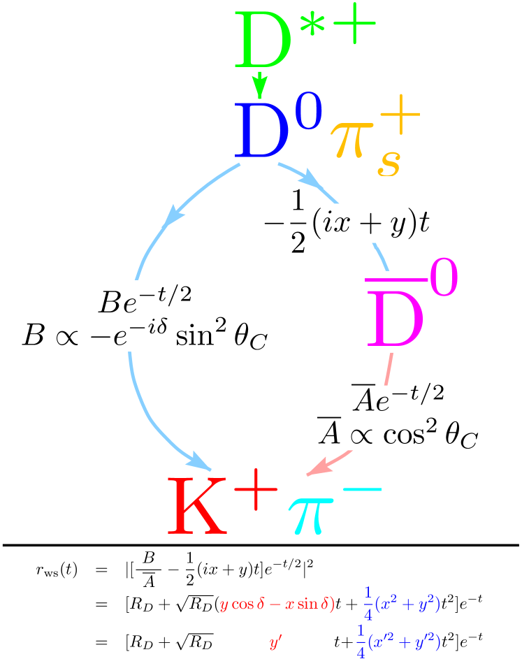
FIG. 2.: The two processes that yield wrong-sign $K\pi$. The proper decay time of the ${D^{0}}$, in units of the mean ${D^{0}}$ lifetime, is denoted $t$. The strong decay of the $D^{*+}\!\to\!{D^{0}}\pi_{s}^{+}$ specifies $t=0$, and the charge of the slow pion $\pi_{s}^{+}$ distinguishes a ${D^{0}}$ from a ${\overline{D}\vrule width=0.0pt^{0}}$. The ${D^{0}}$ can undergo direct, doubly-Cabibbo-suppressed decay (DCSD), to $K^{+}\pi^{-}$, schematically represented by the route to the left, with amplitude $Be^{-t/2}$. The ${D^{0}}$ might also mix, with amplitude $-(1/2)(ix+y)t$, schematically represented by the route to the right, into a ${\overline{D}\vrule width=0.0pt^{0}}$, and then undergo Cabibbo-favored decay (CFD) into $K^{+}\pi^{-}$. The interference of these two amplitudes gives the relative decay rate to $K^{+}\pi^{-}$ as a function of $t$, $r_{\rm ws}(t)$, shown. The quantity $y^{\prime}$ is defined to be $y\cos\delta-x\sin\delta$, and $x^{\prime}$ is defined analogously, $x^{\prime}=x\cos\delta+y\sin\delta$.

The possible interference between direct decay and mixing would cause the number of wrong-sign decays, relative to the total number of right-sign decays, as a function of $t$, $r_{\rm ws}(t)$ to be[10, 11]

$$r_{\rm ws}(t)=[R_{D}+\sqrt{R_{D}}y^{\prime}t+\displaystyle{1\over 4}(x^{\prime 2}+y^{\prime 2})t^{2}]e^{-t},$$ (1)

where $R_{D}$ is the ratio of wrong-sign to right-sign rates of direct decay. The ${D^{0}}\!-\!{\overline{D}\vrule width=0.0pt^{0}}$ mixing amplitudes $x^{\prime}$ and $y^{\prime}$ are defined by:

$$\begin{array}[]{rcl}y^{\prime}&\equiv&y\cos\delta\!-\!x\sin\delta\\ x^{\prime}&\equiv&x\cos\delta\!+\!y\sin\delta\end{array},$$

where $\delta$ is a possible strong phase between the wrong-sign and right-sign decay amplitudes. In a sense, use of a hadronic final state, such as $K\pi$, ‘filters’ the mixing amplitudes, much as a polarizer filters light. There are plausible arguments that $y^{\prime}>0$[7], and $\delta<13^{\circ}$[8, 9].

We report here on the analysis of data accumulated between 1995 and 1999 from an integrated luminosity of $9.0\,$fb^-1 of $e^{+}e^{-}$ collisions with $\sqrt{s}\approx 10\,$GeV at the Cornell Electron Storage Rings (CESR). The data were taken with CLEO II multipurpose detector [12], which includes two cylindrical drift chambers in a superconducting solenoid ($B=1.5\,$T) for measurement of the three-momentum $\vec{p}$ of charged particles, a cylindrical array of CsI crystals for measurement of the energies of photons and electrons, and a system of iron absorbers interleaved with proportional chambers for the identification of muons. These systems cover approximately 80% of the solid angle around the $e^{+}e^{-}$ annihilation point.

In 1995 a silicon vertex detector (SVX) was installed [13], that enables both precise reconstruction of the proper lifetime of short-lived particles such as the ${D^{0}}$, as well as improved reconstruction of the angle $\theta$ between the $e^{+}e^{-}$ beams and the momentum vector of low-momentum charged particles, such as the slow charged pion from the decay $D^{*+}\!\to\!{D^{0}}\pi_{s}^{+}$. Also, in 1995, the gas in the larger CLEO II drift chamber was changed from argon-ethane to a helium-propane mixture, resulting in improved momentum and mass resolution, and improved particle identification by specific ionization $(dE/dx)$. We refer to this revised configuration of the CLEO II detector as CLEO II.V.

We reconstruct candidates for the decay sequences $D^{*+}\!\to\!\pi^{+}_{s}{D^{0}}$, followed by either ${D^{0}}\!\to\!K^{+}\pi^{-}$ (wrong-sign, or WS) or ${D^{0}}\!\to\!K^{-}\pi^{+}$ (right-sign, or RS). The sign of the slow charged pion, either $\pi^{+}_{s}$ or $\pi^{-}_{s}$, identifies (‘tags’) the charm state at production (‘$t=0$’) as either ${D^{0}}$ or ${\overline{D}\vrule width=0.0pt^{0}}$. The broad features of the reconstruction are similar to those employed in the recent CLEO measurement of the $D$ meson lifetimes [14], but there are four principal differences. First, we accept candidates with total momentum, $p_{D^{*}}$, as low as $2.2\,$GeV; we show the approximate $D^{*}$ production cross section as a function of $p_{D^{*}}$ in Fig. 3. Second, we fully exploit the three-dimensional tracking capability of the SVX. We reject candidates where the daughter tracks form poor vertices in three-dimensional space, and we sharpen the reconstructed direction of the $\pi^{+}_{s}$ momentum, thereby improving our resolution for reconstruction of $Q$, the (small) energy released in the $D^{*+}\!\to\!\pi^{+}_{s}{D^{0}}$ decay. We denote by $M$ the reconstructed mass of the two daughters of the ${D^{0}}$, and by $M_{K\pi\pi}$ the reconstructed mass of all three particles in the candidate. We reconstruct $Q=(M_{K\pi\pi}-M-m_{\pi})c^{2}$, where $m_{\pi}$ is the mass of a charged pion. Third, we require candidates to be well-measured in $Q$, and in $M$. Fourth, we require candidates to pass two ‘kinematic’ requirements, designed to suppress backgrounds from ${D^{0}}\!\to\!\pi^{+}\pi^{-}$, ${D^{0}}\!\to\!K^{+}K^{-}$, ${D^{0}}\!\to\,>\!2\,$bodies, and from cross-feed between WS and RS. For the first kinematic requirement, for ${D^{0}}\!\to K^{+}\pi^{-}$ candidates we evaluate the mass $M$ under the three alternate hypotheses ${D^{0}}\!\to\!\pi^{+}\pi^{-}$, ${D^{0}}\!\to\!K^{+}K^{-}$, and ${D^{0}}\!\to\!\pi^{+}K^{-}$. If any one of the three masses so computed falls within $30\,$MeV/c² (approximately $4.5\,\sigma$) of the ${D^{0}}$ mass, the ${D^{0}}\!\to K^{+}\pi^{-}$ candidate is rejected. A conjugate requirement is made for the RS decays. The second kinematic requirement rejects one of the two configurations of very asymmetric decay, with a requirement that the decay angle $\theta^{*}$ of the hypothesized kaon, $\theta^{*}$, in the ${D^{0}}$ rest frame, with respect to the ${D^{0}}$ boost, satisfy $\cos\theta^{*}<0.8$. This requirement removes candidates with slow pions from the ${D^{0}}$ decay.

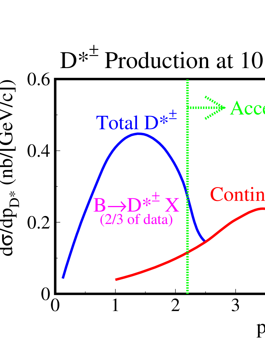
FIG. 3.: The $D^{*\pm}$ production cross section at $\sqrt{s}=10.58\,$GeV[4, 15]. The $D^{*\pm}$ at higher momenta result from the continuum production: $e^{+}e^{-}\!\to\!c\overline{c}$, followed by hadronization of charmed quarks to a $D^{*\pm}$, and these $D^{*\pm}$ are present for all of our data. The component of $D^{*\pm}$ at lower momenta are present in the 2/3 of the data taken with $\sqrt{s}$ at the mass of the $\Upsilon(4s)$, and these softer $D^{*\pm}$ result from the decay $B\!\to\!D^{*\pm}X$. We accept $D^{*\pm}$ with momenta greater than $2.2\,$GeV/$c$; most of these are from continuum production.

The CLEO drift chamber system allows reconstruction of the specific ionization ($dE/dx$) deposited by the passage of charged particles, permitting an independent assessment of the identification of a charged particle as either a $\pi$ or a $K$. We require that the $dE/dx$ be within three standard deviations ($\sigma$) of the hypothesis used in the reconstruction of $M$ and $Q$; this is a loose, consistency requirement. We tighten $dE/dx$ criteria only for the evaluation of systematic errors.

A total of $16126\pm 127$ candidates for the right-sign decay pass all requirements; their distribution in $Q$ and $M$ is shown in Fig. 4.

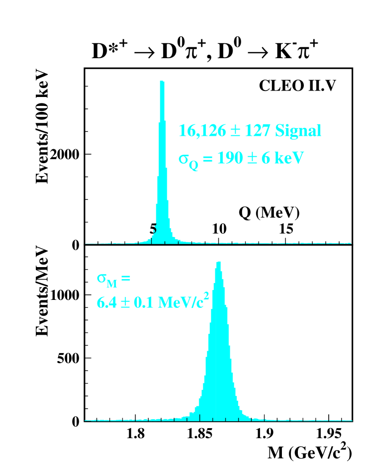
FIG. 4.: Signal for the right-sign process ${D^{0}}\!\to\!K^{-}\pi^{+}$. The events in the top and bottom plots come from the same sample, and are all candidates for the decay $D^{*+}\!\to\!\pi^{+}_{s}{D^{0}}$ followed by ${D^{0}}\!\to\!K^{-}\pi^{+}$. In the top plot, the horizontal axis is $Q$, the energy released in the decay of the $D^{*+}$, for events where the reconstructed mass $M$ of the $K\pi$ system falls within 15 MeV/c² of the ${D^{0}}$ mass. In the bottom plot, the horizontal axis is $M$, for events where $Q$ falls within 450 keV/c² of its nominal value. The total number of right-sign signal events is $16126\pm 127$. The experimental resolution function in $Q$ is non-gaussian, due to a substantial dependence of the width of the specific (gaussian) resolution on the particular decay configuration; the $\sigma_{Q}$ shown is the core value from a fit to a bifurcated Student’s $t$ distribution. The result for $\sigma_{M}$ comes from a fit to a double gaussian.

The population of the wrong-sign candidates is shown on a scatter plot of $Q$ versus $M$ in Fig. 5. In Fig. 5, several prominent background features are evident. The combination of ${\overline{D}\vrule width=0.0pt^{0}}\!\to\!K^{+}\pi^{-}$ with random slow pions, $\pi^{+}$, causes the vertical ‘ridge,’ with $M$ equal to the mass of the ${D^{0}}$, $M_{{D^{0}}}$. The phenomenon is sometimes called ‘dilution’, and we will refer to it as ‘random $\pi^{\pm}+{D^{0}}/{\overline{D}\vrule width=0.0pt^{0}}$’. A diffuse background is also evident, due to the random combination of charged particles from $e^{+}e^{-}\!\to$light quarks, and from $e^{+}e^{-}\!\to\!c\overline{c}$, which we will refer to as combinatoric ‘$uds$’ and ‘$c\overline{c}$,’ respectively. There is also a broad enhancement near the signal in $Q$, but at $M<M_{{D^{0}}}$, due to processes such as ${D^{0}}\!\to\!K^{-}\rho^{+}$, followed by a very asymmetric decay $\rho^{+}\!\to\!\pi^{0}\pi^{+}$, resulting in a $\pi^{0}$ that is nearly at rest. Since a number of modes that we model can produce such behavior, including ${D^{0}}\!\to\!\rho^{+}\pi^{-}$, ${D^{0}}\!\to\!\rho^{-}\pi^{+}$, and ${D^{0}}\!\to\!K^{*-}\pi^{+}$, we refer to this type of background as ‘PV’, for pseudoscalar-vector.

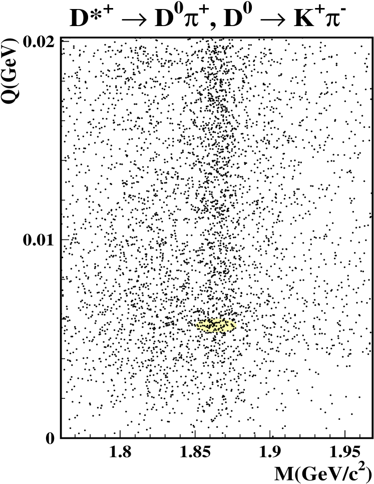
FIG. 5.: Scatter plot of $Q$ versus $M$ for the candidates for ${D^{0}}\!\to\!K^{+}\pi^{-}$. The signal region is lightly shaded. The most prominent feature is the vertical ‘ridge’ at $M_{{D^{0}}}$ ; this results from the combination of the CFD ${\overline{D}\vrule width=0.0pt^{0}}\!\to\!K^{+}\pi^{-}$ with a random slow pion $\pi^{+}$, which combine to fake a $D^{*+}$. The pervasive, smooth background consists of random combinations of charged tracks, referred to as $c\overline{c}$ and $uds$ background in the text. The background density for $M\!<\!M_{{D^{0}}}$ exceeds that for $M\!>\!M_{{D^{0}}}$ simply due to phase space for the random combinations, and also due to true ${D^{0}}$ decays where a particle has been missed, resulting in a reduction in $M$. The so-called ‘PV’ background, described in the text, causes an increase in density near the signal in $Q$, but at $M<M_{{D^{0}}}$.

To deduce the wrong-sign rate, $R_{\rm ws}$, we perform a 2-dimensional fit to the region of the $Q$ versus $M$ plane shown in Fig. 5. Each of the background shapes: ‘random $\pi^{\pm}+{D^{0}}/{\overline{D}\vrule width=0.0pt^{0}}$’, $c\overline{c}$, $uds$, and PV is taken from Monte Carlo simulated data, which statistics corresponding to 90 fb^-1 of integrated luminosity, but the normalization of each component is allowed to float in the fit; only the $uds$ shows a significant difference with its expected contribution; the fit exceeds expectation by approximately a factor of two. The wrong-sign signal shape is taken directly from a seven $\sigma$ ellipse around the right-sign signal. The fitted background composition, superposed on the data, and projected on to $Q$ and $M$ are shown in Fig. 6. The event yields in the signal region from the fit are summarized in Table I.

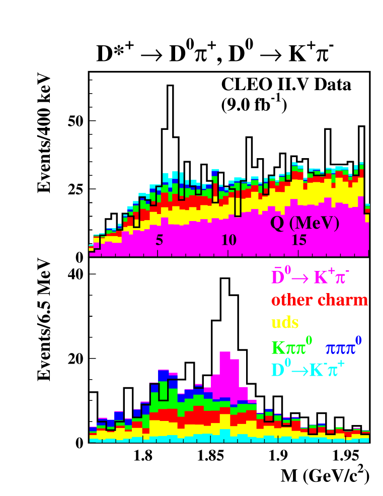
FIG. 6.: Signal for the wrong-sign process ${D^{0}}\!\to\!K^{+}\pi^{-}$. See also the caption for the right-sign analog, Fig. 4. The solid lines are the data, and the colored regions are the contributions from various background sources from the fit, as labeled, with shapes from simulation, and levels from a fit to the two-dimensional plane of $Q$ and $M$. The fit to the signal peak is not shown. The results of the fit are summarized in Table I.

No acceptance corrections are need to directly compute, from Table I, $R_{\rm ws}=(0.34\pm 0.07)\%$. The dominant systematic errors all stem from the potentially inaccurate modeling of the initial and acceptance-corrected shapes of the background contributions in the $Q$-$M$ plane. We assess these systematic errors by substantial variation of the fit regions, $dE/dx$ criteria, and kinematic criteria; the total systematic error we assess is $0.06\%$.

Our complete result for $R_{\rm ws}$ is summarized in Table II.

There are two directly comparable measurements of $R_{\rm ws}$: one is from CLEO II[16], $R_{\rm ws}=(0.77\pm 0.25\pm 0.25)\%$ which used a data set independent of that used here; the second is from Aleph[17], $R_{\rm ws}=(1.84\pm 0.59\pm 0.34)\%$; comparison of our result and these are marginally consistent with $\chi^{2}=6.0$ for 2 DoF, for a C.L. of 5.0%.

TABLE II. Result for $R_{\rm ws}$. For the branching ratio ${\cal B}({D^{0}}\!\to\!K^{+}\pi^{-})$, we take the absolute branching ratio ${\cal B}({\overline{D}\vrule width=0.0pt^{0}}\!\to\!K^{+}\pi^{-})=(3.85\pm 0.09)\%$, and the third error results from the uncertainty in this absolute branching ratio.

Quantity	Result
$R_{\rm ws}$	$(0.34\pm 0.07\pm 0.06)\%$
$R_{\rm ws}/\tan^{4}\theta_{C}$	$(1.28\pm 0.25\pm 0.21)$
${\cal B}({D^{0}}\!\to\!K^{+}\pi^{-})$	$(1.31\pm 0.26\pm 0.22\pm 0.03)\!\times\!10^{-4}$

We have split our sample into candidates for ${D^{0}}\!\to\!K^{+}\pi^{-}$ and ${\overline{D}\vrule width=0.0pt^{0}}\!\to\!K^{-}\pi^{+}$. There is no evidence for a $CP$-violating time-integrated asymmetry. From Table II, it is straightforward to evaluate the $1\sigma$ statistical error on the $CP$ violating time-integrated asymmetry as $\sqrt{107}/54.8=19\%$.

Given the absence of a significant time-integrated $CP$ asymmetry, we undertake a study of the decay time dependence of the wrong-sign rate in which $CP$ conservation is assumed. Our fits use Equation 1, which describes the wrong-sign decay time dependence, include the term that is linear in $t$, unless specifically noted. The fit variable $y^{\prime}$ is allowed to vary over all real values, and we thereby account for the principal objection[18] to an earlier analysis of ${D^{0}}\!-\!{\overline{D}\vrule width=0.0pt^{0}}$ mixing[19]. We believe that the fact that our acceptance in $t$ extends all the way to zero lifetimes, while the acceptance for the fixed target experiments E691 and E791[19, 18] dropped near $t\!\sim\!1/2$, prevents the loss in sensitivity that E791[18] reported.

We reconstruct $t$ using only the vertical, or $y$, component of the flight distance of the ${D^{0}}$. This reconstruction is guided by the physical dimensions of the CESR luminous region[20] and is portrayed in Fig. 7. We reconstruct the ${D^{0}}$ decay point, $(x_{v},y_{v},z_{v})$, with a resolution that is typically $40\,\mu$m in each dimension. We measure the centroid of the luminous region, $(x_{b},y_{b},z_{b})$ with suitable hadronic events in blocks of data that typically contain integrated luminosities of several pb^-1. Runs where $y_{b}$ is poorly measured are discarded, and the dominant error on $y_{v}-y_{b}$ comes from $y_{v}$. We reconstruct $t$ as:

$$t=\displaystyle{M\over p_{y}}\times\displaystyle{y_{v}-y_{b}\over c\tau_{{D^{0}}}}$$

where $p_{y}$ is the $y$-component of the total momentum of the $K^{+}\pi^{-}$ system. The error $\sigma_{t}$ is typically $1/2$, although when the ${D^{0}}$ direction is near the horizontal, $\sigma_{t}$ can be large; we reject candidates with $\sigma_{t}>3/2$.

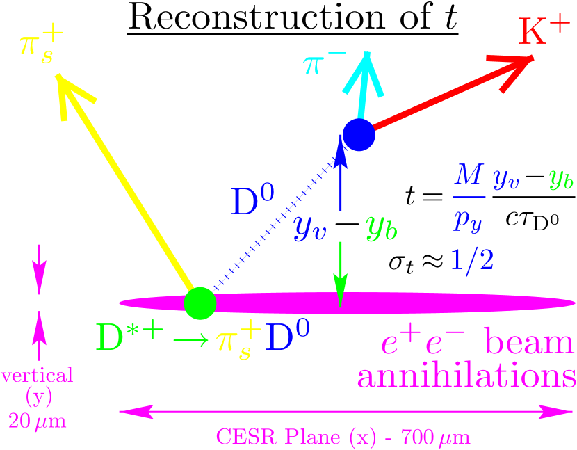
FIG. 7.: The reconstruction of $t$. We measure the proper decay time of the ${D^{0}}$, $t$, in multiples of the mean ${D^{0}}$ lifetime, or $t=\tau/\tau_{{D^{0}}}$, where $\tau$ is the proper decay time measured in seconds. As shown in this diagram, the region of $e^{+}e^{-}$ annihilation is very small in the vertical, or $y$, where the region extends only $20\,\mu$m at FWHM. In the bend plane of the CESR collider, or $x$, the FWHM extends $700\,\mu$m, and along the beam axis or $z$, the FWHM is $30,000\,\mu$m. The typical three-dimensional flight distance of the ${D^{0}}$ is $180\,\mu$m, which is small compared to the $x$ and $z$ extents of the luminous region. We therefore reconstruct $t$ using the displacement of the ${D^{0}}$ decay point, or vertex, in $y$ from the beam centroid using the formula as shown. The symbol $y_{v}$ refers to the $K^{+}\pi^{-}$ vertex, and $y_{b}$ refers to the beam centroid. The typical resolution in $t$ is $\sigma_{t}\approx 1/2$, and $\sigma_{t}$ becomes large when the direction of the ${D^{0}}$ flight is near to the horizontal. The error in extrapolation of the $\pi^{+}_{s}$ back to the luminous region is large, due to multiple scattering in the beam pipe, and indeed, reconstruction of the $\pi^{+}_{s}$ direction benefits greatly by constraint of the $\pi_{s}^{+}$ to the intersection of the beam and the extrapolated ${D^{0}}$ flight path. Use of other tracks in the event typically do not improve reconstruction of the estimate of the $D^{*+}$ production point beyond that shown.

In the sample of right-sign, ${\overline{D}\vrule width=0.0pt^{0}}\!\to\!K^{+}\pi^{-}$ decays, $14199\pm 120$ signal events pass the requirements for the reconstruction of $t$, out of the initial sample of $16126\pm 126$ used for the measurement of $R_{\rm ws}$. The distribution in $t$ of the right-sign events is shown in Fig. 8. We fit that distribution in the manner described in our measurement of mean charm lifetimes[14], and find, in units of the recent world average[4] mean ${D^{0}}$ life, $0.972\pm 0.014$, where no systematic error for this measurement is assessed. Since we have not assessed a systematic error, this result should not be construed as a new result on $\tau_{{D^{0}}}$. However, possible systematic errors due to the reconstruction and fitting technique are limited by this result from the right-sign data. There are far fewer events in the wrong-sign data, and so this class of systematic errors is negligible compared to the statistical error of the fit to the wrong-sign data.

The fit to the right-sign data determines the resolution function that we use for the fit of the wrong-sign data. We also use the mean ${D^{0}}$ lifetime from the fit to the right-sign data as the central value for various charm backgrounds that are present in the wrong-sign data.

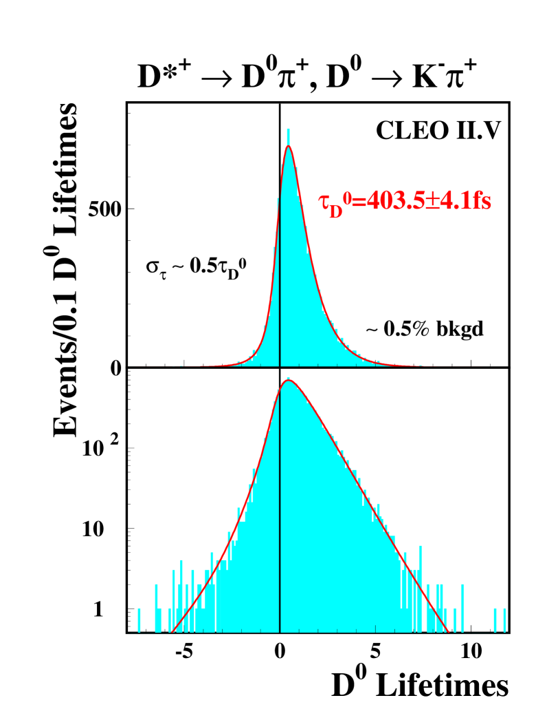
FIG. 8.: Distribution in $t$ for right-sign ${D^{0}}\!\to\!K^{-}\pi^{+}$. The histogram shows the data, and those data are the same for the upper and lower plots; the only difference is the vertical scale, linear above, logarithmic below. The smooth curve is the fit, which results in the mean life shown of $\tau_{{D^{0}}}=403.5\pm 4.1\,$fs, where the error is statistical alone. We have not assessed the systematic error on the fit to $\tau_{{D^{0}}}$, so, it should not be construed as a new result on $\tau_{{D^{0}}}$.

Our resolution function is displayed, as well as the effect of folding that function with each of the three functional forms, $e^{-t}$, $te^{-t}$, and $t^{2}e^{-t}$, that enter in the time-dependent rate of wrong-sign decays from Equation 1, in Fig. 9. For the forms $te^{-t}$ and $t^{2}e^{-t}$, the breadth of the distribution is dominantly from the functional forms themselves; a narrowing of the resolution function would not greatly help distinguish between them.

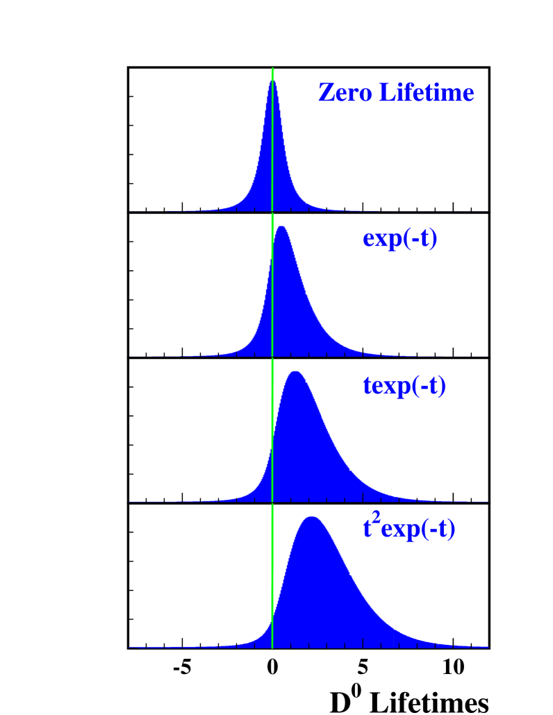
FIG. 9.: The functional forms of decay and mixing, as a function of the proper time $t$, relative to the mean ${D^{0}}$ lifetime. The top plot shows our resolution function, as determined from the fit in Fig. 8, which can be approximately characterized by a gaussian with resolution $\sigma_{t}\!\approx\!1/2$. The subsequent three plots show this resolution function convolved with the three functional forms evident in Eq. 1: $e^{-t}$, $te^{-t}$, and $t^{2}e^{-t}$, which describe, respectively, DCSD decay, interference between DCSD decay and mixing, and mixing.

In the sample of wrong-sign, ${D^{0}}\!\to\!K^{+}\pi^{-}$ decays, 91 events pass the requirements for the reconstruction of $t$, out of the initial sample of 107 events in the signal region described in Table I, and used for the measurement of $R_{\rm ws}$. The distribution in $t$ of the 91 wrong-sign events is shown in Fig. 10. We fit that distribution in the manner distinct from that used in our measurement of mean charm lifetimes[14].

We estimate the composition of the 91 events by applying the same requirement to the (renormalized) Monte Carlo sample used to fit for $R_{\rm ws}$. A summary of the composition appears in Table III.

We fit the distribution of wrong-sign candidates displayed in Fig. 10 with a superposition of $r_{\rm ws}(t)$, from Equation 1; an exponential with the ${D^{0}}$ lifetime for the ‘$\pi^{\pm}+{D^{0}}/{\overline{D}\vrule width=0.0pt^{0}}$’ background; a zero-lifetime component for the $uds$ background; and second exponential to describe the $c\overline{c}$ and PV backgrounds. All distributions in $t$ are folded with our resolution function. A Poisson likelihood, based on the extended maximum likelihood technique[21], is computed, for bins that are $1/10$ of a ${D^{0}}$ lifetime, which is much smaller than $\sigma_{t}$.

The mean lifetime of the Monte Carlo simulated data, after renormalization for the fit to the $Q\!-\!M$ plane, agrees very well with the data, outside of the signal region. This agreement gives us confidence in the use of the Monte Carlo simulated data to describe the background in the signal region. In the Monte Carlo simulated data, the decay time distribution of the $c\overline{c}$ and PV backgrounds is well described with a single exponential, folded with the resolution function. We use the mean ${D^{0}}$ lifetime to describe that exponential, but we explicitly vary that lifetime by $\pm 15\%$ to assess a systematic error.

The information on the expected fractions of the various background components, as it appears in Table III, is incorporated as a a separate constraint added to the likelihood. The error on each fraction is nominally $(\sigma^{2}_{P}+\sigma^{2}_{F})^{1/2}$, except for the signal component, where $\sigma_{F}$ is omitted. The systematic errors, $\sigma_{S}$ from Table III, are included when the systematic errors on the fit parameters are evaluated.

TABLE III. Event yields in the $Q-M$ signal region for wrong-sign ${D^{0}}\!\to\!K^{+}\pi^{-}$ candidates that have had $t$ successfully reconstructed. The distribution in $t$ itself is shown in Fig. 10. The event yields in the second column are taken from the same fit to the data described in Table I, but with the effects of successful $t$ reconstruction taken into account by the study of our sample Monte Carlo simulated data, which corresponds to an integrated luminosity of 90 fb^-1. The statistical errors on the number of events, in the second column, result from the fit to the whole $Q\!-\!M$ plane; since the signal populates the signal region with high efficiency, the errors on the ${D^{0}}\!\to\!K^{+}\pi^{-}$ signal are the full Poisson errors on the mean yield of events. The statistical errors on the background components from the fit are relatively small compared to the Poisson error that corresponds to the mean event yield; a far greater number of background events populate the entire $Q\!-\!M$ plane than populate the signal region alone. The third column gives the fraction of the wrong-sign (WS) sample constituted by the signal and each category of background; the fourth column gives the Poisson error $\sigma_{P}$, corresponding to any one random sample drawn from a distribution with the mean yield of events, on that fraction. The fifth and sixth columns give the error $\sigma_{F}$ on each fraction from the fit to the whole $Q\!-\!M$ plane, and then the error $\sigma_{S}$ from systematic effects, determined principally from varying fit regions in the $Q\!-\!M$ plane. For combining errors, $\sigma_{P}$ and $\sigma_{F}$ are counted only once for the signal. The last column shows the mean life of the background components, with our estimated systematic error on that mean life, in units of the mean ${D^{0}}$ lifetime. For the signal ${D^{0}}\!\to\!K^{+}\pi^{-}$, the mean life is unknown (unk.) and can vary, according to Eqn. 1, between 0.586 and 3.414. For reference, the right-sign yield and measured mean life with error is given in the last row.

	#	%	%	%	%
Component	Events	WS	$\mathbf{\sigma_{P}}$	$\mathbf{\sigma_{F}}$	$\mathbf{\sigma_{S}}$	$\langle t\rangle$
WS Data	$91$	100
${D^{0}}\!\to\!K^{+}\pi^{-}$	$49.7\pm 9.8$	54.6	10.8	10.8	8.7	unk., .59-3.4
Backgrounds:
$\pi^{\pm}+{D^{0}}/{\overline{D}\vrule width=0.0pt^{0}}$	$19.6\pm 1.4$	21.5	4.9	1.5	2.5	$.972\pm 0.014$
$c\overline{c}$	$10.4\pm 1.1$	11.4	3.5	1.2	1.4	$1.00\pm 0.28$
$uds$	$5.1\pm 0.6$	5.6	2.5	0.7	1.2	$.004\pm 0.015$
PV	$6.2\pm 0.7$	6.8	2.7	0.8	0.8	$1.17\pm 0.25$
${D^{0}}\!\to\!K^{-}\pi^{+}$	$14199$					$.972\pm 0.014$

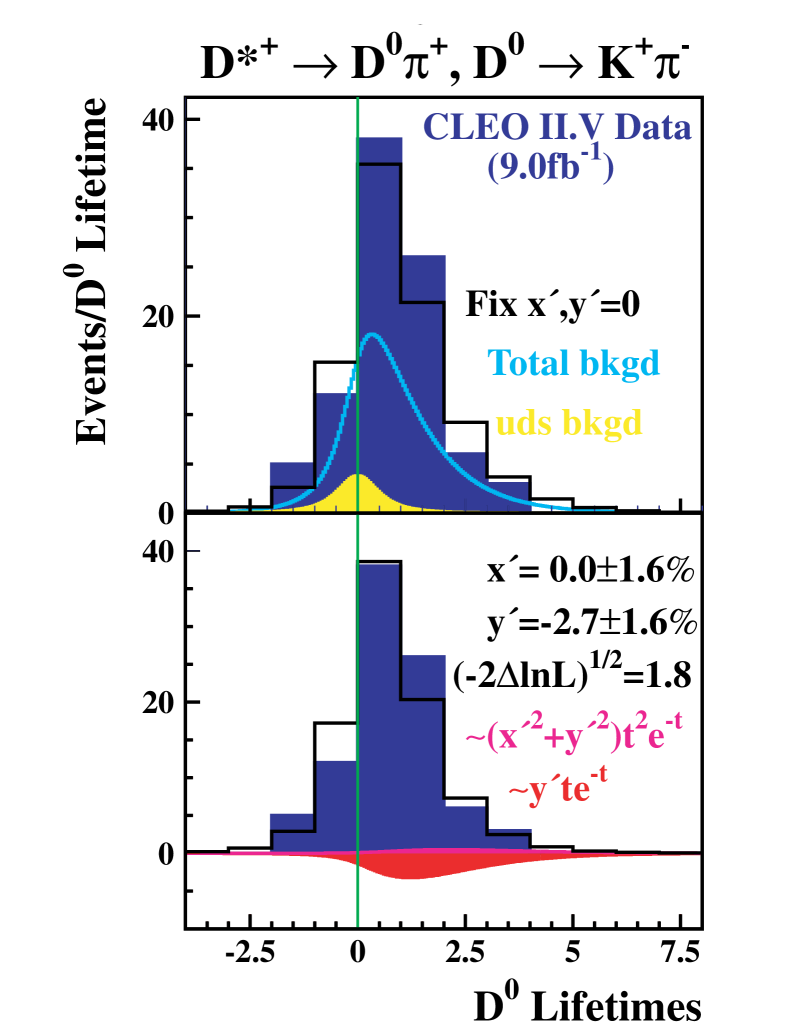
FIG. 10.: Distribution in $t$ for wrong-sign ${D^{0}}\!\to\!K^{+}\pi^{-}$. The same histogram of data is shown in both the upper and lower plots; the differences are the fit results shown and overlayed. The solid black lines are the totals of all components of the fits. The values of $x^{\prime}$ and $y^{\prime}$, from Eqn. 1, are fixed to zero in the fit displayed in the upper plot. The best-fit shapes from total and $uds$ backgrounds are shown as smooth curves. The variables $x^{\prime}$ and $y^{\prime}$ float freely in the lower fit, and the best-fit values are shown. The likelihood decrement from the upper to lower fit gives $\sqrt{-2\Delta\ln{\cal L}}=1.8\,\sigma$. The best-fit shapes of the two mixing terms are shown, although only that from $te^{-t}$ is visible.

Six parameters are able to vary in the fit: $x^{\prime}$, $y^{\prime}$, $a_{D}$ where $R_{D}=a_{D}^{2}$, all from Equation 1; and the fraction of each of the $\pi^{\pm}+{D^{0}}/{\overline{D}\vrule width=0.0pt^{0}}$, combined $c\overline{c}+$PV, and $uds$ backgrounds.

The fit has been tested on 73 samples synthesized from the right-sign candidates, and background from the sidebands in the wrong-sign $Q\!-\!M$ plane. Each of the synthesized samples contains 91 events, and they are composed to represent the wrong-sign sample described in Table III. The fits to the 73 synthetic samples show no bias in fitted values of $x^{\prime}$, $y^{\prime}$, and $a_{D}$. They also verify the ability of the fit to estimate our statistical errors.

In the initial fit to the actual wrong-sign data, $x^{\prime}$ and $y^{\prime}$ are constrained to be zero, and this fit is shown in the upper part of Fig. 10; the confidence level of that fit is $84\%$, indicating a good fit.

The mixing amplitudes $x^{\prime}$ and $y^{\prime}$ are then allowed to freely vary, and the best fit values are shown in both the lower portion of Fig. 10, and in Table IV.

TABLE IV. Results of the fit to the distribution of ${D^{0}}\!\to\!K^{+}\pi^{-}$ in $t$. Both the distribution, and the fit, are shown in the lower portion of Fig. 10.

Parameter	Best Fit	95% C.L.
$A^{A^{A}}$$R_{D}$	$(0.52^{+0.11}_{-0.12}\pm 0.08)\%$
$y^{\prime}$	$(-2.7^{+1.5}_{-1.6}\pm 0.2)\%$	$-5.9\%<y^{\prime}<0.3\%$
$x^{\prime}$	$(0\pm 1.6\pm 0.2)\%$	$|x|<3.2\%$
$(1/2)x^{\prime 2}$		$<0.05\%$

The fit improves slightly, by an amount corresponding to $\sqrt{-2\Delta\ln{\cal L}}=1.8\,\sigma$, including systematic effects, when mixing is allowed. Our interpretation of this change is that it represents a statistical fluctuation.

Therefore, our principal results concerning mixing are the one-dimensional intervals, which correspond to a 95% confidence level, that are given in Table IV.

Additionally, we evaluate a contour in the two-dimensional plane of $y^{\prime}$ versus $x^{\prime}$, which at 95% confidence level, contains the true value of $x^{\prime}$ and $y^{\prime}$. To do so, we determine the contour around our best fit values where the $-\ln{\cal L}$ increases by 3.0 units. The interior of the contour is shown, as the small red region, near the origin of Fig. 11. On the axes of $x^{\prime}$ and $y^{\prime}$, this contour falls slightly outside the one-dimensional intervals listed in Table IV, as expected.

We have evaluated the allowed regions of other experiments [19, 18, 22, 23], at 95% C.L., and shown those regions in Fig. 11. In combining the E691 and E791 studies of hadronic final states, we make the most optimistic assumption, that leads to the smallest allowed region, concerning treatment of the term linear in $t$ in Equation 1. We do not necessarily endorse that interpretation, and we note that the E791 results utilizing ${D^{0}}\!\to\!K^{+}\ell^{-}\overline{\nu}_{\ell}$ suffer no similar uncertainty in interpretation.

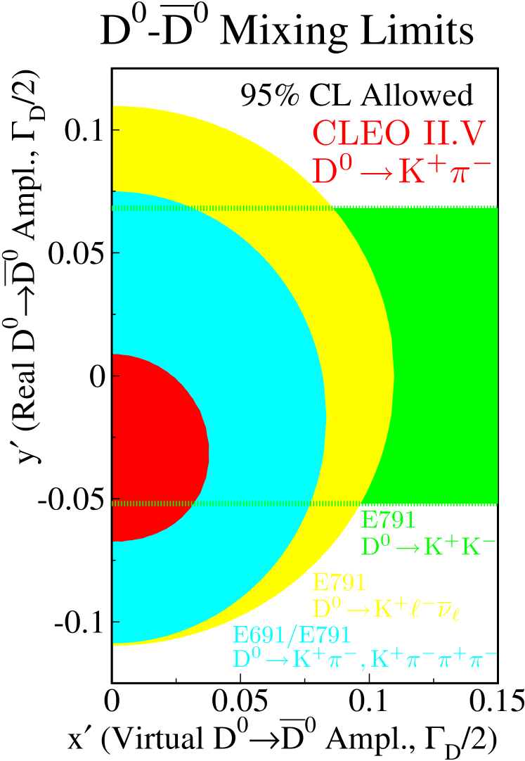
FIG. 11.: Limits in the $y^{\prime}$ v. $x^{\prime}$ plane. Our experiment limits, at 95% C.L., the true values of $x^{\prime}$ and $y^{\prime}$ to occupy the dark (red) region near the origin. Also shown are the similar zones from other recent experiments. We assume $\delta=0$ to place the recent work of E791 that utilized ${D^{0}}\!\to\!K^{+}K^{-}$; a non-zero $\delta$ would rotate the E791 confidence region clockwise about the origin by an angle of $\delta$.

Finally, if we assume that $\delta$ is small, which is plausible[8, 9], then $x^{\prime}\!\approx\!x$, and we can indicate the impact of our work in limiting predictions of ${D^{0}}\!-\!{\overline{D}\vrule width=0.0pt^{0}}$ mixing from extensions to the Standard Model. We plot our one-dimensional allowed region in $x^{\prime}$ in Fig. 12. Eighteen of the predictions tabulated in a paper contributed to this symposium[3] have some inconsistency with our limit. Among those predictions, some authors have made common assumptions, however.

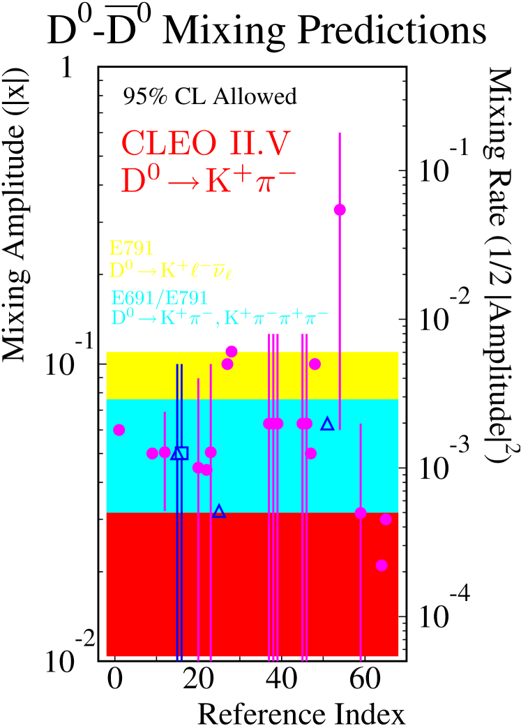
FIG. 12.: Predictions impacted by this work. The horizontal axis is the Reference Index used in [3], that corresponds to the reference tabulated there. The horizontal region (red) nearest the bottom is the allowed region, at 95% CL, consistent with this work, in the plausible approximation that $x^{\prime}\!=\!x$. There are 18 predictions that have some inconsistency with this work.

In conclusion, we conducted a study of the wrong-sign process, ${D^{0}}\!\to\!K^{+}\pi^{-}$, and conclusively established its rate, relative to the right-sign process, ${\overline{D}\vrule width=0.0pt^{0}}\to\!K^{+}\pi^{-}$, as $R_{\rm ws}=(0.34\pm 0.07\pm 0.06)\%$. By a study of that rate as a function of the decay time of the ${D^{0}}$, we distinguish the rate of direct, doubly-Cabibbo-suppressed decay ${D^{0}}\!\to\!K^{+}\pi^{-}$ relative to ${\overline{D}\vrule width=0.0pt^{0}}\!\to\!K^{+}\pi^{-}$, to be $R_{D}=(0.50^{+0.11}_{-0.12}\pm 0.08)\%$. The amplitudes that describe ${D^{0}}\!-\!{\overline{D}\vrule width=0.0pt^{0}}$ mixing, $x^{\prime}$ and $y^{\prime}$, are consistent with zero. The one-dimensional limits, at the 95% C.L., that we determine are $(1/2)x^{\prime 2}<0.05\%$, and $-5.9\%<y^{\prime}<0.3\%$. The limit on $x^{\prime}$, combined with the plausible assumption that the relative strong phase $\delta\!=\!0$, has some inconsistency with a variety of extensions to the Standard Model. Limits in the two-dimensional plane of $y^{\prime}$ versus $x^{\prime}$ are given in Fig. 11.

All results described here are preliminary.

We gratefully acknowledge the effort of the CESR staff in providing us with excelled luminosity and running conditions. We wish to acknowledge and thank the technical staff who contributed to the success of the CLEO II.V detector upgrade, including J. Cherwinka and J. Dobbins (Cornell); M. O’Neill (CRPP); M. Haney (Illinois); M. Studer and B. Wells (OSU); K. Arndt, D. Hale, and S. Kyre (UCSB). We appreciate contributions from G Lutz and advice from A. Schwarz. This work was supported by the National Science Foundation, The U.S. Department of Energy, Research Corporation, the Natural Sciences and Engineering Research Council of Canada, the A. P. Sloan Foundation, the Swiss National Science Foundation, and the Alexander von Humboldt Stiftung.

REFERENCES

- [1] M. Gell-Mann and A. Pais, Phys. Rev. 97, 1387 (1955).
-
[2]
S. L. Glashow, J. Illiopolous, and L. Maiani,
Phys. Rev. D 2, 1285 (1970);
R. L. Kingsley, S. B. Treiman, F. Wilczek, and A. Zee,
Phys. Rev. D 11, 1919 (1975). The latter paper contains
the following provocative observation:
‘Since charmed mesons will pretty surely have lifetimes too small to permit direct measurements of the kind that have been carried out in the , system, one can at best hope to get information on mixing only through indirect methods, by integrating count rates over time.’
- [3] For a compilation of predictions for , see H. N. Nelson, hep-ex/9908021, submitted to this Symposium.
- [4] C. Caso, et. al. European Physical Journal C 3 1 (1998).
- [5] A. Pais and S. B. Treiman, Phys. Ref. D 12, 2744 (1975).
- [6] E. Golowich and A. A. Petrov, Phys. Lett. B 427, 172 (1998).
- [7] I. I. Bigi, in Proceedings of the Beijing Charm Physics Symposium, edited by Ming-han Ye and Tao Huang, (Gordon and Breach Science Publishers, New York, 1987) pp. 339-425.
- [8] L. Wolfenstein, Phys. Rev. Lett. 75 2460 (1995).
- [9] T. E. Browder and S. Pakvasa, Phys. Lett. B 383, 475 (1996).
- [10] S. B. Treiman and R. G. Sachs, Phys. Rev. 103, 1545 (1956).
- [11] G. Blaylock, A. Seiden, and Y. Nir, Phys. Lett. B 355, 555 (1995).
- [12] Y. Kubota, Nucl. Instrum. Meth. A 320, 66 (1992).
- [13] T. S. Hill, Nucl. Instrum. Meth. A 418, 32 (1998).
- [14] G. Bonvicini et. al., Phys. Rev. Lett. 82, 4586 (1999).
- [15] L. Gibbons et. al., Phys. Rev. D56 3783 (1997).
- [16] D. Cinabro et. al., Phys. Rev. Lett. 72 1406 (1994).
- [17] R. Barate et. al., Phys. Lett. B 436 211 (1998).
- [18] E. M. Aitala et. al., Phys. Rev. D 57 13 (1998).
- [19] J. C. Anjos et. al., Phys. Rev. Lett. 60 1239 (1988).
- [20] D. Cinabro et. al., Phys. Rev. E 57, 1193 (1998).
- [21] R. Barlow, Nucl. Instrum. Meth. A 297, 496 (1990).
- [22] E. M. Aitala et. al., Phys. Rev. Lett. 77 2384, (1996).
- [23] E. M. Aitala et. al., Phys. Rev. Lett. 83 23, (1999).