Study of charmless hadronic B decays into the final states $K\pi,\pi\pi$, and $KK$, with the first observation of $B\to\pi^{+}\pi^{-}$ and $B\to K^{0}\pi^{0}$

Abstract

We have studied charmless hadronic decays of $B$ mesons into two-body final states with kaons and pions. We present preliminary results based on 9.66 million $B\bar{B}$ pairs collected with the CLEO detector. We have made the first observation of the decay $B\rightarrow\pi^{+}\pi^{-}$, with the branching fraction of $Br(B\rightarrow\pi^{+}\pi^{-})=(4.7^{+1.8}_{-1.5}\pm 0.6)\times 10^{-6}$. We have also observed for the first time the decay $B\rightarrow K^{0}\pi^{0}$ with the branching fraction of $Br(B\rightarrow K^{0}\pi^{0})=(14.8^{+5.9+2.4}_{-5.1-3.3})\times 10^{-6}$, thus completing the set of four $K\pi$ branching fraction measurements. We present improved measurements for the decays $B\to K^{\pm}\pi^{\mp}$, $B^{\pm}\to K^{0}\pi^{\pm}$, and $B^{\pm}\to K^{\pm}\pi^{0}$. We use these and other charmless hadronic B decays to make a first determination of the value of the weak phase ${\rm Arg}(V^{*}_{ub})=\gamma={113^{\circ}}^{+25^{\circ}}_{-23^{\circ}}$.

I Introduction

The phenomenon of $CP$ violation, so far observed only in the neutral kaon system, can be accommodated by a complex phase in the Cabibbo-Kobayashi-Maskawa (CKM) quark-mixing matrix [1]. Whether this phase is the correct, or only, source of $CP$ violation awaits experimental confirmation. $B$ meson decays, in particular charmless $B$ meson decays, will play an important role in verifying this picture.

The decay $B\rightarrow\pi^{+}\pi^{-}$, dominated by the $b\rightarrow u$ tree diagram (Fig. 1(a)), can be used to measure $CP$ violation due to $B^{0}-\bar{B}^{0}$ mixing at both asymmetric $B$ factories and hadron colliders. However, theoretical uncertainties due to the presence of the $b\to dg$ penguin diagram (Fig. 1(b)) make it difficult to extract the angle $\alpha$ of the unitarity triangle from $B\rightarrow\pi^{+}\pi^{-}$ alone. Additional measurements of $B^{\pm}\rightarrow\pi^{\pm}\pi^{0}$, $B,\bar{B}\rightarrow\pi^{0}\pi^{0}$, and the use of isospin symmetry may resolve these uncertainties [2].

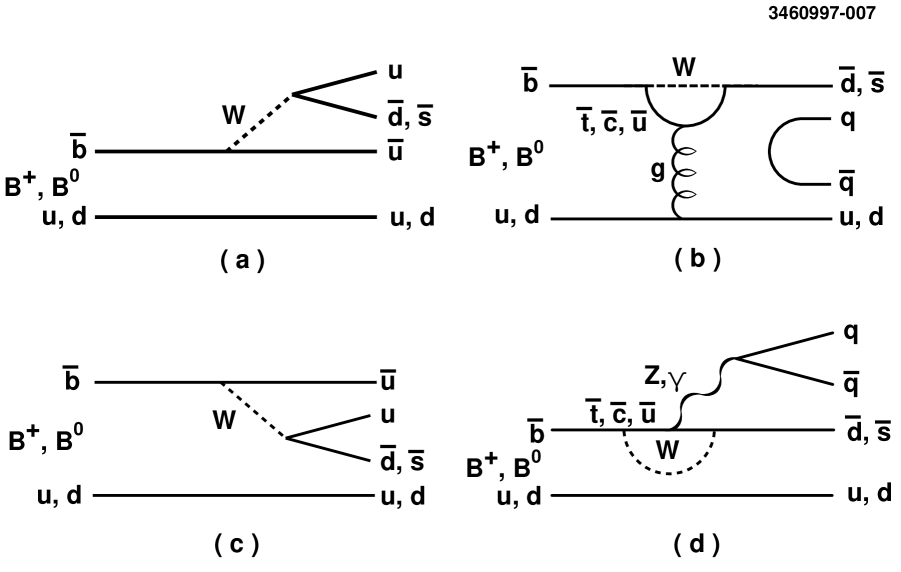
FIG. 1.: The dominant decay processes are expected to be (a) external W-emission, (b) gluonic penguin, (c) internal W-emission, (d) external electroweak penguin.

$B\to K\pi$ decays are dominated by the $b\rightarrow sg$ gluonic penguin diagram, with additional contributions from $b\rightarrow u$ tree and color-allowed electroweak penguin (Fig. 1(d)) processes. Interference between the penguin and tree amplitudes can lead to direct $CP$ violation, which would manifest itself as a rate asymmetry for decays of $B$ and $\bar{B}$ mesons. Several methods of measuring or constraining $\gamma$, the phase of $V_{ub}$. using only decay rates of $B\to K\pi,~{}\pi\pi$ processes were also proposed [3] [4] [5]. This is particularly important, as $\gamma$ is the least known parameter of the unitarity triangle and is likely to remain the most difficult to determine experimentally. This paper presents the first observation of the decays $B\to\pi^{+}\pi^{-}$ and $B\to K^{0}\pi^{0}$, improved measurements for $B\to K^{\pm}\pi^{\mp}$, $B^{\pm}\to K^{0}\pi^{\pm}$, and $B^{\pm}\to K^{\pm}\pi^{0}$ decays, and updated upper limits for $B$ decays to $\pi^{\pm}\pi^{0},~{}K^{+}K^{-}$, and $K^{0}K^{\pm}$. Average over charge conjugate decays is implied throughout this paper.

II Data Set, Detector, Event Selection

The data used in this analysis was collected with the CLEO II and CLEO II.V detectors at the Cornell Electron Storage Ring (CESR). It consists of $9.1~{}{\rm fb}^{-1}$ taken at the $\Upsilon$(4S) (on-resonance) and $4.5~{}{\rm fb}^{-1}$ taken below $B\bar{B}$ threshold. The below-threshold sample is used for continuum background studies. The on-resonance sample contains 9.66 million $B\bar{B}$ pairs. This is a $67\%$ increase in the number of $B\bar{B}$ pairs over the previously presented analysis [6].

CLEO II and CLEO II.V are general purpose solenoidal magnet detectors, described in detail elsewhere [7]. In CLEO II, the momenta of charged particles are measured in a tracking system consisting of a 6-layer straw tube chamber, a 10-layer precision drift chamber, and a 51-layer main drift chamber, all operating inside a 1.5 T superconducting solenoid. The main drift chamber also provides a measurement of the specific ionization loss, $dE/dx$, used for particle identification. For CLEO II.V the 6-layer straw tube chamber was replaced by a 3-layer double-sided silicon vertex detector, and the gas in the main drift chamber was changed from an argon-ethane to a helium-propane mixture. Photons are detected using 7800-crystal CsI(Tl) electromagnetic calorimeter. Muons are identified using proportional counters placed at various depths in the steel return yoke of the magnet.

Charged tracks are required to pass track quality cuts based on the average hit residual and the impact parameters in both the $r-\phi$ and $r-z$ planes. Candidate $K^{0}_{S}$ are selected from pairs of tracks forming well-measured displaced vertices. Furthermore, we require the $K^{0}_{S}$ momentum vector to point back to the beam spot and the $\pi^{+}\pi^{-}$ invariant mass to be within $10$ MeV, $\sim 2.5$ standard deviations ($\sigma$), of the $K^{0}_{S}$ mass. Isolated showers with energies greater than $40$ MeV in the central region of the CsI calorimeter and greater than $50$ MeV elsewhere, are defined to be photons. To reduce combinatoric backgrounds we require the lateral shapes of the showers to be consistent with those from photons. To suppress further low energy showers from charged particle interactions in the calorimeter we apply a shower energy dependent isolation cut. Pairs of photons with an invariant mass within $25$ MeV ($\sim 2.5\sigma$) of the nominal $\pi^{0}$ mass are kinematically fitted with the mass constrained to the $\pi^{0}$ mass.

Charged particles ($h^{\pm}$) are identified as kaons or pions using $dE/dx$. Electrons are rejected based on $dE/dx$ and the ratio of the track momentum to the associated shower energy in the CsI calorimeter. We reject muons by requiring that the tracks do not penetrate the steel absorber to a depth greater than seven nuclear interaction lengths. We have studied the $dE/dx$ separation between kaons and pions for momenta $p\sim 2.6$ GeV$/c$ in data using $D^{*+}$-tagged $D^{0}\rightarrow K^{-}\pi^{+}$ decays; we find a separation of $(1.7\pm 0.1)~{}\sigma$ for CLEO II and $(2.0\pm 0.1)~{}\sigma$ for CLEO II.V.

III Analysis

We calculate a beam-constrained $B$ mass $M=\sqrt{E_{\rm b}^{2}-p_{B}^{2}}$, where $p_{B}$ is the $B$ candidate momentum and $E_{\rm b}$ is the beam energy. The resolution in $M$ is dominated by the beam energy spread and ranges from 2.5 to 3.0 ${\rm MeV}/{\it c}^{2}$, where the larger resolution corresponds to decay modes with a $\pi^{0}$. We define $\Delta E=E_{1}+E_{2}-E_{\rm b}$, where $E_{1}$ and $E_{2}$ are the energies of the daughters of the $B$ meson candidate. The resolution on $\Delta E$ is mode dependent. For final states without $\pi^{0}$’s, the $\Delta E$ resolution for CLEO II(II.V) is $\pm 25(20)$ MeV. In the $B^{\pm}\to h^{\pm}\pi^{0}$ analysis the $\Delta E$ resolution is worse by approximately a factor of two and becomes asymmetric because of energy loss out of the back of the CsI crystals. The energy constraint also helps to distinguish between modes of the same topology. For example, $\Delta E$ for $B\rightarrow K^{+}\pi^{-}$, calculated assuming $B\rightarrow\pi^{+}\pi^{-}$, has a distribution that is centered at $-42$ MeV, giving a separation of $1.7(2.1)\sigma$ between $B\rightarrow K^{+}\pi^{-}$ and $B\rightarrow\pi^{+}\pi^{-}$ for CLEO II(II.V). We accept events with $M$ within $5.2-5.3$ $\rm{GeV/c^{2}}$ and $|\Delta E|<200(300)$ MeV for decay modes without (with) a $\pi^{0}$ in the final state. This fiducial region includes the signal region and a sideband for background determination.

We have studied backgrounds from $b\to c$ decays and other $b\to u$ and $b\to s$ decays and find that all are negligible for the analyses presented here. The main background arises from $e^{+}e^{-}\to q\bar{q}$ (where $q=u,d,s,c$). Such events typically exhibit a two-jet structure and can produce high momentum back-to-back tracks in the fiducial region. To reduce contamination from these events, we calculate the angle $\theta_{S}$ between the sphericity axis[8] of the candidate tracks and showers and the sphericity axis of the rest of the event. The distribution of $\cos\theta_{S}$ is strongly peaked at $\pm 1$ for $q\bar{q}$ events and is nearly flat for $B\bar{B}$ events. We require $|\cos\theta_{S}|<0.8$ which eliminates $83\%$ of the background. Using a detailed GEANT-based Monte-Carlo simulation [9] we determine overall detection efficiencies (${\cal E}$) of $11-45\%$, as listed in Table I. Efficiencies include the branching fractions for $K^{0}\to K^{0}_{S}\to\pi^{+}\pi^{-}$ and $\pi^{0}\to\gamma\gamma$ where applicable.

Additional discrimination between signal and $q\bar{q}$ background is provided by a Fisher discriminant technique as described in detail in Ref. [10]. The Fisher discriminant is a linear combination, ${\cal F}\equiv\sum_{i=1}^{N}\alpha_{i}y_{i}$, where the coefficients $\alpha_{i}$ are chosen to maximize the separation between the signal and background Monte Carlo samples. The 11 inputs, $y_{i}$, are the cosine of the angle between the candidate sphericity axis and beam axis, the ratio of Fox-Wolfram moments $H_{2}/H_{0}$ [12], and nine variables that measure the scalar sum of the momenta of tracks and showers from the rest of the event in nine angular bins, each of $10^{\circ}$, centered about the candidate’s sphericity axis.

We perform unbinned maximum-likelihood (ML) fits using $\Delta E$, $M$, ${\cal F}$, the angle between the $B$ meson momentum and beam axis, and $dE/dx$ (where applicable) as input information for each candidate event to determine the signal yields. Four different fits are performed, one for each topology ($h^{+}h^{-}$, $h^{\pm}\pi^{0}$, $h^{\pm}K^{0}_{S}$, and $K^{0}_{S}\pi^{0}$, $h^{\pm}$ referring to a charged kaon or pion). In each of these fits, the likelihood of the event is parameterized by the sum of probabilities for all relevant signal and background hypotheses, with relative weights determined by maximizing the likelihood function ($\cal L$). The probability of a particular hypothesis is calculated as a product of the probability density functions (PDFs) for each of the input variables. Further details about the likelihood fit can be found in Ref. [10]. The parameters for the PDFs are determined from independent data and high-statistics Monte Carlo samples. We estimate a systematic error on the fitted yield by varying the PDFs used in the fit within their uncertainties. These uncertainties are dominated by the limited statistics in the independent data samples we used to determine the PDFs. The systematic errors on the measured branching fractions are obtained by adding this fit systematic in quadrature with the systematic error on the efficiency.

IV Results

We summarize all branching fractions and upper limits in Table I. We find statistically significant signals for the decays $B\to K^{\pm}\pi^{\mp}$, $B\to\pi^{+}\pi^{-}$, $B^{\pm}\to K^{\pm}\pi^{0}$, $B^{\pm}\to K^{0}_{S}\pi^{\pm}$, and $B\to K^{0}_{S}\pi^{0}$.

TABLE I.: Experimental results. Branching fractions (${\cal B}$) and 90% C.L. upper limits are given in units of $10^{-6}$. The errors on ${\cal B}$ are statistical and systematics respectively. Reconstruction efficiency ${\cal E}$ includes branching fractions of $K^{0}\to K^{0}_{S}\to\pi^{+}\pi^{-}$ and $\pi^{0}\to\gamma\gamma$. We quote the central value branching fraction in $\pi^{\pm}\pi^{0}$ for convenience only. The statistical significance of the excess above background in this final state is insufficient for a first observation of this decay mode.

Mode	${\cal E}(\%)$	${\cal B}_{fit}$($10^{-6}$)	Signif.(std.dev.)	${\cal B}$($10^{-6}$)
$\pi^{+}\pi^{-}$	$45$	$4.7^{+1.8}_{-1.5}$	4.2	$4.7^{+1.8}_{-1.5}\pm 0.6$
$\pi^{+}\pi^{0}$	$41$	$5.4^{+2.1}_{-2.0}\pm 1.5$	3.2	$<12$
$K^{+}\pi^{-}$	$45$	$18.8^{+2.8}_{-2.6}$	11.7	$18.8^{+2.8}_{-2.6}\pm 1.3$
$K^{+}\pi^{0}$	$38$	$12.1^{+3.0}_{-2.8}$	6.1	$12.1^{+3.0+2.1}_{-2.8-1.4}$
$K^{0}\pi^{+}$	$14$	$18.2^{+4.6}_{-4.0}$	7.6	$18.2^{+4.6}_{-4.0}\pm 1.6$
$K^{0}\pi^{0}$	$11$	$14.8^{+5.9}_{-5.1}$	4.7	$14.8^{+5.9+2.4}_{-5.1-3.3}$
$K^{+}K^{-}$	$45$		0.	$<2.0$
$K^{+}\bar{K}^{0}$	$14$		1.1	$<5.1$

Fig. 2 shows the results of the likelihood fit for $B\to\pi^{\pm}\pi^{\mp}$ and $B\to K^{\pm}\pi^{\mp}$. The curves represent the $n\sigma$ contours, which correspond to the increase in $-2\ln{\cal L}$ by $n^{2}$. The dashed curve marks the $3\sigma$ contour; systematic uncertainties are not included in any contour plots. The statistical significance of a given signal yield is determined by repeating the fit with the signal yield fixed to be zero and recording the change in $-2\ln{\cal L}$. Fig. 3 shows distributions in $M$ and $\Delta E$ for events after cuts on the Fisher discriminant and whichever of $M$ and $\Delta E$ is not being plotted, plus an exclusive classification into $K\pi$-like and $\pi\pi$-like candidates based on the most probable assignment with $dE/dx$ information. The likelihood fit, suitably scaled to account for the efficiencies of the additional cuts, is overlaid in the $\Delta E$ distributions to illustrate the separation between $K\pi$ and $\pi\pi$ events.

FIG. 2.: Contours of the $-2\ln{\cal L}$ for the ML fit to $N_{K^{\pm}\pi^{\mp}}$ and $N_{\pi^{+}\pi^{-}}$, the $K^{\pm}\pi^{\mp}$ and $\pi^{+}\pi^{-}$ yields respectively.

FIG. 3.: Projections of $K\pi$ and $\pi\pi$ events onto $M$ and $\Delta E$ with cuts. Upper left: $M$ distribution of $K\pi$-like events; upper right: $M$ distribution of $\pi\pi$-like events. Lower left: $\Delta E$ distribution of events prior to $\pi\pi$ vs $K\pi$ vs $KK$ selection according to dE/dx; Lower right: $\Delta E$ distribution of events that are more likely to be $\pi\pi$ than $K\pi$ or $KK$ based on dE/dx. Overlays in the lower plots are the results of the likelihood fit scaled by the efficiency of the cuts used to project into these plots. Solid line: total fit; dashed: $K\pi$; dotted: $\pi\pi$; dot-dash: continuum background.

We also compute from the PDFs the event-by-event probability to be signal or continuum background, and also the probability to be $K\pi$-like or $\pi\pi$-like. From these we form likelihood ratios, ${\cal R}_{sig}=(P^{s}_{\pi\pi}+P^{s}_{K\pi})/(P^{s}_{\pi\pi}+P^{s}_{K\pi}+P^{c}_{\pi\pi}+P^{c}_{K\pi}+P^{c}_{KK})$ and ${\cal R}_{\pi}=P^{s}_{\pi\pi}/(P^{s}_{\pi\pi}+P^{s}_{K\pi})$. Superscript $s$ and $c$ stand for signal and continuum background respectively. Fig. 4 illustrates the distribution of events in ${\cal R}_{sig}$ (vertical axis) and ${\cal R}_{\pi}$ (horizontal axis). Signal events cluster near the top of the figure, and separate into $K\pi$-like events on the left and $\pi\pi$-like events on the right.

We find no evidence for the decay $B\to K^{\pm}K^{\mp}$ and set an upper limit accordingly, as shown in Table I.

FIG. 4.: The horizontal axis shows $P^{s}_{\pi\pi}/(P^{s}_{\pi\pi}+P^{s}_{K\pi})$ while the vertical axis depicts $(P^{s}_{\pi\pi}+P^{s}_{K\pi})/(P^{s}_{\pi\pi}+P^{s}_{K\pi}+P^{c}_{\pi\pi}+P^{c}_{K\pi}+P^{c}_{KK})$. Superscript $s$ and $c$ stand for signal and continuum background, respectively. Signal events cluster near the top of the figure, and separate into $K\pi$-like events on the left and $\pi\pi$-like events on the right.

The results of the $K_{S}\pi^{0}$ fit are shown in Fig. 5. The signal yield of $15.5^{+5.9}_{-5.0}$ events is 4.7$\sigma$ significant and robust under variations of cuts and PDF parameter variations.

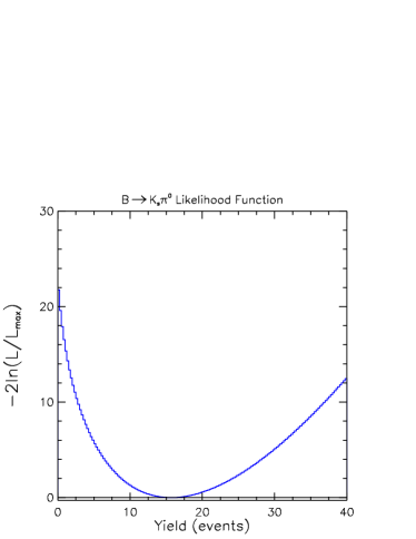
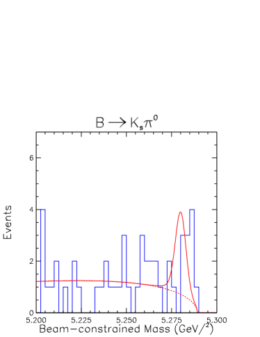
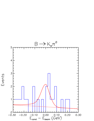
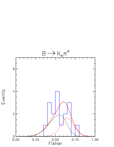
FIG. 5.: $B\to K_{S}\pi^{0}$: Upper left: Likelihood function versus $K_{S}\pi^{0}$ yield; Upper right: projection onto $M$ axis (efficiency = 0.63); Lower left: projection onto $\Delta E$ axis (efficiency = 0.63); Lower right: projection onto ${\cal F}$ axis (efficiency = 0.69). Overlaid curves are the results of the likelihood fit, scaled according to the efficiency of the projection cuts. Solid: total fit; dotted: continuum background; dashed: signal.

Figures 6 and 7 illustrate contour plots of $-2\ln{\cal L}$ for the ML fit to $K^{0}_{s}h^{\pm}$ and $h^{\pm}\pi^{0}$. The branching ratios and limits associated with these four fits are given in Table I. We also show projections onto $M$ and $\Delta E$ for these modes in Figures 8 and 9.

FIG. 6.: Contours of the $-2\ln{\cal L}$ for the ML fit to $N_{K^{0}_{S}\pi^{\pm}}$ and $N_{K^{0}_{S}K^{\pm}}$.

FIG. 7.: Contours of the $-2\ln{\cal L}$ for the ML fit to $N_{K^{\pm}\pi^{0}}$ and $N_{\pi^{\pm}\pi^{0}}$.

FIG. 8.: $B\to K_{S}\pi^{\pm}$. Projections onto $M$ (top) and $\Delta E$ (bottom) in GeV. Cuts are made on the Fisher discriminant and whichever of $M$ and $\Delta E$ is not being plotted.

FIG. 9.: $B\to K^{\pm}\pi^{0}$. Projections onto $M$ (left) and $\Delta E$ (right). Cuts are made on the Fisher discriminant and whichever of $M$ and $\Delta E$ is not being plotted.

To evaluate how systematic uncertainties in the PDFs affect the statistical significance for modes where we claim first observations, we repeated the fits for the $h^{+}h^{-}$ and $K^{0}_{S}\pi^{0}$ modes with all PDFs changed simultaneously within their uncertainties to maximally reduce the signal yield in the modes of interest. Under these extreme conditions, the significance of the first-observation modes $\pi^{+}\pi^{-}$ and $K^{0}_{S}\pi^{0}$ becomes $3.2$ and $3.8~{}\sigma$ respectively. We also evaluate the branching ratios with alternative analyses using tighter and looser cuts on the continuum suppressing variable $|\cos\theta_{S}|$. These variations correspond to halving and doubling the background in the fitted sample. The branching ratios change under these variations by much less than the statistical error.

The fitted yields in the remaining modes are not statistically significant. We calculate $90\%$ confidence level (C.L.) upper limit yields by integrating the likelihood function

$${\int_{0}^{N^{UL}}{\cal L}_{\rm max}(N)dN\over\int_{0}^{\infty}{\cal L}_{\rm max}(N)dN}=0.90$$ (1)

where ${\cal L}_{\rm max}(N)$ is the maximum $\cal L$ at fixed $N$ to conservatively account for possible correlations among the free parameters in the fit. We then increase upper limit yields by their systematic errors and reduce detection efficiencies by their systematic errors to calculate branching fraction upper limits given in Table I.

V Information on the Weak Phase $\gamma$

Charmless hadronic $B$ decays are a sensitive probe of $\gamma$, the phase of the CKM matrix element $V_{ub}^{*}$, due to the interference of tree (Fig. 1(a)) and penguin (Fig. 1(b)) diagrams. A number of methods for extracting $\gamma$ from these decays have been proposed, relying on either the construction of amplitude triangles[3], or ratios of CP-averaged branching fractions[4][5]. While some of these methods have the virtue of being independent of model assumptions about strong interaction effects[5], none of them provide useful constraints on $\gamma$ given the present level of precision of our data, as they use only a restricted set of measurements.

Alternatively, one may trade model independence against exhaustive use of the available data and attempt a model dependent fit to a large number of measurements. Such a fit is described in detail in Ref. [14]. In this section we will briefly describe the basic ideas, as well as the main results of this work.

As pointed out in a recent paper by He, Hou, and Yang,[15] a number of CLEO measurements of charmless hadronic $B$ decays indicate a preferance for $\cos\gamma<0.0$. This conclusion is based on a comparison of the CP-averaged branching fraction measurements with theoretical predictions based on the factorization model. In this section we report results of a global fit that quantifies the qualitative observation made in Ref. [15].

Assuming factorization one may express[16][17] the decay amplitudes in terms of CKM matrix elements, form factors, decay constants, quark and meson masses, short distance coefficients, etc. Many of these are known to more than adequate precision. In addition, one may relate many of the poorly known quantities assuming unitarity of the CKM matrix as well as relationships among form factors. As a result, only five poorly known parameters are needed to predict CP averaged branching fractions for many of the CLEO measurements on charmless hadronic $B$ decays. These parameters are:

$$\begin{array}[]{ccc}\gamma&=&Arg(V_{ub}^{*})\\ |V_{ub}/V_{cb}|&&\\ R_{su}&=&{2m_{K}^{2}\over(m_{b}-m_{u})(m_{s}+m_{u})}\sim{2m_{K}^{2}\over m_{b}\times m_{s}}\\ F^{B\to\pi}&=&B\to\pi\ \mathrm{transitions\ form\ factor}\\ A^{B\rho}_{0}&=&B\to\rho\ \mathrm{transitions\ form\ factor}\\ \end{array}$$ (2)

We then form a $\chi^{2}$ between the CLEO results [13] for the final states $K^{\pm}\pi^{\mp},\ K^{\pm}\pi^{0},\ K^{0}_{s}\pi^{\pm},\ K^{0}_{s}\pi^{0},\ \pi^{+}\pi^{-},\ \pi^{\pm}\pi^{0},\ \rho^{0}\pi^{\pm},\ \omega\pi^{\pm},\ \rho^{\pm}\pi^{\mp},\ K^{*\pm}\pi^{\mp},\ \omega K^{0}_{s},\ \omega K^{\pm},\ \phi K^{0}_{s},\ \phi K^{\pm}$ and the theoretical predictions for the respective CP-averaged branching fractions. As additional constraint we add $|V_{ub}/V_{cb}|=0.08\pm 0.02$, thus arriving at a $15-5$ degree of freedom fit. We should note that only 9 of the 14 decay modes are unambiguously observed (i.e. with statistical significances of more than 4 standard deviations). For the remaining 5 final states we see excess yields above background expectations that have statistical significances ranging from $\sim 1.5$ to close to $4$ standard deviations.

Our choice of decay modes to include was dictated by the following rationale. We consider for inclusion all decay modes with final states containing two pseudo-scalars, or a pseudo-scalar and a vector meson, for which we have results presented at this conference. We then exclude final states with $\eta$ and $\eta^{\prime}$ due to the known ambiguities in predicting these decays [18]. We furthermore exclude all final states for which the factorization model makes predictions that are well below the sensitivity of our present data.

Minimizing the resulting $\chi^{2}$ we find a global minimum of $10.3$ for $10$ degrees of freedom. The parameters at the minimum are:

$$\begin{array}[]{ccc}\gamma&=&113^{+25}_{-23}\ (161)~{}\mathrm{degrees}\\ |V_{ub}/V_{cb}|&=&0.082\pm 0.017\ (0.062)\\ R_{su}&=&1.7\pm 0.4\ (0.57)\\ F^{B\to\pi}&=&0.27^{+0.05}_{-0.04}\ (0.43)\\ A_{0}^{B\to\rho}&=&0.52^{+0.16}_{-0.12}\ (0.78)\\ \end{array}$$ (3)

The central value for $R_{su}$ corresponds to $m_{s}(m_{b}=4.34$GeV$)$ of about $66$ MeV. The numbers in parentheses are the values for a second local minimum with only marginally larger $\chi^{2}$. These are the only minima found while repeating the fit $200$ times with random starting points across a large volume in the five dimensional parameter space.

Figure 10 shows the dependence of $\chi^{2}$ versus $\gamma$. We refit at each value of $\gamma$ to allow the fit to find the global minimum at each fixed value of $\gamma$. This is important as the correlation matrix for the five free parameters has significant off-diagonal elements. For example, the two most correlated parameters are $|V_{ub}/V_{cb}|$ and $A_{0}^{B\to\rho}$ with a correlation coefficient of $-0.8$.

We note that the best fit values for all parameters are closely consistent with theoretical expectations [16] [17] [19]. This is either a surprising coincidence or an indication that the model provides an adequate description of nature. If we were to believe the latter than we would have to conclude that we have made a meaningful measurement of $\gamma$, the phase of $V_{ub}^{*}$.

FIG. 10.: $\chi^{2}$ versus $\gamma$ curve for global fit to CP-averaged charmless hadronic $B$ decay branching fractions. The triangles depict a local minimum that has the feature of $m_{s}=218$MeV. The squares depict the $\chi^{2}$ curve with the additional constraint of $m_{s}<150$MeV.

VI Summary

In summary, we have measured branching fractions for all four exclusive $B\to K\pi$ decays and made first observations of the decays $B\to\pi^{+}\pi^{-}$ and $B\to K^{0}\pi^{0}$. The latter observation completes the full set of $B\to K\pi$ measurements. In addition, we have shown that a global fit to CP-averaged branching fractions measured by CLEO allows for a model dependent measurement of $\gamma=113^{+25}_{-23}$ degrees. This is the first determination of the complex phase of the CKM matrix by any method other than the unitarity triangle construction.

VII Acknowledgements

We gratefully acknowledge the effort of the CESR staff in providing us with excellent luminosity and running conditions. J.R. Patterson and I.P.J. Shipsey thank the NYI program of the NSF, M. Selen thanks the PFF program of the NSF, M. Selen and H. Yamamoto thank the OJI program of DOE, J.R. Patterson, K. Honscheid, M. Selen and V. Sharma thank the A.P. Sloan Foundation, M. Selen and V. Sharma thank the Research Corporation, F. Blanc thanks the Swiss National Science Foundation, and H. Schwarthoff and E. von Toerne thank the Alexander von Humboldt Stiftung for support. This work was supported by the National Science Foundation, the U.S. Department of Energy, and the Natural Sciences and Engineering Research Council of Canada.

REFERENCES

- [1] M. Kobayashi and K. Maskawa, Prog. Theor. Phys. 49, 652 (1973).
- [2] M. Gronau and D. London, Phys. Rev. Lett. 65, 3381 (1990).
- [3] M. Gronau, J. L. Rosner, and D. London, Phys. Rev. Lett. 73, 21 (1994); R. Fleischer, Phys. Lett. B 365, 399 (1996);
- [4] R. Fleischer and T. Mannel, Phys. Rev. D 57, 2752 (1998).
- [5] M. Neubert and J. Rosner, Phys. Lett. B441, 403 (1998); M. Neubert, JHEP 9902, 14 (1999).
-
[6]
CLEO conference reports 98-09 (ICHEP98 860) and 98-20 (ICHEP98 858)
may be found at http://www.lns.cornell.edu/public/CONF/1998/CONF98-09/
and http://www.lns.cornell.edu/public/CONF/1998/CONF98-20/ respectively. - [7] Y. Kubota et al. (CLEO Collaboration), Nucl. Instrum. Methods Phys. Res., Sec. A320, 66 (1992); T. Hill, 6th International Workshop on Vertex Detectors, VERTEX 97, Rio de Janeiro, Brazil.
- [8] S. L. Wu, Phys. Rep. C107, 59 (1984).
- [9] R. Brun et al., GEANT 3.15, CERN DD/EE/84-1.
- [10] D. M. Asner et al. (CLEO Collaboration), Phys. Rev. D 53, 1039 (1996).
- [11] R. Godang et al. (CLEO Collaboration), Phys. Rev. Lett. 80, 3456 (1998); B. H. Behrens et al. (CLEO Collaboration), Phys. Rev. Lett. 80, 3710 (1998); D. M. Asner et al. (CLEO Collaboration), Phys. Rev. D 53, 1039 (1996).
- [12] G. Fox and S. Wolfram, Phys. Rev. Lett. 41, 1581 (1978).
- [13] CLEO CONF 99-13 (hep-ex/9908018) in addition to the present paper.
- [14] Wei-Shou Hou, J. G. Smith, F. Würthwein, in preparation.
- [15] Xiao-Gang He, Wei-Shu Hou, Kwei-Chou Yang, Phys. Rev. Lett. 83, 1100 (1999); Wei-Shu Hou, Kwei-Chou Yang, hep-ph/9908202.
- [16] Y.H. Chen et al., hep-ph/9903453, to appear in Phys. Rev. D.
- [17] A. Ali, G. Kramer, and C. Lü, Phys. Rev. D 58, (1998) 094009.
- [18] CLEO CONF 99-12 (hep-ex/9908019).
- [19] P. Ball and V.M. Braun, Phys. Rev. D58, 094016 (1998); P. Ball, J. High Energy Phys. 9809, 005 (1998).