Abstract

We present new results based on the entire CHOOZ data sample. We find (at 90 % confidence level) no evidence for neutrino oscillations in the $\bar{\nu}_{e}$ disappearance mode, for the parameter region given by approximately $\delta m^{2}>7\cdot 10^{-4}\hbox{$\,{\rm eV^{2}}$}$ for maximum mixing, and ${\rm sin}^{2}2\theta=0.10$ for large $\delta m^{2}$. Lower sensitivity results, based only on the comparison of the positron spectra from the two different-distance nuclear reactors, are also presented; these are independent of the absolute normalization of the $\bar{\nu}_{e}$ flux, the cross section, the number of target protons and the detector efficiencies.

Keywords: reactor, neutrino mass, neutrino mixing, neutrino oscillations

1 Introduction

Preliminary results of the CHOOZ experiment have already been published[1]. We present here the new results based on the entire data sample; they include a large increase in statistics and a better understanding of systematic effects.

The reader is refered to the previous article for an introduction to the problem of neutrino oscillations, for a general description of the experiment and for a discussion of its data analysis.

As the experiment progressed, calibration methods and stability checks were considerably refined, and knowledge of the apparatus’ behaviour and simulation by the Montecarlo method were improved As a consequence, systematic errors were considerably reduced.

Three results are given. The main one is based on all the available information: the measured number of positron events as a function of energy, separately obtained from each reactor. It uses the two spectral shapes, as well as the absolute normalizations. The second result is based only on the comparison of the positron spectra from the two, different-distance reactors. This analysis is largely unaffected by the absolute value of the $\bar{\nu}_{e}$ flux, the cross section, the number of target protons and the detector efficiencies, and is therefore dominated by statistical errors. The sensitivity in this case is limited to $\delta m^{2}\,\lower 2.15277pt\hbox{$\buildrel>\over{\sim}$}\,2\cdot 10^{-3}\hbox{$\,{\rm eV^{2}}$}$ due to the small distance, $\Delta L=116.7$ m, between the reactors. The explored $(\delta m^{2},\sin^{2}2\theta)$ parameter space still matches well the region of the atmospheric neutrino anomaly. The third analysis is similar to the first, but does not include the absolute normializations. All results were derived following the suggestions by Feldman & Cousins [4] .

2 Experimental data

The Chooz power station has two pressurized-water reactors with a total thermal power of $8.5\,{\,\rm{GW}}_{th}$. The first reactor reached full power in May $1997$, the second in August $1997$. A summary of our data taking (from April 7, 1997 to July 20, 1997) is presented in Table 1.

Table 1: Summary of the Chooz data acquisition cycle from April $1997$ to July $1998$.

	Time (h)	$\int W{\rm\,d}t$ ( GWh)
Run	8761.7
Live time	8209.3
Dead time	552.4
Reactor 1 only ON	2058.0	8295
Reactor 2 only ON	1187.8	4136
Reactors 1 & 2 ON	1543.1	8841
Reactors 1 & 2 OFF	3420.4

Note that the schedule was quite convenient for separating the individual reactor contributions and for determining the reactor-OFF background.

In this exepiment the $\bar{\nu}_{e}$’s are detected via the inverse $\beta$-decay reaction

$$\bar{\nu}_{e}+\rm p\rightarrow\rm e^{+}+\rm n$$

The $\bar{\nu}_{e}$ reaction signature is a delayed coincidence between the prompt $\rm e^{+}$ signal (boosted by the two 511-$\,{\rm keV}$ annihilation $\gamma$ rays), later called “primary signal”, and the signal due to the neutron capture in the Gd-loaded scintillator ($\gamma$-ray energy release $\sim 8\hbox{$\,{\rm MeV}$}$), later called “secondary signal”. During the experiment $1.2\times 10^{7}$ events were recorded on disk; weak selection criteria, based on the total charge measured by the PMT’s for the secondary signal, reduced this number to $7\times 10^{5}$ events, which were fully reconstructed in energy and in space. After applying the criteria for selecting $\nu$-interactions, we were left with $2991$ bona-fide candidates, including $287$ events from reactor-OFF periods.

2.1 Detector stability

During our approximately one year of data taking, the detector slowly varied its response due to the decrease of the optical clarity of the Gd-loaded scintillator (the scintillator emission was stable, but the light at the PMT’s exponentially decreased, with a time constant $\tau\sim 750\hbox{$\,{\rm d}$}$). This produced small effects on the trigger threshold and rate, the event reconstruction, the signal/background separation and the background level. While hardware thresholds were readjusted every few months, the detector response was checked daily by ${}^{60}\mbox{Co}$, ${}^{252}\mbox{Cf}$ and Am/Be sources, which provide $\gamma$-signals, neutron signals, and time correlated $\gamma-\rm n$ signals. The reconstruction of these event samples, the study of their time evolution, and the comparison with Montecarlo method predictions, permitted a thorough understanding of the detector behaviour and a precise evaluation of the small efficiency variations on neutrino-induced and background events. Figure 1 shows calibration data using the ${}^{252}\mbox{Cf}$ source at the detector center; the neutron capture lines ($2.2\hbox{$\,{\rm MeV}$}$ on hydrogen and $8\hbox{$\,{\rm MeV}$}$ on gadolinium) are compared with Montecarlo predictions. Position and energy resolutions are $\sigma_{x}=17.5\hbox{$\,{\rm cm}$}$ and $\sigma_{E}/E=5.6\,\%$ for n-captures releasing $8\hbox{$\,{\rm MeV}$}$. Calibrations at other locations always produced detector response in good agreement with the Montecarlo predictions.

Figure 1: Visible energy and position distributions of ²⁵²Cf source calibration data (at the detector center): comparison between data and Monte Carlo simulation.

Interestingly, we are sensitive to the two-line structure of the gadolinium capture at $8\hbox{$\,{\rm MeV}$}$. A fit to the data gives line energies and intensities of $7.77\hbox{$\,{\rm MeV}$}\quad(77\,\%)$ for ${}^{157}\mbox{Gd}$ and $8.31\hbox{$\,{\rm MeV}$}\quad(23\,\%)$ for ${}^{155}\mbox{Gd}$. The quality of the fit is good ($\chi^{2}=67.6$ with 55 dof); a single-Gaussian fit gives a much poorer result ($\chi^{2}=875$ with 58 dof).

As a demonstration of the excellent stability of the detector response, Fig. 2 shows the time evolution of the measured energy correponding to the $8\hbox{$\,{\rm MeV}$}$ capture line and the shape and width of this line, for spallation neutrons generated by cosmic ray muons during the entire duration of the experiment. Since these events occured everywhere in the detector, the data in Fig. 2 depends on daily calibrations, on the determination of all PMT and electronic channel amplification constants, on the knowledge of the scintillator attenuation length and its time evolution, and on the event reconstruction algorithms. The measured energy is somewhat lower than $8\hbox{$\,{\rm MeV}$}$, due to scintillator saturation effects and neutron-capture $\gamma$-ray leakage.

Figure 2: Position of the peak (left) and lineshape (right) of the $8\hbox{$\,{\rm MeV}$}$ $\gamma$-line.

2.2 Event Typology

A good understanding of the nature of the neutrino candidates can be obtained by viewing the events on a two-dimensional plot of “n-signal energy” vs. “$\rm e^{+}$-signal energy”, for reactor-ON (Fig. 3 (left)) and reactor-OFF (Fig. 3 (right)) data; no signal selection has yet been applied.

Figure 3: “n-signal energy” vs. “$\rm e^{+}$-signal energy” during the reactor-ON (left) and reactor-OFF (right) period; no selection applied.

One can observe four regions: A,B,C,D and the neutrino event window at the crossing of regions A and C. Regions B and C are filled by primary-secondary correlated signals. Region B contains stopping muons, i.e.: cosmic $\mu$’s which entered the detector through the small dead space (detector filling pipes, support flanges, etc.) missing the anticoincidence shield. These events have large primary energy and large secondary energies associated with the $\mu$-decay electrons. Events in region B have a secondary delay distribution in agreement with the $\mu$-lifetime at rest (see Fig. 4B).

Figure 4: Delay distribution of secondary events in the various regions.

Region C events are due to fast neutrons from nuclear spallations by cosmic rays in the rock and concrete surrounding the detector; these neutrons scatter and the recoil proton is detected as “primary”, while the neutron is thermalized and later captured as the “secondary” giving the characteristic $8\hbox{$\,{\rm MeV}$}$ capture energy; this fast neutron region overlaps the neutrino candidate region and is the main background source for the experiment. The secondary delay distribution is as expected for thermal neutron capture in the Gd-doped scintillator (the best-fit lifetime is $\tau=30.5\,\pm\,1\hbox{$\,{\rm\mu s}$}$) (see Fig. 4C). Regions A and D are filled by accidental events; region D events are due to the accidental coincidence (within $100\hbox{$\,{\rm\mu s}$}$) of two low energy natural radioactivity signals; region A events are due to an accidental coincidence of a low energy natural radioactivity signal and a high energy recoil proton from a fast neutron scattering. Both A and D delay distributions are flat, as expected (see Fig. 4A and D).

The definition of a neutrino event is based on the following requirements:

• energy cuts on the neutron candidate ($6-12\hbox{$\,{\rm MeV}$}$) and on the $\rm e^{+}$ candidate (from the threshold energy $E_{thr}\sim 1.3\hbox{$\,{\rm MeV}$}$ to $8\hbox{$\,{\rm MeV}$}$),

• a time window on the delay between the $e^{+}$ and the neutron ($2-100\hbox{$\,{\rm\mu s}$}$),

• spatial selections on the $\rm e^{+}$ and the neutron positions (distance from the PMT wall $>30\hbox{$\,{\rm cm}$}$ and distance between $\rm n$ and $\rm e^{+}<100\hbox{$\,{\rm cm}$}$),

• only one pulse satisfying the criteria for a secondary signal (neutron).

The application of these selection criteria (apart from energy selections) produces the two-dimensional plots of Fig. 5, for reactor-ON (left) and for reactor-OFF (right) data.

Figure 5: “n-signal energy” vs. “$\rm e^{+}$-signal energy” for reactor-ON (left) and reactor-OFF (right) data; selections other than energy applied.

One can clearly see that the events spilling into the neutrino event window are mainly those from region C (proton recoils and neutron capture from spallation fast neutrons) and, to a lesser extent, those from region D (two low energy natural radioactivity signals).

The effects of the selection criteria used to define the neutrino interactions were extensively studied by the Montecarlo method and by ad-hoc $\gamma$ and $n$-source calibrations. Similarly, we investigated the small edge effects associated with the acrylic vessel containing the Gd-loaded scintillator target. In Table 2 we present the efficiencies associated with the selection criteria and their errors.

Table 2: Summary of the neutrino detection efficiencies.

selection	efficiency $(\%)$	error $(\%)$
positron energy	$97.8$	$0.8$
positron-geode distance	$99.85$	$0.1$
neutron capture	$84.6$	$0.85$
capture energy containment	$94.6$	$0.4$
neutron-geode distance	$99.5$	$0.1$
neutron delay	$93.7$	$0.4$
positron-neutron distance	$98.4$	$0.3$
secondary multiplicity	$97.4$	$0.5$
combined	$69.8$	$1.1$

2.3 Positron spectrum

The measured positron spectrum for all reactor-ON data, and the corresponding reactor-OFF spectrum, are shown in Fig. 6.

Figure 6: Positron energy spectra in reactor-ON and OFF periods.

After background subtraction, the measured positron spectrum can be compared with the expected neutrino-oscillated positron spectrum at the detector position. For a mean reactor-detector distance $L_{k}$, this is given by:

$$\begin{split}S_{k}(E,L_{k},\theta,\delta m^{2})&=\frac{1}{4\pi L_{k}^{2}}n_{p}\int h(L,L_{k})\int\sigma(E_{\nu})S(E_{\nu})\times\\ &\quad P(E_{\nu},L,\theta,\delta m^{2})r(E_{e^{+}},E)\varepsilon(E_{e^{+}}){\rm\,d}E_{e^{+}}{\rm\,d}L,\end{split}$$ (1)

where

$E_{\nu},E_{e^{+}}$	are related by $E_{\nu}=E_{e^{+}}+(M_{n}-M_{p})+O(E_{\nu}/M_{n})$,
$n_{p}$	is the total number of target protons,
$\sigma(E_{\nu})$	is the neutrino cross section,
$S(E_{\nu})$	is the antineutrino spectrum,
$h(L,L_{k})$	is the spatial distribution function for the
	finite core and detector sizes,
$r(E_{e^{+}},E)$	is the detector response function linking
	the visible energy $E$ and the real positron energy $E_{e^{+}}$,
$\varepsilon(E_{e^{+}})$	is the neutrino detection efficiency,
$P(E_{\nu},L,\theta,\delta m^{2})$	is the two-flavour survival probability.

The $\bar{\nu}_{e}$ spectrum was determined, for each fissile isotope, by using the $\bar{\nu}_{e}$ yields obtained by conversion of the $\beta^{-}$-spectra measured at ILL [2]; these spectra were then renormalized according to the measurement of the integral $\bar{\nu}_{e}$ flux performed at Bugey[3]. The expected, non-oscillated positron spectrum was computed using the Monte Carlo codes to simulate both reactors and the detector. The resulting spectrum, summed over the two reactors, is superimposed on the measured one in Fig. 7 to emphasize the agreement of the data with the no-oscillation hypothesis. The Kolmogorov-Smirnov test for the compatibility of the two distributions gives an $82\,\%$ probability.

Figure 7: (above) Expected positron spectrum for the case of no oscillations, superimposed on the measured positron spectrum obtained from the subtraction of reactor-ON and reactor-OFF spectra; (below) measured vs. expected ratio. The errors shown are statistical.

The measured vs. expected ratio, averaged over the energy spectrum (also presented in Fig. 7) is

$$R=1.01\pm 2.8\,\%({\rm stat})\pm 2.7\,\%({\rm syst})$$ (2)

2.4 Neutrino interaction yield

As shown in Table 1, we collected data during reactor-OFF periods and periods of power rise for each reactor. This had two beneficial consequences: first, the collection of enough reactor-OFF data to precisely determine the amount of background; second, the measurement of the neutrino interaction yield as a function of the reactor power. By fitting the slope of the measured yield versus reactor power, one can obtain an estimate of the neutrino interaction yield at full power, which can then be compared with expectations and with the oscillation hypothesis.

The fitting procedure is carried out as follows. For each run the expected number of neutrino candidates results from the sum of a signal term, linearly dependent on the reactor power, and a background term, assumed to be constant and independent of power. Thus

$$\overline{N}_{i}=(B+W_{1i}Y_{1i}+W_{2i}Y_{2i})\Delta t_{i},$$ (3)

where the index $i$ labels the run number, $\Delta t_{i}$ is the corresponding live time, $B$ is the background rate, ($W_{1i},W_{2i})$ are the thermal powers of the two reactors in GW and $(Y_{1i},Y_{2i})$ the positron yields per GW induced by each reactor. These yields still depend on the reactor index (even in the absence of neutrino oscillations), because of the different distances, and on run number, as a consequence of their different and varying fissile isotope compositions. It is thus convenient to factorize $Y_{ki}$ into a function $X_{k}$ (common to both reactors in the no-oscillations case) and distance dependent terms, as follows:

$$Y_{ki}=(1+\eta_{ki})\frac{L_{1}^{2}}{L_{k}^{2}}X_{k},$$ (4)

where $k=1,2$ labels the reactors and the $\eta_{ki}$ corrections contain the dependence of the neutrino interaction yield on the fissile isotope composition of the reactor core and the positron efficiency corrections. We are thus led to define a cumulative “effective” power according to the expression

$$W_{i}^{\ast}\equiv\sum_{k=1}^{2}W_{ki}(1+\eta_{ki})\frac{L_{1}^{2}}{L_{k}^{2}}\ .$$ (5)

Eqn.(3) can then be written as

$$\overline{N}_{i}=(B+W_{i}^{\ast}\overline{X})\Delta t_{i},$$ (6)

where $\overline{X}$ is the positron yield per unit power averaged over the two reactors. We built the likelihood function ${\cal L}$ by the joint Poissonian probability of detecting $N_{i}$ neutrino candidates when $\overline{N}_{i}$ are expected, and defined

$$F\equiv-\ln{\cal L}=-\sum_{i=1}^{n}\ln P(N_{i};\overline{N}_{i})$$ (7)

Searching for the maximum likelihood to determine the parameters $\overline{X}$ and $B$ is then equivalent to minimizing Eqn. 7. Both the average positron yield, $\overline{X}$, and the background rate, $B$, are assumed to be time independent.

We divided the complete run sample into three periods, according to the dates of the threshold resetting (see §2), and calculated the fit parameters for each period separately. The results are listed in Table 3.

Table 3: Summary of the likelihood fit parameters for the three data taking periods.

period	1	2	3
starting date	97/4/7	97/7/30	98/1/12
runs	$579\rightarrow 1074$	$1082\rightarrow 1775$	$1778\rightarrow 2567$
live time (h)	$1831.3$	$2938.8$	$3268.4$
reactor-OFF time (h)	$38.9$	$539.5$	$2737.2$
$\int W{\rm\,d}t$ (GWh)	$7798$	$10636$	$2838$
$B$ (counts $\,\rm{d}^{-1}$)	$1.25\pm 0.6$	$1.22\pm 0.21$	$2.2\pm 0.14$
$\overline{X}$ (counts $\,\rm{d}^{-1}\,\rm{GW}^{-1}$)	$2.60\pm 0.17$	$2.60\pm 0.09$	$2.51\pm 0.17$
$\chi^{2}/dof$	$136/117$	$135/154$	$168/184$
$N_{\nu}$ (counts $\,\rm{d}^{-1}$	$24.8\pm 1.6$	$24.8\pm 0.9$	$24.0\pm 1.6$
at full power)

The correlated background, evaluated by extrapolating the rate of high energy neutrons followed by a capture into the region defined by the event selection criteria, turns out to be $1.0\pm 0.1$ counts $\,\rm{d}^{-1}$ for the three data taking periods. We note therefore that only the accidental background increased, as expected, following the change of the detector response. By averaging the signal $\overline{X}$ over the three periods, one can obtain

$$\langle\overline{X}\rangle=(2.58\pm 0.07)\,\,\,{\rm counts}\,\rm{d}^{-1}\,\rm{GW}^{-1},$$ (8)

corresponding to $(24.7\pm 0.7)$ daily neutrino interactions at full power; the overall statistical uncertainty is $2.8\,\%$.

2.5 Neutrino interaction yield from each reactor

A similar fitting procedure can be used to determine the contribution to the neutrino interaction yield, from each reactor individually, and for each energy bin of the positron spectra. The generalized Eqn. (6) can be rewritten in the form:

$$\overline{N}_{i}(E_{j})=(B(E_{j})+W_{1i}^{\ast}(E_{j})X_{1}(E_{j})+W_{2i}^{\ast}(E_{j})X_{2}(E_{j}))\Delta t_{i}$$ (9)

The spectrum shape is expected to vary, due to the fuel aging (“burnup”), throughout the reactor cycle. Burnup correction factors $\eta_{ki}$ then need to be calculated for each bin of the positron spectrum. The fitted yields, averaged over the three periods, are listed in Table 4 and compared to the expected yield in the absence of neutrino oscillations. The yield parameters $X_{1},X_{2}$ are slightly correlated, as shown in Table 4; such a correlation (which does not exceed $20\,\%$) is always negative since, at given candidate and background rates, an increase of reactor $1$ yield corresponds to a decrease of reactor $2$ yield (and vice versa). When building the $\chi^{2}$ statistic to test the oscillation hypothesis, we take the covariance matrix into account.

Table 4: Experimental positron yields for both reactors ($X_{1}$ and $X_{2}$) and expected spectrum ($\tilde{X}$) for no-oscillations. The errors ($68\,\%$ C.L.) and the covariance matrix off-diagonal elements are also listed.

$E_{e^{+}}$	$X_{1}\pm\sigma_{1}$	$X_{2}\pm\sigma_{2}$	$\tilde{X}$	$\sigma_{12}$
$\,{\rm MeV}$	(counts $\,\rm{d}^{-1}\,\rm{GW}^{-1}$)			(counts $\,\rm{d}^{-1}\,\rm{GW}^{-1})^{2}$
$1.2$	$0.151\pm 0.031$	$0.176\pm 0.035$	$0.172$	$-2.2\cdot 10^{-4}$
$2.0$	$0.490\pm 0.039$	$0.510\pm 0.047$	$0.532$	$-1.5\cdot 10^{-4}$
$2.8$	$0.656\pm 0.041$	$0.610\pm 0.049$	$0.632$	$-3.5\cdot 10^{-4}$
$3.6$	$0.515\pm 0.036$	$0.528\pm 0.044$	$0.530$	$-3.3\cdot 10^{-4}$
$4.4$	$0.412\pm 0.033$	$0.408\pm 0.040$	$0.379$	$-2.0\cdot 10^{-4}$
$5.2$	$0.248\pm 0.030$	$0.231\pm 0.034$	$0.208$	$-0.7\cdot 10^{-4}$
$6.0$	$0.102\pm 0.023$	$0.085\pm 0.026$	$0.101$	$-1.3\cdot 10^{-4}$

3 Neutrino oscillation tests

Since no evidence was found for a deficit of measured vs. expected neutrino interactions, we can derive from the data the exclusion plots in the plane of the oscillation parameters $(\delta m^{2},\sin^{2}2\theta)$, in the simple two-neutrino oscillation model.

We employed three methods, each characterised by a different dependence on statistical and systematic errors and each having a different sensitivity to oscillations.

Analysis “A”
Experimental input: the measured positron spectra $X_{1}(E)$ and $X_{2}(E)$ from each reactor. Computed reference inputs: the predicted positron spectrum, obtained by merging the reactor information, the neutrino spectrum model and the detector response; the two-flavour survival probability . “A” uses all the experimental information available; it directly depends on the correct determination of the integrated neutrino flux, number of target protons, detection efficiencies and the $\bar{\nu}$ cross section.

Analysis “B”
Experimental input: the ratio of the measured positron spectra $X_{1}(E)$ and $X_{2}(E)$ from the two, different distance, reactors . Computed reference inputs: the two-flavour survival probability . “B” is almost completely independent of the correct determination of the integrated neutrino flux, number of target protons, detection efficiencies. Statistical errors dominate.

Analysis “C”
Experimental input: the measured positron spectra $X_{1}(E)$ and $X_{2}(E)$ from each reactor. Computed reference inputs: the shape of the predicted positron spectrum, the absolute normalization being left free. The only relevant systematic uncertainty comes from the precision of the neutrino spectrum extraction method [2].

3.1 Results from analysis “A”

In the two-neutrino oscillation model, the expected positron spectrum $\overline{X}$ can be parametrized as follows:

$$\overline{X}(E_{j},L_{k},\theta,\delta m^{2})=\tilde{X}(E_{j})\overline{P}(E_{j},L_{k},\theta,\delta m^{2}),\quad(j=1,\ldots,7\quad k=1,2)$$ (10)

where $\tilde{X}(E_{j})$ is the previously defined positron spectrum (independent of distance in the absence of neutrino oscillations), $L_{k}$ is the reactor-detector distance and $\overline{P}$ is the survival probability, averaged over the energy bin and the finite detector and reactor core sizes. In order to test the compatibility of a certain oscillation hypothesis $(\delta m^{2},\sin^{2}2\theta)$ with the measurements, we must build a $\chi^{2}$ statistic containing the $7$ experimental yields for each of the two positions $L_{k}$ (listed in Table 4). We group these values into a $14$-element array $X$, as follows:

$$\vec{X}=(X_{1}(E_{1}),\ldots,X_{1}(E_{7}),X_{2}(E_{1}),\ldots,X_{2}(E_{7})),$$ (11)

and similarly for the associated variances. These components are not independent, as yields corresponding to the same energy bin are extracted for both reactors simultaneously, and the off-diagonal matrix elements $\sigma_{12}$ (also listed in Table 4) are non-vanishing. By combining the statistical variances with the systematic uncertainties related to the neutrino spectrum, the $14\times 14$ covariance matrix can be written in a compact form as follows:

$$V_{ij}=\delta_{i,j}(\sigma_{i}^{2}+\tilde{\sigma}_{i}^{2})+(\delta_{i,j-7}+\delta_{i,j+7})\sigma^{(i)}_{12}\qquad(i,j=1,\ldots,14),$$ (12)

where $\sigma_{i}$ are the statistical errors associated with the yield array (Eqn. 11), $\tilde{\sigma}_{i}$ are the corresponding systematic uncertainties, and $\sigma^{(i)}_{12}$ are the statistical covariances of the reactor $1$ and $2$ yield contributions to the i-th energy bin (see Table 4). The systematic errors, which include the statistical error on the $\beta$-spectra measured at ILL [2] as well as the bin-to-bin systematic error inherent in the conversion procedure, range from $1.4\,\%$ at $2\hbox{$\,{\rm MeV}$}$ (positron energy) to $7.3\,\%$ at $6\hbox{$\,{\rm MeV}$}$ and are assumed to be uncorrelated.

We next take into account the systematic error related to the absolute normalization; combining all the contributions listed in Table 5, we obtain an overall normalization uncertainty of $\sigma_{\alpha}=2.7\,\%$.

Table 5: Contributions to the overall systematic uncertainty on the absolute normalization factor.

parameter	relative error $(\%)$
reaction cross section	$1.9\,\%$
number of protons	$0.8\,\%$
detection efficiency	$1.5\,\%$
reactor power	$0.7\,\%$
energy absorbed per fission	$0.6\,\%$
combined	$2.7\,\%$

We now define

$$\chi^{2}(\theta,\delta m^{2},\alpha,g) = \sum_{i=1}^{14}\sum_{j=1}^{14}(X_{i}-\alpha\overline{X}(gE_{i},L_{i},\theta,\delta m^{2}))V_{ij}^{-1}(X_{j}-\alpha\overline{X}(gE_{j},L_{j},\theta,\delta m^{2}))+$$ (13)

$$+ \big{(}\frac{\alpha-1}{\sigma_{\alpha}}\big{)}^{2}+\big{(}\frac{g-1}{\sigma_{g}}\big{)}^{2},$$

where $\alpha$ is the absolute normalization constant and $g$ is the energy-scale calibration factor. The uncertainty in $g$ is $1.1\,\%$, resulting from the accuracy on the energy scale calibration ($16\hbox{$\,{\rm KeV}$}$ at the $2.11\hbox{$\,{\rm MeV}$}$ visible energy line associated with the n-capture on Hydrogen) and the $0.8\,\%$ drift in the Gd-capture line, as measured throughout the acquisition period with high-energy spallation neutrons (see Fig. 2). The function (Eqn. 13) is a $\chi^{2}$ with 12 degrees of freedom. The minimum value $\chi^{2}_{min}=5.0$ (corresponding to a $\chi^{2}$ probability $P_{\chi^{2}}=96\,\%$) is found for the parameters $\sin^{2}2\theta=0.23$, $\delta m^{2}=8.1\cdot 10^{-4}\hbox{$\,{\rm eV^{2}}$}$, $\alpha=1.012$, $g=1.006$. The resulting positron spectra are shown by solid lines in Fig. 8 superimposed on the data. Also the no-oscillation hypothesis, with $\chi^{2}(0,0)=5.5$, $\alpha=1.001$ and $g=1.006$, is found to be in excellent agreement with the data ($P_{\chi^{2}}=93\,\%$).

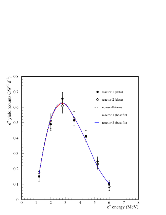
Figure 8: Positron spectra for reactor $1$ and $2$; the solid curves represent the predicted spectra corresponding to the analysis A best-fit parameters, the dashed one to that predicted for no oscillations.

To test a particular oscillation hypothesis $(\delta m^{2},\sin^{2}2\theta)$ against the parameters of the best fit, we adopted the Feldman & Cousins prescription [4]. The exclusion plots at the $90\,\%$ C.L. (solid line) and $95\,\%$ C.L. are shown in Fig. 9.

Figure 9: Exclusion plot for the oscillation parameters based on the absolute comparison of measured vs. expected positron yields.

The region allowed by Kamiokande[5] for the $\nu_{\mu}\rightarrow\nu_{e}$ oscillations is also shown for comparison. The $\delta m^{2}$ limit at full mixing is $7\cdot 10^{-4}\hbox{$\,{\rm eV^{2}}$}$, to be compared with $9.5\cdot 10^{-4}\hbox{$\,{\rm eV^{2}}$}$ previously published[1]. The limit for the mixing angle in the asymptotic range of large mass differences is $\sin^{2}2\theta=0.10$, which is better by a factor of two than the previously published value (as recalculated according to [4]) .

3.2 Results from analysis “B”

The ratio $R(E_{i})\equiv X_{1}(E_{i})/X_{2}(E_{i})$ of the measured positron spectra is compared with its expected values. Since the expected spectra are the same for both reactors in the case of no-oscillations, the expected ratio reduces to the ratio of the average survival probabilities in each energy bin. We can then form the following $\chi^{2}$ function:

$$\chi^{2}=\sum_{i=1}^{7}\big{(}\frac{R(E_{i})-\overline{R}(E_{i},\theta,\delta m^{2})}{\delta R(E_{i})}\big{)}^{2}$$ (14)

where $\delta R(E_{i})$ is the statistical uncertainty on the measured ratio. We adopted the same procedure described in the previous section to determine the confidence domain in the $(\delta m^{2},\sin^{2}2\theta)$ plane. The resulting exclusion plot is shown in Fig. 10; the contour lines of the $90\,\%$ and $95\,\%$ C.L. are drawn.

Figure 10: Exclusion plot contours at $90\,\%$ C.L. and $95\,\%$ C.L. obtained from the ratios of the positron spectra from the two reactors.

Although less powerful than analysis “A”, the region excluded by this oscillation test nevertheless almost completely covers the one allowed by Kamiokande.

3.3 Results from analysis “C”

Analysis “C” is mathematically similar to analysis “A”, the only difference being the omission of the absolute normalization; in “A” we forced the integral counting rate to be distributed around the predicted value ($\alpha=1$), with a $\sigma_{\alpha}=2.7\,\%$ systematic uncertainty; in “C”, $\alpha$ is left free (which is equivalent to $\sigma_{\alpha}=\infty$).

$$\begin{array}[]{ll}\chi^{2}(\theta,\delta m^{2},\alpha,g)~{}=&\\ &\\ \sum_{i=1}^{14}\sum_{j=1}^{14}(X_{i}-\alpha\overline{X}(gE_{i},L_{i},\theta,\delta m^{2}))V_{ij}^{-1}(X_{j}-\alpha\overline{X}(gE_{j},L_{j},\theta,\delta m^{2}))~{}+&\\ &\\ +~{}\big{(}\frac{g-1}{\sigma_{g}}\big{)}^{2}&\end{array}$$

The exclusion plot, obtained according to the Feldman-Cousins prescriptions, is shown in Fig. 11 and compared to the results of analysis “A”.

Figure 11: Exclusion plot at $90\,\%$ C.L. obtained by the shape test (analysis C, solid line) compared to the integral test (analysis A, dashed line).

4 Conclusions

Since publishing its initial findings, the CHOOZ experiment has considerably improved both its statistics and the understanding of systematic effects. As a result it finds, at 90  % C.L., no evidence for neutrino oscillations in the disappearance mode $\overline{\nu}_{e}\rightarrow\overline{\nu}_{x}$ for the parameter region given by approximately $\delta m^{2}>7\cdot 10^{-4}\hbox{$\,{\rm eV^{2}}$}$ for maximum mixing, and ${\rm sin}^{2}2\theta=0.10$ for large $\delta m^{2}$, as shown in Fig. 9. A lower sensitivity result, but independent of most of the systematic effects, is able, alone, to almost completely exclude the Kamiokande allowed oscillation region.

5 Acknowledgements

We wish to thank Prof. Gianni Fiorentini, for initial and fruitful discussions on the two-reactor comparison.
We thank Prof. Erno Pretsch and his group at ETH Zurich, for some precise measurements of the target scintillator hydrogen content.
Construction of the laboratory was funded by Électricité de France (EdF). Other work was supported in part by IN2P3–CNRS (France), INFN (Italy), the United States Department of Energy, and by RFBR (Russia). We are very grateful to the Conseil Général des Ardennes for having provided us with the headquarters building for the experiment. At various stages during construction and running of the experiment, we benefited from the efficient work of personnel from SENA (Société Electronucléaire des Ardennes) and from the EdF Chooz B nuclear plant. Special thanks to the technical staff of our laboratories for their excellent work in designing and building the detector.

References

- [1] M. Apollonio et al., Phys. Lett. B338 (1998) 383.
- [2] K. Schreckenbach et al., Phys. Lett. B160 (1985) 325.
- [3] Y. Declais et al., Phys. Lett. B338 (1994) 383.
- [4] G. J. Feldman & R. D. Cousins, Phys. Rev. D57 (1998) 3873.
- [5] Y. Fukuda et al., Phys. Lett. B335 (1994) 237.