Experimental search for the decay mode $K_{L}\rightarrow\pi^{0}\gamma e^{+}e^{-}$

Abstract

We report on results of a search for the decay mode $K_{L}\rightarrow\pi^{0}\gamma e^{+}e^{-}$ conducted by the E162 experiment at KEK. We observed no events and set a 90% confidence level upper limit of $Br(K_{L}\rightarrow\pi^{0}\gamma e^{+}e^{-})<7.1\times 10^{-7}$ for its branching ratio. This is the first published experimental result on this decay mode.

PACS: 13.20.Eb, 14.40.Aq

, , , , , , , , , , ,

1 Introduction

Chiral perturbation theory ($\chi$PT) is a very powerful tool to describe various $K$ decays in which long distance contributions are expected to dominate. For example, the decay mode $K^{+}\rightarrow\pi^{+}\gamma\gamma$ has been observed recently, and compared with $\chi$PT [1]. The measured branching ratio and $\pi^{+}$ momentum spectrum are found to be consistent with the predictions, after fitting one free parameter contained in the theory. The neutral counterpart, $K_{L}\rightarrow\pi^{0}\gamma\gamma$, is another decay mode, where detailed studies have been performed. In this case, the lowest order $O(p^{4})$ calculation [2] does not reproduce the measured branching ratio [3, 4, 5]. Extending the calculation to the next-to-leading order $O(p^{6})$ [6], and adding a vector meson contribution [7], the prediction is now in good agreement with the branching ratio as well as distinct $M_{\gamma\gamma}$ spectrum. We note that an effective coupling constant ($a_{V}$), a free parameter in the vector meson contribution, has been determined by the measurements with experimental errors [3, 5]. The as yet unobserved decay mode $K_{L}\rightarrow\pi^{0}\gamma e^{+}e^{-}$ can provide another testing ground for $\chi$PT. Since theoretical ingredients are same for both $K_{L}\rightarrow\pi^{0}\gamma\gamma$ and $K_{L}\rightarrow\pi^{0}\gamma e^{+}e^{-}$ modes, a straightforward extension from $K_{L}\rightarrow\pi^{0}\gamma\gamma$ provides definite prediction for a branching ratio and $M_{\gamma ee}$ spectrum [8]. In particular, the branching ratio is calculated to be $2.3\times 10^{-8}$. Thus experimental study of this mode is important to test the theoretical framework of $\chi$PT.

Other interests in this decay mode stem from its close relationship to the mode $K_{L}\rightarrow\pi^{0}e^{+}e^{-}$, which has been of much attention as a possible channel to observe direct $CP$-violation. First, $K_{L}\rightarrow\pi^{0}\gamma e^{+}e^{-}$ is expected to have a much larger branching ratio than $K_{L}\rightarrow\pi^{0}e^{+}e^{-}$, and hence can be an experimental background in a soft photon region. Second, there also exists a $CP$-conserving amplitude in $K_{L}\rightarrow\pi^{0}e^{+}e^{-}$ via two-photon intermediate states; this can be in principle determined from a detail analysis of $K_{L}\rightarrow\pi^{0}\gamma\gamma$ [9]. Further understanding of the $K_{L}\rightarrow\pi^{0}\gamma\gamma$ amplitude, which can be checked by the $K_{L}\rightarrow\pi^{0}\gamma e^{+}e^{-}$ mode, is thus essential.

In this article, we report on an experimental search for the decay mode $K_{L}\rightarrow\pi^{0}\gamma e^{+}e^{-}$ conducted with a proton synchrotron at High Energy Accelerator Research Organization (KEK).

2 Experimental setup

The data for the $K_{L}\rightarrow\pi^{0}\gamma e^{+}e^{-}$ mode were recorded simultaneously with the experiment which has established a new decay mode $K_{L}\rightarrow\pi^{+}\pi^{-}e^{+}e^{-}$ [10]. Since the experimental set-up was described already in Ref. [10, 11], it is briefly mentioned here for convenience.

The $K_{L}$ beam was produced by focusing 12-GeV/c primary protons onto a 60-mm-long copper target. Its divergence was $\pm$4 mrad horizontally and $\pm$20 mrad vertically after a series of collimators embedded in magnets. The set-up started with a 4-m-long decay volume. It was followed by a charged particle spectrometer consisting of four sets of drift chambers and an analyzing magnet with an average horizontal momentum kick of 136 MeV/c. A threshold Cherenkov counter (GC) with pure N₂ gas at 1 atm was placed inside of the magnet gap to identify electrons. For the present decay mode, we obtained an average electron efficiency of 94% with a pion-rejection factor of 350 by adjusting software cuts in the off-line analysis. A pure CsI electromagnetic calorimeter played a crucial role in this analysis. It was located at the downstream end of the spectrometer, and consisted of 540 crystal blocks, each being 70 mm by 70 mm in cross section and 300 mm ($\sim$ 16X₀) in length. It was configured into two banks of 15 (horizontal) $\times$ 18 (vertical) matrix. Its energy and position resolutions were found to be approximately 3% and 7 mm for 1-GeV electrons, respectively. The trigger for the present mode was designed to select events with $\geq$ 2 electron-like tracks and $\geq$ 3 cluster candidates in the calorimeter. It was formed with information from GC and CsI together with trigger scintillator hodoscopes interspersed between the chambers and calorimeter.

3 General event selection

In reconstructing $K_{L}\rightarrow\pi^{0}\gamma e^{+}e^{-}$ events, major backgrounds are expected come from both $K_{L}\rightarrow\pi^{0}\pi^{0}_{D}$ and $K_{L}\rightarrow\pi^{0}\pi^{0}\pi^{0}_{D}$ modes, where $\pi^{0}_{D}$ denotes the Dalitz decay $\pi^{0}\rightarrow e^{+}e^{-}\gamma$. Among them, $K_{L}\rightarrow\pi^{0}\pi^{0}_{D}$ is an intrinsic background and can not be removed. It is instead used as a normalization mode by positively identifying the Dalitz decay. The $K_{L}\rightarrow\pi^{0}\pi^{0}\pi^{0}_{D}$ mode may become background when two (or more) photons fuse into one in the calorimeter, and/or its vertex is reconstructed incorrectly to give false invariant masses. Care was taken in this analysis to enhance position resolution of decay vertex and purity of photon clusters. This effort was found useful also to reject backgrounds originating from external conversions and hadron (mostly neutron) interactions.

In the actual off-line analysis, we first selected events containing two tracks with a common vertex in the beam region inside the decay volume. We then requested events to have $\geq$ 5 clusters in the calorimeter. Here the cluster was defined as $3\times 3$ CsI blocks around the local maximum with the total energy deposit greater than 200 MeV ($\pm$ 3.5 nsec timing window). Particle species were then determined. A charged track which could project onto a CsI cluster was called a matched track. An electron (or positron) was identified as a matched track with 0.9 $\leq$ E/p $\leq$ 1.1, where E was an energy measured by the calorimeter and p was a momentum determined by the spectrometer, respectively. Also GC hits in the corresponding cells were requested. Clusters which did not match with any charged tracks were treated as photon candidates.

Event topology was then checked. We requested events to contain exactly one $e^{+}e^{-}$-pair and three photon candidates, consistent with the $K_{L}\rightarrow\pi^{0}\gamma e^{+}e^{-}$ topology. No additional activities, such as an extra track, GC hit, or cluster with an energy above $\sim$60 MeV, was allowed in the detector. The probability of over-veto was estimated using $K_{L}\rightarrow\pi^{0}\pi^{0}_{D}$ and $K_{L}\rightarrow e^{+}e^{-}\gamma$ reconstructed events, and was found to be about 12% (common to both $K_{L}\rightarrow\pi^{0}\gamma e^{+}e^{-}$ and $K_{L}\rightarrow\pi^{0}\pi^{0}_{D}$ modes).

Two quality cuts were imposed at this stage. One was a cluster shape cut; it examined mainly a cluster’s transverse energy profile, and checked whether or not it was consistent with a single photon. We used a large sample of $K_{L}\rightarrow\pi^{0}\pi^{+}\pi^{-}$ reconstructed events to characterize actual photon showers, and found the cut efficiency to be 95% per a single photon cluster. The other quality cut was imposed on an $e^{+}e^{-}$-track opening angle ($\theta_{ee}$). Larger opening angle resulted generally in better vertex position resolution, which in turn led to better invariant mass resolution and background rejection. We employed a Monte Carlo simulation to study background rejection power, especially for the $K_{L}\rightarrow\pi^{0}\pi^{0}\pi^{0}_{D}$ mode, and determined to demand $\theta_{ee}>$ 20 mrad.

As a final step in the general event selection, we imposed two loose kinematical cuts to reduce sample size. They were $M_{ee\gamma\gamma\gamma}>$ 400 MeV/c² and $\theta^{2}<$ 100 mrad², where $\theta$ represents the angle of the reconstructed $ee\gamma\gamma\gamma$ momentum with respect to the line connecting the target and vertex.

4 Kinematical reconstruction

Having selected candidate events, we scrutinized each event from the viewpoint of kinematical variables. First of all, we calculated $\gamma\gamma$ invariant mass for three possible combinations. The solid-line histogram shown in Fig.1 is the distribution for all combinations while the shaded one for the combination closest to $M_{\pi^{0}}$. We retained all combinations which satisfied $|M_{\gamma\gamma}-M_{\pi^{0}}|<$ 2.5$\sigma_{\pi^{0}}$, where $\sigma_{\pi^{0}}$ being the observed mass resolution of 5.1 MeV/c².

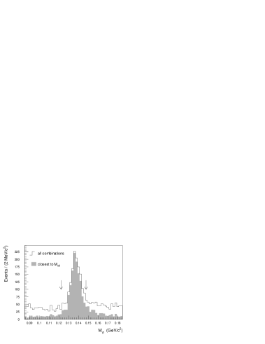
Figure 1: The invariant mass distribution of $\gamma\gamma$. The solid-line histogram shows the distribution for all $\gamma\gamma$ combinations while the shaded one for the combination closest to $M_{\pi^{0}}$. The arrows indicate the cut position.

We then calculated the angle ($\theta^{\ast}$) between reconstructed $\pi^{0}$ and $ee\gamma$ momentum vectors in the $K_{L}$ rest frame. Events originating from $K_{L}\rightarrow\pi^{0}\gamma e^{+}e^{-}$ or $K_{L}\rightarrow\pi^{0}\pi^{0}_{D}$ should satisfy $\cos\theta^{\ast}=-1$ in this frame. The dots with error bars in Fig.2 show the $\cos\theta^{\ast}$ distribution; a clear peak of events at $\cos\theta^{\ast}=-1$ can be seen. The histogram in Fig.2 is Monte Carlo data for the $K_{L}\rightarrow\pi^{0}\pi^{0}\pi^{0}_{D}$ mode, in which the flux was normalized by the observed $K_{L}\rightarrow\pi^{0}\pi^{0}_{D}$ events (see below). To select signals, we requested events to satisfy a collinearity cut, $\cos\theta^{\ast}<-0.98$, as shown by the arrow in Fig.2.

Figure 2: The distribution of $cos\theta^{*}$. The dots with error bars show the experimental data, and the histogram is Monte Carlo data for $K_{L}\rightarrow\pi^{0}\pi^{0}\pi^{0}_{D}$ , in which the flux was normalized by the observed $K_{L}\rightarrow\pi^{0}\pi^{0}_{D}$ events. The cut position ($cos\theta^{*}<$ -0.98) is indicated by the arrow.

We now identify $K_{L}\rightarrow\pi^{0}\pi^{0}_{D}$ events. If more than one $\gamma\gamma$ combination within an event satisfied the $M_{\pi^{0}}$ cut, we selected the one for which the quantity,

$$\chi^{2}_{p}=\left(\frac{M_{ee\gamma}-M_{\pi^{0}}}{\sigma_{\pi^{0}_{D}}}\right)^{2}+\left(\frac{M_{\gamma\gamma}-M_{\pi^{0}}}{\sigma_{\pi^{0}}}\right)^{2},$$

became minimum. Here $\sigma_{\pi^{0}_{D}}$ is the observed $\pi^{0}$ mass resolution for the Dalitz decay mode (see below for the actual value).

Figure 3: (a) The $M_{ee\gamma\gamma\gamma}$ vs $\theta^{2}$ scatter plot of the $K_{L}\rightarrow\pi^{0}\pi^{0}_{D}$ candidate events. (b) The scatter plot of $M_{ee\gamma\gamma\gamma}$ vs $M_{ee\gamma}$ for the events with $\theta^{2}<$ 30 mrad². The box indicates the signal region. (c) The $M_{ee\gamma}$ projection of the events in (b). (d) The $M_{ee\gamma\gamma\gamma}$ projection of the events in (b) with the $\pi^{0}_{D}$ mass cut (see text).

Fig.3(a) shows a scatter plot of $M_{ee\gamma\gamma\gamma}$ vs $\theta^{2}$ after selecting the $\gamma\gamma$ combination with $\chi^{2}_{p}$. To select $K_{L}\rightarrow\pi^{0}\pi^{0}_{D}$ events further, $\theta^{2}<$ 30 mrad² was demanded. Fig.3(b) shows a scatter plot of $M_{ee\gamma\gamma\gamma}$ vs $M_{ee\gamma}$ after this cut. A clear cluster of $K_{L}\rightarrow\pi^{0}\pi^{0}_{D}$ events can be seen in the expected region of $M_{ee\gamma}=M_{\pi^{0}}$ and $M_{ee\gamma\gamma\gamma}=M_{K_{L}}$. Fig.3(c) is the projection onto the $M_{ee\gamma}$ axis, and Fig.3(d) is onto the $M_{ee\gamma\gamma\gamma}$ axis with a $\pi^{0}_{D}$ mass cut (see below). From these projections, we found $\pi^{0}_{D}$ and $K_{L}$ mass resolutions to be $\sigma_{\pi^{0}_{D}}\simeq$ 4.5 MeV/c² and $\sigma_{K_{L}}\simeq$ 16 MeV/c², respectively. Our final signal box, shown by the rectangle in Fig.3(b), was defined by $|M_{ee\gamma}-M_{\pi^{0}}|<~{}$3$\sigma_{\pi^{0}_{D}}$ and $|M_{ee\gamma\gamma\gamma}-M_{K_{L}}|<$ 3$\sigma_{K_{L}}$. After all the cuts, 49 events remained. We estimated the number of $K_{L}\rightarrow\pi^{0}\pi^{0}\pi^{0}_{D}$ backgrounds in the signal region by a Monte Carlo simulation, and found to be less than one.

We are now in a position to look for the $K_{L}\rightarrow\pi^{0}\gamma e^{+}e^{-}$ mode. First we rejected $K_{L}\rightarrow\pi^{0}\pi^{0}_{D}$ events; if an event satisfied both $|M_{\gamma\gamma}-M_{\pi^{0}}|<$ 5$\sigma_{\pi^{0}}$ and $|M_{ee\gamma}-M_{\pi^{0}}|<$ 5$\sigma_{\pi^{0}_{D}}$ for any $\gamma$ combinations, then the event was discarded. Note that we employed the looser kinematical cut of 5$\sigma_{\pi^{0}}$($\sigma_{\pi^{0}_{D}}$) to exclude possible $K_{L}\rightarrow\pi^{0}\pi^{0}_{D}$ events. Then we rejected $K_{L}\rightarrow\pi^{0}\pi^{0}\pi^{0}_{D}$ backgrounds. In this case, an event containing $\pi^{0}_{D}$ whose transverse momentum was consistent with $K_{L}\rightarrow\pi^{0}\pi^{0}\pi^{0}_{D}$ (p${}_{t}<$ 139 MeV/c) was excluded. The remaining events are shown in a scatter plot of $M_{ee\gamma\gamma\gamma}$ vs $\theta^{2}$ in Fig.4(a). We are left with no events inside our signal box defined by $\theta^{2}<$ 30 mrad² and $|M_{ee\gamma\gamma\gamma}-M_{K_{L}}|<$ 3$\sigma^{\ast}_{K_{L}}$. The background events still remaining in the low mass region of $M_{ee\gamma\gamma\gamma}<$ 460 MeV/c² were found to originate mostly from the $K_{L}\rightarrow\pi^{0}\pi^{0}\pi^{0}_{D}$ mode. The projection of events with $\theta^{2}<$ 30 mrad² onto the $M_{ee\gamma\gamma\gamma}$ axis is shown in Fig.4(b). The solid-line histogram is for the data, the shaded one for Monte Carlo events (sum of $K_{L}\rightarrow\pi^{0}\pi^{0}_{D}$ and $K_{L}\rightarrow\pi^{0}\pi^{0}\pi^{0}_{D}$) and the dotted one for $K_{L}\rightarrow\pi^{0}\gamma e^{+}e^{-}$ Monte Carlo events. From the Monte Carlo simulation, whose flux was normalized by the observed $K_{L}\rightarrow\pi^{0}\pi^{0}_{D}$ signals, we expected 1.1 backgrounds (0.45 from $K_{L}\rightarrow\pi^{0}\pi^{0}_{D}$ and 0.66 from $K_{L}\rightarrow\pi^{0}\pi^{0}\pi^{0}_{D}$) to remain in the signal box.

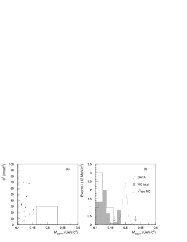
Figure 4: (a) The scatter plot of $M_{ee\gamma\gamma\gamma}$ vs $\theta^{2}$ for $K_{L}\rightarrow\pi^{0}\gamma e^{+}e^{-}$ candidate events. There are no events left inside the signal box. (b) The $M_{ee\gamma\gamma\gamma}$ projection of the events with $\theta^{2}<$ 30 mrad² for the data (solid-line), Monte Carlo (shaded, sum of $K_{L}\rightarrow\pi^{0}\pi^{0}_{D}$ and $K_{L}\rightarrow\pi^{0}\pi^{0}\pi^{0}_{D}$) and $K_{L}\rightarrow\pi^{0}\gamma e^{+}e^{-}$ Monte Carlo (dotted, arbitrary scale). The arrows show the signal region.

5 Results

The branching ratio is calculated by

$$\begin{array}[]{lcl}Br(K_{L}\rightarrow\pi^{0}\gamma e^{+}e^{-})&=&Br(K_{L}\rightarrow\pi^{0}\pi^{0}_{D})\\ &\times&\displaystyle\frac{A(\pi^{0}\pi^{0}_{D})}{A(\pi^{0}\gamma e^{+}e^{-})}\cdot\frac{\eta(\pi^{0}\pi^{0}_{D})}{\eta(\pi^{0}\gamma e^{+}e^{-})}\cdot\frac{N(\pi^{0}\gamma e^{+}e^{-})}{N(\pi^{0}\pi^{0}_{D})},\end{array}$$

where $A$, $\eta$ and $N$ denote acceptance, efficiency and observed number of events, respectively. The detector acceptances depend on the matrix elements: we employed a theoretical model given by Ref. [8] for $K_{L}\rightarrow\pi^{0}\gamma e^{+}e^{-}$ and Kroll-Wada spectrum for the Dalitz decay [12]. The actual acceptances (including the hardware trigger conditions) were determined by Monte Carlo simulations and were found to be $2.34\times 10^{-4}$ for $K_{L}\rightarrow\pi^{0}\gamma e^{+}e^{-}$ and $1.38\times 10^{-4}$ for $K_{L}\rightarrow\pi^{0}\pi^{0}_{D}$, respectively. The detector efficiency was found to be practically same for both modes. However, some of the quality and kinematical cuts caused efficiency differences.

Since the opening angle of $e^{+}e^{-}$-tracks was different for the two modes, it caused efficiency difference in both the vertex reconstruction and the track opening angle cut. These efficiencies were found to be 70% (vertex) and 89% ($\theta_{ee}$) for $K_{L}\rightarrow\pi^{0}\gamma e^{+}e^{-}$ mode while 62% and 81% for $K_{L}\rightarrow\pi^{0}\pi^{0}_{D}$ mode, respectively. Next, the collinearity ($\theta^{\ast}$) cut produced 25% inefficiency for the signal mode while negligibly small loss for the normalization mode. The $\pi^{0}_{D}$ mass cut was unique to $K_{L}\rightarrow\pi^{0}\pi^{0}_{D}$; its efficiency was found to be 96% (3$\sigma$ cut). For the signal mode we rejected $K_{L}\rightarrow\pi^{0}\pi^{0}_{D}$ events; it caused 9% inefficiency at the specific $ee\gamma$ invariant mass region. We also rejected $K_{L}\rightarrow\pi^{0}\pi^{0}\pi^{0}_{D}$ events with the $\pi^{0}_{D}$ inclusive veto; it resulted in 7% inefficiency. Combining other efficiencies together, we found the final acceptance and efficiency ratio $A\eta(\pi^{0}\pi^{0}_{D})/A\eta(\pi^{0}\gamma e^{+}e^{-})$ to be 0.670.

Inserting the known branching ratios [13] into $Br(K_{L}\rightarrow\pi^{0}\pi^{0}_{D})=2\times Br(K_{L}\rightarrow\pi^{0}\pi^{0})\times Br(\pi^{0}\rightarrow\gamma\gamma)\times Br(\pi^{0}\rightarrow e^{+}e^{-}\gamma)$, the single event sensitivity was obtained to be $(3.03\pm 0.43)\times 10^{-7}$, where the error represents the statistical uncertainty. The upper limit on the branching ratio was determined to be

$$Br(K_{L}\rightarrow\pi^{0}\gamma e^{+}e^{-})<7.1\times 10^{-7}\qquad\mbox{(90\% C.L.)},$$

in which the statistical error of the normalization mode was taken into account [14].

In summary, we performed an experimental search for the $K_{L}\rightarrow\pi^{0}\gamma e^{+}e^{-}$ mode. We observed no events and set a 90% confidence level upper limit of $Br(K_{L}\rightarrow\pi^{0}\gamma e^{+}e^{-})<7.1\times 10^{-7}$ for its branching ratio. This is the first published experimental result on this decay mode.

References

• [1] P.Β Kitching et al., Phys. Rev. Lett. 79 4079 (1997).
• [2] G.Β Ecker, A.Β Pich and E.Β de Rafael, Phys. Lett. B 189 363 (1987).
• [3] G.D.Β Barr et al., Phys. Lett. B 242 523 (1990) , B 284 440 (1992).
• [4] V.Β Papadimitriou et al., Phys. Rev. D 44 573 (1991).
• [5] A.Β Alavi-Harati et al., hep-ex/9902029.
• [6] L.Β Cappiello, G.Β D’Ambrosio and M.Β Miragliuolo, Phys. Lett. B 298 423 (1993);
A.G.Β Cohen, G.Β Ecker and A.Β Pich, Phys. Lett. B 304 347 (1993).
• [7] T.Β Morozumi and H.Β Iwasaki, Prog. Theor. Phys. 82 371 (1989);
P.Β Heiliger and L.M.Β Sehgal, Phys. Rev. D 47 4920 (1993);
G.Β D’Ambrosio and J.Β Portoles, Nucl. Phys. B 492 417 (1997).
• [8] J.F.Β Donoghue and F.Β Gabbiani, Phys. Rev. D 56 1605 (1997).
• [9] J.F.Β Donoghue and F.Β Gabbiani, Phys. Rev. D 51 2187 (1995).
• [10] Y.Β Takeuchi et al., Phys. Lett. B 443, 409 (1998).
• [11] T.Β Nomura et al., Phys. Lett. B 408, 445 (1997);
T.Β Nomura, Kyoto University Ph.D thesis (1998) unpublished.
• [12] N.M.Β Kroll and W.Β Wada, Phys. Rev. 98, 1355 (1955).
• [13] Particle Data Group, C.Β Caso et al., Eur. Phys. J. C 3, 1 (1998).
• [14] R.D.Β Cousins and V.L.Β Highland, Nucl. Instrum. Meth. A 320, 331 (1992).