International Journal of Modern Physics A,
c  World Scientific Publishing Company

1

Physics of W bosons at LEP2

Mario Campanelli

Institut für Teilchenphysik

ETH Hönggerberg CH-8093 Zürich

To be published in International Journal of Modern Physics A

After the first observations of W bosons in leptonic interactions, about 4000 WW candidate events per experiment have been collected at LEP2. This data allows the measurement of the WW production cross section at different centre-of-mass energies, as well as W decay branching fractions. The W hadronic branching fraction can be converted into a test of the unitarity of the CKM matrix, or into an indirect determination of the matrix element $|V_{cs}|$. A more direct measurement coming from charm tagging is also performed. The W mass has been measured via the cross section (in the threshold region) and the direct reconstruction of the W decay products, using different techniques to account for the distortions due to experimental effects. The main systematic error to the mass reconstruction in the fully hadronic channel comes from QCD effects like Color reconnections and Bose-Einstein correlations, extensively studied in WW events. In $e^{+}e^{-}$ collisions W pairs can be produced in s-channel via a three vector boson vertex, so a direct study of the trilinear gauge boson couplings is possible. Modification of WW cross section and distributions of W production and decay angles would be an indication of non-standard couplings, thus a first hint for the presence of new physics.

1 Introduction

The experimental program of the LEP accelerator at CERN was foreseen to proceed in two steps: a first period of running around the energy of the Z boson, and a second period at higher energy, having as main goals the production of W boson pairs and the search for new particles.

W bosons can be studied at LEP in a unique environment. Fundamental ingredients of the Standard Model^? as carriers of the charged electroweak interaction, these particles were discovered in 1983 in $p\bar{p}$ collisions by the UA1 and UA2 collaborations at CERN^?,^?,^?. Further, more precise measurements were performed by the CDF and D0 experiments running at the Tevatron collider at Fermilab ^?.

At LEP it is therefore the first time that W bosons are produced in the clean environment of leptonic interactions. In the hadronic case the most copious source of Ws is the Drell-Yan mechanism, with production and subsequent decay of single Ws. Due to the large QCD background to the hadronic decay channel, most of the measurements performed are relative to the cleaner decay channels $W\to e\bar{\nu_{e}}$ and $W\to\mu\bar{\nu_{\mu}}$. In $e^{+}e^{-}$ interactions, W bosons are mainly produced in pairs, and according to their decay WW events can be classified as fully leptonic, semileptonic and fully hadronic. Above the WW production threshold, all decay channels can be studied with small background contamination, giving a broader picture of the physics of these particles.

Measurements of WW and single W production cross sections can be performed, as well as W decay branching ratios, providing a test of lepton universality for charged current interactions.

As it will be discussed in more detail in the next sections, the W mass is one of the fundamental parameters of the Standard Model. Its actual value depends via radiative corrections from unknown parameters like the mass of the Higgs boson, or on the presence of physics beyond the Standard Model. The error on this quantity from the measurements performed at LEP2 is presently the same as that coming from hadronic interactions, and being still dominated by statistics, it will improve in the next years of data taking. Preliminary studies ^? have shown that with the target luminosity of 500 $pb^{-1}$ LEP2 can reach a precision on this quantity $\Delta M_{W}=50$ MeV, with a factor 2 improvement with respect to the present measurements.

The main limitations to the accuracy achievable on the mass are coming from the LEP energy measurement and to final state interactions leading to a distortion of the reconstructed W mass. Since these effect can produce sensible mass shifts, as well as modification in other observables, several models have been proposed and tested with the available data.
The full reconstruction of final states is extremely important for the study of Trilinear Gauge Couplings. S-channel production of W bosons occurs via diagrams involving $\gamma WW$ and $ZWW$ vertices. A deviation from the standard model for these vertices can modify WW production cross section, as well as distributions of W production and decay angles. Constraints on anomalous couplings are coming from the combined studies of WW events, as well as single-W and single-$\gamma$.

If standard model couplings are assumed, W hadronic branching fractions are proportional to squares of CKM matrix elements $|V_{ab}|^{2}$. The matrix element $|V_{cs}|$ is in particular presently known with worse precision with respect to the others; assuming the unitarity of the matrix and the knowledge of the other matrix elements, a more precise determination of this quantity can be derived from the WW hadronic branching fraction. A less precise but more direct determination can be obtained from a charm tagging of the jets from W decays, exploiting heavy-quark characteristics of charm in an environment with small contamination from b quarks.

2 Tree-level relations for gauge bosons

The unified theory of weak and electromagnetic interaction is based on the invariance of the Lagrangian under transformations of the $SU(2)_{L}\times U(1)$ symmetry group. The three fields $(W^{1}_{\mu},W^{2}_{\mu},W^{3}_{\mu})$ are connected to the weak isospin T, and the field $B_{\mu}$ to the weak hypercharge Y. These quantum numbers are related to the electric charge Q by $Q=T_{3}+Y/2$, where $T_{3}$ is the third component of the weak isospin. The physical fields, the carriers of the charged (W^±) and neutral (Z) weak currents, and of the electromagnetic current (A) are linear combinations of the above

$$W^{\pm}_{\mu}=\frac{1}{\sqrt{2}}(W^{1}_{\mu}\mp iW^{2}_{\mu})$$

$$\binom{A_{\mu}}{Z_{\mu}}=\begin{pmatrix}\cos\theta_{W}&\sin\theta_{W}\\ -\sin\theta_{W}&\cos\theta_{W}\end{pmatrix}\binom{B_{\mu}}{W^{0}_{\mu}}$$

The weak angle $\sin\theta_{W}$ introduced relates the coupling constants of the $SU(2)_{L}$ and $U(1)$ interactions to the electric charge

$$g=\frac{e}{\sin\theta_{W}}$$

$$g^{\prime}=\frac{e}{\cos\theta_{W}}$$

At low energies, the electroweak theory is equivalent to the Fermi theory of the weak interactions. The Fermi constant can be expressed as

$$G_{F}=\frac{g^{2}}{4\sqrt{2}M_{W}^{2}}=\frac{\pi\alpha_{QED}}{\sqrt{2}M_{W}^{2}\sin^{2}\theta_{W}}$$

Since vector bosons behave as real particles, a gauge-invariant kinetic term must be added to the Lagrangian describing electroweak interactions. Due to the non-Abelian structure of the gauge field, the commutators of the covariant derivatives involved do not vanish, but produce terms leading to the self-interaction of the gauge bosons:

$${\cal L}_{W}^{kin}=-\frac{1}{4}W^{j}_{\mu\nu}W_{j}^{\mu\nu}$$

$$W^{j}_{\mu\nu}=\partial_{\mu}W^{j}_{\nu}-\partial_{\nu}W^{j}_{\mu}+g\epsilon^{j}_{km}W^{k}_{\mu}W^{m}_{\nu}$$

The last term involves the product of two W fields, so in the Lagrangian terms for trilinear and quadrilinear gauge boson interactions are present.

In the standard model the vector bosons acquire a mass by the spontaneous breaking of the symmetry group, introducing a Higgs ^? doublet

$$\binom{\Phi^{+}}{\Phi^{0}}=\binom{\Phi_{1}+i\Phi_{2}}{\Phi_{3}+i\Phi_{4}}$$

and choosing a vacuum expectation value $|\Phi^{0}|^{2}=v^{2}/2>0$. The masses of the vector bosons are then determined by this vacuum expectation value and the coupling constants:

$$m_{W}=\frac{gv}{2},\hskip 56.9055ptm_{Z}=\frac{\sqrt{g^{2}+{g^{\prime}}^{2}}}{2}v,\hskip 56.9055ptm_{\gamma}=0$$

which leads to a relation between the masses of the vector bosons and the weak angle

$$\cos^{2}\theta_{W}=\frac{m^{2}_{W}}{\rho m^{2}_{Z}}$$

The $\rho$ parameter is equal to unity at tree level. Deviations from this value can arise from radiative corrections.

3 Indirect determination of the W mass

To obtain accurate predictions, the tree-level relations presented above are no longer sufficient, but the evaluation of higher orders is needed, especially given the accuracy of the available data. An example is the possibility of extracting the W mass from the standard model relations without directly measuring this quantity. From the equations shown in the previous section, it is possible to derive

$$\sqrt{2}G_{F}M^{2}_{W}(1-\frac{M^{2}_{W}}{\rho M^{2}_{Z}})=\pi\alpha$$

To include higher-order effects, different schemes can be used. The most common approach ^? is to keep $\rho$ to its tree level value 1 and include all corrections in a quantity $\Delta r$, that accounts for both weak and electromagnetic effects:

$$\sqrt{2}G_{F}M^{2}_{W}(1-\frac{M^{2}_{W}}{M^{2}_{Z}})=\frac{\pi\alpha}{1-\Delta r}$$

Since $\alpha$, $G_{F}$ and $M_{Z}$ are experimentally well known quantities, it is possible to derive the W mass from

$$M_{W}^{2}=\frac{1}{2}M_{Z}^{2}(1+\sqrt{1-\frac{4A_{0}^{2}}{M_{Z}^{2}}\frac{1}{1-\Delta r}})$$

with

$$A_{0}^{2}=\frac{\pi\alpha}{\sqrt{2}G_{F}}$$

In the standard model, vertex and propagator corrections can be decoupled into an electromagnetic part, due to the running of the coupling constant $\alpha_{QED}$, and a weak part, that contains terms showing a quadratic dependence on the top mass and a logarithmic dependence on the Higgs mass:

$$\Delta r=\Delta\alpha+\frac{\cos^{2}\theta_{W}}{\sin^{2}\theta_{W}}\frac{3G_{\mu}m_{t}^{2}}{8\pi^{2}\sqrt{2}}+\frac{\sqrt{2}G_{\mu}M_{W}^{2}}{16\pi^{2}}[\frac{11}{3}(\log\frac{m_{H}^{2}}{M_{W}^{2}}-\frac{5}{6})]+...$$

The mass of those particles enters therefore as a parameter to the indirect determination of the W mass, as can be seen in figure 1 (full curve), where a clear correlation emerges between the indirect determinations of the masses of the W and the top quark, as extracted from a fit to precision electroweak data (mainly coming from LEP1 measurements) available in winter 1999 ^?.

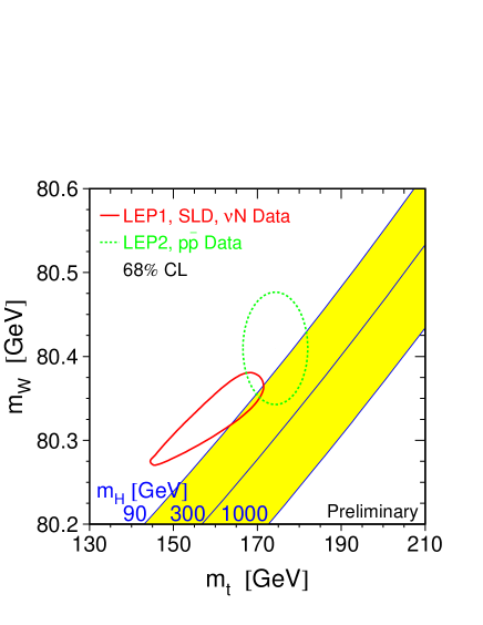
Figure 1: Comparison between the direct measurements of the masses of W and top mass and the predictions from the electroweak fit, for various values of the Higgs mass

The plot also shows as a dotted ellipse the direct measurement of both masses, in good agreement with the indirect predictions. It is possible then to also include the measured value of $m_{t}$ and $m_{W}$ in the fit, and get some indication on the mass of the Higgs boson.

It is therefore very important to improve the precision on the direct determination of the W mass, to further constraint the standard model, and get stronger bounds on the allowed range for the Higgs mass.

4 Models for Trilinear Gauge Coupling

We have already seen that in the standard model vertices involving gauge bosons only derive from the request of gauge invariance of the kinetic term. Since trilinear couplings are extensively studied at LEP2, possible deviations from the standard model value will be discussed.

The most general Lorenz-invariant effective Lagrangian, expressing the coupling of two oppositely charged and one neutral vector bosons is the following^?:

$${\cal L}_{WWV}^{eff}/g_{WWV}=ig_{1}^{V}(W_{\mu\nu}^{\dagger}W^{\mu}V^{\nu}-W_{\mu}^{\dagger}V_{\nu}W^{\mu\nu})+ik_{V}W_{\mu}^{\dagger}W_{\nu}V^{\mu\nu}$$

$$+\frac{i\lambda_{V}}{m_{W}^{2}}W_{\mu\nu}^{\dagger}W^{\mu}_{\rho}V^{\nu\rho}-g_{4}^{V}W_{\mu}^{\dagger}W_{\nu}(\partial^{\mu}V^{\nu}+\partial^{\nu}V^{\mu})$$

$$+g_{5}^{V}\epsilon^{\mu\nu\rho\sigma}(W^{\dagger}_{\mu}\overrightarrow{\partial_{\rho}}W_{\nu})V_{\sigma}+i\tilde{k}_{V}W_{\mu}^{\dagger}W_{\nu}\tilde{V}^{\mu\nu}$$

$$+\frac{i\tilde{\lambda}_{V}}{m_{W}^{2}}W_{\mu\nu}^{\dagger}W_{\rho}^{\mu}\tilde{V}^{\nu\rho}$$

Here V stands for either a photon or a Z boson ($V=\gamma,Z$), and W for the W field. $g_{WWV}$ are fixed to

$$g_{WW\gamma}=-e\hskip 85.35826ptg_{WWZ}=-e\cot\theta_{W}.$$

At tree level, the SM predicts $g_{1}^{Z}=g_{1}^{\gamma}=k_{Z}=k_{\gamma}=1$, with all other couplings vanishing. The terms $g_{1}^{V},k_{V}$ and $\lambda_{V}$ conserve C and P separately, while $g_{5}^{V}$ violates both C and P conserving CP. The coupling between W and photons can be related to intuitive physical quantities; in particular the terms conserving C and P correspond to the lowest-order terms in a multipole expansion of the interactions between Ws and photons; thus they can be related to the magnetic moment $\mu_{W}$ and the electric quadrupole moment $Q_{W}$:

$$\mu_{W}=\frac{e}{2m_{W}}(1+k_{\gamma}+\lambda_{\gamma})$$

$$Q_{W}=-\frac{e}{m_{W}^{2}}(k_{\gamma}-\lambda_{\gamma})$$

The two parity-violating couplings $\tilde{k}_{\gamma}$ and $\tilde{\lambda}_{\gamma}$ respect charge-conjugation invariance, and are related to the electric dipole moment $d_{W}$ and to the magnetic quadrupole moment $\tilde{Q}_{W}$:

$$d_{W}=\frac{e}{2m_{W}}(\tilde{k}_{\gamma}+\tilde{\lambda}_{\gamma})$$

$$\tilde{Q}_{W}=-\frac{e}{m_{W}^{2}}(\tilde{k}_{\gamma}-\tilde{\lambda}_{\gamma}).$$

Due to the relatively limited statistics available in the present experimental facilities, the set of free parameters present in the general Lagrangian quoted above is too large for practical uses. This set of parameters can be reduced under a certain number of assumptions, depending on the way the effective Lagrangian quoted above is made gauge-invariant, i.e. what kind of new physics is expected to generate the couplings. If a light Higgs boson is present, and considering only the C- and P- conserving operators, the effective Lagrangian can take the gauge-invariant form

$${\cal L}^{TGC}=ig^{\prime}\frac{\alpha_{B\Phi}}{m_{W}^{2}}(D_{\mu}\Phi)^{\dagger}B^{\mu\nu}(D_{\nu}\Phi)+ig\frac{\alpha_{W\Phi}}{m_{W}^{2}}(D_{\mu}\Phi)^{\dagger}\tau W^{\mu\nu}(D-\nu\Phi)+g\frac{\alpha_{W}}{6m_{W}^{2}}W^{\mu}_{\nu}(W^{\nu}_{\rho}\times W^{\rho}_{\mu})$$

with g and g’ the SM couplings of the $SU(2)_{L}$ and $U(1)_{Y}$ symmetries. When the Higgs field is replaced by its vacuum expectation value $(0,v/\sqrt{2})$, the following relations can be written:

$$\Delta g^{Z}_{1}=g^{Z}-1=\frac{\alpha_{W\Phi}}{\cos^{2}\theta_{W}}$$

$$\Delta k_{\gamma}=(k_{\gamma}-1)=-\frac{\cos^{2}\theta_{W}}{\sin^{2}\theta_{W}}(\Delta k_{Z}-\Delta g_{1}^{Z})=\alpha_{W\Phi}+\alpha_{B\Phi}$$

$$\lambda_{\gamma}=\lambda_{Z}=\alpha_{W}$$

and is then natural to use the above relations and express all measured quantities as a function of $(\Delta g_{1}^{Z},\Delta k_{\gamma},\lambda_{\gamma})$ or the $\alpha$ parameters.

In the absence of a light Higgs, a non linear approach can be followed to make the effective Lagrangian gauge-invariant. In this scheme, it is convenient to express the couplings as a function of the lowest-dimension operators $(\Delta g_{1}^{Z},\Delta k_{\gamma},\Delta k_{Z})$, while the parameters $\lambda_{\gamma}$ and $\lambda_{Z}$ are usually set to zero.

5 Four-fermion production in $e^{+}e^{-}$ collisions

Processes involving W pair production in e⁺e^- collisions are a subset of a larger set of diagrams contributing to four-fermion final state and interfering with each other, so all of them have to be considered when dealing with W events. Processes contributing to 4-fermion final states can be divided into charged current (CC) and neutral current (NC). The first class comprises production of (up, antidown) and (down-antiup)-type fermion pairs, where each pair has the same generation index. Final states produced via W production belong to this class. Neutral current events are those where two fermion-antifermion pairs are produced, and they are mediated by the neutral gauge bosons. Obviously these two classes overlap for certain final states. The number of Feynman diagrams contributing to the charged current class is shown in table 1 for the possible combinations of final states. Three different cases occur (shown in the table by different character types):

• CC11 family (boldface): for two different fermion pairs, none of which is an electron, or electron neutrino, no identical particles are involved, and there is at maximum 11 diagrams.

• CC20 family (normal): one e^± and one $\nu_{e}$ are in the final state, so additional diagrams with t-channel exchange of the gauge boson are present

• CC43/mix43 CC56/mix56 (italics): two mutually charge conjugate pairs are produced, so these diagrams can proceed via both charged and neutral gauge boson exchange

	$\bar{d}u$	$\bar{s}c$	$\bar{e}\nu_{e}$	$\bar{\mu}\nu_{\mu}$	$\bar{\tau}\nu_{\tau}$
$d\bar{u}$	43	11	20	10	10
$e\bar{\nu_{e}}$	20	20	56	18	18
$\mu\bar{\nu_{\mu}}$	10	10	18	19	9

Table 1: Number of diagrams for Charged Current final states

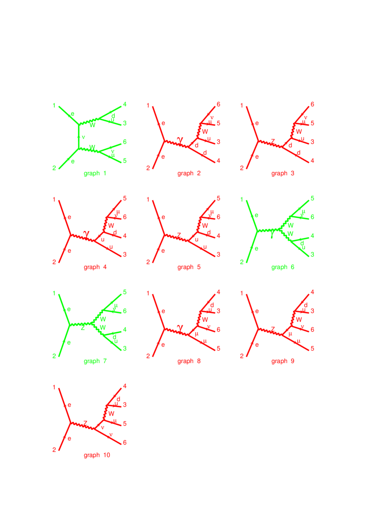
Figure 2: Feynman diagrams involved in $e^{+}e^{-}\to u\bar{d}\mu\bar{\nu_{\mu}}$ final state. Graphs in light grey (1, 6 and 7) correspond to W pair production (CC03)

In figure 2 the 10 diagrams contributing at tree level to the e⁺e${}^{-}\to u\bar{d}\mu\bar{\nu_{\mu}}$ events are shown. All semileptonic decays (except those where an electron is present in the final state) are produced through the same set of diagrams, with the proper redefinition of the final state particles. The graphs 1, 6 and 7 are the only ones where a W pair is produced; they are often referred to as CC03 processes. Contributions from single- and non-resonant processes are particularly large for $l\nu l\nu$ and $qqe\nu$ final states, leading to an ambiguity in the definition of the signal. The approach followed by the LEP collaborations is slightly different:

• DELPHI, L3: consider efficiencies on signal inside generator level cuts, and apply multiplicative factors for translating the cross section measured for the full set of diagrams into a cross section relative to W-pair production only

• ALEPH, OPAL: consider the additional diagrams as a background, neglecting the interference between these processes and the W pair diagrams

It was shown that these procedures give the same results within a 1% accuracy.

6 Machine parameters, schedule and calibration

Due to the strong increase in synchrotron radiation, the only possibility to operate the LEP machine well above the Z resonance is to considerably increase the LEP1 accelerating power. Since the machine layout cannot be changed, this can only be achieved raising the accelerating gradient in the straight sections. The 128 five-cell copper cavities constituting the accelerating system of LEP in the first phase were able to deliver a peak RF power corresponding to a voltage of 400 MV per revolution, clearly inadequate for LEP2 needs (over 3000 MV). The big increase in performances was only possible due to the operation of superconducting cavities, that because of their very high quality factor could provide as much as 6 MV/m of accelerating gradient.

The installation of those cavities proceeded in several steps, and so did the energy of operation of the machine. The machine schedule in the period 1996-1997 is shown in table 2, where only the data-taking periods with total energy above the Z peak have been considered. Apart from the runs above the WW threshold, relevant to this report, a short run at 130-136 GeV has been taken, to clarify possible anomalies in the 4-jet production at that energy. The results of that run are summarized in ^?.

Period	N. SC cavities	N. Cu cavities	$\int{\cal L}$ (pb-1)	Energy (GeV)
1996 a	144	182	12.1	161
1996 b	176	150	11.3	172
1997	240	86	63.8	183
1997 b	240	86	7.2	130-136
1998	272	48	196.4	189

Table 2: Characteristics and performances of the LEP machine in the years 1996-1998. Only runs above the Z peak have been listed.

Since all fitting methods use the centre-of-mass energy as a kinematic constraint, the uncertainty on the knowledge of the LEP beam energy directly reflects into a systematic error on the value of the W mass:

$$\Delta M_{W}=\frac{\Delta E_{b}}{E_{b}}M_{W}$$

To fulfill the requested precision on the mass, the LEP energy has to be known with an accuracy better than 20 MeV. At LEP1, energy calibration was performed via resonant depolarization (RDP)^?. This method can not be used at LEP2, since there is no possibility to have polarization at physics energies. Several RDP measurements have been however performed at lower energies, and extrapolated. The main error on this method comes from the extrapolation itself, leading to a total error of about 20 MeV at 189 GeV.

As an independent approach, a spectrometer is planned for LEP, to be operational in 1999 and beyond. This will consist in a fully equipped dipole magnet, giving a precision of about $1\mu m$ on the beam position, extracting the particle momentum out of their curvature in the dipole magnetic field.

7 WW cross section and branching ratios

WW events can have very different topologies, depending on the different decays of the two W bosons. As two extreme cases, the decay of two W bosons could produce a high-multiplicity four-jet event, as well as a low-energy imbalanced event with only two charged leptons seen in the detector.

Accordingly, the selection criteria, the backgrounds and the possible systematic uncertainties in the selections can be very different. All LEP collaborations have different analysis for the possible WW decay channels. They are here grouped into three main categories: fully leptonic, semileptonic and fully hadronic decays.

7.1 Fully leptonic events

Fully leptonic events $WW\to l\nu l\nu$ are usually characterized by:

• two high-energy acoplanar leptons

• missing momentum not pointing to the beam pipe, due to the undetected neutrinos

An example of a $l\nu l\nu$ event detected in the DELPHI detector is shown in figure 4. The energy distribution of the most energetic lepton in L3 for $l\nu l\nu$ candidates is in figure 4.

Events are usually classified into lepton-lepton, lepton-jet and jet-jet categories, where here lepton stands for either electron or muon, and narrow jets are considered, to account for hadronic $\tau$ decays.

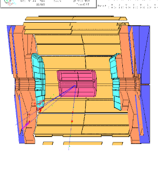
Figure 3: A $WW\to\tau\nu\mu\nu$ event in Delphi. A narrow jet originated from $\tau$ decay (on the left), and a muon (traversing the whole detector) are widely acoplanar.

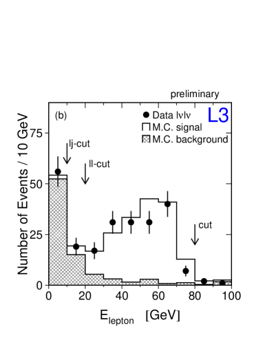
Figure 4: Lepton energy distribution in L3 for fully leptonic events

Due their topology, the main backgrounds to these processes are:

• Two-fermion events from $Z/\gamma$ decays (especially $\tau$ pair production), Bhabha scattering events

• high-energy $\gamma-\gamma$ interactions

• $ZZ\to ll\nu\nu$ events (mainly for $\sqrt{s}>184$ GeV)

Since the leptons are required to be acoplanar, the most dangerous background from two fermion events is represented by radiative $Z/\gamma$ decays. Events with a high-energy isolated photon are rejected, since this is a clear indication of radiative $Z/\gamma$ decays. Also events with missing momentum pointing at very low angle are rejected, since in this case the radiated photon could have been lost in the beam pipe or in a badly-instrumented sector of the detector. The typical selection efficiencies for this channel are higher for the case in which two stable leptons are produced, and lower for the jet-jet case, due to the stronger cuts needed to suppress the larger background. Overall efficiencies are around 70%.

7.2 Semileptonic events

The semileptonic channels $WW\to q\bar{q}l\bar{\nu}_{l}$, in particular those with an electron or a muon in the final state, have quite similar topology. These events are characterized by two hadronic jets, a high-energy lepton and large (and similar) missing energy and momentum due to the neutrino. $qq\tau\nu$ events are usually more balanced due to the additional neutrinos produced in $\tau$ decays, and the missing energy is larger. The lepton from $\tau\to e$ and $\tau\to\mu$ decays is softer, than that produced directly from the W, while hadronic $\tau$ decays produce a narrow jet.

The background is mainly coming from hadronic Z radiative decays, but is different for the three channels. For the $qqe\nu$ case, the main baground comes from Z radiative events with the photon in the detector, associated to a nearby track, or converted into a $e^{+}e^{-}$ pair. This is particularly true in the forward region of the detector, where most of the radiative photons are emitted, and where usually the tracking capabilities of the detector are not optimal. Background to the $qq\mu\nu$ channel is mainly coming from semileptonic decays of b quarks in $Z\to qq(\gamma)$ events, or from $ZZ\to qq\mu\mu$ processes, where one of the muons is not identified, and mimics missing momentum. Having less strong signature, the $qq\tau\nu$ channel has usually more complicated selections, and its main background arises from radiative Z hadronic decays where the photon gets undetected and a third jet fakes that coming from $\tau$ decays.

For the final selection, DELPHI and L3 use a cut-based approach, requiring good isolation for the lepton and high invariant mass for the decay products of the two Ws. ALEPH and OPAL combine the informations coming from similar variables using an event probability function. Typical efficiencies are of the order of 80% for the electron and muon channels, and 50% for the $\tau$ channel.

Figure 5: A $qqe\nu$ event in L3. The electron is visible as a large “tower” in the electromagnetic calorimeter, in the bottom part of the event. The two hadronic jets are opposite to each other.

Figure 6: Distributions of measured lepton energies for events selected in OPAL in the three semileptonic channels

7.3 Hadronic W decays

The channel $WW\to q\bar{q}q\bar{q}$ has about the same branching ratio as the sum of three semileptonic ones, i.e. about half of the total number of WW decays. It is characterized by four high-energy well separated hadronic jets, coming from hadronization of the quarks from the W decays.

There are two main sources of background:

• $Z\to q\bar{q}$ events with hard gluon radiation

• $ZZ\to q\bar{q}q\bar{q}$ events.

The latter is almost irreducible, since well-isolated high energy jets are produced, and the only difference with respect to the signal is the slightly higher jet-jet invariant mass. Z decays have a larger cross section, but since the two additional jets are coming from gluon radiation, they are usually less energetic and closer to the emitting quark.

All experiment try to combine all available informations in an optimized way. This is done combining several variables (event shape, invariant masses angles between jets etc.), using a likelihood discriminator (OPAL) or a neural network (DELPHI,ALEPH, L3). The variables used by the OPAL collaboration are shown in figure 7, together with the resulting likelihood and the value of the cut. In order to have an additional gain in statistical power and have a further cross-check on the background, ALEPH and L3 fit the neural network output distribution by a linear combination of distributions for signal and background.

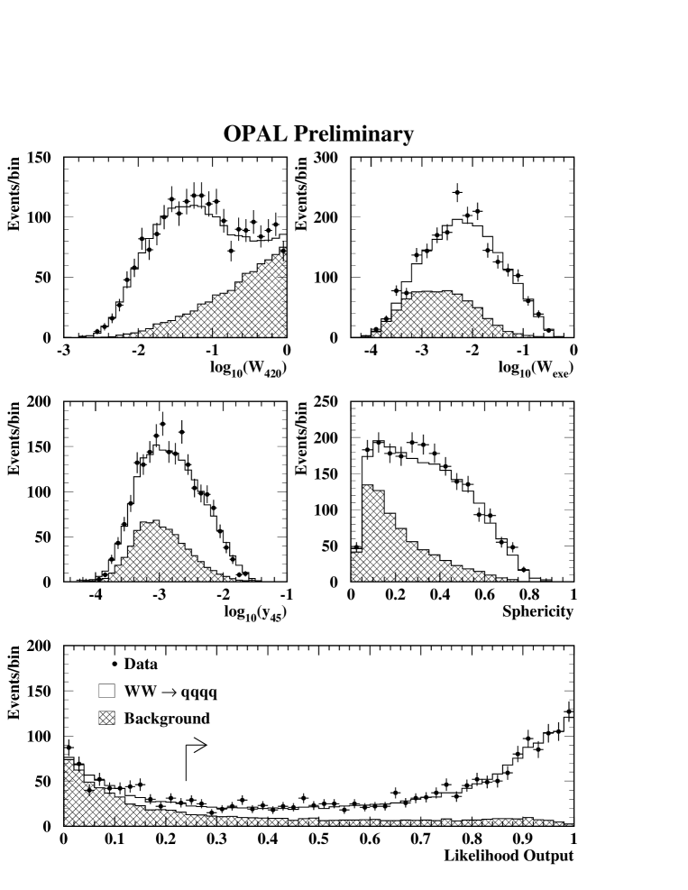
Figure 7: Distributions of the variables used by OPAL in the $WW\to q\bar{q}q\bar{q}$ analysis. The points indicate the data, the open histogram represents the MonteCarlo expectations for the signal, and the hatched histogram shows the background estimate.

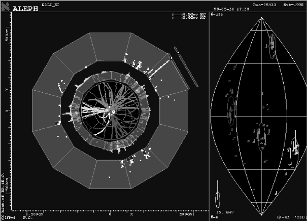
Figure 8: A $WW\to q\bar{q}q\bar{q}$ event in ALEPH. The four jets coming from W decays are clearly separated.

The uncertainties related to the QCD modeling of the fragmentation process, in particular of the final state interactions, are the main sources of systematic errors for this channel. These uncertainties will be discussed in more detail in the section about W mass measurements.

8 Determination of WW cross section and branching fractions

The cross sections for the individual WW decay channels measured as above are combined to extract a value of the total WW production cross section and branching ratio. To make use of physical assumption like i.e. lepton universality, likelihood-based fit are used by the different collaborations. For a given channel $i$, the expected number of events, $\mu_{i}$, is computed accounting for the background and the cross-efficiencies among that channel and all the others ($\epsilon_{ij}$):

$$\mu_{i}=L\times(\Sigma_{j}\epsilon_{ij}\sigma_{j}+\sigma_{i}^{bg})$$

where L is the collected luminosity and the sum runs on all channels. The cross sections are extracted maximizing the likelihood

$${\cal L}=\Pi_{i}P(N_{i},\mu_{i})$$

where P is the Poisson probability of observing $N_{i}$ events in a given channel i, with $\mu_{i}$ expected.

This likelihood can be maximized leaving different free parameters, according to the physics assumptions. If for instance no assumptions are made, the cross sections $\sigma_{j}$ for all channels are left free. On the other hand, it is possible to extract the total cross section, imposing the knowledge of the W standard model branching fractions. In this case, the above cross sections are expressed as the product of the WW cross section $\sigma$ (which is now the only free parameter in the fit) times the branching ratio for the corresponding channel.

The total WW production cross section for the four experiments at $\sqrt{s}$ of 183 and 189 GeV are listed in table 8. All results from the run at 189 GeV are preliminary, and taken from the contributions of the various collaborations to the winter conferences^?.

Cross-section $\sigma_{\tt CC03}$ (pb)
Experiment	$\sqrt{s}=$183 GeV	$\sqrt{s}=$189 GeV
ALEPH	15.57 $\pm$ 0.68n	15.64 $\pm$ 0.43
DELPHI	15.86 $\pm$ 0.74n	15.79 $\pm$ 0.49
L3	16.53 $\pm$ 0.72p	16.20 $\pm$ 0.46
OPAL	15.43 $\pm$ 0.66p	16.55 $\pm$ 0.40
LEP	15.83 $\pm$ 0.36	16.07 $\pm$ 0.23
SM	15.70 $\pm$ 0.31	16.65 $\pm$ 0.33
p Published n New Preliminary

The combined LEP cross section only considers statistical errors. The combined value for all LEP2 energies is shown in figure 9. In addition to the curve predicted from the standard model, this figure shows the WW cross section in the two cases where the ZWW vertex has zero coupling, and where WW production occurs only via the neutrino exchange diagram. In both cases the WW production cross section diverges for large values of $\sqrt{s}$, and is also incompatible with the values measured at LEP. Therefore, the simple cross section measurement represents a confirmation of the non-Abelian structure of the electroweak interactions.

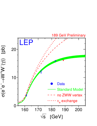
Figure 9: Total WW production cross section

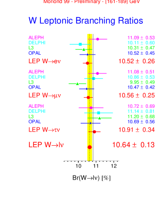
Figure 10: Leptonic branching ratios

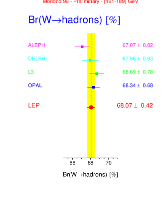
Figure 11: Hadronic branching ratios

If the cross section is not fixed, it is possible to determine the W decay branching ratios, leaving them as free parameters for the fit. The results for the different leptonic ratios is shown in figure 11, showing a direct verification of th lepton universality in charged current weak interactions. The hadronic branching ratio is shown in figure 11. This value can be expressed in terms of the CKM matrix elements using the following expression:

$$\frac{Br(W\to q\bar{q})}{1-Br(W\to q\bar{q})}=(1+\frac{\alpha}{\pi})\Sigma|V_{ij}|^{2}$$

that yields, using the combined LEP value:

$$\Sigma|V_{ij}|^{2}=2.10\pm 0.08$$

The experimental knowledge of all elements of the CKM matrix is quite good, apart from $V_{cs}$, suffering from large uncertainties (about 20%) of both experimental and theoretical nature^?. Imposing unitarity of the CKM matrix and considering the measurements of the other matrix elements, the previous result can be reinterpreted as a determination of $|V_{cs}|$:

$$|V_{cs}|=1.002\pm 0.0016(stat)\pm 0.002(syst)$$

A completely independent technique to determine this quantity will be presented in section 12.

9 W mass

As mentioned in the introduction, the W mass is one of the most important measurements of the LEP2 program. At energies close to the WW production threshold, the highest sensitivity is reached deriving the mass from the cross section measurement, an approach conceptually similar to that used at LEP1 to measure the mass of the Z boson. At higher energies, the W mass is derived directly from the measured invariant mass of the W decay products.

9.1 W mass from threshold cross section

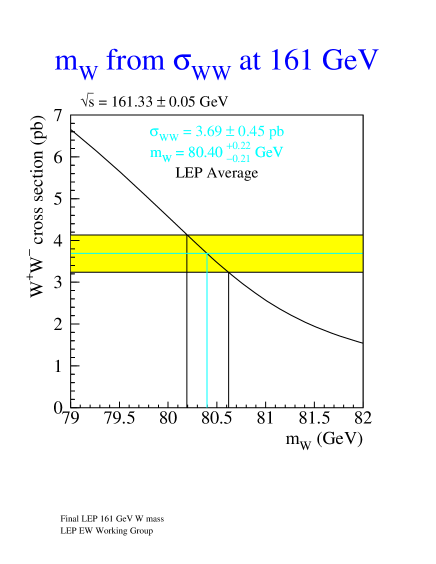
Figure 12: W mass from the combined LEP cross section at $\sqrt{s}=161$ GeV

Assuming validity of the SM, the W mass can be extracted from the cross section, for a fixed centre-of-mass energy. The sensitivity of this approach is maximal close to threshold, due to the steep rising of the cross section in that region; for this reason this method was used to determine the mass from the cross section of the first run at $\sqrt{s}=161$ GeV. In figure 12 the dependence of the cross section on the W mass is shown, together with the combined measurement of the mass from the LEP experiments.

9.2 W mass from direct reconstruction

At higher energies the dependence of the cross section on the W mass is negligible, so the derivation of the mass from the cross section can no longer be used. On the other hand, the WW cross section is much larger than at threshold, and it is possible to use the direct reconstruction method, i.e. the W mass is extracted with a fit to the invariant mass distribution of the W decay products. The calculation of these masses is only trivial in the semileptonic case, where two jets are coming from a W and the system of lepton and neutrino from the other. In the fully leptonic case, the system is underconstrained, due to the presence of at least two undetected neutrinos. The ALEPH collaboration has been the only one so far to use this channel for mass fits, using the energy of the two leptons, with small statistical power. In the fully hadronic case, since at least four jets are present in the detector, several mass pairs could be formed. Criteria based on reconstructed masses, angles etc. are used to get the best pairing, with efficiencies of the order of 80%; however including the other pairings with smaller weight can help increasing the mass sensitivity.

The main problem to measure the W mass from reconstructed distribution is to account for all distortions coming from detector effects and selection biases. Two main approaches are used:

• convolution

• MC reweighting

All LEP collaborations use both methods, quoting one for the final results and the other as a cross-check.

In both cases the final error on the W mass will be determined by the total number of candidates as well as the detector resolution in measuring invariant masses. In order to improve the detector performances, it is possible to impose some physical constraint to any single event. Since energy and momentum are conserved in the collision, it is possible to perform a fit to energies and angles of the final states particles, such that the fit results satisfy the kinematical constraint and are as close as possible to the measured ones. This procedure largely increases the sensitivity to the W mass, but requires a precise knowledge of the LEP energy since this value is directly used in imposing the energy conservation.

The L3 and OPAL collaboration also exploit the additional kinematical constraint that the masses of the two produced W bosons must be equal within the W width.

9.3 Convolution

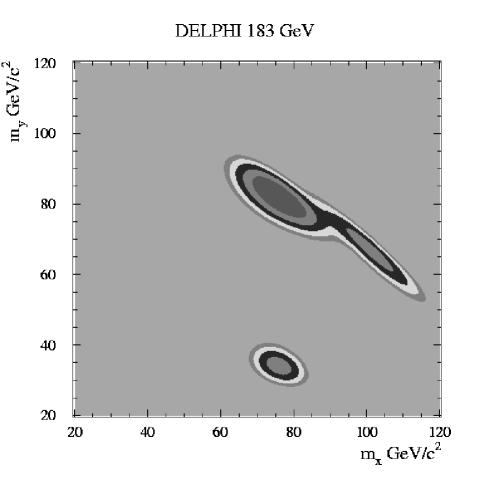
Figure 13: Likelihood contours in the $M^{1}_{W}-M^{2}_{W}$ plane for a four-jet event in DELPHI. The three maxima correspond to the three possible jet pairings.

In the convolution method (DELPHI), the theoretical W line-shape curve (depending on the W mass) is convoluted with an analytical function describing detector effects. The experimental line-shape is compared to the convoluted curve, determining a likelihood function, having as a free parameter the W mass. Maximizing the likelihood it is possible to extract the value of the W mass for which the curve obtained smearing the theoretical distribution mostly resembles the experimental curve.

The main difficulty of this method is in the modelization of the the detector response, that must be included an analytical form. Morover, the reconstructed mass has a bias that must be corrected comparing with the MC. On the other hand, the method allows the use of different event weights depending on the detector resolution for each data event, thus improving the accuracy of the measurement.

In particular, DELPHI fits the masses in the $M_{W}^{1}$, $M_{W}^{2}$ plane, using all three combinations for the qqqq channel (see figure 13).

9.4 MC Reweighting

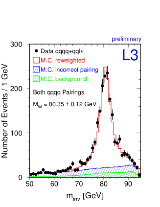
Figure 14: W mass distribution in L3

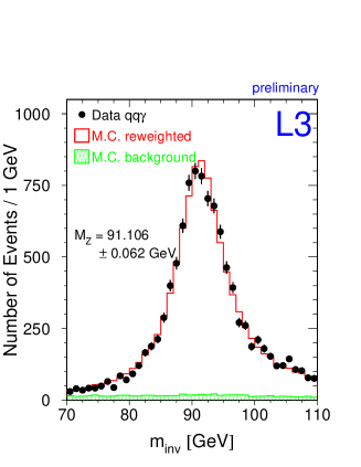
Figure 15: Z mass distribution in L3

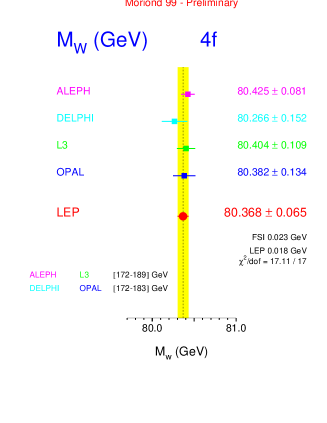
Figure 16: Results for the W mass from direct reconstruction in the four LEP experiments. ALEPH-L3: preliminary results including the run at 189 GeV; OPAL-DELPHI: final results from the runs at 172 and 183 GeV of centre of mass energy

This method, used by the other collaborations, uses a large number of Monte Carlo events to establish the correspondence between generated and reconstructed masses. These events are generated with a given value of the W mass; an analytical code is used to reweight them according to the mass that best fits the data, using an iterative procedure based on a likelihood similar to that used for the convolution method.

As a cross-check for the validity of the method, the L3 collaboration has presented a fit to the Z mass, performed on radiative $Z\to q\bar{q}\gamma$ events, using the same method as the one used to fit the mass of the W. Since the value of the Z mass is known with very high precision from LEP1 measurements, the good agreement of the fitted value with the expectation is a good test of the complete mass analysis method. In figures 15 and 15, the reconstructed invariant mass distributions for WW (all channels) and radiative Z events are shown. It is interesting to notice that for hadronic WW events the two best jet pairing are included, so a large but flat background from incorrect jet pairing is present.

Both method can be used to perform a two-parameter fit, where both $M_{W}$ and $\Gamma_{W}$ are left free. The correlation of the two measurements is quite small, and a statistical error of about 200 MeV per experiment on the width measurement can be obtained.

The W mass results from direct reconstruction are shown in figure 16. In this plot, all results refere to data taken at center of mass energies between 172 and 189 GeV^?.

The present combined value from LEP is $M_{W}=80.368\pm 0.065$ GeV (statistical error only), as precise as the combined value obtained from hadron machines.

9.5 Systematic uncertainties on the mass measurement

Given the importance of the measurement of the W mass, as discussed in the introduction, and the good statistical accuracy reached by the measurement, the understanding of the systematic uncertainties associated to this measurement are crucial to fully exploit the potentiality of LEP. Systematic uncertainties can come from several sources:

• beam energy

  this value is used as a global normalization factor in the kinematic fit, so its uncertainty directly reflects into an uncertainty on the mass

• ISR-FSR

  the incomplete simulations of initial and final state radiation can be estimated comparing mass results obtained using different MonteCarlo implementations of these effects

• detector effects

  errors due to a non-perfect simulation of the detector response can be estimated varying resolution and energy scale in reasonable ranges

• technical effects

  the finite precision at which the accuracy of the mass fitting method is tested, as well as the limited MonteCarlo statistics;

• background

  the cross section and energy shape of the background is varied, leading to some small modifications of the measured values of the W mass

• QCD final state interactions

  a significant bias to the W mass measured at LEP in the 4-jet channel could come from QCD interactions in the final state such as color reconnection or Bose-Einstein effects. Theoretical models for both effects give quite different results, so presently the experiments assign large systematic errors, comparing the mass results obtained with the different methods. A more detailed description of these effects and of some experimental ways to discriminate among the various models will be discussed in section 11.

In table 3, typical values of uncertainties for the sources of systematic errors on the W mass listed above are quoted. These numbers have to be considered as indicative, since they can vary even substantially from an experiment to another.

Effect	Systematic error (MeV)
Beam Energy	20
ISR-FSR	10
Detector	10
Technical	20
Background	10
Fragmentation	30
Final State	30
Total	55

Table 3: Typical valus of uncertainties for the various systematic sources.

Presently, the LEP collaborations quote systematic uncertainties larger than 50 MeV (even higher in the 4-jet channel), similar to the present combined statistical accuracy. Much work is in progress to lower the systematic unctertainties, in order to fuly profit from the increase in statistics expected in the next years.

10 Trilinear Gauge Couplings

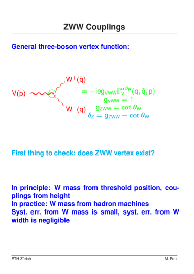
Figure 17: Three gauge boson vertex

The effect of anomalous trilinear gauge couplings is a modification of the WW production cross section and a distortion of the event kinematics.

In particular, the study of these couplings is performed with a combined fit to the total WW production cross section as well as the distribution of the production and decay angle of each W boson (see figure 18).

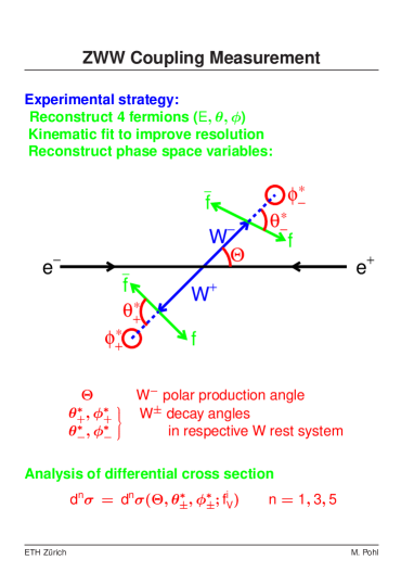
Figure 18: Production and decay angles in a WW event

If no jet charge algorithm is used, the W production angle can only be unambiguously determined in semileptonic events, where the charge of the lepton reflects the charge of the parent W. In the fully leptonic case, all production and decay angles can be determined with a two-fold ambiguity using kinematic criteria if initial state radiation and W width are neglected ^?. In the four-jet channel the ambiguity on the angles can only be solved using the jet charge. Algorithms based on the Feynman-Fields approach ^? have correct charge identification probability around 70%.

Detector effects in angle resolution and charge confusion are accounted for using reweighting algorithms similar to those used for the measurement of the W mass. An alternative approach is that based on Optimal Observables ^?. Instead of fitting the kinematic distributions, the differential cross section parametrized as a quartic function of the anomalous couplings:

$$\frac{d\sigma}{d\Omega}=c_{0}(\Omega)+c_{1}(\Omega)\Psi+c_{2}(\Omega)\Psi^{2}$$

where $\Omega$ are the phase space variables, and $\Psi$ is one of the couplings allowed to be different from the standard model, while the others are kept to zero. Assuming that all couplings are small, it is possible to neglect the term $c_{2}$, and apart from this approximation the observable

$$O_{1}=\frac{c_{1}(\Omega)}{c_{0}(\Omega)}$$

contains all the information carried by the distributions $d\sigma/d\Omega$, allowing the extraction of the couplings from a 1-dimensional fit.

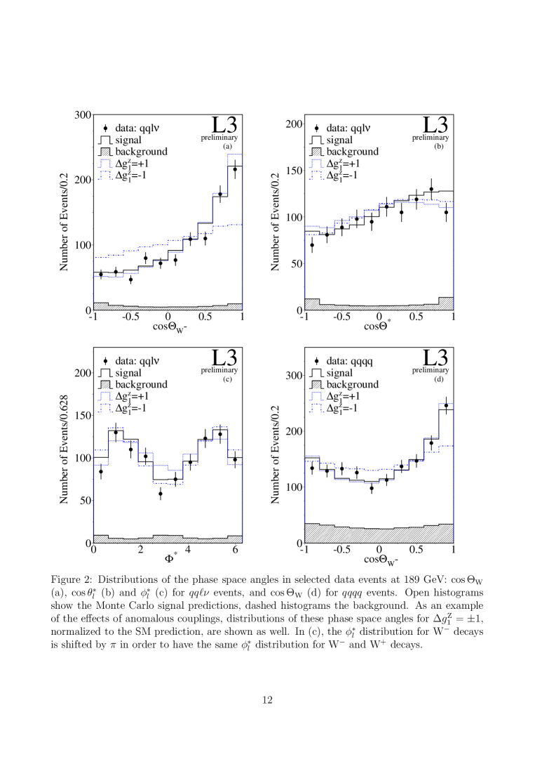
Figure 19: Distributions of production and decay angles in L3 WW events at 189 GeV

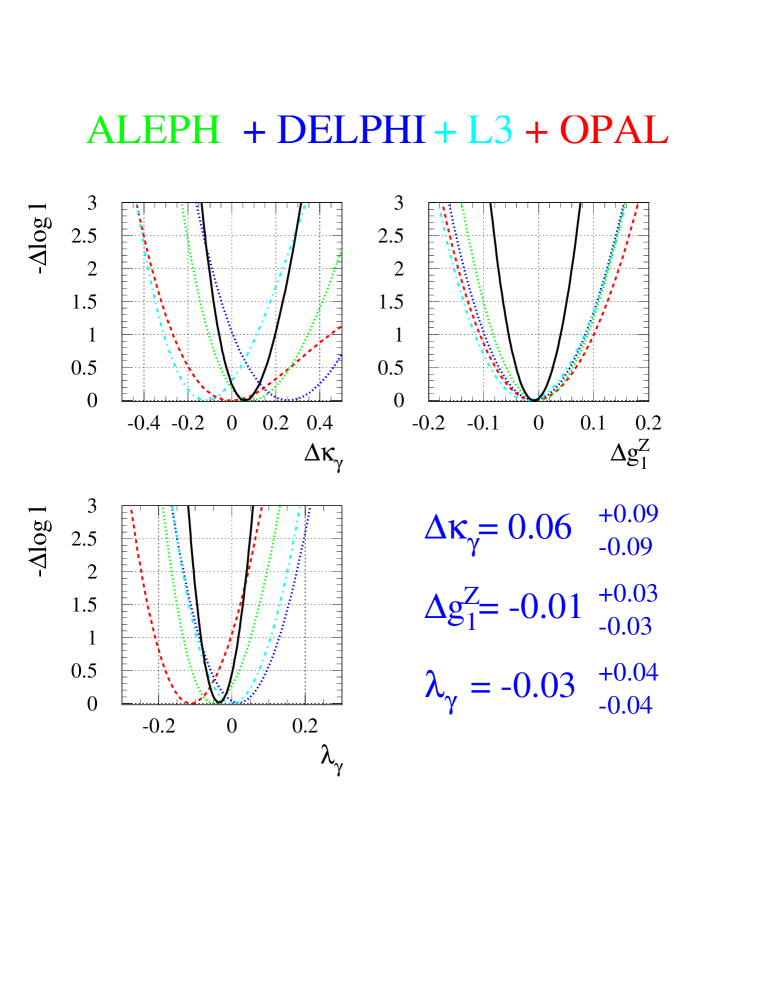
Figure 20: Values of single coupling variables obtained combining the four LEP experiments, assuming the other variables set to the standard model value. The four curves in each plot correspond to the results of the four LEP experiments.

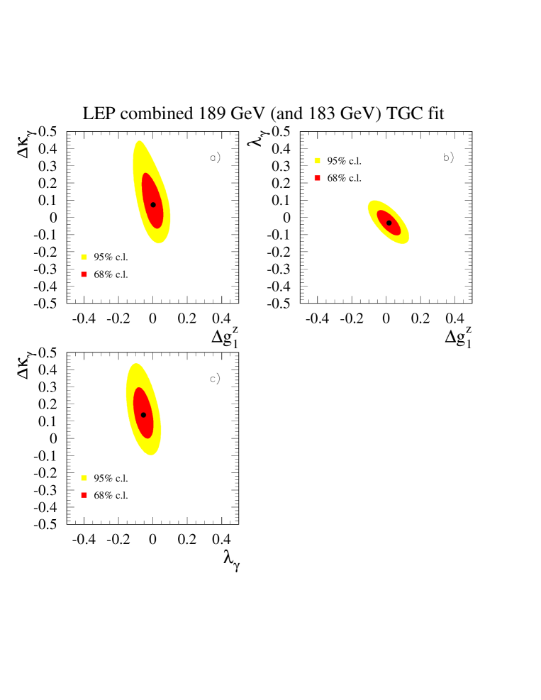
Figure 21: Combined allowed contours for TGC variables when one is set to the standard model value and the other are left as free parameters of the fit.

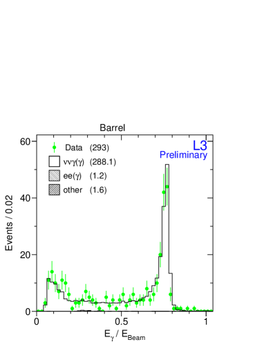
Figure 22: Energy spectrum of single photon events in L3 for 189 GeV data

Diagrams involving the interaction of three vector bosons are not only present in WW final state events, but also in other kind of processes, e.g. production of single W and single photons (figure 22. With respect to WW production, these processes are more sensitive to $\gamma WW$ couplings, $\Delta\kappa_{\gamma}$ and $\Delta\lambda_{\gamma}$.

As discussed above, all analyses performed to study trilinear gauge couplings are based on reconstructed distributions of W decay products (or photon). The final sensitivity of the result strongly depends on the reconstruction performances for these quantities, therefore also in this case kinematic fits are widely used. The main sources of systematics are coming from the accuracy of the MonteCarlo modeling of detector effects, as well as the effects in fragmentation as well as final-state hadronic interactions, as already discussed for the case of the W mass measurement.

Final results for the couplings can be expressed in terms of one variable constraining the others to the standard model values, or fitting two variables at the same time. The LEP combined results following these two approaches are shown in figures 20 and 21. Results from the single experiments can be found in the references ^?.

11 QCD effects

Hadronic interactions occur between W decay products, and can lead to modification of the observed final states. In particular the understanding of these effects is very important for the W mass measurement, since they can lead to biases in the 4-jet channel far larger than the target accuracy for this measurement. In particular, Bose-Einstein and color reconnection effects will be discussed.

11.1 Bose-Einstein effects

Bose-Einstein correlations enhance the production of identical bosons close in direction and momentum. These effects have already been observed in nucleus-nucleus and hadron-hadron interactions^?, as well as in hadronic Z decays at LEP1 ^?.

In WW events, Bose-Einstein correlations can occur:

• between bosons within same jet

• between bosons from same W

• between bosons from different Ws

Only the last case is important for W mass studies, since it generates distortions in the reconstructed invariant mass spectrum.

Figure 23: R(Q) distribution from DELPHI data at 183 and 189 GeV. (a): in semileptonic events. (b) in fully hadronic events, compared to a model with full BEC. (c) same data as in (b), compared to a model with BEC only inside the same jet. Data seem favoring models with full BEC.

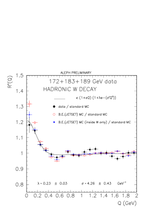
Figure 24: Data/MC ratio of R(Q) distributions in ALEPH. Data (full dots) are in better agreement with MonteCarlo where BEC occur only inside the same W (stars) than in models where they occur between different Ws (open dots)

To model this effect, the correlation function between two equal bosons is assumed to be Gaussian:

$$R(Q)=(1+\lambda e^{-Q^{2}R^{2}})$$

where $\lambda$ and R are the amplitude and the radius of the effect, and Q is the four-momentum difference between the two identical bosons $Q^{2}=(p_{1}-p_{2})^{2}$.

From the experimental point of view, most of the effect shows up between pions of the same charge inside hadronic jets, while pions of different charge are not affected. Bose-Einstein correlations produces an enhancement in the ratio of the Q distribution between same-sign ($\rho^{\pm\pm}$) and opposite-sign ($\rho{\pm\mp}$) pions:

$$R(Q)=\frac{\rho^{\pm\pm}(Q)}{\rho^{\pm\mp}(Q)}$$

The effect can either be seen from the R(Q) distribution itself (OPAL), in the double ratio $R(Q)_{DATA}/R(Q)_{MC}$ (ALEPH, L3), or defining

$$R(Q)=\frac{\rho^{\pm\pm}(Q)}{\rho^{\pm\pm}_{MC}(Q)}$$

where the Monte Carlo sample has no Bose-Einstein correlations (DELPHI).

Delphi results are slightly in favor of the presence of Bose-Einstein Correlations between particles from different Ws (figure 24), while the results from ALEPH seem disfavoring (by 2.7 $\sigma$) such correlations (figure 24).

The preliminary values for the amplitude of the effect between pions coming from different W $\lambda^{diffW}$ are listed in table 4 ^?. To be noticed that ALEPH and L3 results are preliminary, and the data sample used are widely different. With the present available information the presence of Bose-Einstein correlations between different Ws is still unclear.

Experiment	$\lambda^{diffW}$
ALEPH	$0.15\pm 0.18$
DELPHI	$-0.20\pm 0.22$
L3	$0.75\pm 1.80$
OPAL	$0.22\pm 0.53$

Table 4: Fitted values for $\lambda$

11.2 Colour reconnection

String effects between jets coming from different Ws (but from partons with opposite colour) are another source of distortion of the mass distribution. They can occur since the distance in space between the two W decay vertices is of the order of 0.1 fm, while the hadronic scale is of the order of 1 fm.

Perturbative contributions are expected to be small,^? but the non perturbative part can lead to mass shifts of the order of some hundreds MeV, depending on the model. The experimental study of these effects exploits the fact that in addition to W mass shifts, colour reconnections produce modifications in the topology of the events. The most important observable used to discriminate among the different models is the charged multiplicity in four-jet events (often expressed as difference or ratio between charged particle production in $qqqq$ and $2\times qql\nu$ events, which are not affected by CR)^?. Typically, models predicting shifts in the W mass of the order of several hundred MeV also predict a difference in the number of charged particles between semileptonic and hadronic events of about 10%, while for models leading to smaller mass shifts this difference is few per cent. As shown if figure 25, it is very difficult with present data to discriminate among the models implemented in the event generators ^?, since the predicted shift is similar and quite small.

Figure 25: Number of charged particles in 4-jet hadronic events compared to different color reconnection models. Apart from the VNI model, that fails to reproduce the thrust distribution (plot c), the other models predict very small shifts in the charged multiplicity, and the present data are not able to discriminate among them.

Table 5 shows the difference (the ratio for DELPHI) between then charged multiplicity of 4-jet events and twice the one of semileptonic events ^?. Present errors on this quantity are still too large to be compared to the existing models.

Experiment	$\Delta<n_{ch}>$
ALEPH	$0.47\pm 0.44\pm 0.26$
L3	$-.0\pm 0.8\pm 0.5$
OPAL	$0.7\pm 0.8\pm 0.6$
	$<N_{ch}^{qqqq}>/2<N_{ch}^{qq}>$
DELPHI	$0.977\pm 0.017\pm 0.027$

Table 5: Difference (ratio for DELPHI) in charged multiplicity between four-jet and two-jet events. Results from L3 and OPAL do not include 189 GeV data. Only OPAL results are final.

Other observables for studying color reconnection studies are:

• charged multiplicity in the low momentum region

• track characteristic distributions (momentum, rapidity, $p_{t}$,…)

• event shape (thrust,…)

• heavy hadron multiplicity (K,p with $0.2GeV<p<1.4$ GeV)

Also for these observables no clear indications for color reconnection can be derived.

12 Charm production in W decays

For real W bosons the production of b quarks is either forbidden by energy conservation (as in the case $W\to tb$) or strongly Cabibbo-suppressed (as in the case of the decay $W\to cb$). For this reason, charm is the heaviest quark largely produced in W decays. Using its heavy-quark characteristics in an almost b-free environment, it is possible to measure the charm production branching ratio in W decays. In the standard model this value is precisely determined by the unitarity of the CKM matrix:

$$\frac{|V_{cd}|^{2}+|V_{cs}|^{2}+|V_{cb}|^{2}}{|V_{cd}|^{2}+|V_{cs}|^{2}+|V_{cb}|^{2}+|V_{ud}|^{2}+|V_{us}|^{2}+|V_{ub}|^{2}}$$

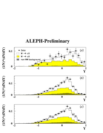
Figure 26: Distribution of the Fisher Discriminant for (a) semileptonic events (b) fully-hadronic events (c) the sum of the two classes

For this reason, a measurement of the charm fraction in W decays is a direct test of the unitarity of the CKM matrix. Furthermore, using the precise determinations of the other elements, it is possible to convert this measurement into a determination of $|V_{cs}|$.

This approach to the determination of this matrix element is less precise than the derivation from the hadronic branching ratio, but more direct. For charm tagging, the three experiments performing this measurement use different experimental techniques:

• ALEPH (172+183 GeV data) use a neural network with 12 input variables or a Fisher discriminator (see figure 26). Variables used come from b-tagging, event shapes, exclusive decays etc. A combination of the two methods is used for the final result.

• L3 (183 GeV data) splits jets into four categories, depending whether an inclusive lepton ( $e,\mu$ ), a $D^{*}\to D^{0}\pi^{\pm}$ or none of the above is found. Each category is then analyzed by a separate neural network.

• DELPHI (172 GeV data) exploits its RICH detector for kaon identification, thus directly measuring $V_{cs}$ through an s-tag in addition to a charm tag performed in a similar way as the other experiments.

The results obtained are summarized in table 6^?.

	$|V_{cs}|$
$D\to Kl\nu$(PDG)	$1.04\pm 0.16$
ALEPH	$1.00\pm 0.10\pm 0.06$
L3	$0.98\pm 0.22\pm 0.08$
DELPHI	$0.91\pm 0.14\pm 0.05$
LEP direct	$0.96\pm 0.09$
LEP BR(W$\to$qq)	$1.03\pm 0.04$
CKM unitarity	$0.9745\pm 0.0005$

Table 6: Determinations of $|V_{cs}|$

13 Conclusions

After three years of data taking above the WW threshold, W physics at LEP has reached the realm of precision measurements. Data have been collected at 161, 172, 183 and 189 GeV of center of mass, with increasing integrated luminosity. The selection of WW events provides measurements of the WW total cross section and of the branching ratios of all decay channels. All these measurement are in agreement with the predictions from the standard electroweak theory. A sector where deviation from the standard theory could be expected is the study of the trilinear gauge coupling. Fits to the cross section and to the kinematics of the events so far are in agreement with the expectations, so limits on the presence of anomalous couplings are established. Charm production in W decays provides a direct determination of $|V_{cs}|$, while an indirect measurement can be derived from the hadronic branching fraction. The most important measurement in W physics at LEP is the W mass. After a derivation from the threshold cross section in the first run, the mass is now measured using the direct reconstruction of the invariant mass of the W decay products. The present combined result $M_{W}=80.368\pm 0.065$ is as precise as the one obtained from hadronic machines, and its accuracy will further improve in the next years. The question is still open on whether the accuracy on the W mass will be finally dominated by systematic uncertainties. Some systematic errors are likely to considerably improve with more study, but the large uncertainties associated with QCD interactions in the four jet channel may be not so easy to reduce, and limit the final accuracy of the result.

LEP2 will run for two more years, aiming to reach the design integrated luminosity of 500 $pb^{-1}$ and trying to reach the centre-of-mass energy of 200 GeV. W physics will fully profit from more data and from more energy points, and the results from the four LEP experiments will increase their sensitivity both in the measurement of the parameters of the standard theory and in the search for new phenomena.

14 Acknowledgements

I would like to thank M. Pohl for having introduced me to the field of W physics. Many thanks also to M.Grunewald, L.Malgeri and A.Tonazzo and for careful reading of the manuscript and A.Rubbia for the encouragement.

References

References

-
[1]
S.L. Glashow, Nucl. Phys. 22 (1961) 579;
S. Weinberg, Phys. Rev. Lett. 19 (1967) 1264
A. Salam, in Elementary Particle Theory, ed. N.Svartholm (Stockholm, 1968) p.367
for reviews, see G.Barbiellini, C.Santoni, Riv. Nuovo Cimento, 9(2), 1 (1986)
-
[2]
UA1 proposal, CERN/SPSC 78-06 (1978)
M.Barranco Loque at al., NIM 176 175 (1980)
M.Calvetti et al., NIM 176 255 (1980)
K.Eggert et al. NIM 176 217-233 (1980)
A.Astbury, Phys. Scr. 23 397 (1981) - [3] M.Banner ıet al. UA2 collab. Proc. Int. Conf. on Instrumentation for colliding beam physics, SLAC-250 (1982)
-
[4]
G.Arnison et al (UA1 coll.), Phys. Lett. B 122 103
(1983)
M.Banner et al. (UA2 coll.), Phys. Lett. B 122 476 (1983)
G.Arnison et al. (UA1 coll.), Phys. Lett. B 126 398 (1983) -
[5]
F.Abe et al CDF coll., Phys. Rev. Lett. 75 11 (1995)
D0 coll. preliminary results presented by C.K.Jung at 27th ICHEP, Glasgow 1994 - [6] G. Altarelli et al. Physics at LEP2 CERN report 96-01 (1996 )
-
[7]
P.W. Higgs, Phys. Lett. 12, 132 (1964), Phys. Rev.
Lett. 13, 508 (1964), Phys. Rev. 145, 1156 (1966)
F.Englert and R.Brout, Phys. Rev. Lett. 13, 321 (1964)
G.S. Guralnik, C.R. Hagen, T.W.B. Kibble, Phys. Rev. Lett. 13, 585 (1964) E.D. Commins and P.H. Bucksbaum, Weak interactions of leptons and quarks (Cambridge University Press, Cambr., 1983) - [8] G.Burgers, F.Jegerlehner, in “Z physics at LEP1”, CERN, 89-08 (1989) p. 55
-
[9]
LEPEWWG plots for winter conferences. See for instance
http://www.cern.ch/LEPEWWG/plots/winter99/ - [10] G.Gounaris ıet al., in “Physics at LEP2”, CERN, 96-01 (1996) p. 525
- [11] The LEP working group on Four Jets, “Report of the LEP Working Group on four-jet production in collisions at centre-of-mass energies of 130-172 GeV”, Internal Note, ALEPH 97-056, DELPHI 97-57, L3 2090, OPAL TN 486 (June 1997) and references therein.
- [12] “Calibration of centre-of-mass energies at LEP1 for precise measurements of Z properties”, LEP Energy Working Group, Eur. Phys. J. C6 (1000) 2, 187-223.
-
[13]
ALEPH 99-020 CONF 99-015
DELPHI 99-39 CONF 238
L3 Note 2376
OPAL PN 378 - [14] The 1998 Review of Particle Physics: C. Caso et al, The European Physical Journal C3 (1998) 1
-
[15]
ALEPH 99/017 CONF 99/012
L3 Note 2377
OPAL CERN-EP/98-197 and D.Glenzinski (LEPC 24/03/99)
DELPHI 99-41 CONF 240 and N.J.Kjaer (LEPC 24/03/99)
-
[16]
ALEPH CONF 99/014
L3 note 2049 - [17] R.D.Field, R.P.Feynman Nucl. Phys. B 136 1 (1978)
-
[18]
Phys. Lett. B 305 (1993) 219;
Z. Phys. C 52 (1994) 397 -
[19]
ALEPH 99-019 CONF 99-014
ALEPH 99-021 CONF 99-016
ALEPH 99-025 CONF 99-019
DELPHI 99-36 CONF 235
L3 Note 2378
OPAL PN 375 - [20] G.Goldhaber et al., Phys. rev. 120 (1960) 300.
-
[21]
ALEPH coll. Z.Phys. C54 (1992) 75.
DELPHI coll. Phys. Lett. B286 (1992) 201.
-
[22]
ALEPH 99-027 CONF 99-021
DELPHI 99-22 CONF 221
L3 Note 2268
OPAL PR 262 OPAL coll. Z.Phys. C72 (1996) 389. - [23] T.Sjostrand and V.A. Khoze, Z.Phys. C 62 (1994); Phys. Rev. Lett. 72 (1994) 28.
- [24] G.Gustafson, U.Pettersson and P.M. Zerwas, Phys. Lett. B209 (1988) 90.
-
[25]
PHYTHIA T.Sjöstrand and V.A. Khoze, Z.Phys. C 62 (1994)
281; Phys. Rev. Lett. 72 (1994) 28.
ARIADNE L.Lönnblad Z.Phys. C70 (1996) 107.
HERWIG G.Marchesini et al. Comput. Phys. Commun. 67 (1992) 465.
J.Ellis, K.Geiger, Phys. Rev. D 54 (1996) 1967.
K.Geiger Comput. Phys. Commun. 104 (1997) 70.
-
[26]
ALEPH 99-027 CONF 99-021
DELPHI 99-22 CONF 221
L3 Note 2268
OPAL PR 262 -
[27]
ALEPH 98-011 CONG 98-001
DELPHI Phys. Lett. B 439 (1998) 209
L3 Note 2232