Mixing and -Violation Measurements of Mesons from the Tevatron Collider
Abstract
mixing measurements from the Tevatron Run I data are reported. These include time-integrated measurements of the average mixing parameter , six time-dependent oscillation measurements of , and a time-dependent limit on . Such measurements provide constraints on CKM matrix elements. A sample of decays is used to directly measure the -violation parameter . This value agrees well with indirect constraints on the CKM matrix.
FERMILAB-CONF-99/042-E
1 -Physics and the CKM Matrix
A major objective in the study of bottom hadrons is determining the elements of the Cabbibo-Kobayashi-Maskawa (CKM) matrix [1], and to stringently test its adequacy. This matrix transforms the flavor eigenstates of quarks into their mass eigenstates, which are not the same in the Standard Model (SM). A convenient parameterization in powers of the Cabibbo angle () is due to Wolfenstein [2]:
The imaginary term was conjectured by Kobayashi and Maskawa to be the source of violation, which has been an outstanding issue for the last 35 years.
Constraints on the CKM matrix from the -sector initially came from lifetime and branching ratio measurements in the early ’80’s. In 1986, a new window was opened by the observation of - mixing in an unresolved mixture of and by UA1 [3] in collisions, and subsequently for pure ’s by ARGUS [4] at the . Through mixing, one gains access to the CKM elements, an important consideration given the limitations of direct top studies.
Global fits to experimental data constrain the four parameters of the CKM [5, 6], with and already known quite well. Constraining and has been the recent focus of -physics. One of the unitarity constraints (), is graphically represented in Fig. 1 as a triangle in the complex - plane, with the apex at (,). Its base is of unit length, leaving three angles and two sides that may be measured. - mixing constrains the right leg (), and violation in decays determines the angle .
Mixing studies of mesons have greatly advanced in the ’90’s, and we are entering a new stage at the close of the millennium with the advent of -violation measurements in mesons. The contributions from the Fermilab Tevatron Collider program to these efforts from Run I (1992-6) data are discussed. The two collider experiments, CDF [7] and DØ [8], are well known, and their descriptions are not repeated here.
2 - Mixing Measurements
2.1 Mixing and Flavor Tagging
Like the - system, 2nd order weak “box” diagrams result in oscillations between and mesons. The frequency is the mass difference () between the heavy/light mass eigenstates and . The dominant effect arises from diagrams with virtual top quarks, with for mesons. Thus, constrains the CKM element relating transitions between top and the light quark composing the , and relates to the right leg of the unitarity triangle (Fig. 1). The probability that an initially pure state decays as a (and vice versa) at proper time is . The asymmetry between the mixed () and unmixed () states is therefore
| (1) |
Observing mixing is predicated upon determining the “flavor”—whether the is composed of a or a quark—at the times of production and decay. The decay flavor is usually known from the reconstruction. More problematic is tagging the initial flavor. If this is correct with probability , then the observed asymmetry is attenuated by the “dilution” , i.e. . A tagger with efficiency yields an error on the asymmetry which scales as for background-free mesons, and thus measures the tagger’s effective power.
2.2 Time-Integrated Mixing Measurements
It is not necessary to measure the proper decay time to observe mixing, since
| (2) |
is nonzero. At the Tevatron both and are produced, and unless one explicitly identifies the -species one measures an average , for fractions and of the and contributions.
CDF and DØ have measured using dileptons, where the leptons identify both the and tag its flavor. Like-sign pairs indicate that one -hadron has mixed. In pb-1 of dimuon triggers ( GeV/) DØ found 59 like-sign (LS) and 113 unlike (US) pairs. The ratio is used in conjunction with models of other processes ( sequential decays, , fake leptons,…etc.) to extract [9]. Similarly, CDF has used pb-1 of dimuons to obtain [10]; and in - events [11]. All agree with from the PDG [12].
2.3 Time-Dependent -Mixing Measurements
With the advent of precision vertex detectors direct observation of the oscillation has overshadowed the analyses. The DØ detector will have such tracking capability starting in Run II [13], and such studies have been restricted to CDF in Run I. Six analyses have been reported ( pb-1), and are summarized in Fig. 2.
Two analyses are extensions of the time-integrated measurements described above: dilepton samples (, ) are used where the leptons define both the signal and its flavor. In this case a secondary vertex associated to a lepton is sought to establish the -decay vertex. Average corrections transform the observed momentum and decay length into the proper decay time. The inclusive nature of the selection allows other processes to contribute (, fakes, etc.…). Their contributions to the sample are constrained by kinematic variables, such as the relative of the lepton to other parts of the decaying . The samples are more than 80% pure . The oscillation is revealed in the time variation of the like-sign dilepton fraction, and fits extract (see “” [14] and “” in Fig. 2).
In another dilepton analysis [15] the is more cleanly identified by reconstructing a near a lepton. From the lepton on the other side one infers the initial flavor of the meson. The oscillation from a signal of events is shown in Fig. 2 under “lep/lep,” along with its . The cleanliness of the sample results in a small systematic error (), but at the price of worse statistical precision.
Inclusive lepton triggers ( and , GeV/) are used to obtain a tagged sample, where the flavor on the opposite side is identified by reconstructing a . The resulting oscillation for events is labeled as “/lep” in Fig. 2 [16].
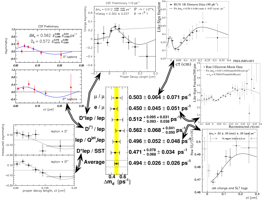
We next consider the “lep/lep” analysis [17], which again uses a lepton+vertex to identify a -hadron and a second lepton as a tag. It also uses the subtle technique of “jet-charge” tagging. The sample arises from inclusive lepton triggers, where we search for another lepton as a tag similar to the earlier analyses. We do not dwell on this aspect. More interesting is the use of “jet-charge” tagging, where an average charge of a jet opposite the +vertex is used to infer the initial flavor of the -hadron producing the trigger lepton. The charge of the away-side jet is defined as
| (3) |
where and are the charge and momentum of the -th track in the jet, and is the unit vector pointing along the jet axis. A negative (positive) implies the jet contained a (). One finds that the tag purity is higher for larger . The sample composition is again determined via kinematic variables like the of the trigger lepton and the invariant mass of the secondary vertex. The fit results of the tagging asymmetry for million events are given in Fig. 2 as “lep/lep.”
The sixth analysis uses “Same-Side Tagging” (SST), where a track near the reconstructed tags its flavor [18], rather than using the other -hadron. The idea is simple. A quark hadronizing into a picks up a in the fragmentation, leaving a . To make a charged pion, the picks up a making a . Conversely, a will be associated with a . Correlated pions also arise from decays. Both sources have the same correlation, and are not distinguished here.111 A recent CDF analysis of a sample found the fraction of mesons arising from states to be [19]. mesons are indeed a significant source of correlated pions.
CDF adopted a “” algorithm, where the tag is the candidate track with the smallest momentum component transverse to the +Track momentum. A charged particle is a valid SST candidate if it is reconstructed in the Si-vertex detector (SVX), has MeV/, is within of the , and its impact parameter is within of the primary vertex.
SST is applied to almost 10,000 events reconstructed via four decay signatures and one for [20, 21]. The sample composition is unraveled in the fit (including cross-talk). The fit results are shown in Fig. 2 as “lep/SST,” with the upper plot showing the reconstruction and the lower one is for . Along with , one also obtains the dilution, , of this SST method. This analysis provides the dilution calibration for the SST analyses of Sec. 3.
The six results are combined, accounting for correlations, into a CDF average of ps-1. This is comparable to other experiments, and is in good agreement with the PDG value of ps-1 [12].
2.4 Time-Dependent -Mixing Measurements
mixing follows the same formalism as for ’s, except the relevant CKM element is rather than . Measurements of (Sec 2.2), along with measured at the and estimates for the species fractions and , provided the original direct indication that is close to its asymptotic limit () and thereby insensitive to . Further progress on mixing necessitates time-dependent methods.
CDF has searched for oscillations [22] using dileptons (110 pb-1 of or ) for , where is a charged track associated to a decay vertex. This signature selects , ; exclusive reconstruction is not required to increase statistics. The resulting mass distribution is shown in Fig. 3. The decay point is obtained by projecting the decay back to the . Monte Carlo corrections are applied to the factor for the proper time estimation. A sample of candidates (purity of %) is obtained.
The flavor is inferred from the other trigger lepton, similar to the analyses. Events are again classified as “unmixed” () or “mixed” (). Limits will be set rather than an observation of the oscillation, so one must know a priori the mistag rate . This was found to be from a likelihood fit of the mixed/unmixed fractions in the data. The oscillation is too rapid to influence the determination of ; rather it is governed by the sample contributions of , , , sequential decays and fake background.
The data are fit with an unbinned likelihood to describe the mixed versus unmixed components. The fit includes the various sources of events (, , ,…) and is a free parameter. No oscillation is observed, and limits are set. The amplitude method [23] is adopted, whereby the functional form of is replaced by , i.e. the amplitude is a free -dependent parameter. For the true value , , and otherwise . The result of the scan of from the likelihood is shown in Fig. 3. The data fluctuate about zero, with no evidence for an oscillation. Values of are excluded at the 95% CL if , and thus ps-1 at 95% CL accounting for both statistical and systematic errors (Fig. 3, solid line).
This result is competitive with other single tagging measurements. However, the world limit, ps-1 (95% CL), is dominated by the multi-tag results from ALEPH and DELPHI [24].
It is conceivable that oscillations are too rapid to be directly observed. If so, the width difference between the mass eigenstates is expected to be large. CDF has searched for two lifetime components in a sample, and finds at 95% CL [25]. Given and the mean lifetime , this can be expressed as the upper bound at 95% CL., with a recent estimate [26]. The limit is weak, but with the increased statistics of Run II either or should be directly determined.
3 Violation in
The origin of violation has been an outstanding question since its unexpected discovery in 35 years ago [27]. In 1972, before the discovery of charm, Kobayashi and Maskawa [1] proposed that this was the result of quark mixing with 3 (or more) generations. Unfortunately the has been the only place violation has been observed. Despite precision -studies, a complete picture of violation is still lacking; and it is often argued that the CKM model can not be the full story [28].
-violation searches have encompassed mesons, but the effects in inclusive studies [10, 29] are too small () to as yet detect. In the early ’80’s it was realized [30] that the mixing interference of decays into the same state could manifest large violations. Unfortunately these decays were, until recently, too rare to study.
The “golden” mode for observing large violation in ’s is ,222 Another mode of possible interest is . While this is not a eigenstate, it can be decomposed into even and odd eigenstates by an angular analysis. This has been done by CDF for (and ) to extract the decay matrix elements [31], but the Run I statistics are insufficient to be of interest for measuring -violation parameters. and, critically, it is related to the CKM matrix with little theoretical uncertainty. A may decay directly to , or the may oscillate into and then decay to . These two paths have a phase difference, quantified by the angle of the unitarity triangle (Fig. 1). This gives rise to a decay asymmetry
| (4) |
where [] is the number of decays to at proper time given that the meson was a [] at . OPAL investigated violation with 24 candidates (60% purity), and obtained [32]. CDF has taken advantage of the large cross section at the Tevatron and obtained a sample of several hundred decays to to measure [33].
3.1 Same Side Tagging Analysis of
candidates are selected from the sample (110 pb-1). A time-dependent analysis demands that both muons are in the Si-vertex detector (SVX), cutting away half of the ’s. The reconstruction tries all tracks, assumed to be pions. The must be above 0.7 GeV/, its decay vertex displaced from the ’s by more than , and GeV/. We construct , where is the fitted mass, its error (), and is the central mass. The distribution for candidates with is shown in Fig. 4a. A likelihood fit yields (for all ) ’s.
The initial flavor is tagged by the identical SST of the measurement of Sec. 2.3. SST is independent of the decay mode, and therefore the dilution measurement can be transferred from one mode to another. However a small kinematic correction, determined from Monte Carlo, is made to translate the dilution to the sample due to the different ranges [21]. The appropriate is [33], where the first error is due to the dilution measurements, and the second is due to the translation to the sample.
The SST method is applied to the sample, with a resultant tagging efficiency of . Analogous to Eq. (4), we compute the asymmetry
| (5) |
where are the numbers of positive and negative tags (implying and respectively) in a given -bin. Signal and sideband regions are defined as and , and the sideband-subtracted asymmetry of Eq. (5) is plotted in Fig. 4c. The dashed curve is a fit of ) to the data, with fixed to [34]. The amplitude, , measures attenuated by the dilution . Due to the shape the fit amplitude is driven by the asymmetries at larger ’s, where backgrounds are small (see Fig. 4b).
The fit is refined using an unbinned likelihood fit. This makes optimal use of the low statistics by fitting the data in and , including sideband and events which help constrain the background. The fit also incorporates resolutions and corrections for (small) systematic detector biases. The solid curves in Fig. 4a,c are the result of the likelihood fit, which gives . As expected, both fits give similar values since the result is dominated by the sample size. The systematic uncertainty on is 0.03, dominated by the uncertainty on ( ps-1), but includes the effects from detector biases and the lifetime.
To extract from the measured asymmetry the dilution must be divided out. However, as long as , the exclusion of is independent of further knowledge of . Given , the unified frequentist approach of Feldman and Cousins [35] yields a dilution-independent exclusion of at 90% CL.
From above, , which results in . The central value is unphysical since the amplitude of the raw asymmetry is larger than . This result corresponds to excluding at a 95% CL.
3.2 Multi-Tagging Analysis of
Shortly after this conference CDF released an expanded analysis using three taggers, as well as non-SVX data. These preliminary results are briefly summarized.
The above SST result is statistically very limited. It can be improved by increasing the effective statistics by using lepton and jet-charge tagging to increase the total . The raw statistics can also be increased by utilizing the candidates not reconstructed in the SVX. Precision lifetime information is lost, reducing the power of these events, but significant information remains. The selection is otherwise similar to the SST-only analysis, and results in a total of candidates ( in the SVX, are non-SVX).
SST, lepton, and jet-charge tagging are applied to this sample. Lepton tagging follows the analyses. The jet-charge algorithm is similar to the analysis but uses a “mass” jet algorithm rather than a “cone” based one. This improves the efficiency for identifying low- “jets” for the tag. A lepton tends to dominate the jet charge if a lepton tag is in the jet. Since lepton tagging has low efficiency but high dilution, the correlation between lepton and jet-charge tags is avoided by dropping the jet-charge tag if there is a lepton tag. The dilutions of these two methods are measured in decays (Table 1), and are directly applicable to the sample. The precision is not high, but this obviates the complex problem of translating dilutions from kinematically different samples.
The tagged events are fit in an unbinned likelihood fit ( constrained to ps-1 [12]). The results for the individually tagged subsamples are listed in Table 1,
| Tagger | Eff. (%) | Dil. (%) | |
|---|---|---|---|
| SST | |||
| SST | |||
| Lepton | |||
| Jet- | |||
| Global | |||
including systematic errors due to the dilutions, , , and . The SST result is slightly larger than before with the inclusion of the non-SVX events, and the error has decreased by %. The other two taggers fall in the physical range, one positive and the other negative.
Rather than average these three results, the likelihood fitter is generalized to fit all three simultaneously while accounting for tag correlations. The global multi-tag result is (Fig. 5), including the systematic uncertainties. This result corresponds to a unified frequentist confidence interval of at 93% CL. Although the exclusion of zero has only slightly increased from 90% for the (SVX) SST-only analysis, the uncertainty on is cut in half.
4 Summary and Prospects
Measurements of and provide important constraints on the CKM matrix. World averages constrain the triangle of Fig. 1 quite well, as shown in Fig. 6. An indirect determination of was reported at this conference [6]. This is much more precise than the direct CDF measurement; nevertheless, the agreement is an auspicious omen for the CKM model’s account of violation.
Additional sources of violation are, however, thought necessary to account for the baryon asymmetry in the universe [28]. Searching for physics beyond the CKM model demands stringent tests, and is the focus of dedicated factories. Both CDF and DØ will also be fully engaged in this effort by exploiting the rich harvest from Run II. Commencing in 2000, a two-year run will deliver the luminosity ( fb-1), to be exploited by greatly enhanced detectors. With the “baseline” detector and trigger upgrades [13, 36] CDF projects 10,000 dimuon triggers for a error of about ; and DØ, with a new precision tracking system, expects an error of 0.12-0.15 (Fig. 6). Dielectron triggers may further increase the samples by %. These errors are in the range projected for factories. The Run II Tevatron will be competitive in many other areas of physics as well.
oscillations have, so far, eluded all comers. The Tevatron should have a virtual monopoly on the after the closure of the machines and before the start of the LHC. Run II baseline expectations are for CDF to reach ’s up to 30-40, and DØ up to 20-25. Although DØ’s reach is less, it is sufficient that failure to observe oscillations should critically challenge the CKM model.
In addition to the baseline upgrades, both experiments are aggressively pursuing further improvements. For example, CDF is working towards an additional Si-layer to improve vertex resolution and a Time-of-Flight system, which may push out to ; and DØ is looking at a displaced-track trigger to greatly enhance triggering.
We close with the CKM model unscathed, but look forward to an exciting future where, perhaps, some of the mystery surrounding violation may be unveiled.
Acknowledgments
I would like to thank my fellow collaborators, and colleagues across the ring, for the pleasure of representing them and their work. Assistance with this presentation from T. Miao, M. Paulini, C. Paus, F. Stichelbaut, and J. Tseng is appreciated.
References
- [1] N. Cabibbo, Phys. Rev. Lett. 10, 531 (1963); M. Kobayashi and K. Maskawa, Prog. Theor. Phys. 49, 652 (1973).
- [2] L. Wolfenstein, Phys. Rev. Lett. 51, 1945 (1983).
- [3] UA1 Collaboration, C. Albajar et al., Phys. Lett. B 186, 247 (1987).
- [4] ARGUS Collaboration, H. Albrecht et al., Phys. Lett. B 192, 245 (1987).
- [5] S. Mele, CERN-EP/98-133, hep-ph/9810333.
- [6] A. Ali, Proc. of the 13th Topical Conference on Hadron Collider Physics, January 1999, Mumbai, India.
- [7] CDF Collaboration, F. Abe et al, Nucl. Instrum. Methods A 271, 387 (1988); P. Azzi et al, Nucl. Instrum. Methods A 360, 137 (1995).
- [8] DØ Collaboration, S. Abachi et al, Nucl. Instrum. Methods A 338, 185 (1994).
- [9] S. Feher (DØ Collaboration), Proc. of the 10th Topical Workshop on Proton-Antiproton Collider Physics, Batavia, 1995, AIP Conf. Proc. Vol. 357, 1996.
- [10] CDF Collaboration, F. Abe et al, Phys. Rev. D 55, 2546 (1997).
- [11] F. Bedeschi, (CDF Collaboration), Proc. of the 10th Topical Workshop on Proton-Antiproton Collider Physics, Batavia, 1995, AIP Conf. Proc. Vol. 357, 1996.
- [12] Particle Data Group, C. Caso et al, Eur. Phys. J. C 3, 1 (1998).
- [13] DØ Collaboration, FERMILAB-Pub-96/357-E, 1996.
- [14] CDF Collaboration, F. Abe et al, FERMILAB-PUB-99/030-E.
- [15] T. Kuwabara, Ph.D. dissertation, University of Tsukuba, 1997.
- [16] S. C. Van Den Brink, Ph.D. dissertation, University of Pittsburgh, 1998.
- [17] CDF Collaboration, F. Abe et al, FERMILAB-PUB-99/019-E.
- [18] M. Gronau, A. Nippe, and J. Rosner, Phys. Rev. D 47, 1988 (1993); M. Gronau and J. Rosner, ibid. 49, 254 (1994).
- [19] D. Vucinic, Ph.D. dissertation, Massachusetts Institute of Technology, 1999.
- [20] CDF Collaboration, F. Abe et al, Phys. Rev. Lett. 80, 2057 (1998).
- [21] CDF Collaboration, F. Abe et al, Phys. Rev. D 59, 032001 (1999).
- [22] CDF Collaboration, F. Abe et al, FERMILAB-PUB-98/401-E.
- [23] H.-G. Moser and A. Roussarie, Nucl. Instrum. Methods A 384, 491 (1997).
- [24] F. Parodi, Proc. of XXIX International Conf. on High Energy Physics, July 1998, Vancouver, B.C., Canada.
- [25] CDF Collaboration, F. Abe et al, Phys. Rev. D 59, 032004 (1999).
- [26] M. Beneke, G. Buchalla, and I. Dunietz, Phys. Rev. D 54, 4419 (1996).
- [27] J.H. Christenson et al, Phys. Rev. Lett. 13, 138 (1964).
- [28] A. Riotto and M. Trodden, hep-ph/9901362, to be published in Annual Review of Nuclear and Particle Science, Vol. 49, December 1999.
- [29] CLEO Collaboration, J. Bartelt et al, Phys. Rev. Lett. 71, 1680 (1993); OPAL Collaboration, K. Ackerstaff et al, Z. Phys. C 76, 401 (1997); OPAL Collaboration, G. Abbiendi et al, CERN-EP/98-195.
- [30] A.B. Carter and A.I. Sanda, Phys. Rev. Lett. 45, 952 (1980); I.I. Bigi and A.I. Sanda, Nucl. Phys. B 193, 85 (1981).
- [31] S. Pappas (CDF Collaboration), Proc. of DPF ’99, Jan 1999, Los Angles, CA.
- [32] OPAL Collaboration, K. Ackerstaff et al, Eur. Phys. J. C 5, 379 (1998).
- [33] CDF Collaboration, F. Abe et al, Phys. Rev. Lett. 81, 5513 (1998).
- [34] Particle Data Group, R.M. Barnett et al, Phys. Rev. D 54, 1 (1996).
- [35] G.J. Feldman and R.D. Cousins, Phys. Rev. D 57, 3873 (1998).
- [36] CDFII Collaboration, FERMILAB-Pub-96/390-E, 1996.