Abstract

We present three preliminary results from SLD on $B$ decays: an inclusive search for the process $b\!\rightarrow\!s\>gluon$, a measurement of the branching ratio for the process $B\!\rightarrow\!D\bar{D}X$, and measurements of the charged and neutral $B$ lifetimes. All three measurements make use of the excellent vertexing efficiency and resolution of the CCD Vertex Detector and the first two make use of the excellent particle identification capability of the Cherenkov Ring Imaging Detector. The $b\!\rightarrow\!sg$ analysis searches for an enhancement of high momentum charged kaons produced in $B$ decays. Within the context of a simple, Jetset-inspired model of $b\!\rightarrow\!sg$, a limit of ${\cal B}(b\!\rightarrow\!sg)$$<7.6$% is obtained. The ${\cal B}(B\rightarrow D\bar{D}X)$ analysis reconstructs two secondary vertices and uses identified charged kaons to determine which of these came from charm decays. The result of the analysis is ${\cal B}(B\rightarrow D\bar{D}X)$= $(16.2\pm 1.9\pm 4.2)$%. The results of the lifetime analysis are: $\tau_{B^{+}}=1.686\pm 0.025\pm 0.042\;$ ps, $\tau_{B^{0}}=1.589\pm 0.026\pm 0.055\;$ ps and $\tau_{B^{+}}/\tau_{B^{0}}=1.061\pm^{0.031}_{0.029}\pm 0.027$.

1 Introduction

Detailed studies of $B$-hadron decays can provide important tests of the Standard Model. In fact, it has been suggested that the existence of several “$B$-decay puzzles” may be pointing the way to physics beyond the Standard Model [1]. The most serious of these puzzles is the the low measured value compared to theoretical expectations of the the $B$ semi-leptonic branching ratio:[2]

$${{\cal B}_{SL}={\Gamma_{semi-leptonic}\over\Gamma_{semi-leptonic}+\Gamma_{hadronic}+\Gamma_{leptonic}}}$$ (1)

Theoretical expectations of ${\cal B}_{SL}$ typically have a lower limit of 12.5% [3]. As of Summer ’97, however, the experimental measurements were much lower: the world average of measurements done at the $\Upsilon(4S)$ was $0.1018\pm 0.0040$ and at the $Z^{0}$ was $0.1095\pm 0.0032$ [2].

Since $\Gamma_{semi-leptonic}$ is well understood theoretically and $\Gamma_{leptonic}$ is very small, efforts to explain the discrepancy have focused on $\Gamma_{hadronic}$, which can be broken into three parts (assuming that Cabibbo suppressed rates are small):

$$\Gamma_{hadronic}\approx\Gamma(b\!\rightarrow\!c\bar{u}d)+\Gamma(b\!\rightarrow\!c\bar{c}s)+\Gamma(b\!\rightarrow\!sg)$$ (2)

Reducing ${\cal B}_{SL}$ to the experimentally measured value would require enhancing one or more of these components significantly above the expected value. In this paper, we describe measurements that bear on each of these three components.

1.1 SLD Capabilities and Data Set

The SLD experiment collects $Z^{0}$ decay data from $e^{+}e^{-}$ collisions at the SLAC Linear Collider with a center of mass energy of 91.28 GeV. A full description of the SLD detector may be found in [4]. SLD is well-suited for doing precision measurements of inclusive $B$-decays due to several unique characteristics. The SLC interaction point is small and stable and its position is known with an uncertainty of 5 $\mu$m transverse to the beam direction. This precise IP is complemented by SLD’s high precision CCD vertex detector, VXD3 [5]. For high momentum tracks the impact parameter resolution is $\sigma(r\phi)=11\mu$m and $\sigma(rz)=22\mu$m. Multiple scattering adds a momentum-dependent contribution of $33\mu{\rm m}/(p\sin^{3/2}(\theta))$, where $p$ is the momentum expressed in GeV/c and $\theta$ is the track polar angle. Note that the above describes the performance of the upgraded vertex detector (VXD3) installed prior to the start of the 1996 run. For the performance of the vertex detector used before 1996 (VXD2), see Reference [4]. Another important capability of SLD is the excellent particle identification provided by the Cherenkov Ring Imaging Detector [6]. $K^{\pm}$’s in the barrel region with momentum between 1 and 20 GeV/c are identified with an efficiency of 50% and a $\pi^{\pm}$ misidentification probability of 2%. Data used in these analyses was taken between 1993 and 1998. However, not all data has yet been used in all analyses. Table 1 lists the different running periods used for each analysis.

Running Period	Number of Z’s	Vertex Detector	$b\!\rightarrow\!sg$	${\cal B}(B\rightarrow D\bar{D}X)$	$\tau_{\mbox{$B^{+}$}}$,$\tau_{\mbox{$B^{0}$}}$
1993-95	150K	VXD2	Yes	No	Yes
1996-98	250K	VXD3	Yes	Yes	Yes
Spring 98	150K	VXD3	Yes	Yes	No

Table 1: The three running periods used in the analyses are listed along with the vertex detector in use for that period and whether the period was used in each of the three analyses

1.2 Analysis Techniques

All three of the analyses described in this paper make use of an inclusive $B$ reconstruction method. This method was originally developed for the SLD $R_{b}$ measurement and is described in detail in [7]. Briefly, the procedure is as follows. Well measured tracks with vertex detector hits are selected. In each hemisphere, secondary vertices are formed from these “quality” tracks using a topological vertexing technique [8]. The most significant of these vertices that is significantly displaced from the IP is chosen as the “seed”. The $B$ flight direction is then defined by the line joining the primary vertex and this secondary vertex. Additional tracks are attached to the vertex if they satisfy the following criteria.

• the 3D closest approach to the flight direction is $<$ 1mm

• the distance along the flight direction to this point, L, is $>$0.5 mm

• the $L/D>$ 0.25, where D is the secondary vertex decay distance.

These tracks, seed plus attached, are called “$B$-tracks” and a $b$-tag is formed by calculating their invariant mass assuming that each has $m_{\mbox{$\pi^{\pm}$}}$. A correction is applied to account for neutrals and missing tracks which is based on the total transverse momentum of the vertex tracks to the $B$ flight direction. Figure 1 shows a histogram of this “$P_{T}$ corrected mass”, $M_{P_{T}}$. Finally a cut on $M_{P_{T}}$ is applied at 2 ${\rm GeV/c^{2}}$. In Monte Carlo studies, this $b$ selection method had an efficiency of 35% and a purity of 98% in ’93-’95 and an efficiency of 50% and a purity of 98% in ’96-’98.

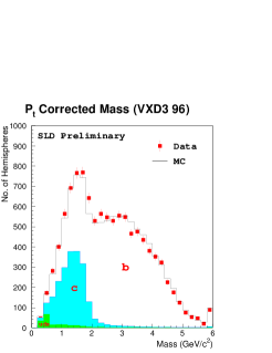
Figure 1: $P_{T}$ corrected mass for ’96 data and Monte Carlo. Cutting at $M_{P_{T}}>2{\rm GeV/c^{2}}$ gives a very pure and efficient $b$ tag.

In addition to the $M_{P_{T}}$ cut, the set of “$B$-tracks” can also be used to study the structure of the $B$ decay. This is done by fitting all $B$-tracks to a single vertex and calculating the fit probability. Due to the finite charm lifetime, $B$ decays with open charm will tend to have lower fit probability than those that are “charmless”. Decays with fit probability greater than 0.05 are called “1-Vertex” and the remaining decays are called “2-Vertex”. Table 2 shows that, indeed, decays without open charm are more likely to be in the 1-Vertex sample.

B Decay Mode	1-Vertex Fraction
Single Charm	0.33 $\pm$ 0.01
Double Charm	0.16 $\pm$ 0.02
Charmonium + X	0.76 $\pm$ 0.03
$b\!\rightarrow\!sg$ Model	0.73 $\pm$ 0.01

Table 2: Monte Carlo estimates of the fraction of $B$ decays of different types that satisfy the 1-Vertex cut.

A check is also performed on data in $B\!\rightarrow\!J/\Psi X$ data where $J/\Psi\!\rightarrow\!\mu^{+}\mu^{-}$. In these events, the 1-Vertex fraction is found to be 0.733 $\pm$ 0.094, confirming the efficiency estimated from the Monte Carlo.

2 Inclusive Search for $b\!\rightarrow\!sg$

In the Standard Model, $b\!\rightarrow\!sg$ occurs through gluonic penguins and is expected to have a total branching ratio of approximately 1% [9]. However, if the branching ratio were enhanced up to $\approx$ 10 % by some non-Standard Model mechanism, it would nicely explain the “puzzles” described in section 1 [1]. Experimentally, it has been difficult to exclude even such a large ${\cal B}(b\!\rightarrow\!sg)$ due to the lack of a clean signature for these decays.

The SLD analysis [10] searches for such a large enhancement by examining the high $p_{t}$ part of the $K^{\pm}$ spectrum, where $p_{t}$ is the momentum transverse to the $B$ flight direction. Naively, one would expect $K^{\pm}$’s produced by $b\!\rightarrow\!sg$ to have a stiffer spectrum than those produced from standard $B$ decays since they come from a direct $b\!\rightarrow\!s$ transition rather than cascade $b\!\rightarrow\!c\!\rightarrow\!s$ transitions. In a simple, jetset [11] inspired model [12] it has been verified that this is indeed the case. The model, however, is quite sensitive to the choice of tuning of jetset. Table 3 shows the number of high-$p_{t}$ $K^{\pm}$’s expected for different choices of tuning. “delphi Tuning” will be used for the rest of the analysis, but the tuning sensitivity means that limits on $b\!\rightarrow\!sg$ can be set only within the context of a particular tuning choice.

Tuning Choice	$K^{\pm}$,$p_{t}>1.8$ GeV/c per B
jetset default	$6.9\times 10^{-3}$
delphi tuning	$10.6\times 10^{-3}$
No Parton showers	$13.8\times 10^{-3}$
$b\!\rightarrow\!c$	$2.4\times 10^{-3}$

Table 3: The number of high $p_{t}$ $K^{\pm}$’s expected from $b\!\rightarrow\!sg$ for a number of different choices of jetset tunings.

In addition to the $M_{P_{T}}$ cut described above, the 1-vertex cut is also used. Since $b\!\rightarrow\!sg$ events are charmless, they are expected to be mostly one 1-vertex. Using the 1-vertex cut thus provides background rejection of standard $b\!\rightarrow\!c$ decays as well as providing a 2-vertex sample, which should not have much $b\!\rightarrow\!sg$ in it and can be used to check the background calculation. The $b\!\rightarrow\!sg$ signal should therefore show up as an enhancement in high $p_{t}$ $K^{\pm}$’s in the 1-Vertex sample. Only the high $p_{t}$ part of the spectrum is used both because it has high signal to background and also because the background in that region is well understood, leading to a small systematic error. Figure 2 shows the spectrum of $K^{\pm}$’s observed in both the 1- and 2-Vertex samples for a sample of 50623 inclusively reconstructed $B$’s. Table 4 shows the number of events expected from $b\!\rightarrow\!c$ background and the number observed in the 1-Vertex sample and for all events. The data is well described by the $b\!\rightarrow\!c$ Monte Carlo with only a small excess of high $p_{t}$ $K^{\pm}$’s observed.

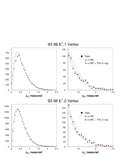
Figure 2: The $p_{t}$ spectrum of identified $K^{\pm}$’s in the 1- and 2-Vertex samples. The data is compared to $b\!\rightarrow\!c$ MC background and to $b\!\rightarrow\!c$ background plus a 10% $b\!\rightarrow\!sg$ contribution.

$K^{\pm}$,$p_{t}>1.8$ GeV/c	1 vertex		All
	Raw	Normalized	Raw	Normalized
Data	53.0	$1.46\times 10^{-3}$	150.0	$4.18\times 10^{-3}$
$b\!\rightarrow\!c$ MC	48.2	$1.29\times 10^{-3}$	132.3	$3.54\times 10^{-3}$
Difference	4.8 $\pm$ 7.3	$(1.7\pm 2.6)\times 10^{-4}$	17.7 $\pm$ 12.2	$(6.4\pm 4.4)\times 10^{-4}$
BR($b\!\rightarrow\!sg$)=10%	31.5	$1.13\times 10^{-3}$	42.2	$1.52\times 10^{-3}$

Table 4: The number $K^{\pm}$’s with $p_{t}>1.8$ GeV/c observed in data and expected from the $b\!\rightarrow\!c$ Monte Carlo with and without the 1-Vertex cut. Normalized numbers are per $B$ decay and are corrected for $K^{\pm}$ identification efficiency

The systematic error on the background rate is calculated by splitting the background high $p_{t}$ $K^{\pm}$’s into their component sources and assigning an error to each one of these sources. The largest source of background is from $K^{\pm}$’s from $D^{0}$’s that were produced in $B$-decays. This source accounts for 23.5 of the expected 48.2 background events. Fortunately, the spectrum of such $D^{0}$’s has been rather well measured [13] and the SLD $B$-decay model has been tuned to match it. This leads to a rather small systematic error of 4.3 events from this source. Other large sources of systematic error include uncertainties in the branching ratios of Cabibbo suppressed $B$ decays of the type $W\!\rightarrow\!u\!\bar{s}$ (3.6 events), $p_{t}$ smearing (4.5 events) and $K^{\pm}$ identification efficiency (3.3 events).

The preliminary result is that the excess of 1-vertex $K^{\pm}$’s with $p_{t}>1.8$ GeV/c is $4.8\pm 7.3(stat.)\pm 8.9(syst.)$ events. Within the context of the $b\!\rightarrow\!sg$ model with delphi tuning, this corresponds to ${\cal B}(\mbox{$b\!\rightarrow\!sg$})=0.015\pm 0.023\pm 0.028$. Adding the statistical and systematic errors in quadrature, this gives ${\cal B}(\mbox{$b\!\rightarrow\!sg$})<0.076$ at 90% confidence.

3 Measurement of ${\cal B}(B\rightarrow D\bar{D}X)$

Measurement of the $B$ “double-charm” branching ratio (${\cal B}(B\rightarrow D\bar{D}X)$) can help to resolve the puzzles described section 1. The SLD measurement of ${\cal B}(B\rightarrow D\bar{D}X)$ uses the same inclusive reconstruction method described above to select a set of $B$-tracks. The 2-Vertex cut is then applied - single vertex fit probability less than 0.05. The $B$-tracks in these decays are then split into two vertices using a $\chi^{2}$ minimization procedure. The upstream vertex is called the “$B$”-vertex and the downstream vertex is called the “$D$”-vertex. For single charm $B$ decays, the assignment of tracks to these vertices will tend to be correct - the $B$-vertex will contain mostly tracks coming directly from the $B$ decay and the $D$-vertex will contain mostly tracks coming from a subsequent $D$ decay. However, for double charm $B$ decays, the $B$-vertex will contain a mix of $B$ and $D$ tracks. Since $K^{\pm}$’s come primarily from $D$-decays, if a $K^{\pm}$ is found in the $B$-vertex, it is a good indication that the decay was in fact a double charm decay.

To extract ${\cal B}(B\rightarrow D\bar{D}X)$ from the data, the ratio $R_{K}$ is formed:

$${R_{K}=N_{K,B}/N_{K,D}}$$ (3)

where $N_{K,B}$ is the number of $K^{\pm}$’s observed in B-vertices and $N_{K,D}$ is number observed in D-vertices. ${\cal B}(B\rightarrow D\bar{D}X)$may then be solved for by comparing $R_{K}$ observed in data to $R_{K}$ found in Monte Carlo samples of pure double-charm and non-double-charm $B$ decays. Table 5 shows the numbers that go into this calculation.

	$N_{K^{-},B}$	$N_{K^{+},B}$	$N_{K^{-},D}$	$N_{K^{+},D}$	$N_{K,B}/N_{K,D}$
Data	1193	871	1830	1171	0.688$\pm$ 0.020
M.C. $D\bar{D}$	3068	2303	2363	1865	1.270$\pm$ 0.026
M.C. “Not-$D\bar{D}$”	5301	3903	11387	6432	0.517$\pm$ 0.007

Table 5: Number of $K^{\pm}$’s in the $B$- and $D$-vertices for data and for Monte Carlo.

Two corrections are applied to the data: background from light quark events is subtracted ($\Delta\mbox{${\cal B}(B\rightarrow D\bar{D}X)$}=$ -0.9%) and the difference in efficiency of the 2-Vertex cut between one-charm and two-charm decays is corrected for ($\Delta\mbox{${\cal B}(B\rightarrow D\bar{D}X)$}$=-5.8%).

The largest detector related systematic error comes from misassignment of tracks between $B$- and $D$-vertices. This effect is calibrated in the data using an initial state tag to identify the expected charge of leptons coming directly from the $B$ decay. “Right” sign leptons should then be found in the $B$-vertex and “wrong” sign leptons should be found in the $D$-vertex. The efficiency for correct track assignment can then be extracted from the ratio of correct to incorrect assignment. Similarly, $B\rightarrow D^{*+}X$ decays, with exclusive $D^{*+}$ decays are used to identify a set of tracks of definite origin, which are also used to measure the track misassignment efficiency. The statistical error of the track assignment efficiency is then used to calculate the systematic error due to this source, which is found to be 2.2%.

The largest physics systematics are related to $B$-decay modelling and to ${\cal B}(D\!\rightarrow\!K^{\pm}X)$. These sources lead to uncertainties of 2.1% and 1.8% respectively. The preliminary result is then ${\cal B}(B\rightarrow D\bar{D}X)$= $(16.2\pm 1.9(stat.)\pm 4.2(syst.))\%$

4 Measurement of $\tau_{B^{+}}$, $\tau_{B^{0}}$ and $\tau_{B^{+}}/\tau_{B^{0}}$

Measurement of exclusive $B$ lifetimes provides important information about $B$-hadron decay dynamics. Deviations from the naive spectator model are expected to be small and the ratio $\tau_{B^{+}}/\tau_{B^{0}}$ is expected to differ from unity by only about 10% [14]. Large deviations from unity could, for example, indicate a larger than expected value for $\Gamma(b\!\rightarrow\!c\bar{u}d)$ [15].

The SLD analysis [16] uses the same inclusive reconstruction method as described in section 1.2. In order to improve the charge purity, tracks which failed the initial quality cuts, but which still likely originated from the $B$-decay are also included. The total charge of the $B$-tracks, $Q$ is then calculated and the reconstructed $B$’s are split into a neutral sample ($Q=0$) and a charged sample (Q=$\pm$1,2,3). Figure 3 shows the distribution of $Q$ for data and Monte Carlo. Monte Carlo studies show that the ratio between $B^{+}$ and $B^{0}_{d}$ decays in the charged sample is 1.55 (1.72) for VXD2 (VXD3). Similarly, the ratio between $B^{0}_{d}$ and $B^{+}$ in the neutral sample is 1.96 (2.24) for VXD2 (VXD3).

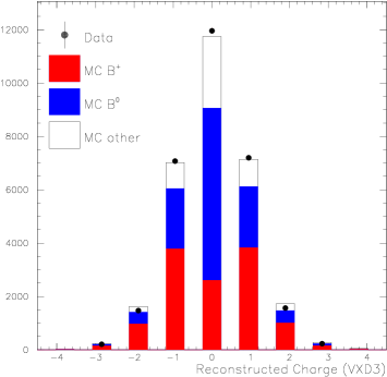
Figure 3: Reconstructed charge, $Q$, for ’97-’98 data and Monte Carlo.

Since the precision of the measurement depends heavily on the charge reconstruction purity, several methods are used to enhance it. In Monte Carlo studies, it was found that the charge reconstruction purity depended on the reconstructed $M_{P_{T}}$, since decays that are missing some tracks tend to have lower $M_{P_{T}}$. Therefore, to enhance the charge purity, events are weighted as a function of $M_{P_{T}}$. For charged decays, the polarized forward-backward asymmetry can be used to tag the $b$ or $\bar{b}$ flavor of the hemisphere. The opposite hemisphere jet charge also provides similar information. If the charge of the decay agrees with that expected from these tags, the decay is weighted more heavily. Conversely, if the charge disagrees, the decay is de-weighted.

The $B^{+}$ and $B^{0}_{d}$ lifetimes are then extracted with a simultaneous binned maximum likelihood fit to the decay length distributions for charged and neutral samples. Figure 4 shows these decay length distributions for data taken in ’97-’98.

For the measurements of $\tau_{B^{+}}$ and $\tau_{B^{0}}$, the dominant systematic error is related to $b$ fragmentation. This is studied by varying both the mean fragmentation energy $<x_{E}>$ and the shape of the $x_{E}$ distribution. The systematic uncertainty from this source is found to be 0.036 ps for both $\tau_{B^{+}}$ and $\tau_{B^{0}}$. For the $\tau_{B^{+}}/\tau_{B^{0}}$ measurement, the uncertainty due to fragmentation largely cancels out, since the two hadrons are assumed to have the same fragmentation function. For this measurement, then, the largest systematics are related to the fraction of $b$-baryons produced ($\Delta(\tau_{B^{+}}/\tau_{B^{0}})=0.013$) and ${\cal B}(B\rightarrow D\bar{D}X)$ ($\Delta(\tau_{B^{+}}/\tau_{B^{0}})=0.011$).

The combined ’93-’98 preliminary results are then

$$\tau_{B^{+}} = 1.686\pm 0.025\pm 0.042\;ps,$$

$$\tau_{B^{0}} = 1.589\pm 0.026\pm 0.055\;ps,$$

$$\tau_{B^{+}}/\tau_{B^{0}} = 1.061\pm^{0.031}_{0.029}\pm 0.027$$

These measurements are the most statistically precise to date and confirm the expectation that the $B^{+}$ and $B^{0}_{d}$ lifetimes are nearly equal.

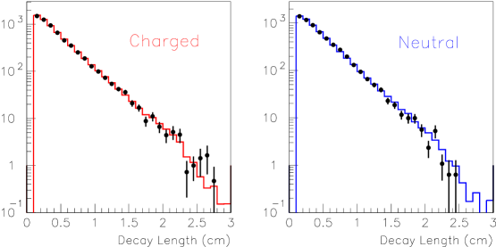
Figure 4: Decay length distributions for charged and neutral samples in ’97-’98 data.

5 Conclusion

We have presented preliminary results on three analyses of $B$ hadron decays. Within the context of the $b\!\rightarrow\!sg$ model described in [12] we find ${\cal B}(\mbox{$b\!\rightarrow\!sg$})<0.076$, at 90% confidence. We have measured ${\cal B}(B\rightarrow D\bar{D}X)$= $(16.2\pm 1.9\pm 4.2)$ %. And, we have measured the lifetimes $\tau_{B^{+}}$, $\tau_{B^{0}}$ with the best statistical precision currently available.

Work is continuing on each of the three analyses. The lifetime analysis will benefit from the addition of 150,000 more $Z^{0}$ decays from the Spring ’98 running. All three analyses will benefit from a re-reconstruction of the data that will incorporate significant tracking improvements. And finally, more SLD running would significantly improve the errors of each of the three analyses.

^∗∗List of Authors

Kenji Abe,⁽²¹⁾ Koya Abe,⁽³³⁾ T. Abe,⁽²⁹⁾ I. Adam,⁽²⁹⁾ T. Akagi,⁽²⁹⁾ N.J. Allen,⁽⁵⁾ W.W. Ash,⁽²⁹⁾ D. Aston,⁽²⁹⁾ K.G. Baird,⁽¹⁷⁾ C. Baltay,⁽⁴⁰⁾ H.R. Band,⁽³⁹⁾ M.B. Barakat,⁽¹⁶⁾ O. Bardon,⁽¹⁹⁾ T.L. Barklow,⁽²⁹⁾ G.L. Bashindzhagyan,⁽²⁰⁾ J.M. Bauer,⁽¹⁸⁾ G. Bellodi,⁽²³⁾ R. Ben-David,⁽⁴⁰⁾ A.C. Benvenuti,⁽³⁾ G.M. Bilei,⁽²⁵⁾ D. Bisello,⁽²⁴⁾ G. Blaylock,⁽¹⁷⁾ J.R. Bogart,⁽²⁹⁾ G.R. Bower,⁽²⁹⁾ J.E. Brau,⁽²²⁾ M. Breidenbach,⁽²⁹⁾ W.M. Bugg,⁽³²⁾ D. Burke,⁽²⁹⁾ T.H. Burnett,⁽³⁸⁾ P.N. Burrows,⁽²³⁾ A. Calcaterra,⁽¹²⁾ D. Calloway,⁽²⁹⁾ B. Camanzi,⁽¹¹⁾ M. Carpinelli,⁽²⁶⁾ R. Cassell,⁽²⁹⁾ R. Castaldi,⁽²⁶⁾ A. Castro,⁽²⁴⁾ M. Cavalli-Sforza,⁽³⁵⁾ A. Chou,⁽²⁹⁾ E. Church,⁽³⁸⁾ H.O. Cohn,⁽³²⁾ J.A. Coller,⁽⁶⁾ M.R. Convery,⁽²⁹⁾ V. Cook,⁽³⁸⁾ R.F. Cowan,⁽¹⁹⁾ D.G. Coyne,⁽³⁵⁾ G. Crawford,⁽²⁹⁾ C.J.S. Damerell,⁽²⁷⁾ M.N. Danielson,⁽⁸⁾ M. Daoudi,⁽²⁹⁾ N. de Groot,⁽⁴⁾ R. Dell’Orso,⁽²⁵⁾ P.J. Dervan,⁽⁵⁾ R. de Sangro,⁽¹²⁾ M. Dima,⁽¹⁰⁾ A. D’Oliveira,⁽⁷⁾ D.N. Dong,⁽¹⁹⁾ M. Doser,⁽²⁹⁾ R. Dubois,⁽²⁹⁾ B.I. Eisenstein,⁽¹³⁾ V. Eschenburg,⁽¹⁸⁾ E. Etzion,⁽³⁹⁾ S. Fahey,⁽⁸⁾ D. Falciai,⁽¹²⁾ C. Fan,⁽⁸⁾ J.P. Fernandez,⁽³⁵⁾ M.J. Fero,⁽¹⁹⁾ K. Flood,⁽¹⁷⁾ R. Frey,⁽²²⁾ J. Gifford,⁽³⁶⁾ T. Gillman,⁽²⁷⁾ G. Gladding,⁽¹³⁾ S. Gonzalez,⁽¹⁹⁾ E.R. Goodman,⁽⁸⁾ E.L. Hart,⁽³²⁾ J.L. Harton,⁽¹⁰⁾ A. Hasan,⁽⁵⁾ K. Hasuko,⁽³³⁾ S.J. Hedges,⁽⁶⁾ S.S. Hertzbach,⁽¹⁷⁾ M.D. Hildreth,⁽²⁹⁾ J. Huber,⁽²²⁾ M.E. Huffer,⁽²⁹⁾ E.W. Hughes,⁽²⁹⁾ X. Huynh,⁽²⁹⁾ H. Hwang,⁽²²⁾ M. Iwasaki,⁽²²⁾ D.J. Jackson,⁽²⁷⁾ P. Jacques,⁽²⁸⁾ J.A. Jaros,⁽²⁹⁾ Z.Y. Jiang,⁽²⁹⁾ A.S. Johnson,⁽²⁹⁾ J.R. Johnson,⁽³⁹⁾ R.A. Johnson,⁽⁷⁾ T. Junk,⁽²⁹⁾ R. Kajikawa,⁽²¹⁾ M. Kalelkar,⁽²⁸⁾ Y. Kamyshkov,⁽³²⁾ H.J. Kang,⁽²⁸⁾ I. Karliner,⁽¹³⁾ H. Kawahara,⁽²⁹⁾ Y.D. Kim,⁽³⁰⁾ M.E. King,⁽²⁹⁾ R. King,⁽²⁹⁾ R.R. Kofler,⁽¹⁷⁾ N.M. Krishna,⁽⁸⁾ R.S. Kroeger,⁽¹⁸⁾ M. Langston,⁽²²⁾ A. Lath,⁽¹⁹⁾ D.W.G. Leith,⁽²⁹⁾ V. Lia,⁽¹⁹⁾ C.Lin,⁽¹⁷⁾ M.X. Liu,⁽⁴⁰⁾ X. Liu,⁽³⁵⁾ M. Loreti,⁽²⁴⁾ A. Lu,⁽³⁴⁾ H.L. Lynch,⁽²⁹⁾ J. Ma,⁽³⁸⁾ G. Mancinelli,⁽²⁸⁾ S. Manly,⁽⁴⁰⁾ G. Mantovani,⁽²⁵⁾ T.W. Markiewicz,⁽²⁹⁾ T. Maruyama,⁽²⁹⁾ H. Masuda,⁽²⁹⁾ E. Mazzucato,⁽¹¹⁾ A.K. McKemey,⁽⁵⁾ B.T. Meadows,⁽⁷⁾ G. Menegatti,⁽¹¹⁾ R. Messner,⁽²⁹⁾ P.M. Mockett,⁽³⁸⁾ K.C. Moffeit,⁽²⁹⁾ T.B. Moore,⁽⁴⁰⁾ M.Morii,⁽²⁹⁾ D. Muller,⁽²⁹⁾ V. Murzin,⁽²⁰⁾ T. Nagamine,⁽³³⁾ S. Narita,⁽³³⁾ U. Nauenberg,⁽⁸⁾ H. Neal,⁽²⁹⁾ M. Nussbaum,⁽⁷⁾ N. Oishi,⁽²¹⁾ D. Onoprienko,⁽³²⁾ L.S. Osborne,⁽¹⁹⁾ R.S. Panvini,⁽³⁷⁾ C.H. Park,⁽³¹⁾ T.J. Pavel,⁽²⁹⁾ I. Peruzzi,⁽¹²⁾ M. Piccolo,⁽¹²⁾ L. Piemontese,⁽¹¹⁾ K.T. Pitts,⁽²²⁾ R.J. Plano,⁽²⁸⁾ R. Prepost,⁽³⁹⁾ C.Y. Prescott,⁽²⁹⁾ G.D. Punkar,⁽²⁹⁾ J. Quigley,⁽¹⁹⁾ B.N. Ratcliff,⁽²⁹⁾ T.W. Reeves,⁽³⁷⁾ J. Reidy,⁽¹⁸⁾ P.L. Reinertsen,⁽³⁵⁾ P.E. Rensing,⁽²⁹⁾ L.S. Rochester,⁽²⁹⁾ P.C. Rowson,⁽⁹⁾ J.J. Russell,⁽²⁹⁾ O.H. Saxton,⁽²⁹⁾ T. Schalk,⁽³⁵⁾ R.H. Schindler,⁽²⁹⁾ B.A. Schumm,⁽³⁵⁾ J. Schwiening,⁽²⁹⁾ S. Sen,⁽⁴⁰⁾ V.V. Serbo,⁽²⁹⁾ M.H. Shaevitz,⁽⁹⁾ J.T. Shank,⁽⁶⁾ G. Shapiro,⁽¹⁵⁾ D.J. Sherden,⁽²⁹⁾ K.D. Shmakov,⁽³²⁾ C. Simopoulos,⁽²⁹⁾ N.B. Sinev,⁽²²⁾ S.R. Smith,⁽²⁹⁾ M.B. Smy,⁽¹⁰⁾ J.A. Snyder,⁽⁴⁰⁾ H. Staengle,⁽¹⁰⁾ A. Stahl,⁽²⁹⁾ P. Stamer,⁽²⁸⁾ H. Steiner,⁽¹⁵⁾ R. Steiner,⁽¹⁾ M.G. Strauss,⁽¹⁷⁾ D. Su,⁽²⁹⁾ F. Suekane,⁽³³⁾ A. Sugiyama,⁽²¹⁾ S. Suzuki,⁽²¹⁾ M. Swartz,⁽¹⁴⁾ A. Szumilo,⁽³⁸⁾ T. Takahashi,⁽²⁹⁾ F.E. Taylor,⁽¹⁹⁾ J. Thom,⁽²⁹⁾ E. Torrence,⁽¹⁹⁾ N.K. Toumbas,⁽²⁹⁾ T. Usher,⁽²⁹⁾ C. Vannini,⁽²⁶⁾ J. Va’vra,⁽²⁹⁾ E. Vella,⁽²⁹⁾ J.P. Venuti,⁽³⁷⁾ R. Verdier,⁽¹⁹⁾ P.G. Verdini,⁽²⁶⁾ D.L. Wagner,⁽⁸⁾ S.R. Wagner,⁽²⁹⁾ A.P. Waite,⁽²⁹⁾ S. Walston,⁽²²⁾ J. Wang,⁽²⁹⁾ S.J. Watts,⁽⁵⁾ A.W. Weidemann,⁽³²⁾ E. R. Weiss,⁽³⁸⁾ J.S. Whitaker,⁽⁶⁾ S.L. White,⁽³²⁾ F.J. Wickens,⁽²⁷⁾ B. Williams,⁽⁸⁾ D.C. Williams,⁽¹⁹⁾ S.H. Williams,⁽²⁹⁾ S. Willocq,⁽¹⁷⁾ R.J. Wilson,⁽¹⁰⁾ W.J. Wisniewski,⁽²⁹⁾ J. L. Wittlin,⁽¹⁷⁾ M. Woods,⁽²⁹⁾ G.B. Word,⁽³⁷⁾ T.R. Wright,⁽³⁹⁾ J. Wyss,⁽²⁴⁾ R.K. Yamamoto,⁽¹⁹⁾ J.M. Yamartino,⁽¹⁹⁾ X. Yang,⁽²²⁾ J. Yashima,⁽³³⁾ S.J. Yellin,⁽³⁴⁾ C.C. Young,⁽²⁹⁾ H. Yuta,⁽²⁾ G. Zapalac,⁽³⁹⁾ R.W. Zdarko,⁽²⁹⁾ J. Zhou.⁽²²⁾

(The SLD Collaboration)

⁽¹⁾Adelphi University, Garden City, New York 11530, ⁽²⁾Aomori University, Aomori , 030 Japan, ⁽³⁾INFN Sezione di Bologna, I-40126, Bologna, Italy, ⁽⁴⁾University of Bristol, Bristol, U.K., ⁽⁵⁾Brunel University, Uxbridge, Middlesex, UB8 3PH United Kingdom, ⁽⁶⁾Boston University, Boston, Massachusetts 02215, ⁽⁷⁾University of Cincinnati, Cincinnati, Ohio 45221, ⁽⁸⁾University of Colorado, Boulder, Colorado 80309, ⁽⁹⁾Columbia University, New York, New York 10533, ⁽¹⁰⁾Colorado State University, Ft. Collins, Colorado 80523, ⁽¹¹⁾INFN Sezione di Ferrara and Universita di Ferrara, I-44100 Ferrara, Italy, ⁽¹²⁾INFN Lab. Nazionali di Frascati, I-00044 Frascati, Italy, ⁽¹³⁾University of Illinois, Urbana, Illinois 61801, ⁽¹⁴⁾Johns Hopkins University, Baltimore, Maryland 21218-2686, ⁽¹⁵⁾Lawrence Berkeley Laboratory, University of California, Berkeley, California 94720, ⁽¹⁶⁾Louisiana Technical University, Ruston,Louisiana 71272, ⁽¹⁷⁾University of Massachusetts, Amherst, Massachusetts 01003, ⁽¹⁸⁾University of Mississippi, University, Mississippi 38677, ⁽¹⁹⁾Massachusetts Institute of Technology, Cambridge, Massachusetts 02139, ⁽²⁰⁾Institute of Nuclear Physics, Moscow State University, 119899, Moscow Russia, ⁽²¹⁾Nagoya University, Chikusa-ku, Nagoya, 464 Japan, ⁽²²⁾University of Oregon, Eugene, Oregon 97403, ⁽²³⁾Oxford University, Oxford, OX1 3RH, United Kingdom, ⁽²⁴⁾INFN Sezione di Padova and Universita di Padova I-35100, Padova, Italy, ⁽²⁵⁾INFN Sezione di Perugia and Universita di Perugia, I-06100 Perugia, Italy, ⁽²⁶⁾INFN Sezione di Pisa and Universita di Pisa, I-56010 Pisa, Italy, ⁽²⁷⁾Rutherford Appleton Laboratory, Chilton, Didcot, Oxon OX11 0QX United Kingdom, ⁽²⁸⁾Rutgers University, Piscataway, New Jersey 08855, ⁽²⁹⁾Stanford Linear Accelerator Center, Stanford University, Stanford, California 94309, ⁽³⁰⁾Sogang University, Seoul, Korea, ⁽³¹⁾Soongsil University, Seoul, Korea 156-743, ⁽³²⁾University of Tennessee, Knoxville, Tennessee 37996, ⁽³³⁾Tohoku University, Sendai 980, Japan, ⁽³⁴⁾University of California at Santa Barbara, Santa Barbara, California 93106, ⁽³⁵⁾University of California at Santa Cruz, Santa Cruz, California 95064, ⁽³⁶⁾University of Victoria, Victoria, British Columbia, Canada V8W 3P6, ⁽³⁷⁾Vanderbilt University, Nashville,Tennessee 37235, ⁽³⁸⁾University of Washington, Seattle, Washington 98105, ⁽³⁹⁾University of Wisconsin, Madison,Wisconsin 53706, ⁽⁴⁰⁾Yale University, New Haven, Connecticut 06511.

References

-
[1]
A.L.Kagan, Phys. Rev. D 51, 6196 (1995);
M. Ciuchini, E. Gabrielli and G. F. Giudice, Phys. Lett. B388, 353 (1996);
B.G. Grzadkowski and W.-S. Hou, Phys. Lett B 272, 383 (1991). - [2] Persis S. Drell in Proceedings of the the XVIII International Symposium on Lepton-Photon Interactions, Hamburg, Germany, July 1997.
- [3] I.I. Bigi, B. Blok, M. Shifman and A. Vainshtein, Phys. Lett B 323, 408 (1994).
- [4] SLD Collaboration, K. Abe et al. Phys. Rev. D 53, 1023 (1996).
- [5] SLD Collaboration, K. Abe et al., Nucl. Instr. & Meth. A400, 287 (1997).
- [6] SLD Collaboration, K. Abe et al., Nucl. Instr. & Meth. A343, 74 (1994).
- [7] SLD Collaboration, K. Abe et al. Phys. Rev. Let. 80, 660 (1998).
- [8] D. Jackson, Nucl. Instr. & Meth. A388, 247 (1997).
- [9] A. Lenz, U. Nierste, and G. Ostermaier, hep-ph/9802202
- [10] SLD Collaboration, Inclusive Search for , SLAC-PUB-7896, July 1998.
- [11] T. Sjöstrand, Comp. Phys. Comm. 82, 74 (1994).
- [12] A. Kagan and J. Rathsmann, hep-ph/9701300
- [13] CLEO Collab.: L. Gibbons et al., Phys. Rev. D 56, 3783 (1997).
- [14] M. Neubert and C.T. Sachrajda, Nucl. Phys. B 483, 339 (1997).
- [15] K. Honscheid, K.R.Schubert and R. Waldi, Z. Phys. C 63, 117 (1994).
- [16] SLD Collaboration, Measurement of the and Lifetimes using Topological Vertexing at SLD, SLAC-PUB-7868, July 1998.