Search for Scalar Top

Abstract

We report results of three searches for scalar top quark. Two of the searches look for direct production of scalar top quark followed by the decay of the scalar quark to charm quark and neutralino or bottom and chargino. The third search looks for top quark decaying to scalar top and neutralino followed by the decay of scalar top to bottom quark and neutralino. We find no evidence for the presence of scalar top quark in any of the searches. Therefore, depending on the search we set limits on the production cross-section, ${\mathcal{B}R}(t\rightarrow\tilde{t}_{1}+\tilde{\chi}_{1}^{0})$, or $m_{\tilde{t}}$ vs. $m_{\tilde{\chi}_{1}^{0}}$.

I Introduction

Supersymmetry (SUSY) assigns to every fermionic SM particle a bosonic superpartner and vice versa [1]. Therefore, the SM quark helicity states $q_{L}$ and $q_{R}$ acquire scalar SUSY partners $\tilde{q_{L}}$ and $\tilde{q_{R}}$ which are also the mass eigenstates for the first two generations to a good approximation. However, a large mixing can occur in the third generation leading to a large splitting between the mass eigenstates [2]. This can lead to a scalar top quark ($\tilde{t}_{1}$) which is not only the lightest scalar quark but also lighter than the top quark.

At the Tevatron, scalar top quark is directly produced in pairs via $gg$ and $q\overline{q}$ fusion diagrams. The cross section depends only on $m_{\tilde{t}}$ at leading order [3]. The dominant next-to-leading order SUSY corrections depend on the other scalar quark masses and are small ($\sim 1\%$). For $m_{\tilde{t}_{1}}$= 110 GeV$/c^{2}$, $\sigma_{\tilde{t}_{1}{\overline{\tilde{t}}}_{1}}$ = 7.4 pb in the next-to-leading order. If $m_{\tilde{t}_{1}}+m_{\tilde{\chi}_{1}^{0}}<m_{t}$, $\tilde{t}_{1}$ can be indirectly produced via the decay $t\rightarrow\tilde{t}_{1}+\tilde{\chi}_{1}^{0}$.

Whenever kinematically allowed, $\tilde{t}_{1}\rightarrow b\tilde{\chi}_{1}^{+}$. If this channel is closed but scalar neutrino ($\tilde{\nu}$) is light, then $\tilde{t}_{1}\rightarrow bl\tilde{\nu}$ dominates. If neither of these channels is allowed, then scalar top decays via a one-loop diagram to charm and a neutralino: $\tilde{t}_{1}\rightarrow c\tilde{\chi}_{1}^{0}$. We assume that $\tilde{\chi}_{1}^{0}$ is the lightest SUSY particle and that R-parity is conserved. Hence the $\tilde{\chi}_{1}^{0}$ is undetected and causes an imbalance of energy.

At CDF, we have performed three separate analyses: (I) direct production of $\tilde{t}_{1}{\overline{\tilde{t}}}_{1}$ with $BR(\tilde{t}_{1}\rightarrow c+\tilde{\chi}_{1}^{0})=100\%$, (II) $t\rightarrow\tilde{t}_{1}\tilde{\chi}_{1}^{0}$ with $\tilde{t}_{1}\rightarrow b\tilde{\chi}_{1}^{+}$, and (III) direct production of $\tilde{t}_{1}{\overline{\tilde{t}}}_{1}$ with $BR(\tilde{t}_{1}\rightarrow b+\tilde{\chi}_{1}^{+})=100\%$.

II Direct search for $\tilde{t}_{1}\rightarrow c\tilde{\chi}_{1}^{0}$

The signature for $\tilde{t}_{1}$ pair production if $\tilde{t}_{1}\rightarrow c\tilde{\chi}_{1}^{0}$ is 2 acolinear charm jets, significant missing transverse energy ($\not\!\!{E}_{T}$), and no high–p_T lepton(s). For this analysis, we have searched data corresponding to a total integrated luminosity of 88$\pm$3.6 pb^-1 collected using the CDF detector during the 1994–95 Tevatron run. CDF is a general purpose detector consisting of tracking, vertexing, calorimeter components and a muon system [4]. Events from this analysis were collected using a trigger which required $\not\!\!{E}_{T}>35$ GeV.

We select events with 2 or 3 jets which have $E_{T}\geq 15$ GeV and $|\eta|\leq 2$ and no other jets with $E_{T}>7$ GeV and $|\eta|<3.6$. The $\not\!\!{E}_{T}$ cut is increased beyond trigger threshold to 40 GeV and we require that $\not\!\!{E}_{T}$ is neither parallel nor anti-parallel to any of the jets in the event to reduce the contribution from the processes where missing energy comes from jet energy mismeasurement: $min\ \Delta\phi(\not\!\!{E}_{T},j)>45^{\circ}$, $\Delta\phi(\not\!\!{E}_{T},j_{1})<165^{\circ}$, and $45^{\circ}<\Delta\phi(j_{1},j_{2})<165^{\circ}$. The jet indices are ordered by decreasing $E_{T}$. We reject events with an identified electron or muon.

To select events with a charm jet, we determine the probability that the ensemble of tracks within a jet is consistent with coming from the primary vertex. We require that at least one jet has a probability of less than 5%.

The largest source of background for this analysis is $W/Z+jets$ production where the vector boson decays to a lepton (e/$\mu$) that is not identified or to a $\tau$ lepton which decays hadronically. There is also a small contribution from Q$CD\ multi$–$jet$ production.

We observe 11 events which is consistent with $14.5\pm 4.2$ events from Standard Model processes. We interpret this as an excluded region in the $m_{\tilde{t}_{1}}$–$m_{\tilde{\chi}_{1}^{0}}$ parameter space as shown in Fig. 1. The maximum $m_{\tilde{t}_{1}}$ excluded is 119 GeV/$c^{2}$ for $m_{\tilde{\chi}_{1}^{0}}=40$ GeV/$c^{2}$.

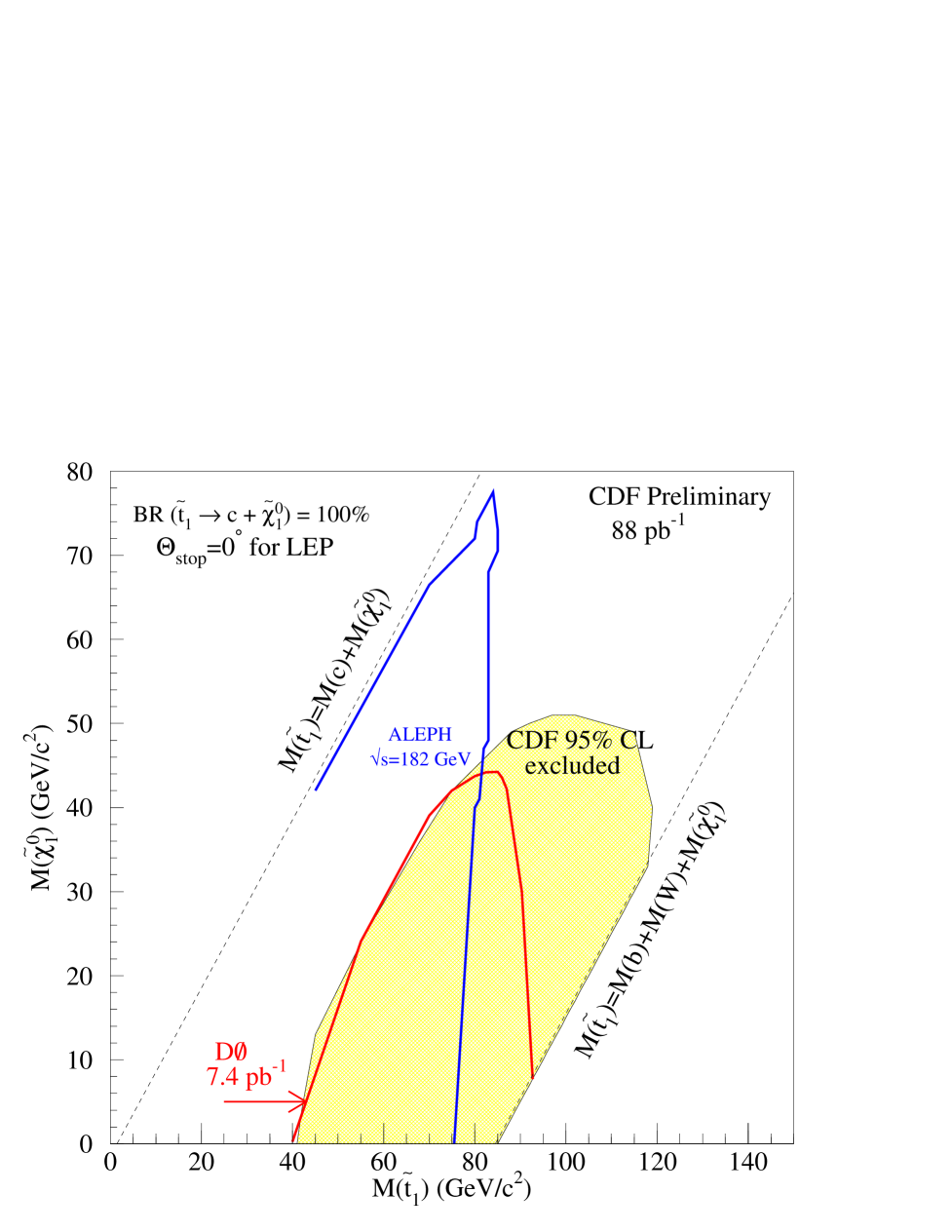
Sample $N_{exp}$ $W^{\pm}(\rightarrow e^{\pm}\nu_{e})+\geq 2$ jets $0.3\pm 0.3\pm 0.1$ $W^{\pm}(\rightarrow\mu^{\pm}\nu_{\mu})+\geq 2$ jets $0.9\pm 0.5\pm 0.3$ $W^{\pm}(\rightarrow\tau^{\pm}\nu_{\tau})+\geq 1$ jets $7.6\pm 1.6\pm 2.2$ $Z^{0}(\rightarrow\nu\overline{\nu})+\geq 2$ jets $1.2\pm 0.4\pm 0.4$ $t\overline{t}$ $0.7\pm 0.2\pm 0.4$ Diboson (WW+WZ+ZZ) $0.4\pm 0.1\pm 0.1$ Total W/Z/Top bkg $11.1\pm 1.8\pm 3.3$ Total QCD bkg $3.4\pm 1.7$ Total Expected $14.5\pm 4.2$ Total Observed $11$ TABLE I.: The expected composition of the data sample after all cuts have been applied.          FIG. 1.: 95% CL limit for $\tilde{t}_{1}\rightarrow c\tilde{\chi}_{1}^{0}$ search. The DØ limits are from [5] and the ALEPH limits are from [6].

III Search for $t\rightarrow\tilde{t}_{1}\tilde{\chi}_{1}^{0}$

If $BR(t\rightarrow\tilde{t}_{1}\tilde{\chi}_{1}^{0})\neq 0$, then top pair production can have three types of events: (1) $t\overline{t}\rightarrow bW^{+}\,\overline{b}W^{-}$ (SM–SM) (2) $t\overline{t}\rightarrow\tilde{t}_{1}\tilde{\chi}_{1}^{0}\,\overline{b}W^{-}$ (SM–SUSY) (3) $t\overline{t}\rightarrow\tilde{t}_{1}\tilde{\chi}_{1}^{0}\,\overline{\tilde{t}}_{1}\tilde{\chi}_{1}^{0}$ (SUSY–SUSY). Further, if $\tilde{t}_{1}\rightarrow b\tilde{\chi}_{1}^{+}$, then all three cases can lead to a signal topology of one isolated, high–p_T lepton (e/$\mu$), three or more high $E_{T}$ jets (one of which is a b jet) and missing transverse energy ($\not\!\!{E}_{T}$). This analysis uses $109.4\pm 7.2$ pb^-1 of inclusive, high–p_T lepton data collected during the 1992–1993 and 1994–1995 Tevatron runs. The cuts used in this analysis are based on the cuts described in [7], [8].

To select events, we start by requiring $\not\!\!{E}_{T}>25$ GeV and a single electron (muon) with $E_{T}(P_{T})>20$ GeV (GeV/c). We reject $Z+jets$ background by looking for an additional lepton of the same flavor but opposite charge and require that the dilepton invariant mass be greater than 105 GeV/c² or less than 75 GeV/c². We also demand that the transverse mass ($M_{T}$) formed by the lepton and the $\not\!\!{E}_{T}$ be greater than 40 GeV/c². The $M_{T}$ cut rejects events where the lepton does not come from the decay of a W (such as Drell-Yan events).

We demand that there be at least three jets with $|\eta|<2$ and the following $E_{T}$ requirements (jets are ordered by decreasing $E_{T}$): $E_{T}$(jet 1) $>20$ GeV, $E_{T}$(jet 2) $>20$ GeV , $E_{T}$(jet 3) $>15$ GeV. We cut on the cosine of the angle between the jet and the proton beam as computed in the rest frame of the event ($\equiv\cos{\theta^{*}_{i}}$). Ordering the three highest $E_{T}$ jets by $|\cos{\theta^{*}_{i}}|$ we demand that $|\cos{\theta^{*}_{i}}|_{1}<0.9,\ |\cos{\theta^{*}_{j}}|_{2}<0.8,\ |\cos{\theta^{*}_{k}}|_{3}<0.7$.

To further reduce the $W+jets$ background, we require that the three highest $E_{T}$ jets are well separated: $\Delta R(j_{i},j_{k})\geq 0.9\ (i,k=1,2,3)$. We also require the transverse momentum of the W (p${}_{T}(W)$), which is constructed from the lepton p_T and $\not\!\!{E}_{T}$, to be large: p${}_{T}(W)>50$ GeV/c. We take advantage of the presence of extra $\tilde{\chi}_{1}^{0}$s in SUSY top events by increasing the $\not\!\!{E}_{T}$ cut: $\not\!\!{E}_{T}>45$ GeV. Finally, we require at least one $b$–jet by demanding at least one SVX–tagged jet [8].

After applying all these selection requirements, our data sample should (as shown from Monte Carlo studies) be composed almost entirely of top events (with both SM and SUSY top decays). For the purposes of setting a limit, we assume that the $W+jets$ background is zero.

To distinguish (SM–SM) events from (SUSY–SM)+(SUSY–SUSY) we exploit the difference in the $E_{T}$(jet 2) and $E_{T}$(jet 3) distributions for these two classes of events. The $E_{T}$(jet 2)/$E_{T}$(jet 3) distributions will be softer for SUSY events relative to SM events. We define a Relative Likelihood ($\equiv\mathcal{R_{L}}$):

$${\mathcal{R_{L}}} = \frac{{\mathcal{L}}_{Abs}^{t\rightarrow\tilde{t}_{1}\tilde{\chi}^{+}}}{{\mathcal{L}}_{Abs}^{t\rightarrow bW^{+}}}$$ (1)

$${\mathcal{L}}_{Abs} = (\frac{1}{\sigma}\frac{d\sigma}{dE_{T}(2)})\times(\frac{1}{\sigma}\frac{d\sigma}{dE_{T}(3)})\ \ \ ({\mathcal{L}}_{Abs}\ {\mathrm{i}s\ derived\ from\ Monte\ Carlo}.)$$ (2)

SM events will have $-\ln{{\mathcal{R_{L}}}}>0$ (SM–like region) and SUSY events will have $-\ln{{\mathcal{R_{L}}}}<0$ (SUSY–like region). This is shown in Fig. 2.

To set a limit on ${\mathcal{B}R}(t\rightarrow\tilde{t}_{1}\tilde{\chi}_{1}^{0})$ as a function of $m_{\tilde{t}_{1}}$,$m_{\chi_{1}^{\pm}}$,$m_{\chi_{1}^{0}}$ we employ the following method. We generate SM top Monte Carlo and SUSY top Monte Carlo for a given ${\mathcal{B}R}$,$m_{\tilde{t}_{1}}$,$m_{\chi_{1}^{\pm}}$,$m_{\chi_{1}^{0}}$. We normalize the sum of SM top and SUSY top in the SM–like region to what is observed in data (9 events). Using this normalization, we can determine the number of SUSY top plus SM top events we expect in the SUSY–like region ($\equiv\mu({\mathcal{B}R})$). We determine the Poisson probability (including errors) that we observe 0 events in the SUSY–like region when we expect $\mu({\mathcal{B}R})$ events and set a 95% Confidence Level (C.L.)  [9] on the ${\mathcal{B}R}$ for a given $m_{\tilde{t}_{1}}$,$m_{\chi_{1}^{\pm}}$,$m_{\chi_{1}^{0}}$. The 95% C.L. on ${\mathcal{B}R}$ as a function of $m_{\tilde{t}_{1}}$,$m_{\chi_{1}^{\pm}}$ for $m_{\chi_{1}^{0}}=40$ GeV/c² is shown if Fig. 3.

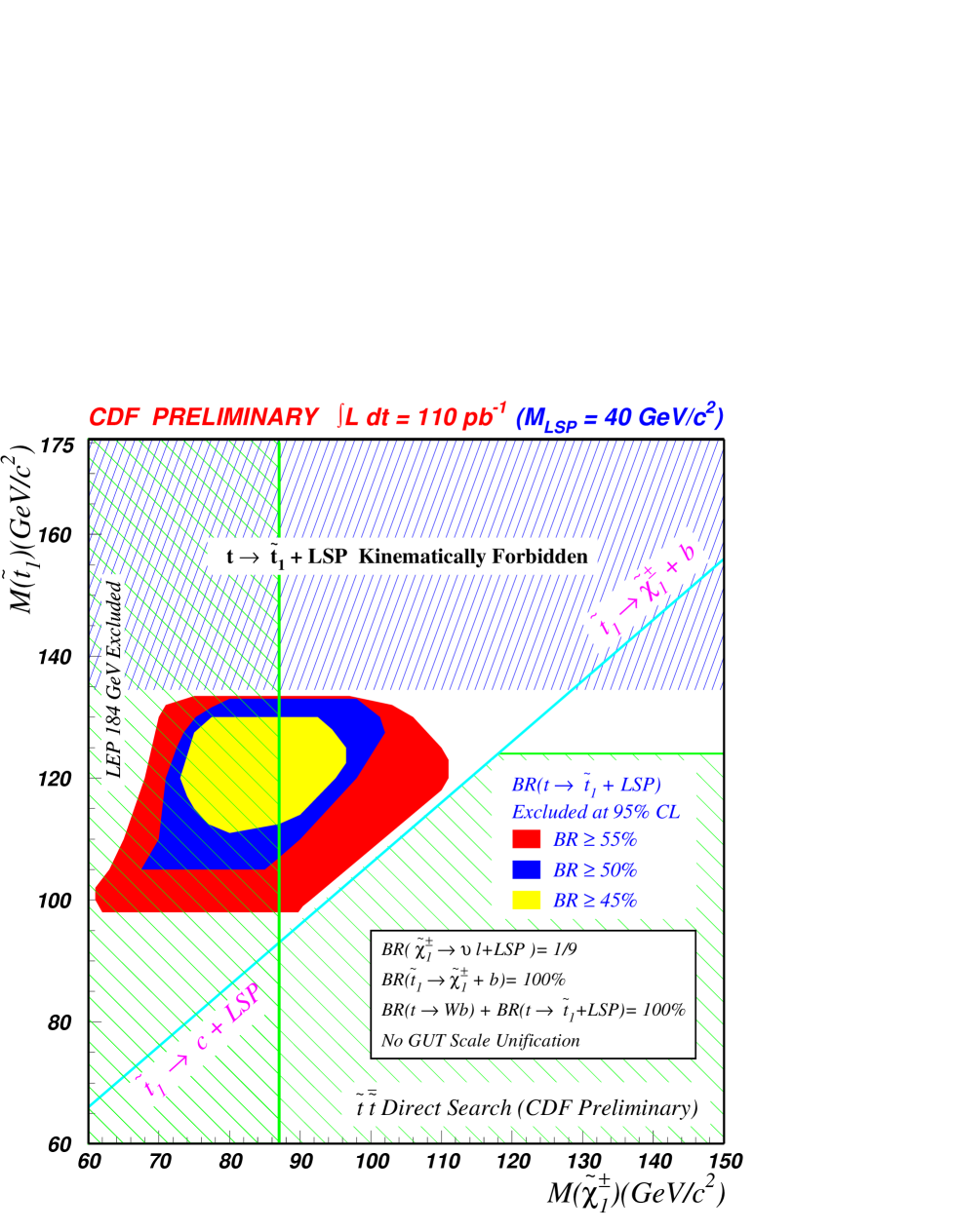
FIG. 2.: The expected $-\log{\mathcal{R}_{L}}$ distribution for top events after all cuts are applied is shown in (a). ${\mathcal{B}R}$($t\rightarrow\tilde{t}_{1}\chi_{1}^{0}$) = 45%. In (b) we overlay the data distribution.          FIG. 3.: The 95% C.L. exclusion contour for $m_{\chi_{1}^{0}}=40$ GeV/c2 and ${\mathcal{B}R}\geq 45,50,55\%$.

IV Direct search for $\tilde{t}_{1}\rightarrow b\tilde{\chi}_{1}^{+}$

If $\tilde{t}_{1}\rightarrow b\tilde{\chi}_{1}^{+}$, then $\tilde{t}_{1}\overline{\tilde{t}}_{1}\rightarrow b\overline{b}\tilde{\chi}_{1}^{+}\tilde{\chi}_{1}^{-}$. We assume that $\tilde{\chi}_{1}^{+}$ is gaugino–like and has the same couplings as the Standard Model W. If one $\chi$ decays leptonically ($\chi^{+}_{1}\rightarrow l\nu\chi^{0}_{1},\ l=e\mu$) and the other $\chi$ decays hadronically ($\chi^{+}_{1}qq^{\prime}\chi^{0}_{1}$) then the final signal topology is one high–p_T lepton (e/$\mu$ only), three or more high–E_T jets (one of which is a $b$–jet), and $\not\!\!{E}_{T}$. We search 90.1$\pm$5.9 pb^-1 of data collected during the 1994–1995 Tevatron run.

To select events, we require one electron (muon) with $E_{T}$ ($P_{T}$) $>20$ GeV (GeV/c) and $\not\!\!{E}_{T}>20$ GeV. We also cut on the jet multiplicity. We demand one jet with $E_{T}>15$ GeV, $|\eta|<2.$, one jet with $E_{T}>8$ GeV, $|\eta|<2.4$ and $\leq 4$ jets with $E_{T}>8$ GeV. After these cuts, we are left with 2249 electron events and 1754 muon events. To make our final sample, we require at least one jet with a SVX tag as defined in Sec. III. Our final sample consists of 47 electron events and 41 muons events.

The data consist of three components: $W+jets$, $t\overline{t}$, and $\tilde{t}_{1}\overline{\tilde{t}}_{1}$. To set a limit on the number of $\tilde{t}_{1}$ events in this sample, we perform an unbinned likelihood fit using two uncorrelated kinematic variables: $M_{T}$ and $\Delta\phi(lepton,j_{2})$ ($j_{2}$ is the second highest $E_{T}$ jet in the event). The likelihood function ($\equiv{\mathcal{L}}$) is:

$${\mathcal{L}}(N_{W},N_{T},N_{S}) = (\prod_{i}\frac{N_{W}W(i)+N_{T}T(i)+N_{S}S(i)}{N_{W}+N_{T}+N_{S}})\cdot\exp{(-(N-N_{obs})^{2}/2N_{obs})}\cdot\exp{(-(N_{T}-\overline{N_{T}})^{2}/2\Delta\overline{N_{T}}^{2})}$$ (3)

The product runs over the number of observed events ($N_{obs}$). $N_{W}/N_{T}/N_{S}$ are the fitted number of $W+jets$/$t\overline{t}$/$\tilde{t}_{1}\overline{\tilde{t}}_{1}$ events and $N=N_{W}+N_{T}+N_{S}$. $W/T/S$ are the joint probability densities for the $M_{T}$ and $\Delta\phi(lepton,j_{2})$ distributions. Since these variables are uncorrelated, the joint probability density is equal to the product of the individual probability densities. For top and $\tilde{t}_{1}$, the probability densities are taken from Monte Carlo after all selection criteria (including SVX tagging) have been applied. For $W+jets$, we use the distributions from data before tagging is applied. The first exponential term constrains, within errors, the total number of events to $N_{obs}$. The second exponential constrains, within errors, the top contribution to what we expect using the theoretical cross–section (5.4$\pm$0.5 pb^-1 [10]).

To set a limit on a given $\tilde{t}_{1}$ mass (for a fixed $m_{\chi^{\pm}_{1}}$,$m_{\chi^{0}_{1}}$), we minimize the negative log likelihood. The minimization returns $N_{S}$ plus its error. Using the total acceptance from Monte Carlo, we convert this into an excluded cross–section. In Fig. 4, we show the $M_{T}$ distribution. The $W+jets$, top, and $\tilde{t}_{1}$ ($m_{\tilde{t}_{1}}=90$ GeV/c²) distributions are normalized to the number of events returned by the $-\log{\mathcal{L}}$ minimization. In Fig. 5 we show the cross-section excluded by data versus the LO cross-section for two pairs of $m_{\chi^{\pm}_{1}}$,$m_{\chi^{0}_{1}}$.

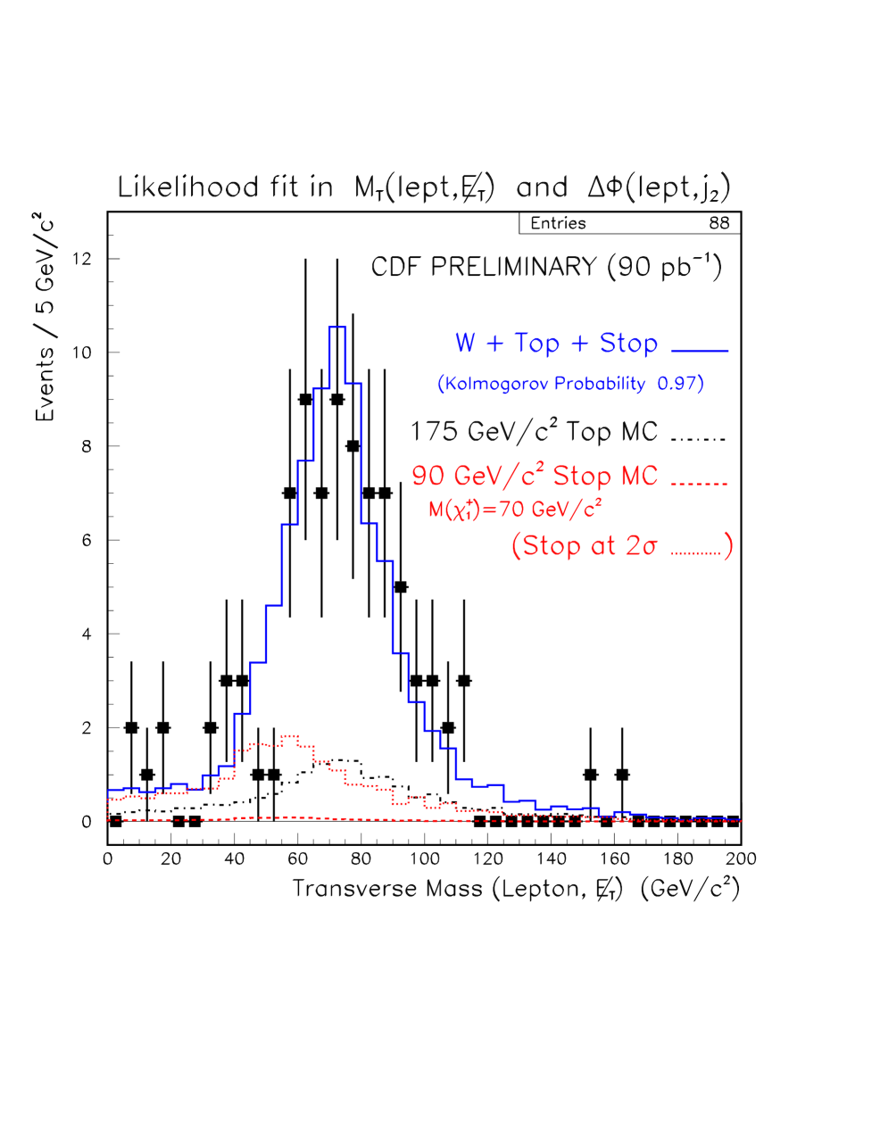
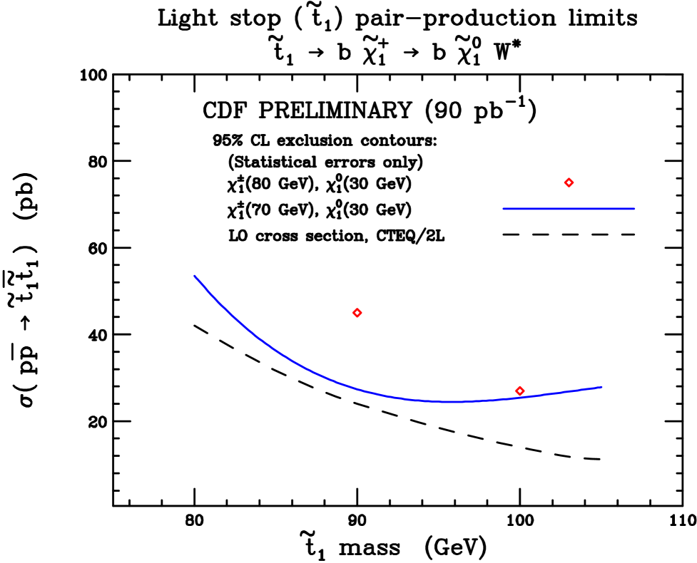
FIG. 4.: $M_{T}$ distribution after tagging. The normalization for the $W+jets$, $t$, and $\tilde{t}_{1}$ distributions is described in the text.          FIG. 5.: The 95% C.L. excluded cross–section as a function of $m_{\tilde{t}_{1}}$ for ($m_{\chi_{1}^{\pm}},m_{\chi_{1}^{0}})$ = (70 GeV/c2,  30 GeV/c2) and (80 GeV/c2,  30 GeV/c2).

V Aknowledgements

We would like to thank Carmine Pagliarone and Michael Gold for their help in understand these analyses. We also thank the Fermilab staff and technical staffs of the participating institutions for their contributions.

REFERENCES

- [1] For reviews of SUSY and the MSSM, see H.P. Nilles, “Supersymmetry, Supergravity And Particle Physics,” Phys. Rept. 110, 1 (1984). H.E. Haber and G.L. Kane, “The Search For Supersymmetry: Probing Physics Beyond The Standard Model,” Phys. Rept. 117, 75 (1985).
- [2] see for example, H. Baer et al., “Phenomenology of light top squarks at the Fermilab Tevatron,” Phys. Rev. D44, 725 (1991). H. Baer, J. Sender and X. Tata, “The Search for top squarks at the Fermilab Tevatron Collider,” Phys. Rev. D50, 4517 (1994).
- [3] W. Beenakker et al., “Stop production at hadron colliders,” Nucl. Phys. B515, 3 (1997).
- [4] F. Abe et al. [CDF Collaboration], “The Cdf Detector: An Overview,” Nucl. Instr. Meth. A271, 387 (1988).
- [5] S. Abachi et al. [D0 Collaboration], “Search for light top squarks in collisions at = 1.8 TeV,” Phys. Rev. Lett. 76, 2222 (1996).
- [6] R. Barate et al. [ALEPH Collaboration], “Scalar quark searches in collisions at = 181 GeV–184 GeV,” Phys. Lett. B434, 189 (1998).
- [7] F. Abe et al. [CDF Collaboration], “Kinematic evidence for top quark pair production in – events in collisions at = 1.8 TeV,” Phys. Rev. D51, 4623 (1995).
- [8] F. Abe et al. [CDF Collaboration], “Observation of top quark production in collisions,” Phys. Rev. Lett. 74, 2626 (1995).
- [9] C. Caso et al., “Review of particle physics. Particle Data Group,” Eur. Phys. J. C3, 1 (1998).
- [10] E.L. Berger and H. Contopanagos, “Top quark production dynamics in QCD,” hep-ph/9512212.