Abstract

The lateral and longitudinal profiles of the hadronic showers detected by iron-scintillator tile hadron calorimeter with longitudinal tile configuration have been investigated. The results are based on $100\ GeV$ pion beam data. Due to the beam scan provided many different beam impact locations with cells it is succeeded to obtain detailed picture of transverse shower behavior. The underlying radial energy densities for four depths and for overall calorimeter have been reconstructed. The three-dimensional hadronic shower parametrisation have been suggested.

1 Introduction

Hadronic shower is a basic notion of hadron calorimetry. But despite that hadronic shower characteristics are studied for many years the exhaustive quantitative understanding of hadronic shower properties is not exist. The published data are as a rule the energy deposition in calorimeter cells and therefore are related with specific cell dimensions and the acceptance of cells relative to shower axis. Furthermore, as to the transverse profiles they are as usual the energy depositions as a function of transverse coordinates, not a radius, and integrated over the other coordinate [1]. Meanwhile for many purposes of experiments a very detailed simulation is not needed and a three dimensional parameterisation of hadron shower development is to become very important for fast simulation which significantly (up to $10^{5}$ times) to speed a detailed GEANT based simulation [2], [3], [5].

In this paper we report on the results of the experimental study of hadronic shower profiles detected by prototype of ATLAS tile hadron calorimeter [6]. This calorimeter has innovative concept of longitudinal segmentation of active and passive layers (see Fig. 1) and the measurement of hadron shower profiles therefore a special interest [7]. This investigation was performed on the basis of data from 100 GeV pion exposure of the prototype calorimeter at the CERN SPS at different $z$ impact points in the range from $-36$ to $20$ cm ($z$ scan) at incident angle $\Theta=10^{o}$ which were obtained in May 1995.

Earlier some results related with lateral shower profiles for this calorimeter were obtained in [8].

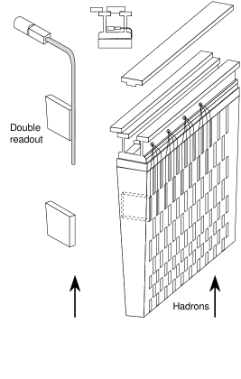
Figure 1: Principle of the tile hadronic calorimeter.

2 The Calorimeter

The prototype the ATLAS hadron tile calorimeter (Fig. 2) is composed of five modules. Each module spans $2\pi/64$ in azimuthal angle, 100 cm in the $z$ direction, 180 cm in the radial direction (about 9 interaction lengths $\lambda_{I}$ at $\eta=0$ or to about 80 effective radiation length $X_{o}$), and has a front face of 100 $\times$ 20 cm² [9]. The iron structure of each module consists of 57 repeated ”periods”. Each period is 18 mm thick and consists of four layers. The first and third layers are formed by large trapezoidal steel plates (master plates), 5 mm thick and spanning the full radial dimension of the module. In the second and fourth layers, smaller trapezoidal steel plates (spacer plates) and scintillator tiles alternate along the radial direction. These layers consist of 18 different trapezoids of steel or scintillator, each spanning 100 mm along $x$ depending on their radial position. The spacer plates and scintillator tiles are 4 mm and 3 mm thick respectively. The iron to scintillator ratio is $4.67:1$ by volume. The calorimeter thickness along $x$ direction at incidence angle $\Theta=10^{o}$ corresponds to 1.49 m of iron equivalent [10].

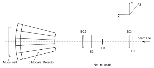
Figure 2: Setup of the tile hadronic calorimeter prototype.

Radially oriented WLS fibers collect light from the tiles at both of their open edges and bring it to photo-multipliers (PMTs) at the periphery of the calorimeter. Each PMT views a specific group of tiles, through the corresponding bundle of fibers. The calorimeter is radially segmented into four depth segments by grouping fibers from different tiles. As a result of each module is divided on 5 (along $z$) $\times$ 4 (along $x$) separate cells.

The readout cells have lateral dimensions of 200 mm (along $z$) $\times$ ($200\div 300$) mm (along $y$, depending from a depth number) and longitudinal dimensions of 300, 400, 500, 600 mm for depths 1-4, corresponding to 1.5, 2, 2.5 and 3 $\lambda_{I}$ at $\eta=0$. On the output we have for each event 200 values of energies $E_{i,j,k,l}$ from $PMT$ properly calibrated [9] with pedestal subtracted. Here indexes i, j, k, l mean: $i=1,\ldots,5$ is the column of cells number (tower), $j=1,\ldots,5$ is the row (module) number, $k=1,\ldots,4$ is the depth number and $l=1,2$ is the $PMT$ number.

The calorimeter has been positioned on a scanning table, able to allow high precision movements along any direction. Upstream of the calorimeter, a trigger counter telescope was installed, defining a beam spot of 2 cm diameter. Two delay-line wire chambers, each with $(z,y)$ readout, allowed to reconstruct the impact point of beam particles on the calorimeter face to better than $\pm$ 1 mm [11]. For the measurements of the hadronic shower longitudinal and lateral leakages backward (80$\times$80 cm²) and side (40$\times$115 cm²) “muon walls” were placed behind and side the calorimeter modules [7].

Construction and performance of ATLAS iron-scintillator barrel hadron prototype calorimeter is described elsewhere [6], [9], [12], [13].

3 The methods for extracting the underlying radial energy density

The incident particle interacts with the material of calorimeter and a shower is initiated. In the following the used coordinate system will be based on the hadron shower direction. The axis of the shower, defined to be a track of a incident particle, forms the $x$ axis with $x=0$ at the calorimeter front face.

We measure the energy depositions in calorimetry cells. In $ijk$-cell of the calorimeter with volume $V_{ijk}$ and cell center coordinates $(x,y,z)$ the energy deposition $E_{ijk}$ is

$$E_{ijk}(x,y,z)=\int\int_{V_{ijk}}\int f(x,y,z)dxdydz,$$ (1)

where f(x,y,z) is the three-dimensional hadron shower energy density function.

In the following we will consider the various marginal (integrated) densities [14]: longitudinal density $f_{1}(x)$ obtained after integrating $f(x,y,z)$ over $y$ and $z$ coordinates

$$f_{1}(x)=\int_{y_{min}}^{y_{max}}\int_{z_{min}}^{z_{max}}f(x,y,z)dydz,$$ (2)

transverse densities $f_{2}(y,z)$ for four depths and overall calorimeter obtained after integrating $f(x,y,z)$ over the various $x$ ranges

$$f_{2}(y,z)=\int_{x_{1}}^{x_{2}}f(x,y,z)dx,$$ (3)

transverse densities $f(z)$

$$f(z)=\int_{x_{1}}^{x_{2}}\int_{-\infty}^{\infty}f(x,y,z)dxdy.$$ (4)

Cumulative function is

$$F(z)=\int_{-\infty}^{z}\int_{-\infty}^{\infty}f_{2}(z,y)dzdy$$ (5)

and related with marginal density $f(z)$ by

$$f(z)=\frac{dF(z)}{dz}.$$ (6)

Due to the azimuthal symmetry densities $f_{2}(y,z)$ are the function only a radius $r=\sqrt{(}y^{2}+z^{2})$ from the shower axis, i.e.

$$f_{2}(y,z)=\Phi(r).$$ (7)

In such case

$$E_{ijk}=\int\int_{V_{ijk}}\Phi(r)rdrd\phi,$$ (8)

where $\phi$ is the azimuthal angle.

There are some methods for extracting of radial density $\Phi(r)$ from the measured distributions of energy depositions $E_{ijk}$.

One method is the unfolding $\Phi(r)$ from (8). This method was used in the analysis of data from the lead-scintillating fiber Spaghetti Calorimeter [15]. Several analytic forms of $\Phi(r)$ were tried, but the simplest that describes the energy deposition in cells was a combination of an exponential and a Gaussian:

$$\Phi(r)=\frac{a_{1}}{r}e^{-\frac{r}{\lambda_{1}}}+\frac{a_{2}}{r}e^{-{(\frac{r}{\lambda_{2}})}^{2}}.$$ (9)

In order to determine the free parameters $a_{i},\lambda_{i}$ in the expression (9) a $\chi^{2}$ minimisation fit have been done.

Another method is using the marginal density function $f(z)$ and its connection with radial density $\Phi(r)$ [16].

$$f(z)=2\int_{|z|}^{\infty}\frac{\Phi(r)rdr}{\sqrt{(}r^{2}-z^{2})}.$$ (10)

This method was used [16] for extracting of electron shower transverse profile on the basis of the data from $GAMS-2000$ electromagnetic calorimeter [17].

Integral equation (10) can be reduced to the Abelian equation by replacing of variables [18]. We solved equation (10) (see Appendix 1) and obtained

$$\Phi(r)=-\frac{1}{\pi}\frac{d}{dr^{2}}\int_{r^{2}}^{\infty}\frac{f(z)dz^{2}}{\sqrt{(}z^{2}-r^{2})}.$$ (11)

The marginal density $f(z)$ also may be determined by various approaches. One approach is the using of cumulative function $f(z)$ [16] and differentiation of it according to (6). Another approach is to assume some form of marginal density $f(z)$, to derive a formula for energy deposition in tower and to determine parameters of $f(z)$ by fitting [19].

If the three exponential distribution for parametrisation of $f(z)$ is used [20], [19]:

$$f(z)=\frac{E_{o}}{2B}\sum_{i=1}^{3}a_{i}e^{-\frac{|z|}{{\lambda}_{i}}},$$ (12)

then for the energy deposition in a tower $E(z)$, the cumulative function $F(z)$, for radial density $\Phi(r)$ we obtain:

$$E(z)=\int_{z-h/2}^{z+h/2}f(z^{\prime}-z)dz^{\prime},$$ (13)

$$E(z)= \frac{E_{o}}{B}\sum_{i=1}^{3}a_{i}{\lambda}_{i}(1-e^{-\frac{h}{2{\lambda}_{i}}}ch(\frac{|z|}{{\lambda}_{i}})), for\ |z|\leq\frac{h}{2},$$ (14)

$$E(z)= \frac{E_{o}}{B}\sum_{i=1}^{3}a_{i}{\lambda}_{i}sh(\frac{h}{2\lambda_{i}})\cdot e^{-\frac{|z|}{{\lambda}_{i}}}, for\ |z|\geq\frac{h}{2},$$ (15)

$$F(z_{r})= \frac{E_{o}}{2B}\sum_{i=1}^{3}a_{i}\lambda_{i}e^{\frac{z_{r}}{\lambda_{i}}}, for\ z_{r}\leq 0,$$ (16)

$$F(z_{r})= \frac{E_{o}}{2}+\frac{E_{o}}{2B}\sum_{i=1}^{3}a_{i}\lambda_{i}(1-e^{-\frac{z_{r}}{\lambda_{i}}}), for\ z_{r}\geq 0,$$ (17)

$$\Phi(r)=\frac{E_{o}}{2B}\sum_{i=1}^{3}\frac{a_{i}}{\pi\lambda_{i}}K_{0}(\frac{r}{\lambda_{i}}),$$ (18)

where $z$ is the transverse coordinate of the tower center, $z_{r}$ is the right edge transverse coordinate of the tower in the center, $h$ is the front face size of towers along $Z$ axis ($h=200\ mm$ in our case), $B=\sum_{i=1}^{3}a_{i}\lambda_{i}$, $E_{o},\ a_{i},\ \lambda_{i}$ are free parameters, $E_{o}$ is an energy normalisation factor, $K_{0}$ is modified Bessel function. Using the condition $\sum_{i=1}^{3}a_{i}=1$ we reduced the number of parameters to six.

The radial containment of shower as a function of $r$ is

$$I(r)=\int_{0}^{r}\int_{0}^{2\pi}\Phi(r)rdrd\phi=\frac{E_{o}}{B}\sum_{i=1}^{3}a_{i}{\lambda}_{i}(1-\frac{r}{{\lambda}_{i}}K_{1}(\frac{r}{{\lambda}_{i}})),$$ (19)

where $K_{1}$ is modified Bessel function.

4 Results

Using the program TILEMON [21] 30 runs with different impact points of incident particles in the range from $-36$ to $20$ cm contained 320 K events have been analysed and the various energy deposition spectra have been obtained.

4.1 Transverse behaviour of hadron showers

4.1.1 Energy deposition in the towers

Figure 3: The energy depositions in towers of 1 $\div$ 4 depths as a function of $Z$ coordinate. Depth 1 — up left, depth 2 — up right, depth 3 — down left, depth 4 — down right. Curves are fits of equation (14) and (15) to the data.

Figure 4: The energy depositions in towers summed overall calorimeter depths as a function of $Z$ coordinate. Curve is the result of fit by formula (14) and (15). Open circles are the Monte Carlo predictions (GEANT-FLUKA+GHEISHA) given in Table 3.

Fig. 3 shows the energy depositions into towers for $1\div 4$ depths as a function of $z$ coordinate of center of tower. Fig. 4 shows the same for overall calorimeter (the sum of histograms presented in Fig. 3). Due to the wide beam scan provided many different beam impact locations with cells and using information from all cells it is succeeded to obtain detailed picture of transverse shower behaviour in calorimeter. The obtained spread of transverse shower dimensions is more than 1000 mm. The energy depositions span a range of three orders of magnitude. It can be seen the flat shoulder at $|z|$ coordinate less than 100 mm. An immediate turnover occur as soon as $|z|$ reached the boundary of the cell. Such picture of transverse shower behaviour was observed in other calorimeters as well [15], [19].

We used these distributions in order to extract the underline marginal density $f(z)$. By adding to statistical errors the electronic noise errors of 27 $MeV$/cell [22], the effective intercalibration error of $2\%$ [9] and uncertainties of $4\%$, arising from the nonzero entry angle of the incident beam into the calorimeter, we obtained a good description of these distributions.

The solid curves in Fig. 3 and 4 are the results of fit with equation (15). In compare with [20], [19], where the transverse profiles exists only for distances less than 250 mm, the our more extended profiles (up to 650 mm) demand to introduce the third exponential.

The parameters $a_{i}$ and $\lambda_{i}$ obtained by fitting are listed in Table 1. As can be seen from Table 1 the slopes of exponentials, $\lambda_{i}$, increase and the contribution of the first exponential, $a_{1}$, decrease as shower develop. The obtained values of $\lambda_{1}$ and $\lambda_{2}$ for overall calorimeter agree well with ones for conventional iron-scintillators calorimeter [20] amount to $18\pm 3$ mm and $57\pm 4$ mm, respectively.

Table 1: The parameters $a_{i}$ and $\lambda_{i}$ obtained by fitting the transverse shower profiles for four depths and overall calorimeter.

	$a_{1}$	$\lambda_{1}$, $mm$	$a_{2}$	$\lambda_{2}$, $mm$	$a_{3}$	$\lambda_{3}$, $mm$
1	$0.88\pm 0.07$	$17\pm 2$	$0.12\pm 0.07$	$48\pm 14$	$0.004\pm 0.002$	$430\pm 240$
2	$0.79\pm 0.06$	$25\pm 2$	$0.20\pm 0.06$	$52\pm 6$	$0.014\pm 0.006$	$220\pm 40$
3	$0.69\pm 0.03$	$32\pm 8$	$0.28\pm 0.03$	$71\pm 13$	$0.029\pm 0.005$	$280\pm 30$
4	$0.41\pm 0.05$	$51\pm 10$	$0.52\pm 0.06$	$73\pm 18$	$0.07\pm 0.03$	$380\pm 140$
all	$0.78\pm 0.08$	$23\pm 1$	$0.20\pm 0.08$	$58\pm 4$	$0.015\pm 0.004$	$290\pm 40$

The shower depth dependences of the parameters $a_{i}$ and $\lambda_{i}$ are displayed in Fig. 5. As can be seen they demonstrated a linear behaviour. The curves are fits of linear equations $a_{i}=\alpha_{i}+\beta_{i}\cdot x$ and $\lambda_{i}=\gamma_{i}+\delta_{i}\cdot x$.

Figure 5: The shower depth dependences of the parameters $a_{i}$ and $\lambda_{i}$.

The values of parameters $\alpha_{i}$, $\beta_{i}$, $\gamma_{i}$ and $\delta_{i}$ are presented in the Table 2. It is interesting that in [1] for the low-density-fine-grained flash chamber calorimeter the linear behaviour of the slope exponential is also observed. In the same time for uranium-scintillator $ZEUS$ calorimeter some non-linear behaviour of slope of halo component measured at 100 $GeV$ has been demonstrated at interaction lengths more then 5 $\lambda$ in shower development [23].

Table 2: The values of parameters $\alpha_{i}$, $\beta_{i}$, $\gamma_{i}$ and $\delta_{i}$.

	$\alpha_{i}$	$\beta_{i}$, $1/\lambda_{\pi}$		$\gamma_{i}$, $mm$	$\delta_{i}$, $mm/\lambda_{\pi}$
$a_{1}$	$0.99\pm 0.06$	$-0.089\pm 0.015$	$\lambda_{1}$	$14\pm 2$	$6\pm 1$
$a_{2}$	$0.04\pm 0.06$	$0.072\pm 0.015$	$\lambda_{2}$	$42\pm 10$	$6\pm 4$
$a_{3}$	$-0.001\pm 0.002$	$0.008\pm 0.002$	$\lambda_{3}$	$170\pm 80$	$30\pm 24$

Table 3 presents the Monte-Carlo predictions for hadron shower energy depositions in the modules of TILECAL at centre coordinates of these modules obtained by using the different hadronic simulation packages interfaced with GEANT [8]. The simulation energy cutoff for neutrons have been set to 1 $MeV$. One can compare our data from Fig. 4 and Monte-Carlo predictions from Table 3 for the same $z$ coordinates. Comparison shows worse agreement, with factor $>3$, at distances of $\pm 400\ mm$ from shower kernel.

Table 3: The average fractions of the energy deposited per module for 100 $GeV$ pions obtained by using the different hadronic simulation packages interfaced with GEANT (G).

Z, mm	$-400$	$-200$	$0$	$200$	$400$
	E, %
G-FLUKA+GHEISHA	$0.43\pm.02$	$4.3\pm.1$	$91\pm 1$	$4.4\pm.1$	$0.43\pm.02$
G-FLUKA+MICAP	$0.20\pm.01$	$3.2\pm.1$	$94\pm 1$	$3.2\pm.1$	$0.18\pm.01$
G-GHEISHA	$0.34\pm.01$	$3.2\pm.1$	$92\pm 1$	$4.5\pm.1$	$0.38\pm.01$

4.1.2 Cumulative function

Similar results were obtained from cumulative function distributions. Cumulative function $F(z)$ was obtained as follows:

$$F(z)=\sum_{k=1}^{4}F^{k}(z),$$ (20)

where $F^{k}(z)$ is the cumulative function for $k$-depth. For each event $F^{k}(z)$ is

$$F^{k}(z)=\sum_{i=1}^{i_{max}}\sum_{j=1}^{5}E_{ijk},$$ (21)

where $i_{max}=1,\ldots,5$ is the last number of tower in sum.

Figure 6: The cumulative functions $F(z)$ for four depths. Depth 1 — up left, depth 2 — up right, depth 3 — down left, depth 4 — down right. Curves are fits of equations (16) and (17) to the data.

Figure 7: Left: The cumulative function $f(z)$ for overall calorimeter. Curves are fits of equations (16) and (17) to the data. Right: The marginal density $f(z)$ for overall calorimeter.

Fig. 6 and 7 (left) present the cumulative functions $F^{k}(z)$ for four depths and for overall calorimeter. The curves are fits of equations (17) to the data. The results of the cumulative function fits are less reliable and in the following we will use the results from energy depositions in tower.

The knowledge of the cumulative function allows us to determine directly according to (6) the marginal density $f(z)$ without additional assumption about its form. This is demonstrated in Fig. 7 (right) where the marginal density $f(z)$ extracted by the numerical differentiation $F(z)$ is shown. Overlayed curve is a calculation of the expression (12) with parameters listed in Table 1. This curve well reproduces the such obtained marginal density.

Thus, the marginal densities $f(z)$ determined by three methods (by using the energy deposition spectrum, the cumulative function and the numerical differentiation of $F(z)$ are in reasonable agreement.

4.1.3 Radial hadron shower energy density

Figure 8: The radial energy density, $\Phi(r)$, as a function of $r$ for TILECAL for various depths: solid lines — the energy densities $\Phi(r)$, dashed lines — the contribution from the first term, dash-dotted lines — the contribution from the second term, dotted lines — the contribution from the third term. Depth 1 — up left, depth 2 — up right, depth 3 — down left, depth 4 — down right.

Figure 9: Left: The radial energy density as a function of $r$ (in units of $\lambda_{f}$) for TILECAL (solid line), the contribution to $\Phi(r)$ from the first term (dashed line), the contribution to $\Phi(r)$ from the second term (dash-dotted line), the contribution to $\Phi(r)$ from the third term (dotted line). Right: The comparison of the radial energy densities as a function of $r$ (in units of $\lambda_{f}$) for TILECAL (solid line) and SPACAL (dash-dotted line).

Fig. 8 and Fig. 9 (left) show the radial shower energy density functions, $\Phi(r)$, calculated by formula (18) with parameters from table 1. The contributions of different terms are also shown. The data of SPACAL calorimeter calculated by formula (9) with ${\lambda}_{1}=140\ mm$ and ${\lambda}_{2}=42.4\ mm$ are shown for comparison on Fig. 9 (right). Since in this work the lateral profiles are presented in term of the measured picocoulombs the density $\Phi(r)$ was transformed into $GeV$ energy scale by using the energy deposit constant of 4 $pC/GeV$ [15].

As can be seen at general reasonable agreement the curve of SPACAL lies systematically below the TILECAL one beyond $1.5\ \lambda_{\pi}^{eff}$.

4.1.4 Radial containment

Figure 10: Left: The containment of shower $I(r)$ (solid line) as a function of radius for overall TILECAL calorimeter. Dash-dotted line — the contribution from first depth, dashed line — the contribution from second depth, thick dotted line — the contribution from third depth, thin dotted line — the contribution from fourth depth. Right: The radii of contained cylinders for given shower containment as a function of depths: black circle – $90\%$ of containment, black square – $95\%$, black triangle – $99\%$. The curves are drawn to guide the eye.

One of the important questions concerns the shower transverse dimensions and its longitudinal development.

The parameterisation of the radial density function, $\Phi(r)$, have been integrated to yield the shower containment as a function of radius, $I(r)$. Fig. 10 (left) shows the transverse containment of the pion shower, $I(r)$, as a function of $r$ for four depths and overall calorimeter.

Table 4: The radii of contained cylinders for given shower containment for TILECAL (for various depths and overall) and SPACAL (overall) calorimeters.

Calorimeter	x in $\lambda_{\pi}^{Fe}$	$r$, in $\lambda_{\pi}^{eff}$
		90 %	95 %	99 %
TILECAL	0.59	0.44	0.64	1.43
	1.97	0.60	0.88	1.55
	3.74	0.92	1.27	1.75
	5.92	1.24	1.55	1.87
	overall	0.72	1.04	1.67
SPACAL	overall	0.86	1.19	1.72

In Table 4 and Fig. 10 (right) the radii of cylinders for given shower containment (90%, 95%, 99%) extracted from Fig. 10 (left) as a function of depth are shown. Solid lines are the linear fit to the data. As can be seen these containment radii increase linearly with the depth. The linear increase of 95depth is also observed for Fe-scintillator calorimeter at 50 and 140 $GeV$ [29]. For overall TILECAL calorimeter the 99% containment radius is equal to $1.7\pm 0.1$ $\lambda_{\pi}^{eff}$. In the last row of this Table the corresponding data for SPACAL calorimeter for 80 $GeV$ $\pi$-mesons are given (a pions grid scan at an angle of $2^{o}$ with respect to fiber direction). Note that in the case of Pb-scintillator calorimeter SPACAL, having the same $\lambda_{\pi}^{eff}$ (see Table 7 in Appendix 2), the shower containment radii are similar to obtained for iron-scintillator calorimeter TILECAL.

It is interesting to note that it is mistaken to consider as the measure of the transverse shower containment the one obtained from the marginal density $f(z)$ or the energy depositions in strips as have been made in [1]. In this work for $99\%$ containment have been obtained the value of $1.2\ \lambda_{I}$ and the conclusion have been made that “their result is consistent with the “rule of thumb” that a shower is contained within a cylinder of radius equal to the interaction length of a calorimeter material [24]”. But it is showed by our and SPACAL measurements that the value of radius of 99% contained shower cylinder amounts to about two interaction length. Reduced value of this radius obtained from $f(z)$ is due to that according to (10) represents the integrated function $\Phi(r)$. In our case if we will use as a measure of shower containment the half-width of integrated $f(z)$ estimated from $F(z)$ in Fig. 7 (left) we obtain the value of $300\ mm$ or $1.2\ \lambda_{\pi}^{eff}$ that agrees with [1].

4.2 Longitudinal Profile

Here we are concerned with the differential deposition of energy $\Delta E/\Delta x$ as a function of $x$, the distance along the shower axis. In Table 5 the average energy shower depositions in various depths, $E_{o}$, the normalised to one interaction length $\lambda_{\pi}^{Fe}$ energy depositions, $\Delta E/\Delta x$, the lengths of depths, $L$, the effective iron lengths of depths, $L_{eff}$, the lengths of depths in units of $\lambda_{\pi}^{Fe}$, the centers of depth intervals in units of $\lambda_{\pi}^{Fe}$, $x$, are given. In these calculations the value of $\lambda_{\pi}^{Fe}=207\ mm$ has been used (see Appendix 3).

Table 5: Average energy shower depositions in various depths.

$x$ in $\lambda_{\pi}^{Fe}$	$\Delta x$ in $\lambda_{\pi}^{Fe}$	$L$, mm	$L_{Fe}$, mm	$E_{o}$, $GeV$	$\Delta E/\Delta x$, $GeV$
0.59	1.18	300	245	25.5$\pm$0.3	21.6$\pm$0.3
1.97	1.58	400	327	43.6$\pm$0.2	27.6$\pm$0.1
3.74	1.97	500	408	22.4$\pm$0.1	11.2$\pm$0.1
5.92	2.37	600	490	8.5$\pm$0.5	3.6$\pm$0.2

In Fig. 11 the our quantities $\Delta E/\Delta x$ (open circle) together with the data of [25] (open triangles) and Monte Carlo predictions ($GEANT-FLUKA+MICAP$, diamonds) [8] are shown. The agreement is observed. So, as to longitudinal energy deposition our calorimeter with longitudinal orientation of the scintillating tiles agrees with the one for a conventional iron-scintillator calorimeters.

Figure 11: Left: Longitudinal profile as a .function of longitudinal coordinate $x$ in units $\lambda_{\pi}^{Fe}$. Open circles are our data, open triangles are conventional calorimeter data, diamonds are the Monte Carlo predictions. Right: The fractions of the “electromagnetic” parts of showers in various depths as a function of $x$.

4.3 “Electromagnetic” fraction of a hadronic shower

The lateral shower profile information may be used for determination of the average fraction of energy going into $\pi^{o}$ production in a hadronic shower, $f_{\pi^{o}}$ [15]. Following [15] we assume that the “electromagnetic” part of hadronic shower is the prominent central core, i.e. in our case the first term. The integrated contribution from this term is $f_{\pi^{o}}=(55\pm 3)\%$. This value may be compared with the one of $56\%$ as simulated by $FLUKA$ for our calorimeter [8], the one of $59\%$ as simulated by $CALOR$ for iron calorimeter [26] and the one of $54\%$ as obtained by using the lead-scintillating fiber $SPACAL$ calorimeter [15].

The observed $\pi^{o}$ fraction, $f_{\pi^{o}}$, is related to the intrinsic actual fraction, $f^{\prime}_{\pi^{o}}$, by the relation [27], [28]:

$$f_{\pi^{o}}=\frac{e/h\cdot f^{\prime}_{\pi^{o}}}{(e/h-1)\cdot f^{\prime}_{\pi^{o}}+1}.$$ (22)

There are two analytic forms for the intrinsic $\pi^{o}$ fraction suggested by Groom [27]

$$f^{\prime}_{\pi^{o}}=1-{(\frac{E}{E_{o}^{\prime}})}^{(m-1)}$$ (23)

and Wigmans [28]

$$f^{\prime}_{\pi^{o}}=k\cdot ln({\frac{E}{E_{o}^{\prime}}}),$$ (24)

where $E_{o}^{\prime}=1\ GeV$, $m=0.85$, $k=0.11$. We calculated the values of $f_{\pi^{o}}$ using a value of $e/h=1.23$ for our calorimeter at $\Theta=10^{o}$ [12] and obtained the values of $f_{\pi^{o}}$ are equal to $55\%$ and $56\%$ for Groom and Wigmans parameterisations of $f^{\prime}_{\pi^{o}}$, respectively. Thus, our measured value of $f_{\pi^{o}}$ agrees well with the experimental one [15] and Monte Carlo calculation [26] and with our calculations.

The determined contributions of parts for various depths give the possibility to obtain the fractions of “electromagnetic” and “hadronic” parts of hadronic showers in various stages of longitudinal development of showers. On the Fig. 11 (right) shows the corresponding results. As can be seen as shower developed the “electromagnetic” fraction decreases. This is natural since the shower energy exhausts and as a result $\pi^{o}$ production decreases. The best fit to these data is $f_{em}=(76\pm 2)-(8.1\pm 0.4)\cdot x$.

5 Conclusions

We have investigated the hadronic shower longitudinal and lateral profiles on the basis of $100\ GeV$ pion beam data at incidence angle $\Theta=10^{o}$ at impact points $Z$ in the range from $-36$ to $20$ cm.

• Some useful formulae for investigating of lateral profiles have been derived:

  • the integral expression (11) for radial density $\Phi(r)$ as a function of marginal density $f(z)$,

  • the formula (18) for radial density $\Phi(r)$ and the formula (16) and (17) for cumulative function $F(z)$ in case of three exponential form of $f(z)$ (12).

• We have obtained for four depths and for overall calorimeter:

  • the energy depositions in towers, $E(z)$;

  • the cumulative functions, $F(z)$;

  • the marginal transversal densities, $f(z)$;

  • the underling radial energy densities, $\Phi(r)$;

  • the containment of a shower as a function of radius, $I(r)$;

  • the radii of cylinders for given shower containment;

  • the fractions of “electromagnetic” part of a shower;

  • the differential longitudinal energy deposition $\Delta E/\Delta x$;

  • the three-dimensional hadronic shower parametrisation.

We have compared our data with relevant data for conventional iron-scintillator calorimeters, SPACAL lead-scintillating fiber calorimeter and Monte Carlo calculations. Our longitudinal profile agree with the ones for a conventional iron-scintillator calorimeters and Monte Carlo prediction. Our lateral profile is not agree with the Monte Carlo prediction.

The three-dimensional hadronic shower parametrization for iron-scintillator calorimeter have been obtained. This parametrisation is important in fast Monte-Carlo simulation for ATLAS calorimetry.

6 Appendix 1.

Solution of Abelian equation.

It is stated above that the marginal density distribution $f(z)$ is connected with the radial energy density $\Phi(r)$ by relation (10). This integral equation can be reduced to the Abelian equation [18]. Here we show how to solve the equation (10) and to obtain the expression (11). Let $\xi=r^{2}$ and $\eta=z^{2}$ so that the equation (10) becomes

$$f(\sqrt{\eta})=\int_{\eta}^{\infty}\frac{\Phi(\sqrt{\xi}),d\xi}{\sqrt{(}\xi-\eta)}.$$ (25)

If we multiply (25) on $\sqrt{\eta-\alpha}$ and obtained product integrate over $d\eta$ in limits $[\alpha,\infty]$ then

$$I=\int_{\alpha}^{\infty}\frac{f(\sqrt{\eta})}{\sqrt{\eta-\alpha}}\,d\eta$$ (26)

Using the following relation

$$\int_{\alpha}^{\infty}d\eta\int_{\eta}^{\infty}d\xi\ldots=\int_{\alpha}^{\infty}d\xi\int_{\alpha}^{\xi}d\eta\ldots$$ (27)

we get

$$I=\int_{0}^{\infty}\Phi(\sqrt{\xi})d\xi\int_{\alpha}^{\xi}\frac{d\eta}{\sqrt{(\xi-\eta)(\eta-\alpha)}}$$ (28)

We should be able to use the fact that

$$\int_{\alpha}^{\xi}\frac{d\eta}{\sqrt{(\xi-\eta)(\eta-\alpha)}}=\pi$$ (29)

and write

$$I=\pi\int_{\alpha}^{\infty}\Phi(\sqrt{\xi})d\xi.$$ (30)

Let us return to former variables $z$, $r$ and $\alpha=r^{2}$. Then (26) and (30) modified into

$${\int}_{r}^{\infty}\frac{zf(z)}{\sqrt{z^{2}-r^{2}}}dz=\pi{\int}_{r}^{\infty}\Phi(r)rdr$$ (31)

Differentiating equation (31) over $r$ we get

$$\Phi(r)=-\frac{1}{\pi}\frac{d}{dr^{2}}\int_{r^{2}}^{\infty}\frac{f(z)dz^{2}}{\sqrt{(}z^{2}-r^{2})}.$$ (32)

7 Appendix 2.

The effective nuclear interaction length, the effective radiation length and the effective Moliere radius.

In reality our calorimeter represents itself the complex structure of various materials and it is necessary to know the effective nuclear interaction length ($\lambda^{eff}$), the effective radiation length ($X_{o}^{eff}$) and the effective Moliere radius ($R_{M}^{eff}$).

We calculated these quantities for our calorimeter. For calculating $\lambda^{eff}$ and $X_{o}^{eff}$ we used the algorithm suggested in [10] so,

$$\lambda^{eff}=\frac{x_{Fe}+x_{Sc}+x_{W}+x_{A}}{x_{Fe}/\lambda_{Fe}+x_{Sc}/\lambda_{Sc}+x_{W}/\lambda_{W}+x_{A}/\lambda_{A}},$$ (33)

where $x_{Fe}$, $x_{Sc}$, $x_{W}$, $x_{A}$ are the volume fractions of the respective materials (Fe, scintillator, wrapping, air) in a period of 18 mm thick of the calorimeter, $\lambda_{i}$ are the corresponding interaction length.

The effective radiation length, $X_{o}^{eff}$, was also calculated by the formula (33) replacing the corresponding $\lambda_{i}$ values by $X_{o,i}$ values. The Moliere radii is equal [14]

$$R_{M}=X_{o}E_{s}/E_{c}$$ (34)

and for a mixture of compound

$$\frac{1}{R_{M}}=\frac{1}{E_{s}}\sum_{j}\frac{x_{j}E_{c}^{j}}{X_{o}^{j}},$$ (35)

where $x_{j}$ are the fraction by weight, $E_{s}=21.2\ MeV$ is the scale energy, $E_{c,j}$ are the critical energy. Critical energy for the chemical elements with the atomic number of $Z$ is equal $E_{c}=610\ MeV/(Z+1.24)$. The values of the $x_{j}$, $\lambda_{j}$ and $X_{o}^{j}$ are given in Table 6

Table 6:

Material	$x_{j}$	$\lambda_{j}$, mm	$X_{o}^{j}$, mm
Fe	14/18	168	17.6
Sc	3/18	795	424
Wrapping	0.2/18	$\lambda_{Sc}$	$X_{o}^{Sc}$
Air	0.8/18	747000	304200

In the Table 7 the results of the our calculations are given. In the fourth column the corresponding values for SPACAL [15] are also shown for comparison. The corresponding values for basic materials of these calorimeters (Fe, Pb) from [14] are also given.

Table 7:

	TILECAL		SPACAL
	eff, mm	Fe, mm	eff, mm	Pb, mm
$X_{o}$	22.4	17.6	7.2	5.6
$R_{M}$	20.5	16.6	20.	16.3
$\lambda_{p}$	206.	168.	210.	171.
$\lambda_{\pi}$	251.	207.	244.	198.

It turns out that the values $\lambda^{eff}$ and $R_{M}^{eff}$ for these two calorimeters are approximately equal. The effective nuclear interaction length for pion was also calculated by using relation $\lambda_{\pi}/\lambda_{p}$ (Appendix 3).

8 Appendix 3.

The nuclear interaction length for pion.

Usually in hadronic calorimetry the nuclear interaction length (${\lambda}_{I}$) given in Review of Particle Physics [14] is used. It is the mean free path for protons between inelastic interactions, calculated using the expression

$${\lambda}_{I}=A/(N_{A}{\sigma}_{I}\rho),$$ (36)

where $A$ is atomic weight, $N_{A}$ is Avogadro number, ${\sigma}_{I}$ is the nuclear inelastic cross section, $\rho$ is a density. For $Fe$ (${\sigma}_{I}=703\ mb$) it amount to 168 mm. But sometimes the pion interaction length is needed as in our case. We calculated the pion and proton interaction lengths and compared with [14] and with the some experimental data [29], [25]. For this we used the absorption cross section of pion and proton on nuclei in the range $60\div 280$ $GeV/c$ measured by [30]. Unfortunately in this work absorption cross section of $\pi$ and $p$ on $Fe$ nuclei are not measured. Therefore we used the nearest cross section for $Cu$ (see Table 8). Transformation from $Cu$ to $Fe$ was performed using the expression

$${\sigma}_{Fe}={\sigma}_{Cu}{(A_{Fe}/A_{Cu})}^{\alpha}.$$ (37)

Table 8: Measured absorption cross sections and parameter $\alpha$ for $Cu$ target.

E	60 GeV		200 GeV
	$\sigma$, mb	$\alpha$	$\sigma$, mb	$\alpha$
$\pi^{+}$	627 $\pm$ 19	0.764 $\pm$ 0.01	629 $\pm$ 19	0.762 $\pm$ 0.01
$p^{+}$	764 $\pm$ 23	0.719 $\pm$ 0.01	774 $\pm$ 23	0.719 $\pm$ 0.01
$\lambda_{\pi}/\lambda_{p}$	$1.22\pm 0.05$		$1.23\pm 0.05$
$\alpha_{p}-\alpha_{\pi}$	$-0.045\pm 0.014$		$-0.043\pm 0.014$

In Table 8 the measured cross sections for $\pi^{+}Cu$ interactions at 60 and 200 $GeV$ together with parameter $\alpha$ are given. Using expressions (36) and (37) cross sections and nuclei interaction lengths are presented in Table 9.

As can be seen from Table 9 the $Fe$ cross sections and nuclear interaction lengths do not depend from energy within errors at $60\div 200$. The mean over energy range values are ${\lambda}_{\pi}=207\pm 7$ mm, ${\lambda}_{p}=168\pm 5$ mm, ${\lambda}_{\pi}/{\lambda}_{p}=1.22\pm 0.05$. The value of ${\lambda}_{p}$ coincides with that given in [14]. The value of ${\lambda}_{\pi}$ may be compared with the measured in [25] value ${\lambda}_{\pi}=200\pm 10$ mm and in [29] value ${\lambda}_{\pi}=190$ mm.

Table 9: Calculated cross sections and nuclei interaction lengths for $Fe$ target.

E	60 GeV	200 GeV
${\sigma}_{\pi}$, mb	568 $\pm$ 18	570 $\pm$ 18
${\sigma}_{p}$, mb	696 $\pm$ 21	705 $\pm$ 23
${\lambda}_{\pi}$, mm	207 $\pm$ 7	207 $\pm$ 7
${\lambda}_{p}$, mm	169 $\pm$ 5	167 $\pm$ 5
${\lambda}_{\pi}/{\lambda}_{p}$	1.22 $\pm$ 0.05	1.24 $\pm$ 0.05

The value measured in [25] presumably have be corrected on iron equivalent length (including scintillators) and then amounts to $210\pm 10$ mm and better agrees with ours.

Using the expressions (36) and (37) we obtained the $A$-dependence of the ratio

$${\lambda}_{\pi}/{\lambda}_{p}(A)={\lambda}_{\pi}/{\lambda}_{p}(Cu){(A/A_{Cu})}^{{\alpha}_{p}-{\alpha}_{\pi}},$$ (38)

where ${\alpha}_{p}-{\alpha}_{\pi}=0.045\pm 0.014$ (Table 8). For $Pb$ nucleus it corresponds to ${\lambda}_{\pi}/{\lambda}_{p}(Pb)=1.16\pm 0.05$. Therefore, it is mistaken to use the value of the ratio ${\lambda}_{\pi}/{\lambda}_{p}(Pb)=1.5$ as have been made in [31] when analysing of data from lead scintillating fiber spaghetti calorimeter.

9 Acknowledgements

This work is the result of the efforts of many people from ATLAS Collaboration. The authors are greatly indebted to all Collaboration for their test beam setup and data taking.

Authors are grateful Peter Jenni for his attention and support of this work. We are indebted to M. Cavalli-Sforza, M. Bosman, I. Efthymiopoulos, A. Henriques, B. Stanek and I. Vichou for the valuable discussions. We are thankful to S. Hellman for the careful reading and constructive advices on the improvement of paper context.

References

- [1] W.J. Womersley et al., NIM A267 (1988) 49.
- [2] R.K. Bock et al., NIM 186 (1981) 533.
- [3] G. Grindhammer et al., NIM A290 (1990) 469.
- [4] A.F. Zarnecki, NIM A339 (1994) 491.
- [5] R. Brun et al., Proceedings of the Second Int. Conf. on Calorimetry in HEP, p. 82, Capri, Italy, 1991.
- [6] ATLAS Collaboration, CERN/LHCC/94-93, ATLAS Technical Proposal for a General-Purpose pp experiment at the Large Hadron Collider CERN, CERN, Geneva, Switzerland.
- [7] M. Lokajicek et al., ATLAS Internal Note, TILECAL-No-63, 1995, CERN, Geneva, Switzerland.
- [8] A. Juste, ATLAS Internal note, TILECAL-No-69, 1995, CERN, Geneva, Switzerland.
- [9] E. Berger et al., CERN/LHCC 95-44, CERN, Geneva, Switzerland.
- [10] M. Lokajicek et al., ATLAS Internal Note, TILECAL-No-64, 1995, CERN, Geneva, Switzerland.
- [11] F. Ariztizabal et al., NIM A349 (1994) 384.
- [12] J.A. Budagov, Y.A. Kulchitsky, V.B. Vinogradov et al., ATLAS Internal Note, TILECAL-No-72, 1996, CERN, Geneva, Switzerland.
- [13] ATLAS TILECAL TDR 3, CERN/LHCC/96-42, 15 December 1996, CERN, Geneva, Switzerland.
- [14] Particle Data Group, Review of Particle Physics, Phys. Rev. D54 (1996) 1.
- [15] D. Acosta et al., NIM A316 (1992) 184.
- [16] A.A. Lednev et al., NIM A366 (1995) 292.
- [17] G.A. Akopdijanov et al., NIM 140 (1977) 441.
- [18] E.T.Whitteker, G.N.Watson, A course of modern analysis. Cambrige, University Press, 1927.
- [19] O.P. Gavrishchuk et al., Preprint JINR, P1-91-554, 1991, Dubna, Russia.
- [20] F. Binon et al., NIM A206 (1983) 373.
- [21] I. Efthymiopoulos, A. Solodkov, The TILECAL Program for Test Beam Data Analysis, User Manual, 1995, CERN, Geneva, Switzerland.
- [22] M. Cobal et al., ATLAS Internal Note, TILECAL-No-67, 1995, CERN, Geneva, Switzerland.
- [23] F. Barreiro et al., NIM A292 (1990) 259.
- [24] U. Amaldi, in Proc. of Int. Conf. on Experimentation at LEP, Uppsala, June 1980 (CERN report EP/80-212, 1980).
- [25] E. Huges, Proceedings of the First Int. Conf. on Calorimetry in HEP, p. 525, FNAL, Batavia, 1990.
- [26] T.A. Gabriel et al., NIM A338 (1994) 336.
- [27] D. Groom, Proceedings of the Workshop on Calorimetry for the Supercollider, Tuscaloosa, Alabama, USA, 1990.
- [28] R. Wigmans, NIM A265 (1988) 273.
- [29] M. Holder et al., NIM 151 (1978) 69.
- [30] A.S. Carroll et al., PL 80B (1979) 319.
- [31] D. Acosta et al., NIM A308 (1991) 481.