HERA Collider Physics

Abstract

HERA, the first electron-proton collider, has been delivering luminosity since 1992. It is the natural extension of an impressive series of fixed-target lepton-nucleon scattering experiments. The increase of a factor ten in center-of-mass energy over that available for fixed-target experiments has allowed the discovery of several important results, such as the large number of slow partons in the proton, and the sizeable diffractive cross section at large $Q^{2}$. Recent data point to a possible deviation from Standard Model expectations at very high $Q^{2}$, highlighting the physics potential of HERA for new effects. The HERA program is currently in a transition period. The first six years of data taking have primarily elucidated the structure of the proton, allowed detailed QCD studies and had a strong impact on the understanding of QCD dynamics. The coming years will bring the era of electroweak studies and high $Q^{2}$ measurements. This is therefore an appropriate juncture at which to review HERA results.

1 Introduction

The ultimate goal of research in high energy physics is to understand and describe the structure of matter and its interactions. The fundamental constituents of matter as we know them today, leptons and quarks, are fermions arranged into generations characterized by lepton numbers and quark flavors, respectively. Leptons are free particles that can be detected. Quarks, on the other hand, only exist in bound states - hadrons. The existence of quarks can be inferred from experimental measurements of the properties of particle interactions and hadron production.

There are four known forces governing our world: gravitational, weak, electromagnetic and strong. Only the last three play a major role in the microscopic world. In the modern language of physics, interactions are due to exchange of field quanta which determine the properties of these interactions. These field quanta correspond to particles whose properties can be measured. All the known carriers of forces are bosons: three vector bosons mediating the weak interactions ($W^{\pm}$, $Z^{0}$), the photon $\gamma$ mediating the electromagnetic interactions and eight gluons $g$ mediating the strong interactions. Each of them carries specific quantum numbers, as do the fundamental constituents of matter.

There is no theory limiting the number of generations. The only theoretical condition is that the number of lepton generations be equal to that of the quarks. At present three generations of leptons and quarks are known. The leptons are the electron – $e$, the muon – $\mu$ and the tau – $\tau$, each one accompanied by a corresponding neutrino, $\nu_{e}$, $\nu_{\mu}$ and $\nu_{\tau}$. There are six known quarks, the up – $u$, down – $d$, strange – $s$, charm – $c$, bottom – $b$ and top – $t$ quarks. Neutrinos, which carry no electric charge, interact only weakly. Charged leptons take part in weak and electromagnetic interactions. Only quarks take part in all the known interactions of the micro-world.

The theoretical framework which allows us to describe formally this simple picture is based on gauge theories. The weak and electromagnetic interactions are unified within the so-called electroweak theory formulated by Glashow, Salam and Weinberg (?; ?; ?). The strong interactions are embedded in the framework of Quantum Chromodynamics (?). The combination of the two constitutes what is generally known as the Standard Model of particles and interactions. The experimental evidence which led to this simple and elegant picture has been provided by a multitude of experiments involving high energy interactions of hadrons with hadrons, leptons with hadrons, and leptons with leptons.

The description of electroweak interactions is based on the SU(2) group of weak isospin and U(1) group of weak hyper-charge. This symmetry is spontaneously broken at $\sim 100$ GeV by introducing in the theory scalar mesons called Higgs particles. In the resulting theory we find two charged and one neutral massive vector bosons – the $W^{\pm}$ and the $Z^{0}$, which mediate weak interactions, and one massless neutral vector boson – the photon. While the existence of the weak charged currents was known (since the explanation of the $\beta$ decay of atomic nuclei by Fermi in 1932), this theory predicted the existence of weak neutral currents, which were subsequently discovered (?).

The experimental and theoretical progress achieved in the electroweak sector is tremendous. The $W^{\pm}$ and the $Z^{0}$ were discovered at the CERN proton-antiproton collider (?; ?) and with the advent of two high energy electron positron colliders, LEP and SLC, the electroweak parameters of the Standard Model have been determined to a high precision (?; ?). Suffice to say that the experiment and the theory agree with each other at the level of ${\mathcal{O}}(10^{-3})$ (?). The Higgs boson remains the only missing link. Global fits constrain the Higgs mass at $95\%$ confidence level to be $m_{H}<500$ GeV (?), with the minimum $\chi^{2}$ corresponding to a value $m_{H}\simeq 115$ GeV.

The interactions of quarks and gluons are described by Quantum Chromodynamics (QCD), a non-abelian gauge theory based on the SU(3) color symmetry group. Color constitutes the equivalent of the electric charge in electromagnetic interactions. The quarks, each in three colors, interact by exchange of electrically neutral vector bosons - the gluons, which form a color charge octet. The gluons are not color neutral and thus they themselves interact strongly. A consequence of this property is asymptotic freedom which states that the interaction strength of two colored objects decreases the shorter the distance between them. The effective strong coupling constant $\alpha_{s}$ depends on the scale at which the QCD process occurs. The solution of the renormalization group equation in leading order leads to

$$\alpha_{s}(Q^{2})=\frac{4\pi}{\beta_{0}\ln(Q^{2}/\Lambda^{2})}\ ,$$ (1)

where $Q^{2}$ denotes the scale at which $\alpha_{s}$ is probed and $\Lambda$ is a QCD cut-off parameter. The parameter $\beta_{0}$ depends on the number of quark flavors in the theory, $N_{f}$,

$$\beta_{0}=11-\frac{2}{3}N_{f}\ .$$ (2)

Since the known number of flavors is six, $\beta_{0}>0$, and the coupling constant becomes smaller the larger the scale $Q^{2}$. The property of asymptotic freedom has been proven rigorously and allows to make predictions for the properties of strong interactions in the perturbative QCD regime, in which $\alpha_{s}$ is small.

Another property of QCD, which has not been proven rigorously, is confinement, which keeps quarks bound into colorless hadrons and prevents the observations of free quarks. In QCD, the color degree of freedom and confinement explain why the observed hadrons are made either of $q\bar{q}$ or of $qqq$ ($\bar{q}\bar{q}\bar{q}$) states. These combinations ensure that hadrons are colorless and have integer electrical charge. It also explains why baryons made out of three quark states are fermions while mesons made out of $q\bar{q}$ states are bosons (?). The model in which hadrons are viewed as composed of free quarks $q$ or antiquarks $\bar{q}$ is called the Quark Parton Model (QPM). In the presence of QCD, the naive QPM picture of hadrons has to be altered to take into account the radiation and absorption of gluons by quarks as well as the creation of $q\bar{q}$ pairs by gluons. Thus in effect hadrons consist of various partons, quarks and gluons. We know today that about 50% of the proton momentum is carried by gluons.

QCD has two properties which make it much more difficult to work with theoretically than electroweak theory. The first poperty is that the coupling constant is large, making the use of perturbation theory difficult. The strong coupling constant depends on the scale, as described above, and cross sections can only be calculated for scatterings with a hard scale, for which $\alpha_{s}$ is small enough. The second property is the non-Abelian nature of the interaction. Gluons can interact with other gluons, leading to confinement of color.

The distribution of partons bound in hadrons cannot be calculated from first principles. The calculations would have to be performed in a regime of QCD where the perturbative approach breaks down. However the QCD factorization theorem (?) states that for hard scattering reactions the cross section can be decomposed into the flux of universal incoming partons and the cross section for the hard subprocess between partons. The measurement of parton distributions in hadrons becomes an essential element in testing the validity of QCD.

QCD has been tested in depth in the perturbative regime and describes the measurements very well. However, because the observables are based on hadron states rather than the partonic states to which perturbative calculations apply the precision level which is achieved in testing QCD is lower than in case of the electroweak interactions. In addition, up to now there is no understanding within QCD of scattering processes in the non-perturbative regime, the so called soft regime, although this is the regime which dominates the cross section for strong interactions.

The soft hadron-hadron interactions are well described by the Regge phenomenology (?) in which the interaction is viewed as due to exchanges of collective states called Regge poles. The Regge poles can be classified into different families according to their quantum numbers. Among all possible families of Regge poles there is a special one, with the quantum numbers of the vacuum, called the pomeron ($I\!\!P$) trajectory. The pomeron trajectory is believed to determine the high energy properties of hadron-hadron interaction cross sections. The link between Regge theory and QCD has not yet been established.

QCD remains a largely unsolved theory and the justification for the use of perturbative QCD rests to a large extent directly on experiment. Every experiment in strong interactions involves a large range of scales, over which the value of the strong coupling constant changes radically. This, together with certain arbitrariness in truncating the perturbative expansion, leads to uncertainties which can only be successfully resolved if the gap between the perturbative and non-perturbative approach is bridged.

The advantage of lepton-nucleon collisions in studying the structure of matter lies in that leptons are point-like objects and their interactions are well understood. The point-like, partonic substructure of the nucleon was first firmly established in the pioneering SLAC experiment (?; ?) in which the spectrum of electrons scattered off a nucleon target was measured. This experiment was very similar in its essence to the famous Rutherford experiment which established the structure of atoms. In a scattering in which an electron of initial four momentum $k$ emerges with four momentum $k^{\prime}$, the exchanged virtual photon has a mass $q^{2}=(k-k^{\prime})^{2}=-Q^{2}$ and correspondingly a Compton wavelength of $\hbar/\sqrt{Q^{2}}$. Thus for different values of $Q^{2}$ the interaction is sensitive to structures at different scales.

The picture that has emerged from measurements of lepton-nucleon scattering, in particular from deep inelastic scattering (DIS), utilizing electron, muon and neutrino beams, confirmed the universality of parton distributions as well as the validity of perturbative QCD which predicts a change in the observed parton distributions as a function of the scale at which they are probed (for a review see ?).

Charged lepton-nucleon interactions also are an ideal laboratory to study photon-nucleon interactions. When the lepton scattering angle is very small the exchanged photon is almost real and the leptons can be thought of as a source of photons that subsequently interact with the nucleon. At high photon energies we can then study the properties of photon interactions with hadronic matter. A simple guess would be that photons, as gauge particles mediating electromagnetic interactions, would interact only electromagnetically. However, given the Heisenberg uncertainty principle, the photon can fluctuate into a quark-antiquark pair, which can then develop further structure. In the presence of a hadronic target, the interaction can then be viewed as hadron-hadron scattering.

In many respects the HERA accelerator, in which 27.5 GeV electrons or positrons collide with 820 GeV protons, offers a unique possibility to test both the static and dynamic properties of the Standard Model. The center-of-mass energy of the electron-proton collisions is 300 GeV and is more than a factor 10 larger than any previous fixed target experiment. The available $Q^{2}$ range extends from $Q^{2}\simeq 0$ to $Q^{2}\simeq 9\cdot 10^{4}$ GeV² and allows to probe structures down to $10^{-16}$ cm, while partons can be probed down to very small fractions of the proton momentum, $x=Q^{2}/(Q^{2}+W^{2})\sim 10^{-5}$. Two general purpose experiments, H1 and ZEUS, are dedicated to the study of the HERA physics.

The first 0.02 pb^-1 of luminosity delivered by the HERA accelerator has brought striking results which have opened a whole new interest in QCD. In the deep inelastic regime, $Q^{2}\geq 10$ GeV², in which the partons can be easily resolved, it was found that the number of slow partons increases steadily with decreasing $x$ (?; ?). This observation is in line with asymptotic expectations of perturbative QCD. Further studies have shown that an increase is observed even at $Q^{2}$ as low as 1 GeV (?), where it is not even clear that the parton language is applicable. It was also found that a large fraction of DIS events had a final state typical of diffractive scattering always believed to be a soft phenomenon (?; ?). This opened the interesting possibility to explore the partonic nature of the pomeron and provide some link between the Regge theory and QCD.

Before the advent of HERA the complicated nature of the photon was inferred from low energy photon hadron interactions where the photon behaved essentially as a vector meson, a bound state of a $q\bar{q}$ (?). On the other hand in $\gamma\gamma$ interactions derived from $e^{+}e^{-}$ interactions, the photon behaved as if it consisted mainly of $q\bar{q}$ states which could be calculated in perturbative QCD (?). The missing link was established at TRISTAN (?) and at HERA (?; ?). The cross section for photon induced jet production could not be explained without a substantial contribution from a photon consisting of partons. The presence of the photon remnant after the hard collision was observed for the first time with the HERA detectors (?; ?).

The investigation of hadronic final states in DIS and hard photoproduction scattering demonstrated that we still do not have a complete understanding of the transition from partonic states to the hadronic ones in the region affected by proton fragments (?; ?). This is unlike the description of the hadronic final states produced in $e^{+}e^{-}$ interactions where models tuned to describe low energy interactions hold very well in the increased phase space (?). Here again the message is that simple quark parton model approaches corrected for perturbative QCD effects are not adequate when one of the initial particles has by itself a complicated nature.

At very large $Q^{2}>1000\,\mathrm{GeV^{2}}$, where the contribution of $W$ and $Z^{0}$ exchanges become important, the measured cross sections are generally well described by the Standard Model. However, an excess of events was reported in the region of large $x>0.4$ and very high $Q^{2}>15000\,\mathrm{GeV^{2}}$ by both the H1 and the ZEUS experiment (?; ?). The origin of these is not yet understood, but the presence of these events underscores the discovery potential at HERA for new physics beyond the Standard Model.

In the following chapters, we review HERA physics in some depth. More detailed discussion of some aspects of HERA physics can be found in recent reviews (?; ?; ?; ?) as well as in selected lecture notes (?; ?).

2 Lepton-nucleon scattering

The HERA physics program to date has primarily focused on testing our understanding of the strong force. Measurements have been performed in kinematic regions where perturbative QCD calculations should be accurate, as well as in regions where no hard scale is present and non-perturbative processes dominate. In the following sections, we introduce the language of structure functions and the effects expected from pQCD evolution. This background serves as the base for interpreting many of the physics results described in later sections.

Fig. 1: Schematic diagram describing deep inelastic lepton nucleon scattering. The four vectors of the particles, or particles systems, are given in parantheses.

In the most general case the lepton-nucleon interaction proceeds via the exchange of a virtual vector boson as depicted in Fig. 1. Since the lepton number has to be conserved, we expect the presence of a scattered lepton in the final state, while the nucleon fragments into a hadronic final state $X$,

$$lN\to l^{\prime}X\ .$$ (3)

Assuming that $k$, $k^{\prime}$, $P$, $P^{\prime}$ are the four vectors of the initial and final lepton, of the incoming nucleon and of the outgoing hadronic system, respectively (see Fig. 1), the usual variables describing the lepton nucleon scattering are

$$Q^{2} = -q^{2}=-(k-k^{\prime})^{2}\ ,$$

$$s = (k+P)^{2}\ ,$$

$$W^{2} = (q+P)^{2}=p_{\prime}^{2}\ ,$$

$$x = \frac{Q^{2}}{2P\cdot q}\ ,$$ (4)

$$y = \frac{q\cdot P}{k\cdot P}\ ,$$

$$\nu = \frac{q\cdot P}{m_{N}}\ .$$

The variables $s$ and $W^{2}$ are the center-of-mass energy squared of the lepton-nucleon and intermediate boson-nucleon systems, respectively. The square of the four momentum transfer (the mass squared of the virtual boson), $q^{2}<0$, determines the hardness of the interaction, or in other words, the resolving power of the interaction. The exchanged boson plays the role of a “partonometer” with a resolution $\Delta b$,

$$\Delta b\sim\frac{\hbar c}{\sqrt{Q^{2}}}=\frac{0.197}{\sqrt{Q^{2}}}\,\mbox{\rm GeV fm}\ ,$$ (5)

where for convenience we introduce the positive variable $Q^{2}=-q^{2}$. The meaning of $\nu$ and $y$ is best understood in the rest frame of the target, in which $\nu$ is just the energy of the intermediate boson and $y$ measures the inelasticity of the interaction and its distribution reflects the spin structure of the interaction. The variable $x$ is the dimensionless variable introduced by Bjorken.

Fig. 2: An example of the electron spectrum measured in electron proton scattering. From right to left, the direction of increasing inelasticity, $y$, we first observe a peak which corresponds to an elastic $ep\rightarrow ep$ interaction (?), then a series of maxima which correspond to the proton excited states and then a continuum (?).

Fig. 3: The inelastic $ep\rightarrow eX$ cross section scaled by the Mott cross section for fixed $W$ values as a function of $Q^{2}$ as measured in the SLAC experiment (?). For comparison the elastic $ep\rightarrow ep$ cross section with dipole formfactors scaled by the Mott cross section is shown for electron scattering angle $\theta=10^{o}$ (dotted dashed line). The lines connecting the data points are to guide the eye (adapted from Fig. 1 of ?).

By selecting the outgoing lepton energy and angle we can vary the values of $Q^{2}$ and $y$, thus probing the charge distribution (electromagnetic or weak) within the nucleon. An example of the scattered electron energy, $E^{\prime}$, spectrum as measured in electron proton collisions (?) is shown in Fig. 2. From right to left, the direction of increasing inelasticity $y$, we first observe a peak which corresponds to an elastic $ep\rightarrow ep$ interaction in which the proton remains intact (?). We then observe a series of maxima which correspond to the proton excited states and then a continuum. Should the charge distribution in the proton be continuous we would expect, in the region of continuum, a decrease of the cross section with increasing $Q^{2}$ following the Rutherford formula. The experimentally observed spectrum turned out to be much flatter (see Fig. 3). This was the first indication that there is a substructure inside the nucleon.

The derivation of the formula for the inclusive scattering cross section (which is beyond the scope of this review) is very similar to that of $e\mu$ scattering. The unknown couplings of the lepton current to the nucleon are absorbed in the definition of the structure functions, $F_{i}$, which can be thought of as Fourier transforms of the spatial “charge” distribution.

The inclusive differential cross section, integrated over all possible hadronic final states, is a function of two variables which uniquely determine the kinematics of the events. These variables are most easily recognizable as the energy and production angle of the scattered lepton. However, in anticipation of the partonic structure of hadrons, the differential cross section is usually expressed in terms of two variables, $x$ and $Q^{2}$, defined in Eq. (2),

$$\frac{d^{2}\sigma^{l(\bar{l})N}}{dxdQ^{2}}=A\left\{\frac{y^{2}}{2}2xF_{1}(x,Q^{2})+(1-y)F_{2}(x,Q^{2})\pm(y-\frac{y^{2}}{2})xF_{3}(x,Q^{2})\right\}\ ,$$ (6)

where, for $Q^{2}\ll M^{2}_{W,Z}$ (the mass squared of the intermediate vector bosons), $A=G_{F}^{2}/2\pi x$ for neutrinos and anti-neutrinos with $G_{F}$ the Fermi constant, and $A=4\pi\alpha^{2}/xQ^{4}$ for charged leptons with $\alpha$ the electromagnetic coupling constant.

The structure functions, $F_{i}$, may depend on the kinematics of the scattering and the chosen variables are $x$ and $Q^{2}$. The reason for this choice will become clearer in the next sections. The structure functions, $F_{1}$, $F_{2},$ and $F_{3}$ are process dependent. The $F_{3}$ structure function is non-zero only for weak interactions and is generated by the parity violating interactions. In the following, after discussing the kinematics of lepton-nucleon scattering, we will concentrate on the interpretation and properties of the structure functions.

2.1 Kinematics of lepton-nucleon scattering

The variables used in describing the properties of lepton-nucleon scattering are defined by Eq.( 2). Here we would like to discuss in more detail their meaning. We will do so assuming that the mass of the incoming and scattered leptons are negligible and, in preparation for the HERA conditions, that the nucleon is a proton with mass $m_{p}$.

The variable $s=(p+k)^{2}\simeq m_{p}^{2}+2p\cdot k$ is the square of the center-of-mass energy. However, an energy variable which is more appropriate at HERA is $W$, which is the invariant mass of the system recoiling against the scattered lepton and can be interpreted as the center-of-mass energy of the virtual boson-proton system.

$$W^{2}=(P+q)^{2}=m_{p}^{2}-Q^{2}+2P\cdot q=ys-Q^{2}+m_{p}^{2}(1-y)\ ,$$ (7)

where in the last step we have used the definition of $y$ (see Eq. (2)). The variable $y$ is an invariant and in the proton rest frame the expression for $y$ reduces to

$$y=1-\frac{E^{\prime}_{l}}{E_{l}}\,,$$ (8)

where $E_{l}$, $E^{\prime}_{l}$ are the energies of the incoming and scattered lepton in this frame, respectively. It is easy now to infer the most general limits on $y$,

$$0\leq y\leq 1\,.$$ (9)

The variable $y$ is a measure of the fraction of the energy from the electron transferred to the interaction. The limits on $x$ can be readily deduced from the following:

$$x=\frac{Q^{2}}{2P\cdot q}=\frac{Q2}{W^{2}+Q^{2}-m_{p}^{2}}\ ,$$ (10)

where we have used the relation (7) in the last step. Since $Q^{2}\geq 0$ and $W^{2}$ cannot be smaller than $m_{p}^{2}$ the upper limit on $x$ is $x\leq 1$. In practice the lower limit is determined by the maximum $W^{2}$ available in the interaction, but formally $x$ can be infinitely small, although positive. Thus,

$$0\leq x\leq 1\ .$$ (11)

The interpretation of $x$ is easiest in the QPM language. Define $z$ as the fraction of the proton momentum carried by the struck quark and $p^{\prime}$ is the four momentum of the outgoing quark. If we assume that the quark masses are zero as dictated by QPM (i.e. $(zP)^{2}=p^{\prime 2}=0$) then

$$p^{\prime 2}=(zP+q)^{2}=2zP\cdot q-Q^{2}=0\,.$$ (12)

It can be readily seen that $z=x$. Thus in the QPM $x$ is the fraction of the proton momentum carried by the struck massless quark. Note also that for $Q^{2}\ll W^{2}$,

$$x\simeq\frac{Q^{2}}{W^{2}}\,,$$ (13)

and for fixed values of $Q^{2}$, the higher the $W$ the lower the $x$.

The value of $Q^{2}$ depends only on the lepton vertex and is given by

$$Q^{2}=2E_{l}E^{\prime}_{l}(1-\cos\theta)\,$$ (14)

where $\theta$ is the angle between the initial and scattered lepton. This expression is valid in all frames of reference. The larger the scattering angle and the larger the energy of the scattered lepton, the larger the $Q^{2}$. The maximum $Q^{2}$ is limited by $s$,

$$Q^{2}=xy(s-m_{p}^{2})\,,$$ (15)

and occurs when both $x$ and $y$ tend to one. For a given $Q^{2}$ the lowest $x$ is achieved when $y=1$ and the lowest $y$ when $x=1$. Thus kinematically the small values of $x$ are associated with large values of $y$ and vice versa.

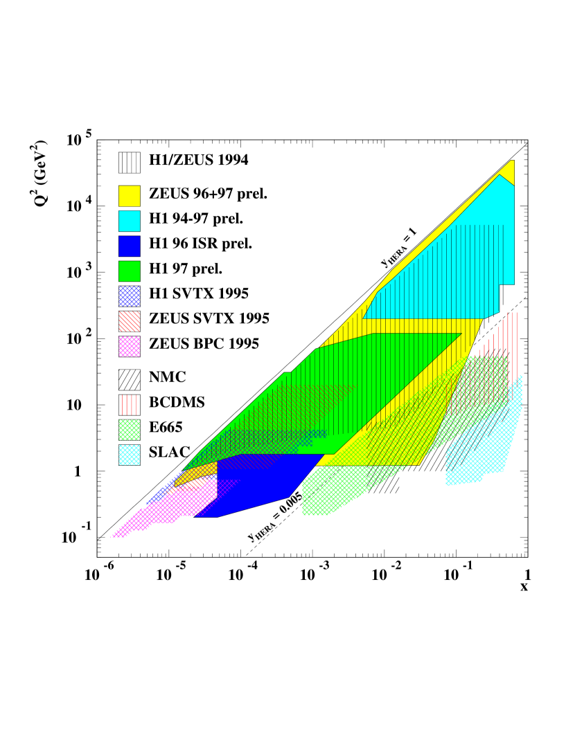
Fig. 4: The region in the $(x,Q^{2})$ plane where measurements of $F_{2}$ have been performed by the fixed target and HERA experiments.

The kinematic plane available in $x$ and $Q^{2}$ for electron-proton scattering at HERA is shown in Fig. 4.

2.2 Structure functions in the Quark Parton Model

In deep inelastic scattering (i.e. $Q^{2}\gg 1\,\mathrm{GeV^{2}}$) the nucleon is viewed as composed of point like free constituents - quarks and gluons. In the QPM the lepton nucleon interaction is described as an incoherent sum of contributions from individual free quarks. To justify this approach (?), let’s consider a virtual photon in the frame in which its four momentum is purely space-like (in the so called Breit frame). In this frame the four momenta of the photon, $q_{\gamma}$ and of the proton, $p_{p}$, have the following form:

$$q_{\gamma} = \big{(}0,0,0,-\sqrt{Q^{2}}\big{)}\,,$$

$$P_{p} = \left(\sqrt{\left(\frac{\nu^{2}}{Q^{2}}+1\right)m_{p}^{2}},0,0,\frac{m_{p}\nu}{\sqrt{Q^{2}}}\right)\,.$$ (16)

In the Bjorken limit, when $Q^{2}\sim m_{p}\nu\rightarrow\infty$ and $x=Q^{2}/(2m_{p}\nu)\sim 1$, the proton momentum $m_{p}\nu/\sqrt{Q^{2}}\rightarrow\infty$. The static photon field occupies a longitudinal size $\sim 1/\sqrt{Q^{2}}$. Because of energy conservation, the photon may only be absorbed by a quark with momentum equal to $0.5|\sqrt{Q^{2}}|$. After absorption, the quark will change direction and move with the same momentum value. The interaction time may be defined as the overlap time between the quark and the field of the photon, $t_{i}\sim 2m_{q}/Q^{2}$, where $m_{q}$ stands for some effective mass of the quark. The lifetime of the quark is then estimated to be $t_{q}\sim\sqrt{Q^{2}}/m_{q}^{2}\gg t_{i}$. Thus at large $Q^{2}$, it is indeed justified to consider the quark as free and to neglect possible interactions of the photon with other partons.

The electroweak gauge bosons couple to quarks through a mixture of vector ($v$) and axial-vector ($a$) couplings. The structure functions can then be expressed in terms of quark distributions $q_{i}(x)$, where $i$ stands for individual quark types. For non-interacting partons, as is the case in QPM, Bjorken scaling (no $Q^{2}$ dependence) is expected.

$$F_{1}(x) = \frac{1}{2}\sum_{i}q_{i}(x)(v_{i}^{2}+a_{i}^{2})\,,$$

$$F_{2}(x) = \sum_{i}xq_{i}(x)(v_{i}^{2}+a_{i}^{2})\,,$$ (17)

$$F_{3}(x) = 2\sum_{i}q_{i}(x)(v_{i}a_{i})\,.$$

The index $i$ runs over all flavors of quarks and antiquarks which are allowed, by conservation laws, to participate in the interaction. For the simplest case of electromagnetic interactions, $v_{i}=e_{i}$, where $e_{i}$ is the charge of quark $i$ in units of the electron charge, and $a_{i}=0$. For charged currents $v_{i}=a_{i}=1$ for quarks and $v_{i}=-a_{i}=1$ for antiquarks. For neutral current interactions mediated by the $Z^{0}$, $v_{i}=T_{i3}-2e_{i}\sin^{2}\Theta_{W}$ and $a_{i}=T_{i3}$, where $T_{i3}$ is the third component of the weak isospin of quark $i$ and $\Theta_{W}$ denotes the Weinberg mixing angle, one of the fundamental parameters of the Standard Model. The couplings have a more complicated structure for neutral current interactions in which the interference between the $Z^{0}$ and the $\gamma$ play an important role. A direct consequence of formulae (17), derived for spin $1/2$ partons, is the Callan-Gross relation (?), i.e.

$$2xF_{1}(x)=F_{2}(x)\,.$$ (18)

For universal parton distributions in the proton, expected in the QPM and QCD, formulae (17) can be used to relate DIS cross sections obtained with different probes. In fact, many more relations and sum rules can be derived assuming SU(3) or SU(4) flavor symmetry for hadrons. Inversely, the validity of these assumptions can be tested experimentally. A detailed discussion of these issues is beyond the scope of this review. The naive QPM approach, which allows the construction of structure functions from quark distributions, has to be altered to take into account some dynamical features predicted by QCD, such as violation of scaling and of the Callan-Gross relation, as well as higher twist effects.

Quarks are bound within the nucleon by means of gluons. We may thus expect fluctuations such as emission and reabsorption of gluons as well as creation and annihilation of $q\bar{q}$ pairs. Depending on the resolving power of the probe and the time of the interaction, some of these fluctuations can be seen and the partonic structure of the hadron will change accordingly. The structure functions acquire a $Q^{2}$ dependence. This $Q^{2}$ dependence is encoded in QCD and the measurement of the $Q^{2}$ dependence constitutes a test of perturbative QCD at a fundamental level. The violation of the Callan-Gross relation is also a consequence of QCD radiation.

Non-perturbative effects of QCD can contribute to the scale breaking of structure functions. They are due, e.g., to scattering on coherent parton states. These contributions vanish as inverse powers of $Q^{2}$. The theoretical understanding of higher twist effects is quite limited (?; ?). Experimentally they are observed at large $x$ and small $W^{2}$ (?) and are also expected to affect the very small-$x$ region (?). The assumption that quarks are massless certainly does not hold for the heavy quarks $c$, $b$ and $t$, for which $m_{c}\simeq 1.5\,\mathrm{GeV}$, $m_{b}\simeq 4.5\,\mathrm{GeV}$ and $m_{t}\simeq 175\,\mathrm{GeV}$, respectively. The radiation of heavy quarks will be affected by threshold effects which may be substantial up to large values of $Q^{2}$.

2.3 QCD evolution equations

Fig. 5: Schematic representation of photon-proton scattering for increasing photon virtuality $Q^{2}$ at fixed $W$. As $Q^{2}$ increases, the photon probes smaller transverse distance scales and is able to resolve the structure of the proton. With further increases in $Q^{2}$, quarks are resolved into more quarks and gluons.

Fig. 6: The expected behavior of the proton structure function $F_{2}$ in the QPM (top), and including the effects of QCD (adapted from figure 9.7 of ?).

The parton distributions in the hadron cannot be calculated from first principles. However, thanks to the QCD factorization theorem (?) which allows to separate the long range effects (such as the parton distribution at a small-$Q^{2}$ scale) from the short range interactions, the $Q^{2}$ dependence of partons, called parton evolution, can be calculated within perturbative QCD. The main origin of this $Q^{2}$ dependence is that a quark seen at a scale $Q^{2}_{0}$ as carrying a fraction $x_{0}$ of the proton momentum can be resolved into more quarks and gluons when the scale $Q^{2}$ is increased, as shown in Fig. 5. These quarks and gluons have $x<x_{0}$. Thus we can easily infer from this picture that the number of slow quarks will increase and the number of fast quarks will decrease when we increase the resolving power of the probe. The implications for $F_{2}$ is depicted in Fig. 6.

In QCD, as in many gauge theories with massless particles, the loop corrections to the quark gluon coupling diverge and the renormalization procedure introduces a scale into the definition of the effective coupling. The effective strong coupling constant $\alpha_{s}$ decreases with increasing scale relevant to the QCD subprocess (see Eq. (1)) and when it becomes sufficiently small, perturbative calculations can be performed.

The parton evolution equations derived on the basis of the factorization theorem are known as the Dokshitzer-Gribov-Lipatov-Altarelli-Parisi (DGLAP) evolution equations (?; ?; ?). The DGLAP equations describe the way the quark $q$ and gluon $g$ momentum distributions in a hadron evolve with the scale of the interactions $Q^{2}$.

$${\partial\over\partial\ln Q^{2}}\left(\begin{array}[]{c}q\\ g\end{array}\right)={\alpha_{s}(Q^{2})\over 2\pi}\left[\begin{array}[]{cc}P_{qq}&P_{qg}\\ P_{gq}&P_{gg}\end{array}\right]\otimes\left(\begin{array}[]{c}q\\ g\end{array}\right)\,,$$ (19)

where both $q$ and $g$ are functions of $x$ and $Q^{2}$. The splitting functions $P_{ij}$ provide the probability of finding parton $i$ in parton $j$ with a given fraction of parton $j$ momentum. This probability will depend on the number of splittings allowed in the approximation. Given a specific factorization and renormalization scheme, the splitting functions $P_{ij}$ are obtained in QCD by perturbative expansion in $\alpha_{s}$,

$$\frac{\alpha_{s}}{2\pi}P_{ij}(x,Q^{2})=\frac{\alpha_{s}}{2\pi}P_{ij}^{(1)}(x)+\left(\frac{\alpha_{s}}{2\pi}\right)^{2}P_{ij}^{(2)}(x)+\ldots\,.$$ (20)

The truncation after the first two terms in the expansion defines the next to leading order (NLO) DGLAP evolution. This approach assumes that the dominant contribution to the evolution comes from subsequent parton emissions which are strongly ordered in transverse momenta $k_{T}$, the largest corresponding to the parton interacting with the probe.

It should also be noted that beyond leading order (LO) the splitting functions depend on the factorization scale and thus the definition of parton distributions is not unique. This affects the simple relation (17) between quarks and structure functions. The relation (17) is preserved in LO, but the parton distribution functions acquire a $Q^{2}$ dependence. In NLO the Callan-Gross relation is violated. The difference between $F_{2}-2xF_{1}$ is called the longitudinal structure function $F_{L}$ (its meaning will be explained in section 2.4) and for virtual photon exchange takes the following form in QCD:

$$F_{L}=\frac{\alpha_{s}(Q^{2})}{\pi}\left[\frac{4}{3}\int_{x}^{1}\!\frac{dz}{z}\left(\frac{x}{z}\right)\!^{2}\!F_{2}(z,Q^{2})+2\!\sum_{i=1,4}e_{i}^{2}\!\int_{x}^{1}\!\frac{dz}{z}\frac{x}{z}\left(1-\frac{x}{z}\right)zg(z,Q^{2})\right]\;.$$ (21)

Formula (6) for the deep inelastic cross section remains valid to all orders.

2.4 Structure functions in the $\gamma^{*}p$ system

The lepton-nucleon interaction cross section can also be described as a convolution of a flux of virtual bosons with the absorption cross section of a virtual boson by the nucleon. This is depicted in Fig. 7 where for the sake of simplicity only $\gamma^{*}$ is considered.

Fig. 7: At small $Q^{2}$, $ep$ scattering can be thought of as 1) radiation of a virtual photon, $\gamma^{*}$, from the electron, followed by 2) $\gamma^{*}p$ scattering.

The virtual photon is treated as a massive spin 1 particle and acquires three polarization vectors corresponding to helicities $\lambda=\pm 1,~{}0$. The absorptive cross section may depend on helicity. In case of the virtual photon, parity invariance implies that the cross sections corresponding to $\lambda=\pm 1$ have to be equal. We will thus have two independent cross sections, one for absorbing a transversely polarized photon $\sigma_{T}$ ($\lambda=\pm 1$) and one for a longitudinally polarized photon $\sigma_{L}$ ($\lambda=0$). The relation between $\sigma_{T,L}$ and the structure functions $F_{1,2}$ are as follows:

$$2xF_{1} = \frac{K}{4\pi^{2}\alpha}\frac{Q^{2}}{\nu}\sigma_{T}\,,$$ (22)

$$F_{2} = \frac{K}{4\pi^{2}\alpha}\frac{Q^{2}\nu}{Q^{2}+\nu^{2}}(\sigma_{T}+\sigma_{L})\,,$$ (23)

where $K$ stands for the virtual photon flux. For virtual particles there is no unambiguous definition of the flux factor. It is a matter of convention. Here we will use the Hand convention (?) which, in analogy to the real photon case where $K=\nu$, defines $K$ for virtual photons as the energy that a real photon would need in order to create the same final state.

$$K=\nu-\frac{Q^{2}}{2m_{p}}\,.$$ (24)

The ratio $R=\sigma_{L}/\sigma_{T}$ depends on the spin of the interacting particles. A spin 1/2 massless particle cannot absorb a longitudinally polarized photon in a head-on collision without breaking helicity conservation. The early measurements in which $R$ was found to be small (?) gave support to the idea that partons in the nucleon where in fact quarks. For scalar partons $R\rightarrow\infty$. However, in a theory in which quarks are massive with mass $m_{q}$ and/or have an intrinsic transverse momentum $k_{T}$, $R$ is expected to be

$$R=\frac{\langle k_{T}^{2}\rangle+\langle m_{q}^{2}\rangle}{Q^{2}}\,.$$ (25)

The parameter $R$ can be related to the longitudinal structure function of the proton,

$$R=\frac{\left(\frac{Q^{2}}{\nu^{2}}+1\right)F_{2}-2xF_{1}}{2xF_{1}}\simeq\frac{F_{L}}{2xF_{1}}\,.$$ (26)

As an outcome of QCD radiation partons in the proton acquire transverse momentum, the more so the slower they are, and therefore $F_{L}$ is non-zero.

The representation of structure functions in terms of absorption cross sections turns out to be very useful in understanding some dynamical properties of DIS as it creates a natural link between the perturbative regime of QCD and the non-perturbative soft hadron-hadron interactions. The latter are best described in the framework of Regge theory.

2.5 Regge phenomenology

The soft hadron-hadron interactions are well described by Regge phenomenology (?) in which the interaction is viewed as due to exchanges of collective states called Regge poles. The Regge poles can be classified into different families according to their quantum numbers. The Regge poles with quantum numbers of mesons form linear trajectories in the $m^{2},l$ plane, where $m$ is the mass of the meson and $l$ its spin. The continuation of a trajectory to negative values of $m^{2}$ leads to a parameterization in terms of $t$, the square of the four momentum transfer, as follows:

$$\alpha(t)=\alpha_{0}+\alpha^{\prime}\cdot t\,,$$ (27)

where $\alpha_{0}$ is the intercept and $\alpha^{\prime}$ is the slope of the trajectory.

Fig. 8: Example of the $\rho$ (circles), $\omega$ (empty squares), $\phi$ (triangles) and $\pi$ (dots) trajectories. Also shown is the continuation of the $\rho$ trajectory as measured in $\pi^{-}p\rightarrow\eta n$ (?).

An example of such trajectories, called reggeon trajectories, is shown in Fig. 8. Among all possible families of Regge poles there is a special one, with the quantum numbers of the vacuum, called the pomeron ($I\!\!P$) trajectory. There are no known hadronic bound states lying on this trajectory (glue-balls would be expected to form this trajectory). Its parameters have been determined experimentally (?; ?; ?) to be

$$\alpha_{I\!\!P}=1.08+0.25t\,.$$ (28)

In Regge theory the energy dependence of total and elastic cross sections is derived from the analytic structure of the hadronic amplitudes. In the limit $s\gg-t$, where $s$ is the square of the center-of-mass energy of the scattering, the amplitude for elastic scattering has the form $A(s,t)\propto s^{\alpha_{I\!\!P}(t)}$. The pomeron trajectory also provides the leading contribution to the high energy behavior of the total cross section,

$$\sigma_{\mathrm{tot}}=s^{-1}{\it Im}A(s,t=0)\propto s^{\alpha_{{\scriptscriptstyle I\!\!P}}(0)-1}$$ (29)

The $s$ dependence of hadronic interactions fulfills this behavior independently of the interacting particles (?) as expected from the universality of the exchanged trajectories.

Two types of soft interactions arise naturally in Regge theory: elastic and diffractive scattering. These are mediated by the exchange of the pomeron. In elastic scattering, the square of the momentum transfer, $t$, between the interacting hadrons is very small and the only products of this interaction are the two hadrons which emerge with little change in their initial directions. The properties of the elastic scattering cross section determine the slope of the pomeron trajectory. In diffractive scattering, the momentum transfer between initial hadrons still remains very limited, but one or both of the interacting hadrons may be excited into a state of finite mass which then subsequently decays. Single dissociation occurs if only one hadron dissociates, while if both dissociate into higher masses the scattering is called double dissociation. Typical of diffractive scattering is the production of relatively low excited masses and the mass spectrum is directly related to the properties of the pomeron trajectory.

Regge phenomenology proved very successful in describing the energy dependence of the total hadron-hadron interaction cross section as well as in describing the properties of elastic and diffractive scattering (for a review see ?).

2.6 QCD dynamics at small $x$

In deep inelastic scattering, the kinematic region which corresponds to the Regge limit is that of small $x$ at fixed $Q^{2}$. In perturbative QCD at small $x$, higher-loop contributions to the splitting functions are enhanced,

$$P_{ij}^{(n)}\sim\frac{1}{x}\ln^{(n-1)}x\,.$$ (30)

The presence of these terms may spoil the convergence of (20). The evolution equation which allows the resummation in the expansion (20) of leading $(\alpha_{s}\ln x)^{n}$ terms is known under the name of Balitsky-Fadin-Kuraev-Lipatov (BFKL) equation (?; ?; ?). In the parton cascade picture this evolution corresponds roughly to cascades with subsequent emissions following a strong ordering in $x$ with no restriction on the $k_{T}$. Here the evolution takes place from high longitudinal momentum partons to low longitudinal momenta over a fixed transverse area proportional to $1/Q^{2}$. The BFKL equation in its original form does not address the $Q^{2}$ evolution of the parton distributions. The difference between DGLAP and BFKL evolution is shown schematically in Fig. 9.

Fig. 9: Schematic description of the differences in the DGLAP and BFKL evolution equations. The DGLAP equation has strong $Q^{2}$ ordering in the radiation sequence, while BFKL evolution has strong $x$ ordering.

The two approaches to parton evolution, DGLAP and BFKL, are embedded in a single equation known as the CCFM equation (?; ?; ?) based on $k_{T}$ factorization and angular ordering.

The solutions of the DGLAP equations and of the BFKL equation (in LO), in the limit of very small $x$, where the dominant contribution to the cross section is driven by gluon radiation, predict a rise of $F_{2}$ with decreasing $x$,

$$F_{2}^{DLL}(x,Q^{2})\sim\exp\left(2\sqrt{\frac{C_{A}\alpha_{s}}{\pi}\ln\frac{1}{x}\ln\frac{Q^{2}}{Q^{2}_{0}}}\right)\,,$$ (31)

$$F_{2}^{BFKL}(x,Q^{2})\sim\sqrt{\frac{Q^{2}}{Q^{2}_{0}}}x^{-\frac{4C_{A}\alpha_{s}}{\pi}\ln 2}\,,$$ (32)

where the superscript $DLL$ stands for the double leading logarithmic approximation used in solving the DGLAP equation and $Q_{0}^{2}$ denotes the starting scale of the evolution. In general the BFKL equation predicts a faster increase of $F_{2}$ with decreasing $x$ and stronger scaling violations in $Q^{2}$ as compared to the DGLAP evolution. However the solution (32) is derived assuming a constant $\alpha_{s}$ and higher order corrections are expected to tame the rise with $1/x$ (for a discussion see ?). In the BFKL approach the concept of a QCD pomeron arises naturally.

The two solutions presented above (31, 32) are expected to violate unitarity at very small $x$ (?). The fast increase of parton densities at small $x$ expected in perturbative QCD and confirmed experimentally (see section 4) raise a natural question, whether such high densities will not lead to overcrowding of the proton. The annihilation and recombination of partons could lead to saturation effects and would require corrections to the known evolution equations (?).

2.7 Perturbative QCD in the final states

It is generally believed that the pattern of perturbative QCD radiation should be observed in the hadronic final states. Although colored partons cannot be observed directly, their fragmentation produces jets of hadrons, collimated around the original direction of the partons. This is the principle of parton-hadron duality (?). In fact, while the need for gluons was inferred from DIS measurements of structure functions, the actual proof of their existence was first made in the $e^{+}e^{-}$ interactions (for a review see ?). Hadron production in high energy $e^{+}e^{-}$ interactions proceeds through the annihilation of leptons into a photon (or a $Z^{0}$) with a subsequent production of a $q\bar{q}$ pair. The fragmentation of the pair leads to a two jet structure in the final state. However, each of the quarks (or both) may emit a gluon with a large transverse momentum relative to the parent quark. Such a hard gluon will be a source of a third jet. The probability of such a configuration can be calculated in perturbative QCD.

A similar situation may arise in DIS. In a typical DIS interaction we expect the final state to consist of a jet of hadrons originating from the struck quark, called the current jet, which balances in transverse momentum the scattered lepton. The remnant of the target also fragments into hadrons which remain collimated around the direction of the latter. The space between the fragmentation of the current jet and the remnant is filled by radiation due to the color flow between the struck quark and the remnant state of the target. Various approaches exist to model this effect (?; ?).

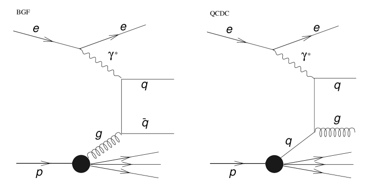
Fig. 10: Diagrams for boson-gluon fusion (BGF) and for QCD Compton (QCDC) processes in DIS.

A gluon may split into a pair of quarks with large relative transverse momenta, before one of the quarks absorbs the virtual boson. Two jets will be observed in the final state. This process, called boson-gluon fusion (BGF),is diagrammatically presented in Fig. 10. Another possibility is that the quark will emit a hard gluon before absorbing the virtual boson as shown in Fig.  10b. This process is called QCD Compton scattering (QCDC). The contribution of both diagrams to the DIS cross section can be calculated in perturbative QCD (?).

In BGF the large transverse momenta partons may be replaced by heavy quark production. The latter in particular gives rise to the charm content of the $F_{2}$ structure function. Both the QCDC and BGF processes are included at some level in the evolution equation in the NLO approximation (?). The BGF process is sensitive to the gluon content of the nucleon. The extraction of the gluon distribution from a direct measurement of the BGF process is quite challenging because of higher order QCD corrections, especially when the square of transverse momenta of the jets is of the same order as $Q^{2}$. However heavy quark production through the BGF mechanism is easier to control theoretically (?; ?).

The perturbative calculation of cross sections for QCDC or BGF type of processes does not require $Q^{2}$ to be large. In fact the presence of one large scale, be it transverse momentum or heavy quark mass, is sufficient to perform perturbative calculations, even for the case of $Q^{2}\simeq 0\,\mathrm{GeV^{2}}$.

As has been mentioned earlier charged leptons are a natural source of a flux of photons and the propagator effect favors photons with $Q^{2}\simeq 0\,\mathrm{GeV^{2}}$. At HERA, electroproduction events with $Q^{2}\sim 0\,\mathrm{GeV^{2}}$ are called photoproduction events. In QCD the production of large transverse momentum jets in photoproduction is very similar to jet production in hadron-hadron interactions, which are sensitive to the parton distributions in the hadrons. Thus, in lepton-hadron interactions, the study of the structure of matter can be extended to include the structure of the photon.

2.8 Space time picture of $ep$ scattering at HERA

In discussing the QPM picture of DIS we have presented arguments why a virtual photon was able to resolve substructures inside the nucleon and why the interaction could be viewed as an incoherent sum of elastic $eq\rightarrow eq$ scattering. For the latter we argued in the Breit frame where it is easy to depict DIS scattering. We could go one step further and ask what would the hadronic final state look like in such an approach. In the Breit frame the quark which absorbed the virtual boson moves in the opposite direction to the remnant of the target nucleon. The two states are each colored and we expect radiation, which eventually turns into hadrons, to fill up the rapidity space between them. Thus in the HERA frame of $ep$ interactions we expect the hadronic final state to consist of a jet of hadrons originating from the fragmentation of the scattered quark which balances the transverse momentum of the electron, a jet of particles around the original direction of the proton and some hadronic activity between the two. This is schematically depicted in Fig. 11.

Fig. 11: Schematic representation of the expected energy flow in deep inelastic scattering. The need for color flow between the struck quark and proton remnant generates particles distributed in rapidity (or pseudorapidity, $\eta$) between these.

It is also of interest to consider $ep$ scattering in the rest frame of the target. We will be mainly interested in the fate of the photon in this frame and the coordinate system will be rotated such that the virtual photon moves along the $z$ axis. The four momentum vector of the photon in this frame is

$$q=(\nu,0,0,\sqrt{\nu^{2}+Q^{2}})\,.$$ (33)

According to quantum mechanics, we can think of the photon as fluctuating with some probability into states of $q\bar{q}$, $e^{+}e^{-}$, $\mu^{+}\mu^{-}$, etc… The life time of such a quantum mechanical fluctuation is given by the Heisenberg uncertainty principle,

$$\tau\simeq\frac{1}{E_{f}-\nu}\,,$$ (34)

where $E_{f}$ is the energy of the state of mass $M_{f}$ in which the photon happened to fluctuate. Here we will concentrate on the hadronic fluctuation of the photon. For large $\nu$ the expression can be approximated by

$$\tau\simeq\frac{2\nu}{M_{f}^{2}+Q^{2}}\,,$$ (35)

where $M_{f}$ depends on the initial configuration of the $q\bar{q}$ system (for a derivation see for example ?),

$$M_{f}^{2}=\frac{m_{q}^{2}+k_{T}^{2}}{z(1-z)}\,,$$ (36)

where $m_{q}$ is the mass of the quarks, $k_{T}$ their transverse momentum relative to the photon and $z$ is the fraction of the photon momentum carried by one of the quarks.

The first observation we can make based on expression (35) is that the life time of a hadronic fluctuation of the photon increases as its energy increases and decreases as $Q^{2}$ increases. If the hadronic fluctuation lives long enough to overlap with the size of the target the interaction of the photon will proceed through its hadronic component. In the early days it was natural to assume that the photon would turn into a vector meson, preferably the $\rho^{0}$ meson as the one with the lowest mass. This was the essence of the Vector Dominance Model (VDM) (?) which explained why real photons behaved as hadrons. The fact that with increasing $Q^{2}$ the life time of a hadronic fluctuation would decrease made it natural to view the virtual photon as a point like probe. However, it was also realized (?) that at sufficiently large $\nu$ a virtual photon could acquire hadronic properties.

When QCD is turned on, the whole picture acquires even more substance. As a consequence of the renormalizability of QCD, fluctuations with $M_{f}^{2}\gg Q^{2}$ can be neglected and $M_{f}^{2}$ may be approximated by $Q^{2}$ (?; ?), in which case expression (35) can be reduced to the form

$$\tau\simeq\frac{1}{2m_{p}x}\,.$$ (37)

To quantify this relation, at $x=0.1$ the longitudinal dimension of the hadronic fluctuation is of the order of 1 fm, the typical size of a hadronic target. Thus it becomes clear that at small $x$, independently of $Q^{2}$, the hadronic fluctuations of the photon have to be resurrected with important consequences for the physics of small-$x$ DIS interactions.

Until now, we have tacitly assumed that any fluctuation into a $q\bar{q}$ pair will lead the photon to look like a hadron. This turns out not to be the case in QCD. For the sake of simplicity we consider two extreme cases of the $q\bar{q}$ initial configuration, one where the initial $k_{T}$ is small and one where it is large. If the $k_{T}$ is small the $q\bar{q}$ form a large size object (for fixed $M_{f}$, small $k_{T}$ implies very different $z$ and $(1-z)$ values such that the $q$ and $\bar{q}$ are moving at very different speeds.) The color dipole moment is large and given enough time the space will be filled by gluon radiation. This fluctuation is likely to acquire hadron like properties and interact with the target as in hadron-hadron interactions. The slower quark is expected to interact with the target while the faster one continues in the original direction of the photon and fragments into hadrons.

If $k_{T}$ is large, then $z$ and $(1-z)$ have similar values and the $q$ and the $\bar{q}$ are spatially close to each other. The effective charge of such a dipole is very small and thus their interaction cross section is expected to be small. Such a small size wave packet can resolve the partonic structure of the target hadron. This is the essence of what is called the color transparency phenomenon. It has been shown that the interaction cross section of a small size colorless configuration is proportional to the gluon distribution in the target (?),

$$\sigma_{T}^{q\bar{q}}=\frac{\pi^{2}}{3}\alpha_{s}b^{2}xG_{T}(x,9/b^{2}),$$ (38)

where $b$ is the transverse separation between the $q\bar{q}$ system and $G_{T}$ stands for the gluon distribution in the target. Thus effectively the contribution of small size configurations to the cross section may be large when the density of gluons is large.

In summary, for $Q^{2}\sim 0\,\mathrm{GeV^{2}}$ the photon acquires a hadronic structure. We thus expect features very similar to the ones observed in hadron-hadron interactions, including hard scattering between the parton content of the hadronic fluctuation of the photon and the hadron target. These hard processes are called resolved photon processes. An additional component is due to interactions of a photon which fluctuated into a small size configuration, which gives rise to the anomalous component of the photon structure.

The picture emerging in DIS is very similar to that derived from the QPM in the Breit frame. Because of the dominance of small $k_{T}$ configurations to the cross section, corresponding to asymmetric parton configurations in the photon fluctuation, the final state consists of a current jet and proton remnant. However, the hadronic nature of the interaction implies that we should expect the same type of contributions as in hadron-hadron interactions. In particular, the presence of diffractive states, with large rapidity gaps separating the photon and the proton fragmentation regions are very natural, while they are hard to predict in the QCD improved parton model, where the presence of large rapidity gaps is strongly suppressed.

QCD corrections to the simple QPM picture arise naturally when small size $q\bar{q}$ configurations are allowed. In fact they give rise to a special new class of perturbative interactions such as diffractive production of jets or the exclusive production of vector mesons by longitudinally polarized photons, mediated by two-gluon exchange.

In this approach, it also becomes clear that DIS scattering, in particular at small $x$, is a result of an interplay of soft and hard interactions.

3 Experimental aspects

3.1 The HERA accelerator

The HERA (Hadron-Electron Ring Anlage) machine is the world’s first lepton-nucleon collider (?; ?; ?; ?). It is located in Hamburg, Germany, and has been providing luminosity to the colliding beam experiments H1 and ZEUS since the summer of 1992. It is schematically shown in Fig. 12, along with the pre-HERA accelerator elements. The basic HERA operational parameters are given in Table 1. HERA was approved in 1984, and was built on schedule. The electron machine was first commissioned in 1989, while the proton ring was first operated in March 1991. First electron-proton collisions were achieved in October 1991. Following this commissioning of HERA, the two colliding beam detectors ZEUS and H1 moved into position to record data.

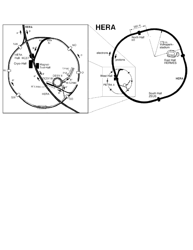
Fig. 12: The layout of HERA is shown on the right, along with the location of the different detector halls. The pre-accelerators are shown in the blowup on the left.

Table 1: The main HERA parameters as of the end of the 1997 running period.

Parameter	Achieved
$E_{p}$ (GeV)	$820$
$E_{e}$ (GeV)	$27.5$
$I_{e}$ (mA)	$40$
$I_{p}$ (mA)	$100$
# bunches	$189$
Time between crossings	$96$ ns
$\sigma_{x}$ at IP ($\mathrm{\mu m}$)	$179$
$\sigma_{y}$ at IP ($\mathrm{\mu m}$)	$48$
$\sigma_{z}^{\mathrm{proton}}$ at IP (mm)	$200$
${\mathcal{L}}_{\mathrm{inst}}$ ($\mathrm{cm^{-2}\,s^{-1}})$	$1.4\cdot 10^{31}$

The HERA electron ring operates at ambient temperatures, while the proton ring is super-conducting. The two beam pipes merge into one at two areas along the circumference. The beams are made to collide at zero crossing angle to provide $ep$ interactions for the experiments H1 and ZEUS. These detectors will be described in more detail in further sections. The electrons (positrons) and protons are bunched, with bunches within one bunch train separated by $96$ ns. Some number of bunches are left unpaired (i.e., the corresponding bunch in the other beam is empty) for background studies. The electron (positron) beam is polarized up to $70$ % in the transverse direction via the Sokholov-Ternov effect (?). A third experiment, HERMES (?), makes use of this polarized beam by colliding it with a polarized proton gas jet to study the spin structure of the proton. A fourth experiment, HERA-B (?), is currently being assembled. It uses wire targets in the proton beam to study B hadron production and decay with large statistics in an effort to find CP violation in the B hadron sector.

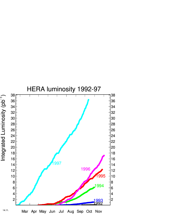
Fig. 13: The integrated luminosity delivered by HERA versus the date for the years since the start of HERA operation.

The integrated luminosities per year are shown in Fig. 13 as a function of the day of the run. These luminosity profiles are comparable to those achieved at other successful accelerator facilities such as LEP (CERN, Geneva) or the Tevatron (FNAL, USA). Note that HERA initially began as an electron-proton collider, but switched to positron-proton collisions in 1994 once it was determined that the electron lifetime was severely limited at high currents. It is thought that this is the result of electrons interacting with positively charged “macro”-particles in the beam pipe. New pumps have been installed in the electron ring in the 1997/1998 shutdown to cure this problem. In its 1997 configuration, HERA accelerated protons to $820$ GeV and positrons to $27.5$ GeV. The proton beam energy has been increased to $920$ GeV as of August 1998. The maximum instantaneous luminosity achieved so far is ${\mathcal{L}}=1.4\cdot 10^{31}$ cm^-2 s^-1 with 174 colliding bunches of electrons and protons, to be compared with a design goal of ${\mathcal{L}}=1.5\cdot 10^{31}$ cm^-2 s^-1 with 210 colliding bunches. There is a significant luminosity upgrade program planned for the HERA accelerator which should result in luminosities of ${\mathcal{L}}=7.5\cdot 10^{31}$ cm^-2 s^-1. This upgrade is currently planned for the 1999/2000 break. Another planned upgrade is the introduction of spin rotators to provide longitudinal polarization to the colliding beam experiments. These upgrades are described in more detail in section 9.

3.2 The detectors H1 and ZEUS

In this section, we briefly review the properties of the two colliding beam detectors H1 and ZEUS, run by the eponymous collaborations. Both are general purpose magnetic detectors with nearly hermetic calorimetric coverage. They are differentiated principally by the choices made for the calorimetry. The H1 collaboration has stressed electron identification and energy resolution, while the ZEUS collaboration has put its emphasis on optimizing the calorimetry for hadronic measurements. The detector designs reflect these different emphases. The H1 detector has a large diameter magnet encompassing the main liquid argon calorimeter, while the ZEUS detector has chosen a uranium-scintillator sampling calorimeter with equal response to electrons and hadrons. The detectors are undergoing continuous changes, with upgrades being implemented and some detector components being removed or simply not used.

We review here the capabilities of the two different detectors for tracking of charged particles, energy measurements, and particle identification. For detailed information on the detectors, the reader should refer to the technical proposals and status reports: H1 (?; ?) and ZEUS (?; ?).

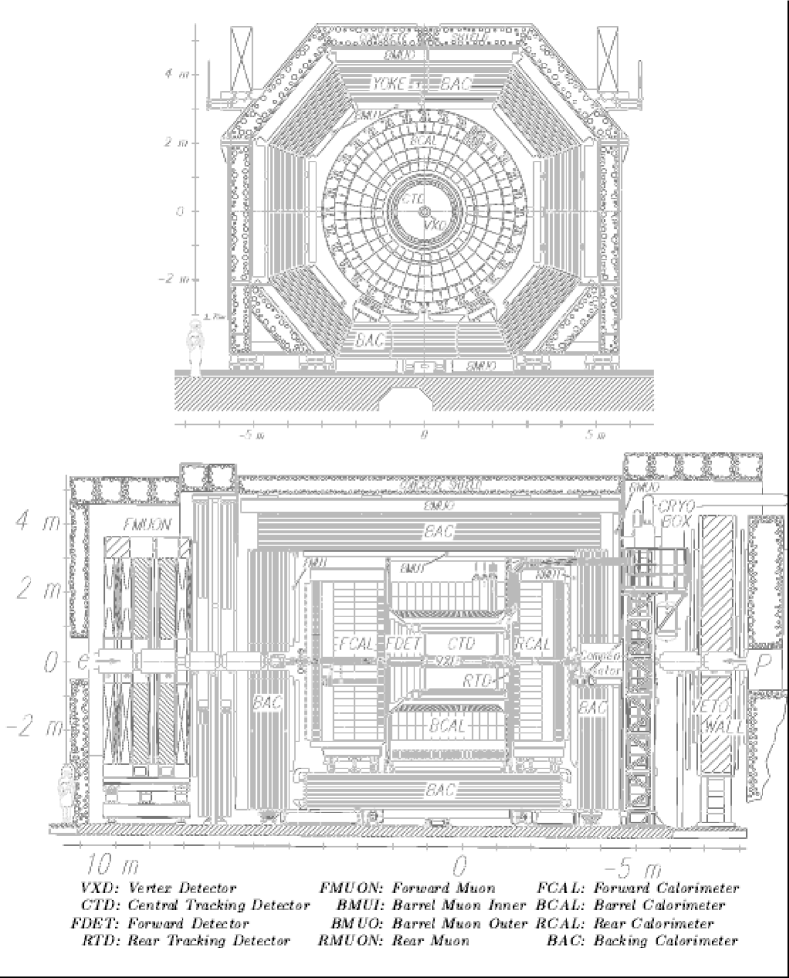
Fig. 14: Cross sectional views of the ZEUS detector.

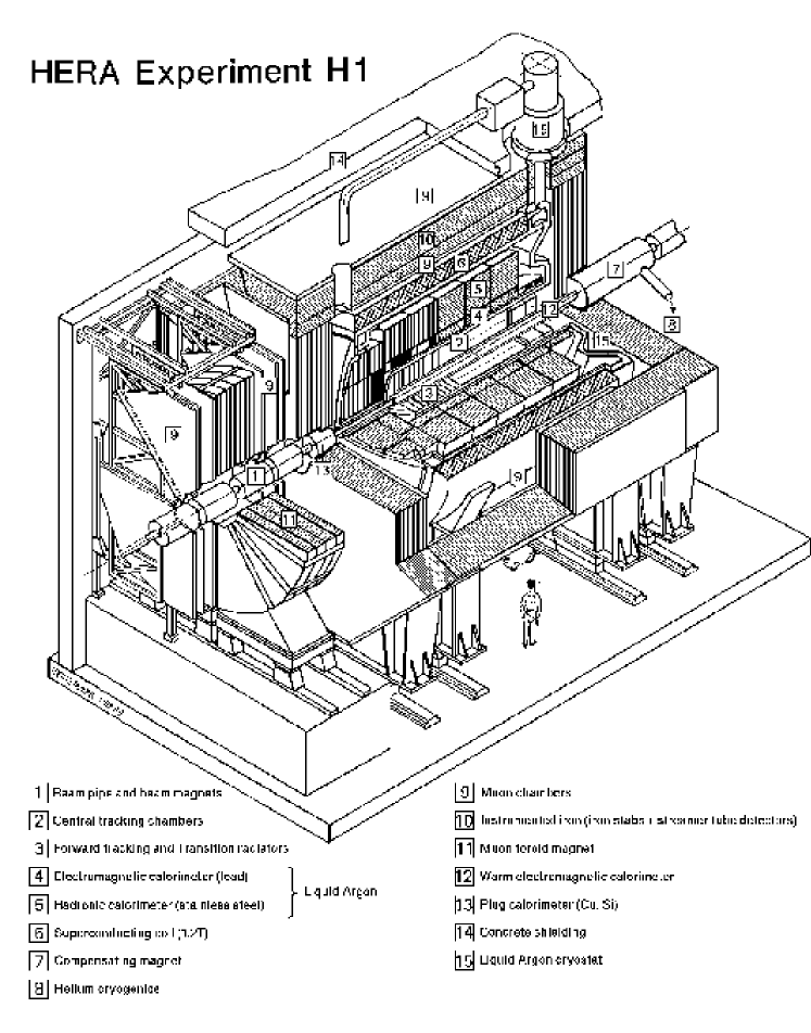
Fig. 15: Schematic drawing of the H1 detector.

Table 2: The principal H1 central detector parameters (1997 status).

Component	Parameter	Value	Comment
LAr	Angular coverage	$4^{\circ}\leq\theta\leq 154^{\circ}$	ref (?)
Calorimeter	$\sigma/E$(EM showers)	$0.12/\sqrt{E(\mathrm{GeV})}\oplus 0.01$	test beam (?)
			(?)
	EM E scale uncertainty	$1-3$ %	ref (?)
	$\sigma/E$(Hadronic showers)	$0.50/\sqrt{E(\mathrm{GeV})}\oplus 0.02$	test beam (?)
			(?)
	had E scale uncertainty	$4$ %	ref (?)
	angular resolution	$2\,\mathrm{mrad}$	$\theta<30^{\circ}$
	angular resolution	$<5\,\mathrm{mrad}$	$\theta>30^{\circ}$
SPACAL	Angular coverage	$153^{\circ}\leq\theta\leq 177.8^{\circ}$	ref (?)
	$\sigma/E$(EM showers)	$0.075/\sqrt{E(\mathrm{GeV})}\oplus 0.025$	in situ (?)
	EM E scale uncertainty	$1\rightarrow 3$ %	ref (?)
	had E scale uncertainty	$7$ %	ref (?)
	spatial resolution	$4\,\mathrm{mm}$	ref (?)
	time resolution	$<1$ ns	ref (?)
Central	B-field (Tesla)	$1.15$
Tracking	angular coverage	$15^{\circ}<\theta<165^{\circ}$
	$\sigma/p_{T}$	$0.01\cdot p_{T}(\mathrm{GeV})$	Full length tracks (?)
Luminosity	normalization uncertainty	$1.5$ %	ref  (?)

Table 3: The principal ZEUS central detector parameters (1997 status).

Component	Parameter	Value	Comment
Calorimeter	Angular coverage	$2.6<\theta<176.2^{\circ}$	Extended to $178.4^{\circ}$ in 1995
	$\sigma/E$(EM showers)	$0.18/\sqrt{E(\mathrm{GeV})}\oplus 0.02$	test beam (?)
			(?)
	EM E scale uncertainty	$1-3$ %	ref (?)
	$\sigma/E$(Hadronic showers)	$0.35/\sqrt{E(\mathrm{GeV})}\oplus 0.03$	test beam (?)
			(?)
	had E scale uncertainty	$3$ %	ref (?)
	position resolution	$\sim 1\,\mathrm{cm}$	EM showers, ref (?)
	time resolution	$<1\,\mathrm{ns}$	for $E>4.5\,\mathrm{GeV}$
Central	B-field (Tesla)	$1.43$
Tracking	angular coverage	$11^{\circ}<\theta<168^{\circ}$
	$\sigma/p_{T}$	$0.005\cdot p_{T}(\mathrm{GeV})\oplus 0.016$	Full length tracks (?)
	$z$ vertex resolution	$0.4\,\mathrm{cm}$	Full length tracks, $p_{T}>5\,\mathrm{GeV}$
	$R-\phi$ vertex resolution	$0.1\,\mathrm{cm}$	Full length tracks, $p_{T}>5\,\mathrm{GeV}$
Luminosity	normalization uncertainty	$1.5$ %	ref  (?)

A cross sectional view of the ZEUS detector is presented in Fig. 14. The H1 detector is shown in Fig. 15. The ZEUS detector consists of tracking chambers inside a superconducting solenoidal magnet, surrounded by calorimeters and muon chambers. The H1 detector has several different tracking detectors inside the calorimeter. The superconducting solenoid is placed outside the calorimeter to minimize the amount of inactive material in the path of electrons. Not shown in the figures are luminosity detectors and electron detectors downstream in the direction of the electron beam, and a proton spectrometer and neutron calorimeter in the direction of the proton beam. The principal central detector parameters are given in Tables 2 and  3.

3.2.1 The tracking detectors

The ZEUS tracking detectors consist of a vertex detector (VXD), a central tracking detector (CTD), and forward and rear tracking detectors (FTD,RTD).

The VXD is a jet chamber with small layer spacing ($3$ mm), which allows the measurement of 12 coordinates within the range $10.0<R<15.6$ cm, and the slow drift gas (dimethyl ether) gives a resolution $30$ $\mu$m at the center of the cell. The VXD, in conjunction with the CTD, has an impact parameter resolution of $40$ $\mu$m for high momentum tracks. The VXD was in operation since the beginning of data taking, but has been removed at the end of the 1995 running period.

The CTD is a drift chamber composed of 9 “super” layers, each consisting of 8 wire layers. Of these, 5 are axial (along the $z$-axis ) superlayers and 4 stereo, allowing both an $R-\phi$ and a $z$ coordinate measurement. The CTD has cells oriented at a $45^{\circ}$ angle to the radial direction to produce drift lines approximately tangential to the chamber azimuth in the strong axial magnetic field ($1.43$ T) provided by the superconducting solenoid. This cell orientation also guarantees that at least one layer per superlayer will have a drift time shorter than the bunch crossing interval of 96 ns. The CTD has a design momentum resolution in a $1.7$ Tesla magnetic field of

$$\sigma/p=0.002p(\mathrm{GeV})\oplus 0.003$$ (39)

at $\theta=90^{\circ}$, and a z coordinate resolution of $1$ mm from the stereo wires. In addition to its primary function of measuring the momentum of charged particles, the CTD also provides particle identification information via $dE/dx$. A resolution of

$$\frac{\sigma(dE/dx)}{(dE/dx)}=0.06$$ (40)

is expected.

The FTD consists of 3 planar drift chambers and extends the tracking region in the forward region to $7.5^{\circ}<\theta<28^{\circ}$, where high particle densities are expected due to the Lorentz boost in the proton beam direction. The transition radiation detector (TRD), a tool for identifying electrons in the forward direction, is placed between the FTD chambers. The RTD consists of one plane of drift chambers covering the angular range $160^{\circ}<\theta<170^{\circ}$. Each of the FTD and RTD drift chambers consists internally of three layers of drift cells, with the second and third wire layers rotated by $+60^{\circ},-60^{\circ}$ with respect to the first layer. The design resolution is $120-130$ $\mu$m, and the two-track resolution is $2.4$ mm.

The H1 tracking detectors consist of central jet chambers (CJC1,CJC2), central trackers for measuring the z coordinate (CIZ,COZ), forward tracking detectors (FTD), rear tracking detectors (BDC), and central and rear silicon microvertex detectors (CST, BST).

The central jet chambers (CJC1,CJC2) are two large, concentric drift chambers. The inner chamber, CJC1, has 24 layers of sense wires arranged in 30 phi cells, while CJC2 has 32 layers of sense wires in 60 phi cells. The cells are at a 30^∘ angle to the radial direction. The point resolution is $170\;\mu$m in the $R-\phi$ direction. The $z$ coordinate is measured by charge division and has an accuracy of $22$ mm. Test beam results indicate a momentum resolution for the CJC of

$$\sigma/p=0.003p(\mathrm{GeV})\,.$$ (41)

The $dE/dx$ resolution is expected to be $6$ %, as for the ZEUS CTD.

The CIZ and COZ are thin drift chambers with sense wires perpendicular to the beam axis, and therefore complement the accurate $R-\phi$ measurement provided by the CJC by providing accurate $z$ coordinates. The CIZ is located inside the CJC1, while COZ is located between CJC1 and CJC2. These two chambers deliver track elements with typically $300$ $\mu$m resolution in $z$.

The forward tracking detectors (FTD) are integrated assemblies of three supermodules, each including, in order of increasing $z$: three different orientations of planar wire drift chambers (each rotated by $60^{\circ}$ to each other in azimuth), a multiwire proportional chamber (FWPC) for fast triggering, a transition radiation detector and a radial wire drift chamber. The FTD is designed to give a momentum resolution of

$$\sigma/p=0.003p(\mathrm{GeV})$$ (42)

and track angular separation $\sigma_{\theta,\phi}<1$ mrad.

A backward proportional chamber (BPC) located just in front on the rear calorimeter provided an angular measurement of the electron, together with the vertex given by the main tracking detectors. This detector has been replaced in the 1994/95 shutdown by an eight layer drift chamber (BDC) with a polar angle acceptance between $155.1<\theta<177.5^{\circ}$  (?).

3.2.2 Calorimetry

The ZEUS tracking detectors are surrounded by a ²³⁸U-scintillator sampling calorimeter, covering the angular range $2.2^{\circ}<\theta<176.5^{\circ}$. This calorimeter design was chosen to give the best possible energy resolution for hadrons. The calorimeter consists of a forward part (FCAL), a barrel part (BCAL), and a rear part (RCAL), with maximum depths of $7.1\lambda,\;5.3\lambda,\;{\rm and}\;4.0\lambda$, respectively. The FCAL and BCAL are segmented longitudinally into an electromagnetic section (EMC), and two hadronic sections (HAC1,2). The RCAL has one EMC and one HAC1 section. The cell structure is formed by scintillator tiles; cell sizes range from $5\times 20$ cm² (FEMC) to $24.4\times 35.2$ cm² at the front face of a BCAL HAC2 cell. The light generated in the scintillator is collected on both sides of the module by wavelength shifter (WLS) bars, allowing a coordinate measurement based on knowledge of the attenuation length in the scintillator. The light is converted into an electronic signal by photomultiplier tubes (PMTs).

The performance of the calorimeter has been measured in detail in test beams, and some results are summarized in Table 3. The signal from the ²³⁸U radioactivity has proven to be an extremely valuable calibration and monitoring tool. The uranium activity signal is reproducible to better than $0.2$ %. Test beam studies have shown that the inter calibration between cells of a module, and from module to module, is known at the $1$ % level by setting the PMT gains in such a way as to equalize the uranium signal. Despite the presence of the uranium activity, the calorimeter has very low noise (typically $10$ MeV for an EMC PMT and $20$ MeV for a HAC PMT).

The angular coverage in the electron beam direction was extended in the 1994/1995 shutdown with the addition of a small Tungsten-scintillator calorimeter (BPC) located behind the RCAL at $z=294$ cm, and within $4.4$ cm of the beam. This calorimeter (?) measures electrons in the angular range $15$ to $34$ mrad.

Particle identification in the uranium calorimeter is enhanced by the addition of a silicon pad array (HES) near shower maximum in the RCAL and FCAL. All RCAL modules have been instrumented with these $3\times 3.3$ cm² pads, while the FCAL is to be completed in the 1997/1998 shutdown. This detector is expected to improve electron recognition in jets by a factor of 10 to 20.

The high resolution calorimeter is surrounded by the backing calorimeter (BAC). The BAC is formed by instrumenting the yoke used to guide the solenoidal field return flux, and consists of $40,000$ proportional tubes and $1,700$ pad towers, allowing an energy resolution of $\sigma/E=1.1/\sqrt{E}$. The backing calorimeter allows for the correction or rejection of showers leaking from the uranium calorimeter. It is also useful for identifying muons.

The H1 detector places emphasis on electron recognition and energy measurement. This led to placing the calorimeter inside the coil providing the axial field for the tracking detectors. Liquid argon (LAr) was chosen because of its good stability, ease of calibration, fine granularity and homogeneity of response. The LAr calorimeter covers the polar angle range between $4^{\circ}<\theta<154^{\circ}$. The segmentation along the beam axis into “wheels” is eightfold, with each wheel segmented into octants in $\phi$. The hadronic stacks are made of stainless steel absorber plates with independent readout cells inserted between the plates. The orientation of the plates varies with $z$ such that particles always impact with angles greater than $45^{\circ}$. The structure of the electromagnetic stack consists of a pile of G10-Pb-G10 sandwiches separated by spacers defining the LAr gaps. The granularity ranges from $10\rightarrow 100$ cm² in the EMC section, to $50\rightarrow 2000$ cm² in the HAC section. Longitudinal segmentation is 3–4 fold in the EMC over 20–30 radiation lengths and 4–6 fold in the HAC over 5–8 interaction lengths. The LAr calorimeter has a total of $45,000$ readout cells. The noise per cell ranges from $15\rightarrow 30$ MeV. The resolution measured in the test beam is given in Table 2. The calorimeter is non-compensating, with the response to hadrons about $30$ % lower than the response to electrons of the same energy. An offline weighting technique is used to equalize the response and provide the optimal energy resolution.

The polar angle region $151^{\circ}<\theta<176^{\circ}$ of the H1 detector contains the backward electromagnetic calorimeter (BEMC). This is a conventional lead-scintillator sandwich calorimeter used to measure the scattered electron for $Q^{2}\leq 100$ GeV². The calorimeter has a depth of $21.7\;X_{0}$, or approximately $1$ hadronic interaction length, which on average contains 45 % of the energy for a hadronic shower. The detector is composed of $8\times 8$ cm² stacks read out by wavelength shifter and photodiodes. It has a two-fold segmentation in depth. The energy resolution is found to be

$$\sigma/E=10~{}\%/\sqrt{E({\rm GeV})}\oplus 1.7~{}\%\;\;\;.$$ (43)

The position resolution is $7$ mm for high energy electrons. The average noise per stack was measured to be $130$ MeV. The stack-to-stack calibration was performed using so-called kinematic peak events, for which the electron has a well-defined energy, and is better than $1$ %.

The BEMC was replaced in the 1994/1995 shutdown with a lead/scintillating fiber calorimeter (SPACAL) (?). The new calorimeter has both electromagnetic and hadronic sections. The angular region covered is extended compared to the BEMC, and the calorimeter has very high granularity (1192 cells) yielding a spatial resolution of about $4$ mm. Other parameters as measured with data are given in Table 2.

The LAr and BEMC calorimeters are surrounded by a tail-catcher (TC) to measure hadronic energy leakage. The TC is formed by instrumenting the iron yoke used to guide the solenoidal field with limited streamer tubes readout by pads. The TC allows for the correction or rejection of showers leaking from the inner calorimeters. It is also useful for identifying muons.

3.2.3 Muon detectors

Recognition of muons is very important in the study of heavy quarks, heavy vector mesons, $W$-production and in the search for exotic physics. The ZEUS detector is surrounded by chambers to identify and measure the momentum of these muons. The iron yoke making up the BAC is magnetized with a toroidal field of about $1.5$ T, and a momentum measurement is performed by measuring the angular deflection of the particle traversing the yoke. In the barrel region and rear regions, LSTs are placed interior to, and exterior to, the iron yoke. A resolution of $20$ % is expected for $10$ GeV muons. In the forward direction, where high muon momenta are expected, drift chambers (DC) and limited streamer tubes (LST) are used for tracking. The momentum measurement, with a design goal of $20$ % accuracy up to $100$ GeV, is enhanced with the aid of toroidal magnets residing outside the yoke.

The H1 detector measures muons in the central region by searching for particles penetrating the calorimeter and coil and leaving signals in the TC. The TC is instrumented with 16 layers of LST. Three are located before the first iron plate, and three after the last iron plate. There is a double layer after four iron plates, and eight single layers in the remaining gaps between the iron sheets. A minimum muon energy of 1.2 GeV is needed to reach the first LST, while 2 GeV muons just penetrate the iron.

In the very forward direction, a spectrometer composed of drift chambers surrounding a toroidal magnet with a field of 1.6 T is used to measure muons. This spectrometer measures muons in the momentum range between $5\rightarrow 200$ GeV.

3.2.4 Forward detectors

Both ZEUS and H1 have spectrometers downstream of the main detectors in the proton beam direction to measure high energy protons, as well as calorimeters at zero degrees to measure high energy neutrons. These are used in the study of diffractive scattering as well as in the study of leading particle production.

The ZEUS leading proton spectrometer (LPS) is composed of 6 Roman pots containing silicon microstrip detectors placed within a few mm of the beam. The pots are located at distances from 24 m to 90 m from the interaction point (IP). The track deflections induced by the proton beam magnets allow a momentum analysis of the scattered proton. The fractional momentum resolution is $0.4$ % for protons near the beam energy and $5$ MeV in the transverse direction. The effective transverse momentum resolution is dominated by the beam divergence at the interaction point, which is about $40$ MeV in the horizontal plane, and $90$ MeV in the vertical plane. H1 installed a forward proton spectrometer (FPS) consisting of scintillating fibers in 1995 to detect leading protons in the momentum range $500<p<760$ GeV and scattering angles below $1$ mrad.

The ZEUS forward neutron calorimeter (FNC) is an iron-scintillator sandwich calorimeter located $106$ m downstream of the interaction point (?). The calorimeter has a total depth of $10$ interaction lengths, and has a cross sectional area of $40\times 30$ cm². The FNC was calibrated using beam-gas data with proton beams of different energies. The H1 forward neutron calorimeter is located $107$ m downstream of the interaction point (?). The calorimeter consists of interleaved layers of lead and scintillating fibers. The calorimeter has a total depth of $9.5$ interaction lengths.

3.2.5 Luminosity detectors and taggers

The luminosity is measured at HERA via the bremsstrahlung reaction

$$e\;p\rightarrow e\;p\;\gamma\;\;.$$ (44)

Both ZEUS and H1 have constructed two detectors to measure this process: one to measure the electron, and the second to measure the photon. The ZEUS collaboration has opted to use only the photon detector to measure luminosity, while the H1 collaboration uses a coincidence of photons and electrons. The luminosity is determined from the corrected rate of $\gamma$ or electron-$\gamma$ coincidence events, where the correction is found by measuring the rate induced from the unpaired electron bunches as follows:

$$R_{ep}=R_{tot}-R_{unp}\cdot\frac{I_{tot}}{I_{unp}}\;,$$ (45)

where $R_{tot}$ is the total rate within an energy window, $R_{unp}$ is the rate measured in unpaired bunches, $I_{tot}$ is the total current and $I_{unp}$ is the current in the unpaired electron bunches.

The ZEUS detectors consist of a $\gamma$ detector positioned $107$ m downstream from the IP, and an electron calorimeter $35$ m from the IP. The $\gamma$ detector consists of a carbon filter to absorb synchrotron radiation, an air filled Cerenkov counter to veto charged particles, and a lead scintillator sampling calorimeter. The $\gamma$ detector has a geometrical acceptance of 98 % independent of the photon energy for bremsstrahlung events. It also serves to measure the position and angular dispersion of the electron beam. The electron detector is a lead-scintillator sampling calorimeter placed close to the beam line and measures electrons scattered at angles $\theta_{e}^{\prime}<6$ mrad, with an efficiency of greater than $70$ % for $0.35E_{e}<E_{e}^{\prime}<0.65E_{e}$ GeV. This detector is also used to tag photoproduction events.

The H1 detectors are a $\gamma$ detector positioned $103$ m downstream from the IP, and an electron calorimeter $33$ m from the IP. The $\gamma$ detector consists of a lead filter to absorb synchrotron radiation ($2X_{0}$), a water filled Cerenkov counter ($1X_{0}$), and a hodoscope of KRS-15 crystal Cerenkov counters with photomultiplier readout. The $\gamma$ detector has a geometrical acceptance of 98 % independent of the photon energy. The electron detector has a similar construction, but without the lead and water absorbers and measures electrons in the energy range $0.2E_{e}<E_{e}^{\prime}<0.8E_{e}$ GeV with an average efficiency of $48$ %. This detector is also used to tag photoproduction events.

In addition to the electron calorimeters of the luminosity systems, both ZEUS and H1 have small calorimeters located close to the beampipe at roughly $8$ and $44$ m. These measure scattered electrons in different energy ranges, and thereby extend the kinematic range of tagged photoproduction events.

3.2.6 Readout and triggering

The high bunch crossing frequency and large background rates pose severe difficulties for the readout and triggering.

The ZEUS trigger has three levels. The first level trigger must reach a decision time in $3$ $\mu$s and reduce the rate to less than $1$ kHz. Including various cable delays, the decision to keep an event must reach the front-end electronics within $5$ $\mu$s of the occurrence of the signal. The first level trigger uses information from many detectors, and requires a global decision based on trigger information derived in parallel from the separate detectors. Given the high background rates, some detectors have a significant chance for pile-up to occur during this interval, particularly in the regions near the beampipe. This requires a pipelining of the data for these detectors during the trigger decision time. Some pipelines are analog (e.g. in the calorimeter), where a dynamic range of 17 bits is required, while others are digital, where a lower dynamic range is required. The pipelines are run synchronously with the HERA 10.4 MHz clock. The minimum pipeline length is therefore about $55$ cells.

Once a first level trigger is generated, data are read out from the component pipelines into the second level of processing, where a second level trigger decision based on more global event information reduces the rate by a factor of $10$. As with the first level trigger, the second level consists of parallel processing in component systems, followed by a global decision in centralized processors. The second level trigger must be able to accept data at $1$ kHz, and come to a decision within $10$ ms. This requires substantial data buffering (typically 16 events) in the component readout systems. The remaining events are then assembled and presented to an array of SGI processors. At this point, a full event reconstruction is performed and events are selected based on similar selection algorithms as used for the offline analysis. The third level trigger typically reduces the rate by an additional factor of $10$, such that data is written to offline storage at typically $10$ Hz.

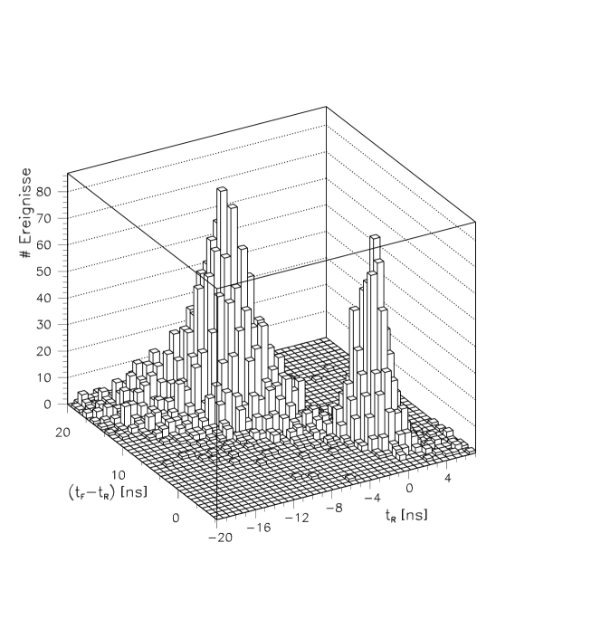
Fig. 16: The time measured in the rear part of the ZEUS calorimeter (RCAL) versus the difference in the times measured in the forward calorimeter (FCAL) and RCAL after the first level trigger. A clear separation can be seen between $ep$ interactions, which are centered on $(0,0)$ and beam-gas interactions.

The precise timing available from the ${}^{238}U$-scintillator calorimeter has been a particularly important tool for rejecting beam induced backgrounds occurring upstream of the IP, as well as other events which are asynchronous with the bunch crossing time (such as cosmic rays and noise). Figure 16 shows the $t_{RCAL}$ versus $t_{FCAL}-t_{RCAL}$ distribution, where events occurring upstream of the RCAL (giving $t_{FCAL}\approx 0$ ns, $t_{RCAL}\approx-10.5$ ns) are clearly displaced from the events occurring at the IP (with $t_{FCAL},t_{RCAL}\approx 0$ ns).

The H1 trigger has four levels. The first level trigger has a decision delay of $2.5$ $\mu$s, which determines the minimum pipeline length needed to store the full detector information. As with the ZEUS trigger, correlations between the information from different detectors are used to make the trigger decision. H1 uses four different types of pipelines:

• Fast RAM (e.g., for drift chambers);

• Digital shift registers (e.g., for systems readout with threshold discriminators);

• Analog delay lines (in the BEMC);

• Signal pulse shaping (in the LAr and TC, the pulse-shaping is adjusted in such a way that the maximum occurs at the time of the level one decision).

The second and third level triggers operate during the primary dead time of the readout. They work on the same data as the first level trigger, and must reach a decision within $20$ $\mu$s and $800$ $\mu$s, respectively. The first three levels of triggering should not exceed 1 kHz, 200 Hz and 50 Hz, respectively. (The second and third level trigger systems were not in use in the first years of data taking, such that the first level trigger had to be limited to a rate of about 50 Hz.)

The fourth level of triggering is based on full event reconstruction in MIPS R3000 based processor boards. Algorithms similar to the ones used for offline analysis are used to select valid events. The fourth level filter rejects about 70 % of the events, leading to a tape writing rate of about 15 Hz.

3.3 Kinematics specific to HERA

HERA collides $27.5$ GeV electrons or positrons on $820$ GeV protons. This leads to a center-of-mass energy squared

$$s = (k+P)^{2}$$ (46)

$$\approx 4E_{e}E_{p}$$ (47)

$$\approx (300\;\;{\rm GeV})^{2}$$ (48)

where $k$ and $P$ are the four-vectors of the incoming electron and proton, respectively. To get an equivalent center-of-mass energy in a fixed target experiment would require a lepton beam of energy $E_{lepton}=s/2m_{p}$, or $E_{lepton}=47$ TeV, which is about two orders of magnitude beyond what can be achieved today. It is therefore clear that HERA probes a very different kinematic regime to that seen by the fixed target experiments. For deeply inelastic scattering, the $Q^{2}$ range is extended to higher values by two orders of magnitude, while the range in the Bjorken-$x$ variable is increased by two orders of magnitude to smaller values for a fixed $Q^{2}$. This allows measurements of the proton structure at much smaller transverse and longitudinal distance scales.

The HERA experiments H1 and ZEUS have almost hermetic detectors. In the case of neutral current scattering, the kinematic variables can therefore be reconstructed from the electron, from the hadronic final state, or from a combination of the information from the electron and the hadrons. The different techniques used to date are described in section 3.4.

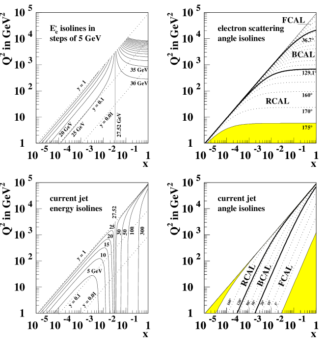
Fig. 17: Contour lines of fixed electron energy and angle, and fixed jet energy and angle in the ($x,Q^{2}$) plane. The labels FCAL, BCAL and RCAL refer to the different sections of the ZEUS calorimeter.

In neutral current DIS, the interaction can be thought of as electron-quark elastic scattering. The kinematics for DIS events are summarized in Fig. 17, where the contours of constant electron energy and angle, and scattered quark energy and angle are drawn on the kinematic plane. Most interactions involve small momentum transfers, and the electron is scattered at small angles. In small-$x$ events the hadronic final state is generally boosted in the electron direction, while for large-$x$ events the hadronic final state is in the proton direction. There is an extended region around $x=E_{e}/E_{p}(=0.03)$ where the scattered electron has an energy close to the electron beam energy. This region results in a “kinematic peak” in the electron energy spectrum, which is very useful for energy calibrations of the detectors.

Photoproduction is defined as the class of events where the square of the four-momentum transferred from the electron to the proton is very small (typically less than $10^{-2}$ GeV²). In this case, the electron is scattered at very small angles, and is not seen in the main detectors. It is in some cases tagged by special purpose electron taggers (see section 3.2). The exchanged gauge boson is then a quasi-real photon. The kinematical variables most relevant for photoproduction are the center-of-mass energy of the photon-proton system, $W$, and the transverse energy of the final state, $E_{T}$.

3.4 Kinematic variable reconstruction

3.4.1 Reconstruction of DIS variables

The relevant kinematics of DIS events are specified with two variables, as described in section 2.1. There are several possible choices for these two variables. Common choices are any two of ($x,y,Q^{2},W$). For the structure function measurements, the results are quoted in terms of $x$ and $Q^{2}$, while the natural variables to use for the total cross section measurement are $Q^{2}$ and $W$. The experiments measure the energy, $E_{e}^{\prime}$, and polar angle, $\theta_{e}$, of the scattered electron, and the longitudinal, $p_{z\;had}$ and transverse momentum of the hadronic final state, $p_{t\;had}$. There are many possible ways to combine these measurements and reconstruct the kinematical variables. We review some of these here.

• Electron Method:

  $$Q^{2} = 2E_{e}E_{e}^{\prime}(1+\cos\theta_{e})$$ (49)

  $$y = 1-\frac{E_{e}^{\prime}}{2E_{e}}(1-\cos\theta_{e})$$ (50)

  $$x = \frac{Q^{2}}{sy}$$ (51)

  This is the method which has historically been used in fixed target experiments. It is in many ways the easiest method, since it only requires the measurement of one particle. Its shortcomings are a seriously degraded $x$ resolution at small $y$ and large radiative corrections. The resolution is however very good at large $y$.

• Hadron Method:

  $$\delta_{had} = \sum_{i=1}^{\#hadrons}E_{i}(1-\cos\theta_{i})$$ (52)

  $$= E_{had}-p_{z\;had}$$ (53)

  $$y = \frac{\delta_{had}}{2E_{e}}$$ (54)

  $$Q^{2} = \frac{p_{t\;had}^{2}}{1-y}$$ (55)

  $$x = \frac{Q^{2}}{sy}$$ (56)

  This method relies entirely on the hadronic system, and also goes under the name Jacquet-Blondel method (?). The sum indicated for the measurement of $\delta_{had}$ runs over all final state hadrons. In practice, the final state hadrons are represented by tracks or calorimeter energy deposits. This method is stable against energy losses down the forward beam pipe since they contribute very little to $y$ or $p_{T}^{2}$. However, it is sensitive to calorimeter noise at very small $y$, and is sensitive to energy losses in the rear direction at higher values of $y$. It also requires a good understanding of energy scales and energy losses in inactive material. On the other hand, it is rather insensitive to radiative corrections.

• Double Angle Method:

  $$\cos\gamma = \frac{p_{t\;had}^{2}-\delta_{had}^{2}}{p_{t\;had}^{2}+\delta_{had}^{2}}$$ (57)

  $$Q^{2} = 4E_{e}^{2}\frac{\sin\gamma(1+\cos\theta_{e})}{\sin\gamma+\sin\theta_{e}-\sin(\theta_{e}+\gamma)}$$ (58)

  $$x = \frac{E_{e}}{E_{p}}\frac{\sin\gamma+\sin\theta_{e}+\sin(\theta_{e}+\gamma)}{\sin\gamma+\sin\theta_{e}-\sin(\theta_{e}+\gamma)}$$ (59)

  This method relies on the electron polar angle and the angle $\gamma$ which characterizes the hadronic final state (?). In a simple $eq\rightarrow eq$ picture with massless quarks, the angle $\gamma$ is the polar angle of the scattered quark. This reconstruction method has the advantage that it does not require precise knowledge of energy scales (variations in scale with polar angle will however distort the $\gamma$ measurement.) It also results in small radiative corrections. However, the resolution is poor if $y$ is very small.

• $\Sigma$–Method:

  $$y = \frac{\delta_{had}}{\delta}$$ (60)

  $$Q^{2} = \frac{E_{e}^{\prime 2}\sin^{2}\theta_{e}}{1-y}$$ (61)

  $$x = \frac{Q^{2}}{sy}$$ (62)

  This method (?) makes use of the longitudinal momentum conservation relation $E-P_{z}=2E_{e}$. The estimates of $E-P_{z}$ carried by the hadrons and electron respectively are $\delta_{had}$ and $\delta_{e}$, and $\delta=\delta_{e}+\delta_{had}$. At small $y$, $\delta\approx\delta_{e}$, and is rather well measured, whereas at large $y$ both $\delta_{had}$ and $\delta_{e}$ are important. $\delta_{had}$ suffers from significant energy losses (at the $15-20$ % level), and a wide distribution. The $\Sigma$–method corrects in part for this loss. The H1 collaboration has employed the $\Sigma$–method for $y<0.15$ in the measurement of $F_{2}$ from the 1994 data. For higher $y$, they have used the electron method. The $\Sigma$–method is rather insensitive to radiative corrections as it depends primarily on the hadronic variables.

• $P_{T}$ Method:

  $$Q^{2} = 4E_{e}^{2}\frac{\sin\gamma_{PT}(1+\cos\theta_{e})}{\sin\gamma_{PT}+\sin\theta_{e}-\sin(\theta_{e}+\gamma_{PT})}$$ (63)

  $$x = \frac{E_{e}}{E_{p}}\frac{\sin\gamma_{PT}+\sin\theta_{e}+\sin(\theta_{e}+\gamma_{PT})}{\sin\gamma_{PT}+\sin\theta_{e}-\sin(\theta_{e}+\gamma_{PT})}$$ (64)

  The $P_{T}$ method (?) was developed by ZEUS in the analysis of the 1994 data. The double-angle equations are used to calculate the kinematic variables, but with an improved estimate of the hadronic angle $\gamma$. This estimate makes use of the $p_{T}$ balance in NC DIS events, whence its name. The $p_{T}$ measured by the electron is used in the calculation of $\gamma$. It is also used to improve the measurement of $\delta_{had}$, as is longitudinal momentum balance in the form of the $\Sigma$–method. The ZEUS collaboration has employed the $P_{T}$ method over the full kinematic range for the extraction of $F_{2}$ in the 1994 data.

3.4.2 Reconstruction of photoproduction variables

The primary variable used in photoproduction is the hadronic center-of-mass energy $W$. In tagged photoproduction, this is calculated from the energy of the scattered electron:

$$W^{2}\approx sy\approx s(1-E_{e}^{\prime}/E_{e})\;\;\;.$$ (65)

The resolution is then given by the resolution of the electron calorimeters, which is typically $\sigma_{E}(GeV)\approx 0.25\cdot\sqrt{E(GeV)}$. The energy scale is very well known as it is calibrated using Bremsstrahlung events.

In untagged events, the hadronic measurement of $y$ described above must be used. This has much poorer resolution and has systematic shifts. It requires good knowledge of the hadronic energy scale as well as a detailed understanding of the noise.

Jet transverse energies are needed for measurements in hard photoproduction. These require a precise knowledge of the hadronic energy scale as well as energy losses resulting from inactive material. Energy smearing from the jet finding algorithm are also important. Typical jet energy resolutions are $\sigma_{E}(GeV)\approx 1.0\cdot\sqrt{E(GeV)}$. Uncorrected energies are about $20$ % too low, and are corrected using Monte Carlo methods.

3.4.3 Reconstruction of variables for exclusive final states

The standard kinematical variables are often much better reconstructed in exclusive processes, where in some cases the final state is known and energy-momentum conservation can be used effectively. An example is vector meson production ($ep\rightarrow epV$), described in section 7, where the vector meson $V$ is reconstructed with the tracking detectors (e.g., $\rho^{0}\rightarrow\pi^{+}\pi^{-}$). In this case, $y$ can be reconstructed using the hadronic method described above, using the measured energies and momenta, to high accuracy. In DIS, the electron energy is then constrained if the scattering angle is known, via:

$$E_{e}^{\prime}=\frac{2E_{e}-\delta_{had}}{1-\cos\theta_{e}}\;\;\;.$$ (66)

In this case, the kinematic variables are reconstructed to an accuracy of a few %. Many other kinematic variables are needed to fully describe the exclusive processes. These include the mass of the final hadronic state (excluding the proton), the square of the four-momentum transfer at the proton vertex, $t$, and various decay angles. These will be described in more detail as they become relevant.

3.5 Coverage of the phase space

3.5.1 Phase space coverage in DIS

The HERA measurements in DIS cover a vast kinematic range, as shown in Fig. 4. For example, the measurements of $F_{2}$ with the 1995 data sets extend down to $Q^{2}$ values of $0.1$ GeV² and up to $Q^{2}=5000$ GeV². For each $Q^{2}$, typically two orders of magnitude are covered in $x$: from $10^{-5}\rightarrow 10^{-3}$ at the lowest $Q^{2}$ to $10^{-2}\rightarrow 0.3$ at $Q^{2}=500$ GeV². The region at large $y$ requires very efficient and pure electron finding algorithms down to the lowest possible energies, while the small-$y$, or large-$x$, region requires a precise understanding of the hadronic final state. Both collaborations have invested tremendous efforts in developing analysis tools which could work in these extreme regions and thus allow measurements over such a large kinematic range. The measurement of $F_{2}$ requires that the cross section be measured in bins of $x$ and $Q^{2}$. At the highest values of $Q^{2}$, the measurements are limited by lack of event statistics. It is possible to measure a single differential cross section $d\sigma/dQ^{2}$ up to $Q^{2}$ values of $40,000$ GeV², for both neutral and charged current events. This allows a measurement of the $W$ mass, as well as searches for exotic phenomena.

The main detectors of ZEUS and H1 were optimized primarily for the large $Q^{2}$ region of phase space. At the lower values of $Q^{2}$, various detector improvement programs have enhanced the kinematical coverage. The original calorimeter designs allowed the measurement of DIS NC events down to $Q^{2}\approx 4$ GeV² (with the vertex at $\overline{Z}\approx 0$ cm). In order to probe the transition region between photoproduction and DIS, the calorimeters had to be modified or enhanced by new devices. These include a new rear calorimeter for the H1 experiment (?) which not only has higher precision than the BEMC, but also begins at a distance of $4$ cm from the beam, as opposed to $\approx 10$ cm. This detector was installed in the 1994-1995 winter shutdown. The ZEUS collaboration added a small angle electron calorimeter, the Beam Pipe Calorimeter (BPC), in the shutdown period 1994-1995 to access the $Q^{2}$ range $0.1\rightarrow 1$ GeV². In addition, the central modules of the Uranium-scintillator calorimeter were moved to within $4$ cm of the beam to reach down to $Q^{2}$ values of $1$ GeV².

In addition to the modifications to the detectors, the kinematic range covered was extended by several techniques.

1. Using data with a shifted vertex. The angular coverage of the detectors extends to smaller values of the electron scattering angles as the vertex is moved away from the rear calorimeters. The shifted vertex events were produced via dedicated HERA runs in which the primary vertex was moved to $\overline{Z}\approx+80$ cm. These runs were used by ZEUS and H1 to measure down to $Q^{2}=0.4$ GeV² with their main detectors. In addition, H1 used events from the standard running ($\overline{Z}\approx 0$ cm) in the $+Z$ tail of the vertex distribution. A significant number of events are present at $Z\approx 80$ cm which result from protons in neighboring RF bunches. These events access the same $Q^{2}$ range as the shifted vertex runs, but have larger normalization uncertainties.

2. Using data with hard initial state radiation. A large fraction ($\approx 30$ %) of the photons from events with hard initial state radiation are measured in the photon calorimeters of the luminosity system. The resultant $ep$ collisions therefore occur at lower center-of-mass energies, and lower $Q^{2}$ values can be attained. This method was employed both by the ZEUS and H1 experiments.

3.5.2 Phase space coverage in photoproduction

Photoproduction events at HERA are very small $Q^{2}$ events where the scattered electron is either measured by an electron calorimeter near the electron beamline, or are antitagged as DIS via the absence of an electron in the main detectors. These two techniques allow very different coverage of the phase space. We consider each in turn.

Tagged photoproduction

In addition to the main calorimeter, the ZEUS detector currently has electron calorimeters positioned at $Z=-8,-35$, and, $-44$ m. These calorimeters are placed very close to the beamline, and are positioned after magnets of the HERA accelerator. They require that the electron scattering angle be very small, and analyze different regions of the electron energy spectrum. E.g., the $35$ m tagger limits $Q^{2}<10^{-2}$ GeV², and measures electrons in the energy range $5<E<18$ GeV, corresponding to a $W$ range $180<W<270$ GeV. The recently added $8$ and $44$ m taggers cover higher and lower $W$ ranges, respectively, as shown in Fig. 18. The H1 experiment currently has taggers at $Z=33,44$ m and is planning a tagger at $Z=8$ m. These cover essentially the same kinematic range as the ZEUS detectors.

Fig. 18: The $W$ range tagged by the different electron calorimeters located along the electron beamline of the ZEUS detector. The $8$-m tagger tags photons at the large $W$ range, the $35$-m tagger tags the intermediate $W$ range, and the $44$-m tagger tags the small $W$ range. The open histogram shows the $W$ distribution of all photoproduction events.

Untagged photoproduction

It is also possible to tag photoproduction by requiring the absence of the scattered electron in the main detector. This limits $Q^{2}<4$ GeV² ($Q^{2}<1$ GeV² as of the 1995 data sets). The median $Q^{2}$ depends on the process studied, but is typically $10^{-5}$ GeV² (?). This method allows measurements over a much wider range of $W$. However, it requires that $W$ be measured from the hadronic system in the main detector which has much lower precision than determining it directly from the scattered electron.

3.5.3 Phase space coverage in the forward direction

Many of the physics results coming from HERA in the first years of operation deal with diffraction ($ep\rightarrow epX$, viewed as photon diffraction on the proton). Ideally, this physics would be done solely with events where the scattered proton is tagged. Both ZEUS and H1 have leading proton spectrometers, with high acceptance (for the ZEUS LPS) in the proton elastic peak, $x_{l}=1$, for $0.2<p_{T}<0.6$ GeV. The overall acceptance for elastic photoproduction of $\rho^{0}$ mesons is about $6$ %.

The acceptance of the leading proton spectrometers is quite small, and it is therefore profitable to also study diffraction with the other detector components. There are different techniques for doing this (see section 6). The most important detector parameter is the rapidity coverage of the forward calorimeters and tagging devices. Forward rapidity coverage is needed both for the reconstruction of large mass diffractive final states as well as for rejecting backgrounds.

The ZEUS Uranium-scintillator forward calorimeter extends to within $10$ cm of the beam and begins at $Z=2.2$ m, which implies a rapidity cutoff near $\eta=4$. Additional information is available from the proton remnant tagger (PRT), which has scintillator planes located at $Z=5$ m and $Z=22$ m. The PRT allows the tagging of charged particles in the rapidity intervals $4<\eta<7$.

The H1 LAr calorimeter extends to $\eta\approx 3.7$. This is complemented by the forward plug calorimeter, FPC, with coverage $3.5<\eta<5.5$. Collimators are placed between the interaction point and the FPC. This implies a minimum energy cutoff for particles to reach the FPC. However, the scattering and showering produced by the collimator can be used to advantage. The forward muon chamber is sensitive to charged particles from these processes. The resulting coverage of the H1 detector is $5.0<\eta<6.5$. The H1 PRT covers the region $6.0<\eta<7.5$.

3.6 Radiative corrections

To compare measured cross sections with theoretical calculations it is necessary to include the effects of QED radiative processes. This is typically done by correcting the measured cross sections for these effects, either by using event simulation packages which include radiative effects, or from analytical calculations. The difference between the radiative cross sections and the Born cross sections are used to apply correction factors.

Fig. 19: Diagrams showing the different LO QED corrections to the Born diagram.

First order QED radiative processes from the electron are shown in Fig. 19. They include initial state radiation (ISR), final state radiation (FSR) and virtual loop corrections. There are also radiative effects for the proton, or quarks. These are typically not corrected, and the measured structure functions therefore include QED radiation.

For ISR, the energy of the incoming electron is effectively lowered. The apparent $x$ and $Q^{2}$ calculated with the electron variables are no longer the same as the propagator $x$ and $Q^{2}$. QED radiation therefore causes shifts in the mean reconstructed kinematic variables. The shifts depend on the choice of reconstruction method. Methods relying more on the hadronic system typically suffer smaller shifts. Note that the bulk of the radiated photons are collinear with the incoming electron. They can therefore be measured by the photon calorimeters of the luminosity systems from ZEUS and H1. Measuring this spectrum is a very good check that ISR is simulated correctly. FSR is also typically collinear, with the outgoing photon at small angles to the scattered electron. These are usually not distinguished as separate clusters by the calorimeters, and therefore do not results in shifts in the reconstructed kinematic variables. However, there is a tail to larger opening angles, which will produce shifts in the kinematic variables if not correctly simulated. These effects are best studied with Monte Carlo event simulations which take QED radiation into account. In the Monte Carlo program HERACLES (?; ?), the 4–momentum of the radiative photon is sampled according to the 5–fold differential cross section for radiative photon emission $d\sigma/dxdydE_{\gamma}d\theta_{\gamma}d\phi_{\gamma}$ from the electron and is saved together with the other stable particles. These are then traced through the detector.

The shift of the apparent variables from the true depends strongly on the reconstruction method chosen for the kinematic variables. The shift can be effectively limited by appropriate event selection cuts. For example, requiring $\delta>0.7(2E_{e})$ limits the maximum ISR photon energy to $E_{\gamma}<0.3E_{e}$, which in turn limits the amount of shift possible in the reconstruction of the kinematic variables. Note that the correction to the measured cross section is typically highest at large $y$, as this corresponds to small scattered electron energy.

In addition to producing measured kinematic variables which are shifted from the propagator values, QED radiation also changes the cross section for a given $x$ and $Q^{2}$. The cross section must therefore also be corrected to the Born level (no QED radiation). These corrections are typically small, since the QED coupling constant appears, and can usually be treated as a multiplicative correction. For example, the differential cross section for NC DIS can be approximated as

$$\frac{d^{2}\sigma^{NC}}{dxdQ^{2}}=\frac{d^{2}\sigma^{Born}}{dxdQ^{2}}(1+\delta^{r}(x,Q^{2}))\;\;\;.$$ (67)

3.7 Event modeling and unfolding of detector effects

Detailed Monte Carlo simulations are indispensable for the extraction of physical quantities from the measurements. The use of Monte Carlo event simulators was already mentioned in the previous section for the study of QED radiative effects. Monte Carlo simulations are also used to correct for limited geometrical acceptance of the detectors and to understand the effects of the measurement resolution on kinematical variables.

Monte Carlo simulations can also be used to study the relationship between measured quantities and the physically fundamental quantities. An example of this is the relation between the jets measured at the detector level and the partons which originally produced the jets.

Monte Carlo event simulations are used extensively in developing the data selection cuts. The Monte Carlo programs can help determine which variables are particularly useful for separating signal from background. They also indicate where certain variables are measured accurately, and where they are not well measured. In developing the cuts and determining the acceptance corrections, it is necessary that the Monte Carlo simulations accurately describe the data. In practice, this means that many different Monte Carlo programs must be used, each tuned for a specific class of processes. It also means that detailed simulations of the detector apparatus must be performed, including inactive as well as active materials.

We describe briefly a few of the more commonly used event generators for DIS and photoproduction. The many special purpose generators, e.g. for diffractive processes or exotic processes, are beyond the scope of this report. We finish this section with a brief description of the detector simulation packages.

3.7.1 Generators for DIS

Several generators are used together to describe DIS events at HERA. The program HERACLES (?; ?) is used to simulate the effects of electroweak radiation from the electron and quark. HERACLES is interfaced with either ARIADNE (?; ?), HERWIG (?) or LEPTO (?) for the simulation of the hard scattering and the simulation of the initial and final QCD radiation from the partons. ARIADNE is based on the color dipole model (?), where the struck quark-diquark system act as a radiating color antenna. In the program HERWIG, coherent parton showers are produced which form color neutral clusters, while the LEPTO package produces parton showers according to the DGLAP evolution equation. Perturbative QCD corrections are implemented by taking into account the full ${\mathcal{O}}(\alpha_{s})$ or ${\mathcal{O}}(\alpha_{s}^{2})$ matrix elements. In the case of ARIADNE and LEPTO, the program package JETSET (?) is then used for the fragmentation of the resulting partons into hadrons, and for their decay. JETSET is based on the Lund string model of fragmentation (?). These programs are under constant revision as new data become available, and different versions are used for different analyses.

3.7.2 Generators for photoproduction

The two principal generators used to simulate photoproduction reactions are the PYTHIA program (?) and the HERWIG program (?). PYTHIA is a Lund type Monte Carlo program. It allows for both resolved as well as direct photon reactions. The program allows for both initial as well as final state QCD radiation, and uses the JETSET package for hadronization. The hard scattering cross sections are simulated in LO. The H1 collaboration has also made extensive use of the PHOJET generator (?; ?).

3.7.3 Detector simulation

The output of the event generation step is fed into the detector simulation programs. These are based on the GEANT (?) package which is in common use in high energy physics experiments. Detailed simulation of the geometry and materials of the detector are performed, and the output of the programs are compared with measurements from test beams as well as from $ep$ interaction data. The individual programs used by the ZEUS and H1 experiments represent enormous efforts. They are constantly being refined to give the best possible reproduction of the response of the detector.

4 Inclusive cross section measurements

Inclusive cross section measurements are of fundamental importance. Considerable debate on the behavior of the $ep$ cross section at high center-of-mass energies was fueled in the late 1980’s and early 1990’s by the approaching turn-on of HERA. In $e^{+}e^{-}$ scattering, the total cross section as a function of the center-of-mass energy is calculable in electroweak theory, and the measurements are in excellent agreement with the predictions. The behavior of the hadron-hadron scattering cross sections as a function of the center-of-mass energy are not calculable since they depend on the structure of the hadrons. However, cross sections have been measured for many different combinations of hadrons (proton-proton, proton-antiproton, proton-pion, …). It was found experimentally that these cross sections all have a similar energy dependence at high energies (?), given by

$$\sigma\sim s^{0.08}\,,$$ (68)

where $s$ is the hadron-hadron center-of-mass energy. What would the data show in the case of $ep$ scattering ?

Two different regimes are generally differentiated:

1. The small $Q^{2}$ regime, where electron-proton scattering proceeds via photon exchange. When $Q^{2}\rightarrow 0$, the photon is almost real, and we can consider the scattering as photon-proton scattering. The transverse distance scale defined by $Q^{2}$ is much larger than the size of the proton, so that the details of the proton structure are not expected to be important for the total cross section. It has been known for some time that photoproduction can be viewed as hadron-hadron scattering, where the photon has fluctuated into a vector meson. It was therefore expected that the cross section at $Q^{2}\approx 0$ would have a similar behavior to the hadron-hadron scattering cross sections.

2. The deep inelastic scattering regime (DIS), where electron-proton scattering proceeds via $\gamma,Z\;\rm{or}\;W$ exchange (photon exchange dominates until $Q^{2}\approx M_{Z,W}^{2}$). In this case, the transverse distances probed in the interaction are a fraction of the proton radius, and the cross section will depend on the details of the proton structure. No experimental data existed pre-HERA for center-of-mass energies of the exchanged boson-proton system larger than about $25$ GeV. Many different predictions existed for the behavior of the cross section, ranging from a small energy dependence similar to that seen in hadron-hadron scattering (?) to a very steep energy dependence (?; ?; ?). The measurement of this cross section (or equivalently $F_{2}$) is one of the most exciting results to come from HERA.

In the following sections, we first describe the measurements of the $\gamma p$ and $\gamma^{*}p$ cross section at HERA. We then describe the structure function measurements and discuss the results.

4.1 Total photoproduction cross section

Fig. 20: The total cross section measured in hadronic scattering as a function of the center-of-mass energy for $pp,\;p\overline{p},\;\pi^{+}p,\;\pi^{-}p$ scattering. The cross sections show a universal rise at high energies of the form $\sigma\sim s^{0.08}$ (?).

As mentioned above, the total hadronic cross sections rise with center-of-mass energy in a universal way. The energy dependence for $\overline{p}p,pp,\pi^{-}p,\rm{and}\;\pi^{+}p$ scattering is shown in Fig. 20. The solid lines shown in the figure are fits which include a component dying rapidly with $s$, the center-of-mass energy, and a second component which persists at high energies (?). The second component was found to be universal, with the cross sections rising as $s^{0.08}$. The corresponding measurements for $\gamma p$ scattering only extended to $\gamma p$ center-of-mass energies of about $25$ GeV before the advent of HERA, and the high energy dependence was therefore not well known. Predictions based on perturbative QCD varied widely, from a soft energy dependence to a very steep energy dependence (?; ?; ?; ?; ?).

4.1.1 From $ep$ scattering to $\gamma p$ scattering

In the Standard Model, the reaction $ep\rightarrow eX$ can proceed via $\gamma$ or $Z^{0}$ exchange. At small enough $Q^{2}$, $Z^{0}$ exchange can be neglected. Furthermore, we can decompose the cross section into a term representing the flux of photons from the electron, and a term representing the photon-proton scattering process. This is depicted schematically in Fig. 7. The differential cross section can then be written in the form

$$\frac{d^{2}\sigma(ep)}{dWdQ^{2}}=\Gamma(\sigma_{T}^{\gamma p}+\epsilon\sigma_{L}^{\gamma p})\;,$$ (69)

where $\Gamma$ represents the flux factor of virtual photons, $\sigma_{T},\sigma_{L}$ are the absorption cross sections for transverse and longitudinally polarized photons, and $\epsilon$ is the ratio of the flux for longitudinal to transverse photons.

If we restrict ourselves to photoproduction, $Q^{2}\approx 0$, then the photon is transversely polarized and only the first term in the cross section expression will contribute. Given that the flux factor $\Gamma$ is known (see discussion in section 2.4), a measurement of the differential $ep$ cross section allows the extraction of the total photoproduction cross section.

4.1.2 Measurements at HERA

The measurements at HERA rely on the electron calorimeters described in section 3.5.2. These detectors measure the scattered electrons in the energy range $10-22$ GeV, which corresponds to a $W$ range $150-250$ GeV. Observing the electron in these detectors limits $Q^{2}$ to a maximum of $0.02$ GeV². Loose requirements were placed on the energy seen in the main detectors. Even so, the acceptance depends crucially on the detailed composition of the hadronic final state, so that acceptance corrections relied heavily on Monte Carlo programs. The results from ZEUS (?), $\sigma_{tot}=143\pm 4\pm 17$ $\mu$b, and H1 (?), $\sigma_{tot}=165\pm 2\pm 11$ $\mu$b, are shown in Fig. 21. The expectations based on the energy dependence measured in hadronic interactions are in good agreement with the HERA results, confirming the hadronic behavior of real photons.

Fig. 21: The dependence of the total photoproduction cross section as a function of the $\gamma p$ center-of-mass energy, $W$. The HERA results are compatible with an extrapolation of the low energy measurements using the energy dependence found from hadronic scattering, indicating that the photon behaves similarly to a hadron. The curves are from ? with $\alpha_{0}=1.08$ and $\alpha_{0}=1.11$ and from the ALLM parameterization (?).

4.2 Total DIS cross section

The measurements of the total photoproduction cross section can be extended to higher $Q^{2}$, where a virtual photon (or weak boson) is involved. There are several important differences to consider once the virtuality increases:

• The photon can acquire a longitudinal polarization, so that both the transverse as well as the longitudinal cross sections are important.

• The flux of virtual photons is not uniquely defined, and requires a convention. The Hand convention is normally chosen (see Eq. (24)).

• The photon probes smaller transverse distances. The transverse distance scale probed is given by

  $$d\approx\frac{0.2}{Q({\rm GeV})}\;{\rm fm}\;\;\;.$$ (70)

  For $Q^{2}>1$ GeV², transverse distances at the level of a fraction of the proton radius are probed.

  The longitudinal distances over which the photon fluctuations occur depend on $1/x$, as described in section 2.8.

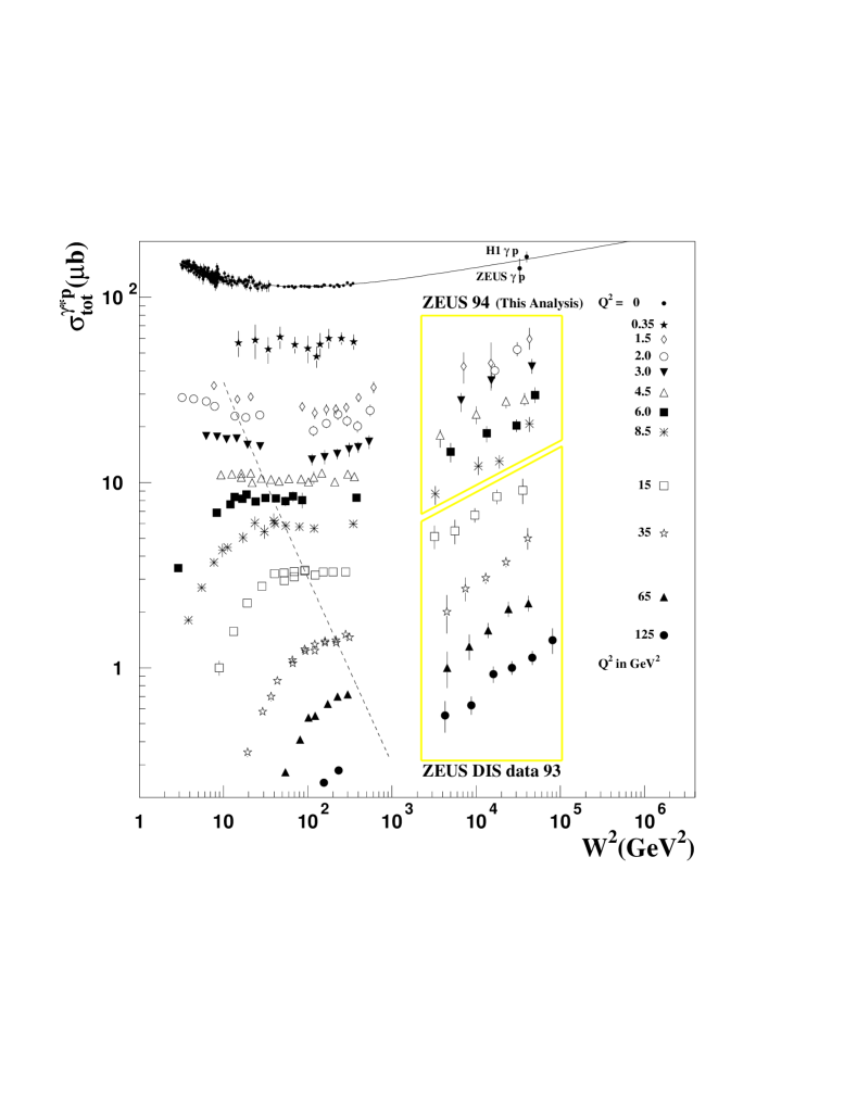
Fig. 22: The $\gamma^{*}p$ cross section versus $W^{2}$ for small $Q^{2}$ data from the ?. The data are compared to results from fixed target experiments as well as to the photoproduction results shown in the previous figure.

The total $\gamma^{*}p$ cross sections are extracted from the measured values of $F_{2}$ (discussed in the next sections) using equation 23. They are given as a function of $W^{2}$ in Fig. 22 for $Q^{2}$ values in the range $1.5<Q^{2}<125$ GeV², and are compared with the photoproduction results as well as with results from fixed target experiments. As can be seen clearly in this figure, the DIS cross section has a $W^{2}$ dependence which is considerably steeper at large $W^{2}$ than that found in photoproduction. The $W^{2}$ dependence is also seen to vary strongly with $Q^{2}$. The region to the right of the dashed line corresponds to $x<0.1$, where the photon lifetime, in the proton rest frame, is large enough so that it typically survives for distances larger than the proton radius (see section 2.8).

The rise of the cross section with energy, for a fixed $Q^{2}$, is expected to come to an end at some $W^{2}$, in analogy with the Froissart bound for hadron-hadron scattering (?):

$$\sigma_{tot}\leq C\ln^{2}\frac{s}{s_{0}}\;\;.$$ (71)

The form of this bound is not known precisely in DIS (?), but it is expected that there is some analogous limit. The present HERA data show no signs of a flattening of the cross section at large $W$, indicating that unitarity constraints do not play a strong role in the kinematic region presently probed.

In a geometrical picture of the interaction, the constituents of the proton are viewed as being resolved into sub-constituents as the transverse and longitudinal distance scales are reduced. A schematic representation of this effect is shown in Fig. 5. In this picture, all the structure is assigned to the proton. The structure can also be thought of as belonging to the photon, as discussed in section 2.8. In the proton rest frame, the photon has a long lifetime, and can fluctuate into a quark-antiquark pair, and perhaps develop further hadronic structure, before scattering from the proton. In this case, the scattering cross section is increased because of the increased flux of partons from the photon scattering off the proton.

4.3 HERA structure functions

We now discuss the measured cross sections from the perspective of proton structure functions. As has been discussed in section 2.1, the collider kinematics allow to reach much larger values of $Q^{2}$ and smaller values of $x$. The measurements from fixed target experiments are limited to $x>0.01$ for $Q^{2}>10$ GeV², and therefore do not probe the very small values of $x$ in the regime of perturbative QCD. However, the measurements from the fixed target experiments fix the valence quark densities, and constrain the form of the sea quark and gluon densities for $x\geq 0.01$. The HERA measurements probe similar regions of $x$, but at much larger $Q^{2}$, thereby testing the $Q^{2}$ evolution of the structure functions. They also probe much smaller values of $x$ for a fixed $Q^{2}$, thereby allowing precise measurements on the behavior of the parton densities for very small proton momentum fraction. The behavior of the parton densities for $x<0.01$ is of great theoretical interest, and could lead the way to a better understanding of perturbative QCD. It is expected that parton densities become large at small $x$, while the coupling strength, $\alpha_{s}$ remains small, representing a new physical situation for QCD calculations. As was discussed in section 2.3, there are different approaches to the perturbative solution of QCD leading to different predictions on the behavior of the structure function at small $x$ (NLO DGLAP versus LO BFKL).

In the following sections, we first review the definition of the structure functions and the expectations pre-HERA. We then describe how the structure function measurements are performed at HERA, and discuss the results. Finally, the methods used to extract the gluon density in the proton are described.

A comprehensive review of structure functions has recently been published by ?.

4.3.1 Structure functions in neutral and charged current scattering

Neutral current cross sections

The differential cross section for $e^{-}p$ neutral current (NC) scattering is conventionally written in terms of the NC structure functions $F_{2},\;F_{L}$ and $F_{3}$ as shown in Eq. (6). We rewrite the cross section here and discuss explicitly the dependence on polarization.

$$\frac{d^{2}\sigma^{e^{-}p}}{dxdQ^{2}}=\frac{2\pi\alpha^{2}}{xQ^{4}}\left[Y_{+}F_{2}^{L,R}(x,Q^{2})-y^{2}F_{L}^{L,R}(x,Q^{2})+Y_{-}xF_{3}^{L,R}(x,Q^{2})\right]\;,$$ (72)

with $x$ and $Q^{2}$ defined at the vector boson-quark vertex. Note that the structure functions are process dependent. For example, one has to make the replacement $F_{3}^{L,R}\rightarrow-F_{3}^{R,L}$ for $e^{+}p$ scattering, where $L,R$ represent the polarization of the lepton beam. The parity-violating $xF_{3}$ term is only important at large $x$ and $Q^{2}$ where it substantially reduces the $e^{+}p$ cross section, while increasing the cross section for $e^{-}p$ scattering. The contribution from $F_{L}$ is important at large $y$ and small $x$. It is expected to be negligible at large $x$ and $Q^{2}$. The structure functions depend on the lepton beam polarization as described below. We assume here that the proton beam is unpolarized.

The explicit $y$ dependence, which is due to the helicity dependence of electroweak interactions, is contained in the functions

$$Y_{\pm}(y)=1\pm(1-y)^{2}\ \;,$$ (73)

with $y$ related to the electron scattering angle in the $eq$ rest frame, $\theta^{*}$, as

$$y=\frac{1-cos\theta^{*}}{2}\;.$$ (74)

The dependence on the quark structure of the proton, and on the $Z^{0}$ propagator, is absorbed in the structure functions. To LO, these are

$$\left(\begin{array}[]{c}F_{2}^{L,R}(x,Q^{2})\\ xF_{3}^{L,R}(x,Q^{2})\end{array}\right)=x\sum_{q={\rm quarks}}\left(\begin{array}[]{c}C_{2}^{q\;L,R}(Q^{2})[q(x,Q^{2})+\overline{q}(x,Q^{2})]\\ C_{3}^{q\;L,R}(Q^{2})[q(x,Q^{2})-\overline{q}(x,Q^{2})]\end{array}\right)$$ (75)

written in terms of the quark densities in the proton ($q=u,\;d,\;c,\;s,\;t,\;b$) and the corresponding antiquark densities $\overline{q}$. The structure function $F_{L}$ is discussed in section 4.3.7.

The $Q^{2}$ dependent coefficient functions, $C_{2}^{q}$ and $C_{3}^{q}$, are given in terms of the vector and axial vector couplings

$$C_{2}^{q\;L,R}(Q^{2}) = |V_{q}^{L,R}|^{2}+|A_{q}^{L,R}|^{2}\;,$$ (76)

$$C_{3}^{q\;L,R}(Q^{2}) = \pm 2V_{q}^{L,R}A_{q}^{L,R}\;,$$ (77)

which depend on the polarization of the $e^{\pm}$ beam ($L=+,R=-$)

$$\begin{array}[]{rrll}V_{q}^{L,R}=&e_{q}&+&e_{e}(v_{e}\pm a_{e})v_{q}\chi_{Z}\;,\\ A_{q}^{L,R}=&&&e_{e}(v_{e}\pm a_{e})a_{q}\chi_{Z}\;.\end{array}$$ (78)

Expanding the expressions for $C_{2},C_{3}$ yields

$$\begin{array}[]{rrll}C_{2}^{q}(Q^{2})=&e_{q}^{2}&+&2e_{e}e_{q}v_{q}(v_{e}+Pa_{e})\chi_{Z}+(v_{q}^{2}+a_{q}^{2})(v_{e}^{2}+a_{e}^{2}+2v_{e}a_{e}P)\chi_{Z}^{2}\;,\\ C_{3}^{q}(Q^{2})=&&&2e_{e}e_{q}a_{q}(a_{e}+Pv_{e})\chi_{Z}+e_{e}^{2}(2v_{q}a_{q})(2v_{e}a_{e}+Pv_{e}^{2}+Pa_{e}^{2})\chi_{Z}^{2}\;,\end{array}$$ (79)

where $e_{e}$ is the charge of the electron ($-1$) and $e_{q}$ is the quark charge in units of the positron charge. Note that the charge does not change signs for antiparticles (e.g., $e_{e}=-1$ for positrons, and $e_{\bar{u}}=2/3$). $P$ is the degree of left-handed longitudinal polarization,

$$P=\frac{N_{L}-N_{R}}{N_{L}+N_{R}}\;,$$ (80)

where $N_{L},\;N_{R}$ are the number of left-handed and right-handed electrons (or positrons). The vector and axial vector coupling of the fermion are given by

$$\begin{array}[]{rcl}v_{f}&=&(T_{3}^{f}-2e_{f}\sin^{2}\theta_{w})\;,\\ a_{f}&=&T_{3}^{f}\;,\end{array}$$ (81)

with $\theta_{w}$ the weak mixing angle, $T_{3}^{f}$ the third component of the weak isospin and $e_{f}$ the electric charge in units of the positron charge. The factor $\chi_{Z}$ is given by

$$\chi_{Z}=\frac{1}{4\sin^{2}\theta_{w}\cos^{2}\theta_{w}}\frac{Q^{2}}{Q^{2}+M_{Z}^{2}}\;.$$ (82)

where $M_{Z}$ is the $Z^{0}$ mass. All relevant electroweak parameters have been measured to high precision (?).

For $Q^{2}\ll M_{Z}^{2}$, the structure functions in LO reduce to

$$\left(\begin{array}[]{c}F_{2}(x,Q^{2})\\ xF_{3}(x,Q^{2})\end{array}\right)=x\sum_{q={\rm quarks}}\left(\begin{array}[]{c}e_{q}^{2}[q(x,Q^{2})+\overline{q}(x,Q^{2})]\\ 0\end{array}\right)\;.$$ (83)

Charged current cross sections

The differential cross section for $e^{\pm}p$ charged current (CC) scattering can be written in terms of the of the CC structure functions $F_{2},\;F_{L}$ and $F_{3}$ as

$$\frac{d^{2}\sigma^{e^{\pm}p}}{dxdQ^{2}}=\frac{G_{F}^{2}}{4\pi x}\left(\frac{M_{W}^{2}}{Q^{2}+M_{W}^{2}}\right)^{2}\left[Y_{+}F_{2}(x,Q^{2})-y^{2}F_{L}(x,Q^{2})\mp Y_{-}xF_{3}(x,Q^{2})\right]\;\;.$$ (84)

The Fermi constant, $G_{F}$, can be expressed as

$$G_{F}=\frac{\pi\alpha}{\sqrt{2}\sin^{2}\theta_{W}M_{W}^{2}}\;,$$ (85)

with $M_{W}$ the mass of the $W^{\pm}$.

As in the NC case, the parity-violating $xF_{3}$ term substantially reduces the $e^{+}p$ cross section at large $Q^{2}$, while increasing the cross section for $e^{-}p$ scattering. The contribution from $F_{L}$ is expected to be negligible and is ignored. In LO pQCD, we can specify the quark flavors which enter into the scattering. For $e^{-}p$ scattering, and left-handed electron polarization,

$$F_{2} = 2x\left[u(x,Q^{2})+c(x,Q^{2})+\bar{d}(x,Q^{2})+\bar{s}(x,Q^{2})\right]\;,$$ (86)

$$xF_{3} = 2x\left[u(x,Q^{2})+c(x,Q^{2})-\bar{d}(x,Q^{2})-\bar{s}(x,Q^{2})\right]\;,$$ (87)

while $F_{2}=xF_{3}=0$ for right-handed electron polarization. For $e^{+}p$ scattering, and right-handed positron polarization,

$$F_{2} = 2x\left[d(x,Q^{2})+s(x,Q^{2})+\bar{u}(x,Q^{2})+\bar{c}(x,Q^{2})\right]\;,$$ (88)

$$xF_{3} = 2x\left[d(x,Q^{2})+s(x,Q^{2})-\bar{u}(x,Q^{2})-\bar{c}(x,Q^{2})\right]\;,$$ (89)

while $F_{2}=xF_{3}=0$ for left-handed positron polarization.

4.3.2 Pre-HERA expectations

It is interesting to review the pre-HERA expectations for the structure functions. These expectations are summarized in the proceedings of the ‘Physics at HERA’ workshop from 1991 (?). We focus on the expectations for the neutral current structure function $F_{2}$. Most of the initial speculation concerned the behavior of the parton densities at small $x$, and the consequences of the anticipated rise of $F_{2}$ with decreasing $x$.

$F_{2}$ at small $x$

It was widely believed that $F_{2}$ would rise with decreasing $x$ in the HERA regime, as this is a consequence of both the DGLAP and BFKL evolution equations. However, this view was not universally held. Some authors expected the structure function to remain rather flat with decreasing $x$ (?), in contrast to BFKL inspired approaches which predicted a steep rise of the form $x^{-0.5}$ at small $x$ (as discussed in section 2.6). Parton density parameterizations existed with a range of possible $F_{2}$ behaviors within these limits (?; ?; ?; ?; ?). One group of authors, Glück, Reya and Vogt (GRV), predicted a steep rise of $F_{2}$ due purely to QCD radiative processes. They parameterized the parton densities as essentially valence like at a very small scale $Q_{0}^{2}=0.34$ GeV², and predicted $F_{2}$ at larger values of $Q^{2}$ using NLO DGLAP evolution. I.e., they assumed $F_{2}$ was calculable from pQCD with valence-like parton densities defined at a much smaller scale than that used by other authors.

Saturation at small $x$

The question of the validity of the DGLAP evolution at small $x$ was widely discussed. One issue was whether the BFKL evolution, which is based on an expansion in $\ln(1/x)$, was more appropriate at small $x$. A perhaps more fundamental issue was whether the standard evolution equations based on parton splitting would be valid at all, or whether parton recombination would play a role at high parton densities. ? suggested that such effects could be represented by nonlinear terms in the evolution equations. The result would be a ‘saturation’ of the parton densities at small $x$. It was expected that these saturation effects would be seen at HERA (see, e.g., the article by Bartels and Feltesse in the Proceedings of the 1991 HERA workshop). In this case, neither the DGLAP nor the BFKL evolution equations would be valid.

Hot Spots at HERA

The issue of saturation was further discussed in terms of the possibility of ‘hot spots’, or localized regions with high parton densities. These were predicted as a possible outcome of the BFKL evolution equation. The presence of ‘hot spots’ would be signaled by an early onset of the saturation of $F_{2}$. Other signals for ‘hot spots’ formation were discussed by Mueller (?; ?). Here it was proposed to look at the rate of forward jet production with $p_{T}^{jet}\approx Q$ in small-$x$ events. A high rate for such events would indicate a strong evolution in $x$ at fixed $Q^{2}$, a feature of the BFKL evolution equations.

4.3.3 Structure function measurements at HERA

We now discuss the measurement of the structure function $F_{2}$. We first review the experimental procedure used to extract $F_{2}$, before turning to a discussion of the results. A discussion of the measurement of $F_{L}$ and $F_{2}^{c\bar{c}}$ follows.

The extraction of the structure function $F_{2}$ relies on an accurate determination of the inclusive neutral current differential cross section. This implies the need for well understood event selections and precise kinematic reconstruction. Detailed detector simulations are required to transform the measured data into $ep$ cross sections. The measured cross sections must then be corrected for electroweak radiative effects before $F_{2}$ can be extracted.

Table 4: Summary of the published data sets which have been used in the extraction of $F_{2}$ at HERA. The symbols ($\mathrm{NOM,SVTX,ISR,SAT,BPC}$) refer to (nominal vertex data, shifted vertex data, initial state radiation data, satellite data and beam pipe calorimeter data) respectively.

Data	Data	$\cal{L}$	Kin.	$Q^{2}$	$x$	Typical
year	set		recon.	range	range	Syst.
						Error
		(pb-1)		(GeV2)		(%)
1992						$15$
(?)	NOM	$0.02$	el, had	$8.5-60$	$2.\;10^{-4}-0.01$
(?)	NOM	$0.02$	DA	$15-1000$	$4.\;10^{-4}-0.03$
1993						$5-15$
(?)	NOM,SAT	$0.27$	el, $\Sigma$	$4.5-1600$	$2.\;10^{-4}-0.13$
(?)	NOM	$0.54$	DA	$8.5-5000$	$4.\;10^{-4}-0.16$
1994
(?)	NOM,ISR	$2.7$	el, $\Sigma$	$1.5-5000$	$3.\;10^{-5}-0.32$	$3-5$
	SVTX,SAT	$0.07$	el, $\Sigma$			(∗)
(?)	ISR	$2.5$	el	$1.5-15$	$3.5.\;10^{-5}-0.0015$	$10-15$
	SVTX, ISR	$0.06$	el
(?)	NOM	$2.5$	DA	$3.5-5000$	$6.\;10^{-5}-0.20$	$3-5$
1995
(?)	SVTX	$0.12$	el, $\Sigma$	$0.35-3.5$	$6.\;10^{-6}-4.\;10^{-4}$	$15$
(?)	BPC	$1.65$	el	$0.16-0.57$	$3.\;10^{-6}-3.\;10^{-5}$	$7-15$
(?)	SVTX	$0.24$	el	$0.6-17$	$1.2\;10^{-5}-1.9\;10^{-3}$	$5-10$
(∗)Note that the SVTX, ISR and SAT have larger systematic errors, with typical values around 20 %.

As described in section 3.5, the kinematic plane is covered using many different data sets, and different detectors. These data sets are summarized in Table 4, where the methods used to extract $F_{2}$, the integrated luminosity of the data sets, the kinematic ranges covered, and the typical systematic errors are listed. There is a steady trend to increased coverage and smaller errors as the years progress.

Event Selection

The neutral current event selection relies primarily on the observation of the scattered electron. Observing the electron in the main calorimeters typically limits the range to $Q^{2}>4$ GeV² . Electron selection algorithms achieve high efficiency and purity for energies above about $E_{e}^{\prime}=5$ GeV. The various analyses of the structure function used electron energy cuts in the range $E_{e}^{\prime}>5-12$ GeV. A typical observed electron energy spectrum is shown in Fig. 23. The expectations from the Monte Carlo simulation are compared with the data, showing very good agreement. This type of agreement between simulation and data is necessary for a precise determination of the structure functions.

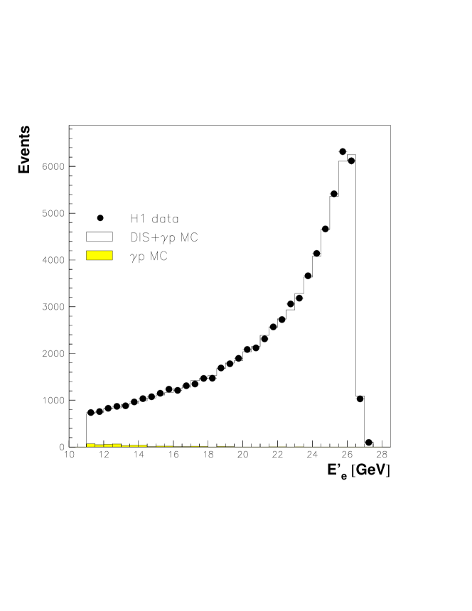
Fig. 23: The energy spectrum of the scattered electron from the 1993 H1 DIS data used in the extraction of $F_{2}$. The expectations from a Monte Carlo simulation are also shown, normalized to luminosity. The shaded histogram shows the estimation of the photoproduction background.

Another important requirement is the observation of approximate longitudinal energy-momentum conservation. The variable $\delta=(E-p_{Z})_{Observed}$ is calculated as

$$\delta=\sum_{i}E_{i}(1-cos\theta_{i})\;,$$ (90)

where the sum runs over clusters measured in the calorimeter and/or track momenta. The measured $\delta$ should equal $2E_{e}$ for perfect detector resolution and in the absence of energy leakage in the electron direction, which can arise from initial state QED radiation or from final state particle losses. A typical requirement is $\delta>35$ GeV. A $\delta$ spectrum as measured by ZEUS is shown in Fig. 24.

Fig. 24: The $\delta=E-P_{Z}$ distribution measured by the ZEUS experiment in the analysis of the 1994 DIS data. The solid points show the data which pass the cuts applied for the measurement of $F_{2}$ (except the $\delta$ cut). The open points show the $\delta$ distribution for photoproduction background events where the scattered electron has been measured in the luminosity electron detector. The DIS Monte Carlo simulation result is shown as the solid histogram while the dashed histogram shows the expectations from the photoproduction Monte Carlo simulation. The result of a fit to the data is shown as the dashed-dotted line. The contribution in the fit from photoproduction is shown separately as the dotted curve.

A minimum hadronic activity is also typically required in the analysis. This requirement is usually phrased in terms of the estimator of the inelasticity, $y$, calculated from the hadronic system. This estimator is calculated as follows (?):

$$y=\frac{\delta_{had}}{2E_{e}}\;,$$ (91)

where $\delta_{had}$ is the contribution to $\delta$ from the hadronic part of the event (i.e., excluding the scattered electron). The requirement on $y$ depends strongly on the type of kinematic reconstruction used.

Other selection criteria often employed are:

• A reconstructed event vertex within a defined range;

• Specific cuts to reject cosmic ray induced events or events initiated from muons in the proton beam halo;

• Timing cuts to reject events coming from upstream interactions of the proton or electron.

Backgrounds

There are several sources of background in the sample of DIS events chosen by the selection cuts listed above. These are:

• Photoproduction events where a calorimeter cluster has been falsely identified as the scattered electron (the scattered electron escapes down the beampipe). Photoproduction events are usually easily removed by requiring the observation of a high energy electron and a large $\delta$. However, these events can still pose a problem because of the very large photoproduction cross section (roughly a factor $100$ larger than the cross section for DIS with $Q^{2}>10$ GeV²). While electron identification is usually reliable, there are certain kinematical regions where it is difficult to distinguish photoproduction events from DIS events. The problem is most serious at large $y$, where the scattered electron and the fragmentation products of the scattered quark overlap spatially. Algorithms aiming for a high efficiency for selecting these events invariably find large background from photoproduction processes. Algorithms aiming for small backgrounds have low efficiencies in this kinematic region. Typical backgrounds range from 10 % in the larger $y$ bins, decreasing rapidly to a negligible level at $y\approx 0.5$.

• Scattering of beam particles with rest gas in the beam pipe. These types of interactions are both easily studied, using the unpaired electron and proton bunches, and also rather easily removed. They produce background below 1 %.

• QED Compton events ($ep\rightarrow ep\gamma$), where the final state electron and photon both end up in the main detector. They form part of the radiative corrections, but were not included in the event simulations used for the extraction of $F_{2}$. They must therefore be removed by algorithms specifically designed to select this final state.

The only significant background is from photoproduction. Great care must be taken in evaluating this background since it has a strong $y$ dependence, and could easily distort the measured $x$ dependence of the structure functions at small $x$. There are however several ways of estimating this background (see for example the $\delta$ spectrum in Fig. 24).

Cross section measurement

The cross section is determined in bins of $x$ and $Q^{2}$ (sometimes $y$ and $Q^{2}$) which are commensurate with the resolution. At small $Q^{2}$, bin sizes are chosen from a Monte Carlo study such that the fraction of events reconstructed in the same bin as that determined from the generated variables is larger than about $30$ %. This limits the size of the corrections which arise from unfolding the detector response. At larger $Q^{2}$, the bin sizes are generally set by requiring a minimum number of expected events in the bin. The cross section is determined from the number of events measured in a bin after corrections for background, inefficiencies, acceptances and resolution smearing, and the measured luminosity. The uncertainties in the luminosity measurements have steadily improved and are now at the $1.5$ % level.

Extraction of the structure function

The differential cross section for $e^{-}p$ NC scattering is given in terms of the of the structure functions $F_{2},F_{L}$ and $F_{3}$ as

$$\frac{d^{2}\sigma_{NC}}{dxdQ^{2}}=\frac{2\pi\alpha^{2}}{xQ^{4}}\left[Y_{+}F_{2}(x,Q^{2})-y^{2}F_{L}(x,Q^{2})+Y_{-}xF_{3}(x,Q^{2})\right]\;.$$ (92)

The variables $x$ and $Q^{2}$ are defined at the vertex of the Feynman graph where the gauge boson couples with the quark from the proton. The data are corrected for acceptance, resolution effects and radiative corrections using Monte Carlo methods before the differential cross sections are extracted.

The correction for $F_{L}$ is performed using the QCD prescription for $F_{L}$ given in Eq. (21). Target mass and higher twist effects are expected to be small and are ignored.

Note that $F_{2}=F_{2}^{EM}+F_{2}^{Weak}+F_{2}^{Int}$, where $F_{2}^{EM}$ represents the contribution from $\gamma$-exchange, $F_{2}^{Weak}$ the contribution from $Z^{0}$-exchange, and $F_{2}^{Int}$ the contribution from $\gamma-Z^{0}$ interference (see section 4.3.1). The value of $F_{2}^{EM}$ is often quoted separately. The contributions from $F_{2}^{Weak}\;{\rm and}\;F_{2}^{Int}$ become larger than a few percent above $Q^{2}=1000$ GeV², as does the contribution to the cross section from $F_{3}$. The effects of $W$ and $Z$ exchange are subtracted using standard parton density parameterizations. In the largest $Q^{2}$ bin measured, $Q^{2}=5000$ GeV², the $F_{3}$ correction reaches $22$ % for $e^{+}p$ scattering in the smallest $x$ bin measured, while the $Z^{0}$ contribution to $F_{2}$, including interference term, is $8$ %. It is expected that each of these contributions will eventually be individually measured at HERA.

4.3.4 HERA structure function results

Fig. 25: Comparison of the fixed target and HERA data at $Q^{2}=15$ GeV². The data span $3.5$ orders of magnitude in $x$ and match in a smooth way.

Fig. 26: The $F_{2}$ data from HERA and from fixed target experiments is plotted vs $x$ for different values of $Q^{2}$. The rise of $F_{2}$ towards smaller $x$ depends strongly on $Q^{2}$.

The HERA accelerator started delivering luminosity in 1992, and the experiments ZEUS and H1 have now each published several sets of proton structure function measurements (see Table 4). The first measurements showed the now well known rise of $F_{2}$ with decreasing $x$ at small $x$. These results were confirmed with the 1993 and 1994 data. The $(x,Q^{2})$ plane covered by the fixed target experiments, and by HERA, is shown in Fig. 4. As can be seen in this figure, the HERA results extended the $Q^{2}$ coverage at fixed $x$ by two orders of magnitude, and extended the $x$ range at fixed $Q^{2}$ by two orders of magnitude. The current data is of very high quality, as can be seen in the example shown in Fig. 25. Here, the HERA $F_{2}$ data is plotted vs $x$ for $Q^{2}=15$ GeV² and compared to the results from fixed target experiments. The HERA data matches on smoothly to the fixed target data. In this $Q^{2}$ range, the $F_{2}$ data now span nearly four orders of magnitude in $x$. The rise of $F_{2}$ with decreasing $x$ depends strongly on $Q^{2}$, as shown in Fig. 26. Increasing $Q^{2}$ implies that smaller transverse distance scales are probed. The number of quarks and antiquarks in the proton seen by the probe increases with decreasing momentum fraction, $x$, more rapidly as the distance scale is reduced.

Fig. 27: $F_{2}$ is plotted vs $x$ for the 1994 HERA data, and compared to results from fixed target experiments. $F_{2}$ shows a strong rise towards smaller $x$, with the strength of the rise increasing with $Q^{2}$. The curve represents the result of an NLO QCD fit performed by the ZEUS collaboration. It is able to reproduce the data down to $Q^{2}=1.5$ GeV².

The published HERA structure function measurements over the full kinematic range covered by the 1994 data are shown in Fig. 27. This figure includes the data from the different methods used to extract $F_{2}$ (nominal, shifted vertex and initial state radiation events). In some cases, several measurements from the same experiment are shown in overlapping kinematical ranges. The HERA data are in good agreement with each other, and with the fixed target data. The curves in the plots represent the results of a fit based on perturbative QCD (the NLO DGLAP evolution equation, described in section 2.3). It is found to reproduce the data well down to the smallest values of $Q^{2}$ in this plot. The success of the pQCD fit down to small $Q^{2}$ was quite surprising, and has generated a lot of interest in the small $Q^{2}$ region.

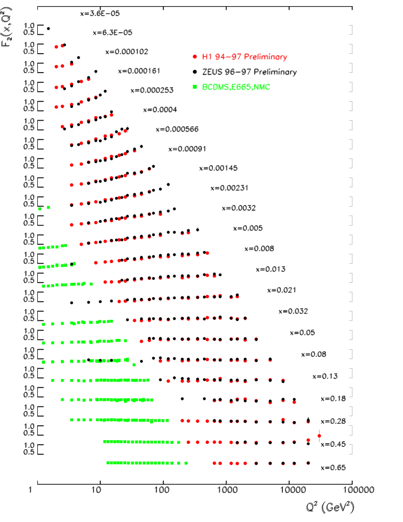
Fig. 28: $F_{2}$ is plotted vs $Q^{2}$ for fixed $x$ values for the preliminary 1994-97 HERA data, and compared to results from fixed target experiments. $F_{2}$ shows strong scaling violations, particularly at small $x$.

The preliminary 1994-97 $F_{2}$ results from HERA are shown versus $Q^{2}$, for fixed $x$, in Fig. 28. As can be seen in the figure, the more recent HERA data allow an extension of the $F_{2}$ measurements up to $Q^{2}=30,000$ GeV². Strong scaling violations are seen: $F_{2}$ increases with $Q^{2}$ at small $x$, while it decreases with increasing $Q^{2}$ at large $x$. This pattern of scaling violations is expected in QCD from gluon radiation from the quarks, and gluon splitting into quark-antiquark pairs. This radiation is made visible when the distance scale is reduced, and large $x$ quarks are resolved as a composite of quarks, antiquarks and gluons. The prediction of scaling violations is a success of QCD. The strong scaling violations at small $x$ point to the presence of a large gluon density; in fact, the measurement of the scaling violations leads to a determination of the gluon density in the proton, as explained in section 4.4.

Discussion of HERA Structure Function Results

The early measurements indicated that $F_{2}$ indeed rises quickly at small $x$, but not as quickly as predicted by the first BFKL approaches. The prediction of GRV was remarkably close to the HERA data down to much smaller $Q^{2}$ than initially expected. These developments had several effects:

1. The need for BFKL evolution could not be demonstrated, and it now seems unlikely that $F_{2}$ measurements will be able to separate BFKL from DGLAP evolution. Recent BFKL type calculations (?; ?) indicate a less steep rise of $F_{2}$ at small $x$, making it more difficult to separate from DGLAP evolution.

2. NLO DGLAP evolution, with appropriate parton distributions, is able to fit all structure function data down to values of $Q^{2}\approx 1$ GeV². There is no indication in $F_{2}$ of the onset of saturation in the kinematic range measured. The data are now precise enough that clear deviations are seen from the GRV prediction, but the accuracy of this prediction gave the first indication that the standard NLO DGLAP evolution could reproduce the bulk of the HERA structure function data.

3. The success of perturbative QCD down to small values of $Q^{2}$ has inspired new research into the predictions of the DGLAP equations. One such prediction goes by the name of double asymptotic scaling (?; ?). The DGLAP evolution equations are rewritten in terms of the variables

   $$\sigma = \sqrt{\ln\left(\frac{x_{0}}{x}\right)\ln\left(\frac{\alpha_{S}(Q_{0})}{\alpha_{S}(Q)}\right)}\;,$$ (93)

   $$\rho = \sqrt{\frac{\ln\left(\frac{x_{0}}{x}\right)}{\ln\left(\frac{\alpha_{S}(Q_{0})}{\alpha_{S}(Q)}\right)}}\;,$$ (94)

   where $Q_{0}$ and $x_{0}$ are parameters which must be determined experimentally. The measured values of $F_{2}$ are rescaled by functions $R_{F}(\sigma,\rho)$ and $R_{F}^{\prime}(\sigma,\rho)$ to remove the part of the leading sub-asymptotic behavior which can be calculated in a model independent way. The results for the H1 (?) $F_{2}$ measurements are shown in Fig. 29. Scaling is found to set in for $\rho\geq 2$ and $Q^{2}>5$ GeV². The measurement requires a value of $Q_{0}^{2}\approx 2.5$ GeV², while a value of $x_{0}=0.1$ was found to be a good choice. Although the physical meaning of these scaling variables is not clear, the results can be interpreted to indicate that the DGLAP formalism is valid down to small values of $Q^{2}$.

Fig. 29: The rescaled structure functions: top, $R_{F}F_{2}$ versus $\rho$; bottom, $log(R_{F}^{\prime}F_{2})$ versus $\sigma$ (see text). Only data with $Q^{2}\geq 5$ GeV² and $\rho>2$ are shown in the lower plot.

Deviation from NLO DGLAP evolution are now searched for at the edges of the available phase space. These include measurements down to $Q^{2}=0.11$ GeV² which probe the transition from non-perturbative to perturbative processes, measurements at large $y$, and measurements at very large $Q^{2}$. These are all discussed in the following sections.

Before we turn to these more detailed descriptions of the HERA data, we first review one outstanding inconsistency in the fixed target data, and see what HERA measurements can contribute to the debate.

4.3.5 Discrepancy in small-$x$ fixed target data

One outstanding discrepancy in the fixed target data involves the comparison of the $F_{2}$ data from the NMC (?), E665 (?) and CCFR (?) experiments at $x\approx 0.01$. The NMC and E665 data is for a muon beam on a proton target. The CCFR experiment used a neutrino beam on an iron target, where the data were corrected for nuclear effects as well as for the different propagator (photon versus $W,Z$) (?). At the smallest values of $x$ probed by these experiments, $x\approx 0.01$, the CCFR data lie about 15 % above the NMC data. This represents a much larger difference than can be accounted for by the normalization uncertainties quoted. At larger $x$, the discrepancy vanishes. Many theoretical ideas have been discussed for the discrepancy, such as effects related to the strange sea (?; ?), or charm threshold effects (?). As can be seen in Fig. 4, the HERA data has some overlap with the fixed target data in this region, and can be compared to the NMC, E665 and CCFR data. This is done in Fig. 30 for two different $x$ values. The HERA data tend to agree better with the CCFR data, despite experimental conditions which are more similar to those of the NMC and E665 experiments. These results need confirmation with more precise data from future measurements at HERA. Any theoretical explanation of the NMC, E665 and CCFR difference should also account for the HERA data.

Fig. 30: The HERA data compared to that from NMC, CCFR and E665 for $x\approx 0.01$. The $x$ value of the different data sets is given in the plot. Note that the expected change in $F_{2}$ from the differences in $x$ are much smaller than the NMC/CCFR difference. The NMC and E665 data are below the CCFR data by about 15 % in this $x$ range. The HERA data just begin to overlap the fixed target data, and are more compatible with the results from CCFR than those from NMC and E665.

4.3.6 $F_{2}$ at small $Q^{2}$

We now turn to a more detailed discussion of the small $Q^{2}$ structure function data at HERA. In photoproduction, it was found that the total cross section has a weak energy dependence similar to that found in hadron-hadron scattering. In contrast, a steep energy (or $x$) dependence was found in DIS. It is therefore very interesting to consider the transition region between these two different energy behaviors. As mentioned above, the ability of pQCD fits (in particular the success of the GRV parameterization, which predated these results) to reproduce the DIS data down to the lowest values of $Q^{2}$ initially available, $1.5$ GeV², inspired the ZEUS and H1 collaborations to make measurements at still smaller $Q^{2}$.

Several approaches have been used to access smaller $Q^{2}$, as described in section 3.5. These include using data sets with the interaction vertex shifted in the proton beam direction, thereby increasing the angular acceptance of the detectors at smaller electron scattering angles, and the addition of dedicated detectors at small angles to the electron beam direction such as the ZEUS beam pipe calorimeter (BPC). Events where the effective electron energy is reduced through tagged initial state radiation have also been employed, but these analyses tend to suffer from higher statistical and systematic uncertainties.

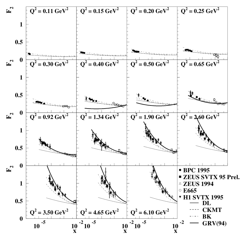
Fig. 31: The $F_{2}$ data at the lowest $Q^{2}$ values measured at HERA, compared to fixed target data from E665. $F_{2}$ is relatively flat at lower $Q^{2}$ values, and starts to show a rise at small $x$ around $Q^{2}\approx 1$ GeV². The $F_{2}$ data are compared to different parameterizations (see text for details).

The $F_{2}$ data at the smallest $Q^{2}$ values measured at HERA are shown in Fig. 31. $F_{2}$ is relatively flat at the smallest $Q^{2}$ values, and starts to show a rise at small $x$ for $Q^{2}\approx 1$ GeV². The data are compared to different parameterizations which we now describe.

1. The simplest of these parameterizations, from Donnachie and Landshoff (?), is labeled DL. It is an extension of a Regge based parameterization which was very successful in explaining inclusive cross section measurements in hadron-hadron and photoproduction data, as well as earlier fixed target DIS data. It clearly fails to reproduce the rise of $F_{2}$, and is systematically below the data at the smaller values of $Q^{2}$.

2. A more complicated Regge-type parameterization has been put forward by CKMT (?), which has a pomeron intercept changing with $Q^{2}$. The parameterization follows the rise of $F_{2}$, but lies below the data for $Q^{2}>1$ GeV².

3. The curve BK (?; ?) represents the predictions of a generalized vector dominance model (GVDM), matched to the GRV prediction at larger $Q^{2}$. It lies above the data at the smallest $Q^{2}$, and below the data for $Q^{2}>1$ GeV².

4. The curve labeled GRV is the prediction of Glück, Reya and Vogt. In their approach, the parton densities are parameterized at a very small $Q^{2}_{0}$ as consisting of valence quarks and gluons (?). The rise of the parton densities at small $x$ results from QCD radiative processes, which are calculated with the NLO DGLAP equation. The GRV parameterization lies below the data near its starting point of $Q_{0}^{2}=0.34$ GeV², and rises quickly with increasing $Q^{2}$ such that it lies above the data for $Q^{2}>1.3$ GeV².

Fig. 32: The values of $dF_{2}/d\ln Q^{2}$ for the HERA published data, compared to the prediction from the GRV parameterization (?). The fits to the HERA data have been performed by binning the data in $x$, and fitting a line $F_{2}=a+b\ln Q^{2}$. The central $x$ value of the bin is given on the horizontal axis. The central $\ln Q^{2}$ value of the bin is given at the top of the plot. The data slopes are also compared to the prediction from a Regge parameterization (see text) .

The behavior of the GRV curve indicates that the scaling violations predicted by this pQCD approach are much too strong at small $Q^{2}$. The scaling violations can be studied by plotting the data versus $Q^{2}$ in bins of fixed $x$. For this purpose, we have taken the published HERA data (ZEUS F2(BPC), F2(1994) and H1 F2(SVTX), F2(1994)) as of the fall of 1997. The statistical errors from the measurements were added in quadrature with the systematic errors, and a fit of the form

$$F_{2}=a+b\cdot\ln Q^{2}$$ (95)

was performed in bins of $x$. The slope $b$ is plotted in Fig. 32 and compared to the prediction from GRV. The slope in the data increases with decreasing $x$ down to $x\approx 10^{-4}$, at which point it turns over. The slope from GRV follows the data at larger $Q^{2}$, but overshoots the data for $Q^{2}$ smaller than about $4$ GeV², and shows no sign of decreasing at smaller $x,Q^{2}$. The underlying physics explanation for the turnover has yet to be determined. The slope $dF_{2}/d\ln Q^{2}$ is in leading order directly related to the gluon momentum density in the proton. The turnover at $(x,Q^{2})\approx(10^{-4},5~{}\rm{GeV}^{2})$ indicates that the gluons are starting to decrease in number as $(x,Q^{2})$ decrease. The reasons for this interesting observation are currently under investigation – one possibility is that this is a sign of shadowing corrections in DIS (?).

The behavior of Regge type parameterizations was studied by fitting a function of the form

$$F_{2}\propto\frac{M_{V}^{2}Q^{2}}{M_{V}^{2}+Q^{2}}W^{2\epsilon}\;,$$ (96)

where

$$\epsilon=\epsilon_{0}+\epsilon_{1}\cdot\ln(Q^{2}+Q^{2}_{0})\;,$$ (97)

to the ZEUS BPC data. The slope of $F_{2}$ from this type of parameterization is compared to the data in Fig. 32. The parameterization works well up to about $Q^{2}=1$ GeV². Beyond this value of $Q^{2}$, the predicted slope is much greater than seen in the data.

Fig. 33: The values of $dF_{2}/d\ln Q^{2}$ for fixed target data.

Note that the turnover of $dF_{2}/d\ln Q^{2}$ at small $(x,Q^{2})$ is not purely due to a $Q^{2}$ effect. This can be seen in Fig. 33, where $dF_{2}/d\ln Q^{2}$ for fixed target data is plotted in a similar way to HERA data. Similar values of $Q^{2}$ are reached, but at larger $x$. There is no indication for a turnover of the slopes.

The $dF_{2}/d\ln Q^{2}$ measurements can be reproduced by a general fit using the NLO DGLAP equations (?), albeit with rather curious parton densities. It is found from the fit that the gluon density vanishes at small-$x$ near $Q^{2}=1$ GeV². This is discussed in more detail in section 4.4.1.

Fig. 34: Variation of the exponent $\lambda$ from fits to the H1 data (?) of the form $F_{2}\sim x^{-\lambda}$ at fixed $Q^{2}$ values and $x<0.1$.

In Fig. 27 and 31, the slope of $F_{2}$ with decreasing $x$ is seen to increase with $Q^{2}$ in a smooth way. This behavior is quantified in Fig. 34, where the power $\lambda$, from a fit of the type $F_{2}\sim x^{-\lambda}$, is shown to decrease smoothly with $Q^{2}$. It reaches values near the photoproduction result ($0.16$) near $Q^{2}=1$ GeV². If we associate the steep rise of the structure function with the presence of perturbative QCD processes, then this result also indicates that pQCD processes become important around $Q^{2}=1$ GeV².

These results lead to the conclusion that non-perturbative effects dominate for $Q^{2}<1$ GeV², whereas pQCD processes dominate the cross section above $Q^{2}\approx 5$ GeV². The HERA data span this transition, and may therefore yield insight into non-perturbative QCD processes.

4.3.7 $F_{L}$

The measurement of $F_{L}$ is very important to test the reliability of pQCD calculations, since its value is predicted from the gluon density and $F_{2}$ (see Eq. (21)). In addition, the uncertainty in $F_{L}$ limits the accuracy with which $F_{2}$ can be determined. As can be seen in Eq. (72), the contribution to the differential cross section from $F_{L}$ is suppressed by $y^{2}/Y_{+}$ relative to $F_{2}$. Given the bound $F_{L}\leq F_{2}$, the $F_{L}$ contribution will be small at small $y$. However, the particularly interesting small-$x$ region corresponds to large $y$, where the $F_{L}$ contribution cannot be ignored. The usual procedure adopted experimentally for the extraction of $F_{2}$ is to use, in the region of moderate $x$, the parameterization for the ratio $R\approx F_{L}/(F_{2}-F_{L})$ based on the dedicated SLAC measurements (?) and, at small $x$, the QCD expectations based on existing parton distributions.

The experimental determination of $F_{L}$ requires the measurement of the differential cross section at different center-of-mass energies. This allows a different value of $y$ for the same $(x,Q^{2})$, and therefore a separation of $F_{2}$ and $F_{L}$. This is unfortunately a very difficult measurement, as it requires the difference of cross sections. The measurement at HERA would require the reduction of the proton and/or electron beam energy, and will likely be performed before HERA running is completed.

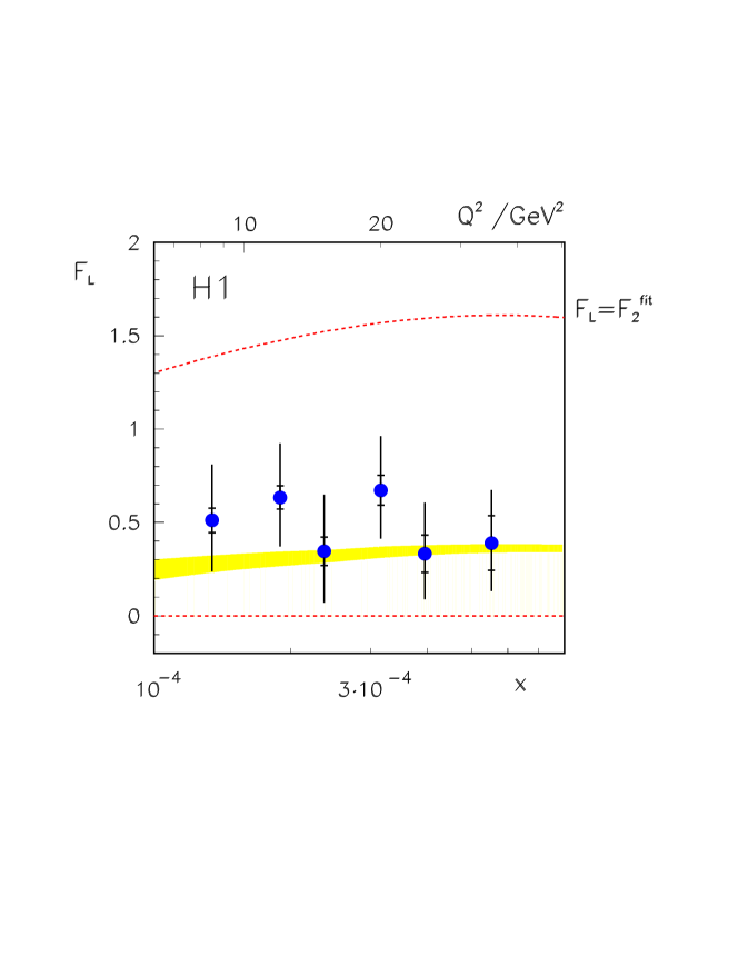
Fig. 35: $F_{L}$ as a function of $x$ (and $Q^{2}$) as determined by the ?. The shaded band corresponds to NLO QCD expectations using the parton densities extracted by H1.

The H1 Collaboration (?) has estimated $F_{L}$ by assuming that the DGLAP evolution equations are capable of describing the evolution of $F_{2}$. In this method, the cross section, and $F_{2}$, are initially extracted at small $y$ where the contribution from $F_{L}$ is small. The NLO DGLAP equations are then used to extrapolate $F_{2}$ to large $y$, where the cross section contribution from $F_{2}$ is compared to the measured cross section. The difference in cross sections is attributed to $F_{L}$. The results of this procedure are shown in Fig. 35. Within errors, there is good agreement between the extracted value of $F_{L}$ and the expected value from pQCD. The expectations for $F_{L}$ obtained from a QCD fit and assuming that $F_{L}=F_{2}$ is also shown. This value of $F_{L}$ is clearly ruled out.

4.3.8 $F_{2}^{c\bar{c}}$

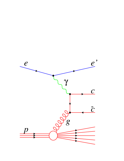
Fig. 36: The leading order diagram for charm production via photon-gluon fusion.

The measurement of $F_{2}$ is based on the inclusive cross section for $ep$ scattering. It is also possible to define the contributions to $F_{2}$ which result in particular final states. This is useful in cases where the relevant cross section can be calculated theoretically. One such example is for charm production in DIS. The reaction $ep\rightarrow ecX$, where $c$ represents a charm quark or anti-quark, is expected theoretically to proceed primarily via photon-gluon fusion, $\gamma g\rightarrow c\bar{c}$. This process is shown in Fig. 36 for the leading order diagram. Calculations for this process exist theoretically to NLO (?; ?; ?). The cross section depends directly on the gluon density in the proton. The gluon density from the inclusive analysis can be used in the calculation, and the results compared to the measured charm cross sections. This gives a powerful cross check on the pQCD calculations.

There are other processes beside photon-gluon fusion which can produce charm in DIS: diffractive heavy flavor production (?), scattering off charmed sea quarks (?), charmed hadron production from bottom quarks (?), charm production in fragmentation (?; ?; ?), and intrinsic charm in the proton (?). These processes have either been measured to have small cross sections relative to the photon-gluon fusion mechanism, or are not expected to contribute in the relevant kinematic regions.

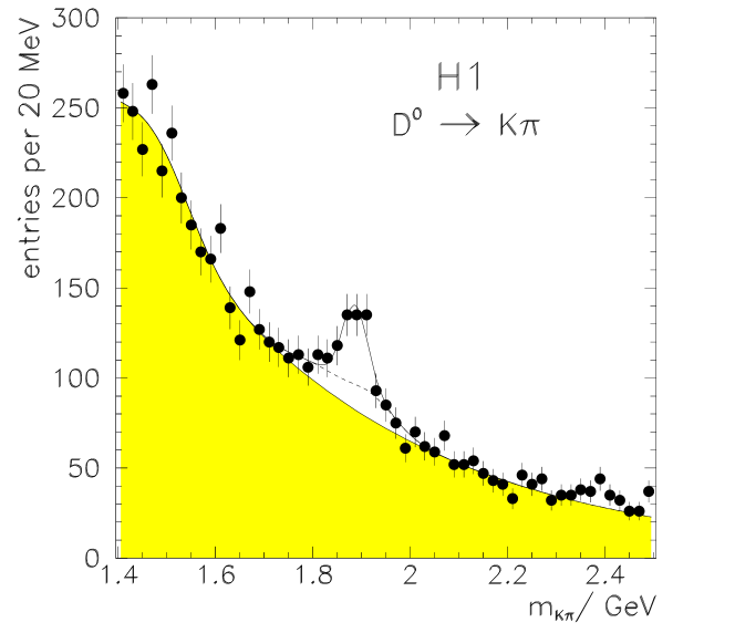
Fig. 37: The two particle invariant mass spectrum obtained when assigning the $K^{\pm}$ mass to one of the particles and the $\pi^{\pm}$ mass to the other, as measured by the ?.

Fig. 38: a) The $\Delta M=M(K\pi\pi_{s})-M(K\pi)$ distribution for $M(K\pi)$ in the $D^{0}$ signal region, where $\pi_{s}$ denotes the softest pion. b) The $M(K\pi)$ distribution for events in the $\Delta M$ signal region. The results are from the ?.

Results on charm production in DIS have been presented by H1 (?) and ZEUS (?; ?). Charm production is tagged by reconstructing the $D^{0}$ (H1) or the $D^{*}$ (H1 and ZEUS) mesons and their charge conjugates. The signal for $D^{0}\rightarrow K\pi$ as seen in the H1 detector is presented in Fig. 37. The $D^{*}$ decays are identified by the decay chain $D^{*}\rightarrow D^{0}\pi\rightarrow K\pi\pi$, taking advantage of the tight kinematic constraint imposed by the small mass difference $\Delta M=m_{D^{*}}-m_{D^{0}}=145.5\pm 0.15$ MeV. As an example the signal observed in the $\Delta M$ distribution by ZEUS is shown in Fig. 38.

As described above, the dominant mechanism for charm production in DIS at HERA energies is expected to be the photon-gluon fusion process. Indeed, the AROMA (?) Monte Carlo simulation program based on this process is found to reproduce properly the shapes of the transverse momentum and pseudorapidity spectra for the $D$ mesons, as well as the overall $W$ and $Q^{2}$ dependences. An upper limit of $5$ % on a possible contribution of the charm sea has been estimated by H1.

The charm production cross section has been measured by the H1 collaboration in the kinematic range $10\leq Q^{2}\leq 100$ GeV² and $0.01<y<0.7$. The measurements are performed within experimentally accessible regions (various cuts are applied on the tracks from the charmed hadrons, leading to $p_{T}$ and $\eta$ restrictions) and are then extrapolated to the full phase space using the AROMA Monte Carlo simulation. The result is found to be somewhat larger than predicted. This is true for all gluon density parameterizations used, including the gluon density measured by H1 from the scaling violations of $F_{2}$. The latter gluon density gives the best agreement with the measurement. For $m_{c}=1.5$ GeV, the prediction using the H1 gluon density is $13.6$ nb, while the measured cross section is $17.1\pm 2.3$ nb.

The ZEUS experiment finds, for the same kinematic region, a measured cross section of $12.5\pm 3.9$ nb, in reasonable agreement with the H1 measurement. They find for the NLO prediction, with $m_{c}=1.5$ GeV and the GRV NLO gluon density (?), a value of $11.1$ nb, and conclude that this is in good agreement with the data. The NLO predictions are also able to reproduce the shapes of the $p_{T},\;W$ and $Q^{2}$ distributions, and is consistent with the $\eta$ distribution measured in the data. ZEUS then extrapolates into the unmeasured region using NLO calculations (?; ?).

$F_{2}^{c\bar{c}}$ is calculated from the measured charm cross section as follows:

1. The cross section for $c\bar{c}$ production is calculated from the $D^{*}$ cross section (extrapolated to the full phase space), using

   $$\sigma(ep\rightarrow ec\bar{c}X)=\frac{1}{2}\frac{\sigma(ep\rightarrow eD^{*}X)}{P(c\rightarrow D^{*})}\;,$$ (98)

   where $P(c\rightarrow D^{*})$ is the probability that a charm quark will produce a $D^{*}$ meson (about 25 %).

2. The measurements are made at small $Q^{2}$, such that $F_{3}$ can be neglected. Also, the possible contribution from $F_{L}$ has been estimated to be small and is ignored. $F_{2}^{c\bar{c}}$ is then extracted using

   $$\frac{d^{2}\sigma(ep\rightarrow ec\bar{c}X)}{dxdQ^{2}}=\frac{2\pi\alpha^{2}}{xQ^{4}}\left[Y_{+}F_{2}^{c\bar{c}}(x,Q^{2})\right]\;.$$ (99)

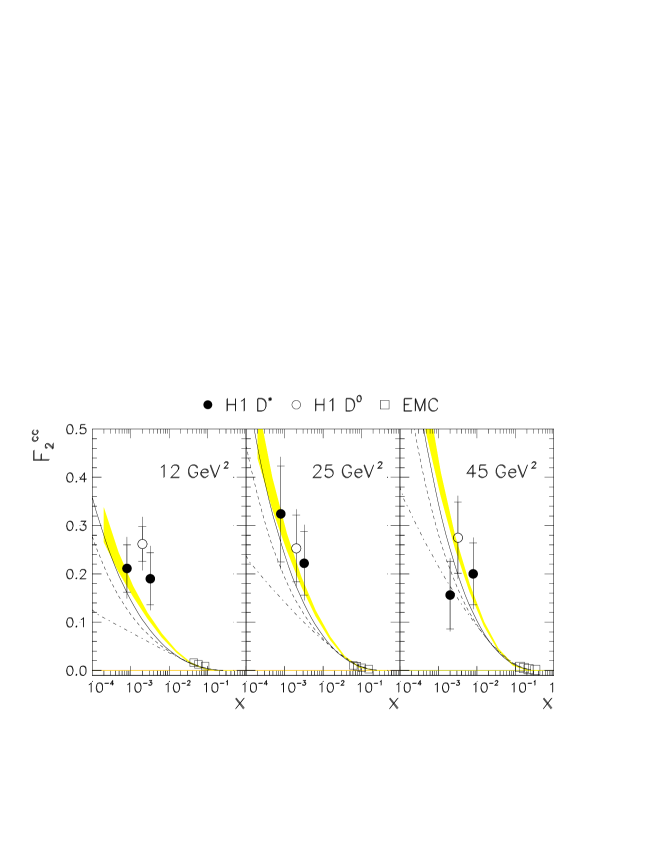
Fig. 39: $F_{2}^{c\bar{c}}$ as measured by the H1 experiment (?). The curves correspond to different parton parameterizations: GRV-H0 (full line), MRSH (dashed line), and MRSD0’ (dashed-dotted line). The shaded area is the expectation based on the H1 NLO QCD fit. The EMC data are also shown as open boxes (?).

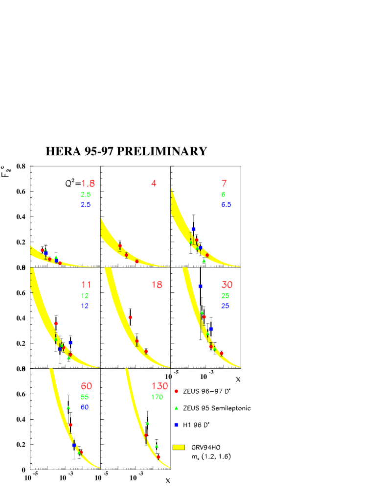
Fig. 40: $F_{2}^{c\bar{c}}$ as measured by the ZEUS experiment from the 1995-97 data sets (?). The $Q^{2}$ values in the figure are in GeV². The shaded area is the expectation using the GRV94(HO) parton density set, allowing for a range of charm quark masses between $1.2<m_{c}<1.6$ GeV.

The first results on $F_{2}^{c\bar{c}}$ as measured by the H1 collaboration are shown in Fig. 39, and compared with the EMC (?) measurements. The data reveal a steep rise of $F_{2}^{c\bar{c}}$ as $x$ decreases from $x=0.1$ to $x=10^{-3}$. Averaged over the kinematical range of H1, a ratio $<F_{2}^{c\bar{c}}/F_{2}>=0.237\pm 0.021^{+0.043}_{-0.039}$ is obtained, one order of magnitude larger than at large $x$.

The latest preliminary results from HERA (?; ?) on $F_{2}^{c\bar{c}}$, based on data up to 1997, is shown in Fig. 40. The measurements are seen to be in good agreement. They are compared to the predictions from NLO calculations (?; ?) using as input the gluon density parameterization from GRV. The agreement is good, indicating that the pQCD description of the data is self-consistent.

The data available so far are in good agreement with expectations from NLO pQCD calculations. However, the statistical errors are still quite large, and the data span a rather limited kinematic range. A large increase in statistics is forthcoming, and it is expected that the $F_{2}^{c\bar{c}}$ measurements will eventually reach a precision level similar to that for the inclusive $F_{2}$ measurements presented in this review. The evolution of $F_{2}^{c\bar{c}}(x,Q^{2})$ is a matter of some theoretical debate. Some authors (?; ?) start with zero charm content in the proton below some scale $Q^{2}_{0}\sim m_{c}^{2}$, and then evolve charm as a massless quark above this threshold. A second approach is to generate charm exclusively via photon-gluon fusion taking into account the charm quark mass (?). A third approach consists of having a variable flavor number scheme (?). More precise data will allow much more stringent tests of the pQCD calculations, and should allow to discriminate between these, and possibly other, approaches to calculating the charm content of the proton.

4.4 The gluon density in the proton

The behavior of many of the cross sections measurable at HERA is driven by the gluon density in the proton. This results from the fact that, due to experimental cuts, most cross sections are measured in the large-$W$, or small-$x$, domain. Small-$x$ quarks are therefore involved in the reaction. The distribution of the small-$x$ quarks is determined principally by the gluon density in the proton via $g\rightarrow q\bar{q}$ splitting. The cross sections for diverse reactions such as open charm production, jet production, vector meson production, as well as inclusive cross sections, can be used to measure the gluon density in the proton. The consistency of the gluon densities extracted via these different methods provides a measure of how well the pQCD expansions can currently be used for calculational purposes. The measurement of the gluon density therefore serves a two-fold purpose: it is necessary to know the gluon density to calculate cross sections for current as well as future experiments; and, assuming the validity of QCD, the consistency of different methods of measuring the gluon density is a measure of calculational ability. Discrepancies in the gluon densities beyond theoretical and experimental uncertainties would be a sign that QCD does not provide a complete description of the strong interactions.

There are very different levels of theoretical sophistication for the various methods proposed for the extraction of the gluon density. The extraction based on the total DIS cross section (fits to $F_{2}$) has a long experimental as well as theoretical history, and is the most advanced. Many NLO evolution programs exist which give consistent results at the fraction of a percent level (?). Most other methods are based on LO QCD calculations, and therefore suffer from large normalization uncertainties (factors of two are possible). Generally, the $x$- or $W$-dependence of the cross sections are more firmly predicted, such that the shape of the gluon density is then constrained. In the following sections, we review in some detail the extraction of the gluon density from the inclusive cross section measurement, and then briefly describe other proposed methods.

4.4.1 Gluon density extraction from $F_{2}$

The DGLAP evolution equations relate the change with $Q^{2}$ of the quark densities in the proton, $q(x,Q^{2})$, or equivalently the structure function $F_{2}(x,Q^{2})$, to the density of gluons, $g(x,Q^{2})$. For example (?),

$$\frac{dF_{2}(x,Q^{2})}{d\ln Q^{2}} = \frac{\alpha_{s}(Q^{2})}{2\pi}\left[\int_{x}^{1}\frac{dz}{z}\frac{x}{z}P_{qq}\left(\frac{x}{z}\right)F_{2}(z,Q^{2})\right.$$ (100)

$$\mbox{ }\left.+2\sum_{q}e_{q}^{2}\int_{x}^{1}\frac{dz}{z}\frac{x}{z}P_{qg}\left(\frac{x}{z}\right)zg(z,Q^{2})\right]\;,$$

where the sum runs over quark flavors, and $e_{q}$ is the quark charge. $P_{qq}$ and $P_{qg}$ are the splitting functions to quarks of the quark and gluon, respectively. To leading order they are given by (see, e.g., (?; ?; ?))

$$P_{qq}(z) = C_{F}\left[\frac{1+z^{2}}{1-z}\right]\;,$$ (101)

$$P_{qg}(z) = D_{F}[z^{2}+(1-z)^{2}]\;,$$ (102)

where the multiplicative constants are color factors. As a result, the $Q^{2}$ dependence of the parton densities may be calculated provided their $x$ dependence is known from data at some lower $Q^{2}$. A common approach is to parameterize at fixed $Q^{2}=Q^{2}_{0}$ the $x$ dependence of the parton densities by

$$x\cdot{\rm density}(x,Q^{2}_{0})=Ax^{\delta}(1-x)^{\eta}\cdot{\rm polynomial}(\sqrt{x})\;,$$ (103)

with a distinct set of parameters for each type of parton. The parton densities are then determined by applying the evolution equations to perform a global fit of all the parameters to deep inelastic scattering data. This approach has been used by the ZEUS (?; ?) and H1 (?; ?) collaborations using their 1993, 1994 and 1995 $F_{2}$ measurements.

H1 DGLAP fits

The H1 collaboration (?) performed NLO DGLAP fits to $F_{2}$ data by defining parton densities in the $\overline{MS}$ renormalization scheme. Three light flavors of quarks were taken into account. The charm quark contribution was generated dynamically using the photon-gluon fusion prescription given in (?; ?), with scale $\sqrt{Q^{2}+4m_{c}^{2}}$. The charm quark mass was set to $m_{c}=1.5$ GeV. Beauty quark contributions are expected to be small and were neglected.

The specific functional forms used by H1 were

$$\begin{array}[]{rcl}xg(x,Q^{2}_{0})&=&A_{g}x^{\delta_{g}}(1-x)^{\eta_{g}}\;,\\ xu_{v}(x,Q^{2}_{0})&=&A_{u}x^{\delta_{u}}(1-x)^{\eta_{u}}(1+B_{u}x+C_{u}\sqrt{x})\;,\\ xd_{v}(x,Q^{2}_{0})&=&A_{d}x^{\delta_{d}}(1-x)^{\eta_{d}}(1+B_{v}x+C_{d}\sqrt{x})\;,\\ xS(x,Q^{2}_{0})&=&A_{S}x^{\delta_{S}}(1-x)^{\eta_{S}}(1+B_{S}x+C_{S}\sqrt{x})\;,\end{array}$$ (104)

where the glue, valence $u$ and $d$ and sea, $S\equiv\bar{u}+\bar{d}$, quarks have distinct parameters. The quark and antiquark components of the sea are assumed equal, and $\bar{u}$ is set equal to $\bar{d}$. The strange quark density is set to be $S/4$ (?). The normalizations of the valence quark densities were fixed by the counting rules

$$\begin{array}[]{rcl}\int_{0}^{1}u_{v}(x)dx&=&2\;,\\ \int_{0}^{1}d_{v}(x)dx&=&1\;.\end{array}$$ (105)

The normalization of the gluon density, $A_{g}$, was obtained via the momentum sum rule. The further constraint $\delta_{u}=\delta_{d}$ was imposed.

The fits were performed with $Q_{0}^{2}=5$ GeV² and $\Lambda_{4}^{\overline{MS}}=263$ MeV. In addition to the H1 data, the proton and deuteron results from BCDMS (?) and NMC (?) were used to constrain the parton densities at large $x$. Data in the range $Q^{2}>5$ GeV² were fit, except for data with $x>0.5$ and $Q^{2}<15$ GeV².

Fig. 41: Compilation of measurements of $F_{2}$ as a function of $Q^{2}$ for selected values of $x$ as denoted on the figure. The numbers in parentheses are the scaling factors by which the value of $F_{2}$ has been multiplied in the plot. The overlayed curves are the result of an NLO QCD fit performed by the H1 experiment to H1, NMC and BCDMS data.

The fits to the $F_{2}$ data are shown in Fig. 41 compared to HERA and fixed target data. Data not used in the fitting procedure are also shown. As can be seen in this figure, the fits reproduce the data quite well. The values of the parameters extracted in the fits are given in Table 5. The value of $\delta$ is negative for both the gluon and sea quark density, indicating that these densities rise with decreasing $x$.

Table 5: The values of the parameters for the parton density parameterizations as extracted by H1 (?) and ZEUS (?) from NLO DGLAP fits to structure function data. The parameters are given in the H1 case for $Q_{0}^{2}=5$ GeV², and in the ZEUS case for $Q_{0}^{2}=7$ GeV². The form of the parameterizations are given in the text.

	H1 fit result					ZEUS fit result
	$A$	$\delta$	$\eta$	$B$	$C$	$A$	$\delta$	$\eta$	$B$	$C$
$xg$	$2.24$	$-0.20$	$8.52$			$1.77$	$-0.225$	$9.07$	$3.00$
$xu_{v}$	$2.84$	$0.55$	$4.19$	$4.42$	$-1.40$
$xd_{v}$	$1.05$	$0.55$	$6.44$	$-1.16$	$3.87$
$x(\bar{u}+\bar{d})$	$0.27$	$-0.19$	$1.66$	$0.16$	$-1.00$
$x(u+\bar{u}-d-\bar{d})$						$6.07$	$1.27$	$3.68$
$2x(\bar{u}+\bar{d}+\bar{s})$						$0.52$	$-0.24$	$8.60$	$3.27$	$0.29$

ZEUS DGLAP fits

The most recent results from the ZEUS collaboration are presented in (?). The fits were performed on the ZEUS 1994 F2 data as well as the 1995 shifted vertex data presented in  (?). NMC (?) and BCDMS (?; ?) results are used to constrain the large-$x$ parton densities. ZEUS defined the parton densities at an input scale $Q^{2}_{0}=7$ GeV², and fit data down to $Q^{2}=1$ GeV². The gluon, sea quark $S=2(\bar{u}+\bar{d}+\bar{s})$, and difference of up and down quarks in the proton $\Delta$ were parameterized as

$$\begin{array}[]{rcl}xg(x,Q^{2}_{0})&=&A_{g}x^{\delta_{g}}(1-x)^{\eta_{g}}(1+B_{g}x)\;,\\ xS(x,Q^{2}_{0})&=&A_{S}x^{\delta_{S}}(1-x)^{\eta_{S}}(1+B_{S}x+C_{S}\sqrt{x})\;,\\ x\Delta_{ud}(x,Q^{2}_{0})&=&A_{\Delta}x^{\delta_{\Delta}}(1-x)^{\eta_{\Delta}}\;.\end{array}$$ (106)

The input valence distribution $xu_{v}=x(u-\bar{u})$ and $xd_{v}=x(d-\bar{d})$ were taken from the parton distribution set MRS(R2) (?). The strange quark density was assumed to be $20$ % of the sea at $Q^{2}=1$ GeV². The gluon density normalization was fixed using the momentum sum rule. The input value of the strong coupling constant was set to $\alpha_{s}(M_{Z}^{2})=0.118$.

The parton densities are defined in the $\overline{MS}$ scheme, and were evolved using the NLO DGLAP equation with three light flavors. The charm contribution was calculated in NLO using the calculations of Riemersma et al. (?) with the charm quark mass set to $m_{c}=1.5$ GeV. The values of the fit parameters are given in Table 5.

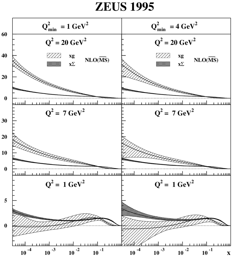
Fig. 42: The quark singlet momentum distribution, $x\Sigma$ (shaded), and the gluon distribution, $xg$ (hatched), as functions of $x$ from the ZEUS NLO QCD fits. The three left-hand plots show the results including $F_{2}$ data with $Q^{2}>1$ GeV²; the three right-hand plots show the corresponding results for data with $Q^{2}>4$ GeV².

As mentioned previously, the ZEUS DGLAP fit is able to reproduce the turnover in the scaling violations plot. However, this is only possible with a rather non-intuitive result for the parton densities. The gluon density is seen to dominate at small-$x$ for moderate $Q^{2}$, but decreases sharply as $Q^{2}$ approaches $1$ GeV², at which point it is smaller than the sea quark density, and essentially valence-like. The gluon density found by ZEUS is compared to the sum of the quark distributions, $x\Sigma$, in Fig. 42. It is at this point not clear whether the parton densities at these small values of $Q^{2}$ are meaningful (i.e., could be used to predict a cross section for a different process), or result from non-perturbative contributions to the cross section. It is not possible to determine from the existing data where the DGLAP fit is no longer valid. The flexibility in the parton density parameterizations is such that the fits find solutions. Other criteria must be found to determine whether the results are sensible.

Discussion

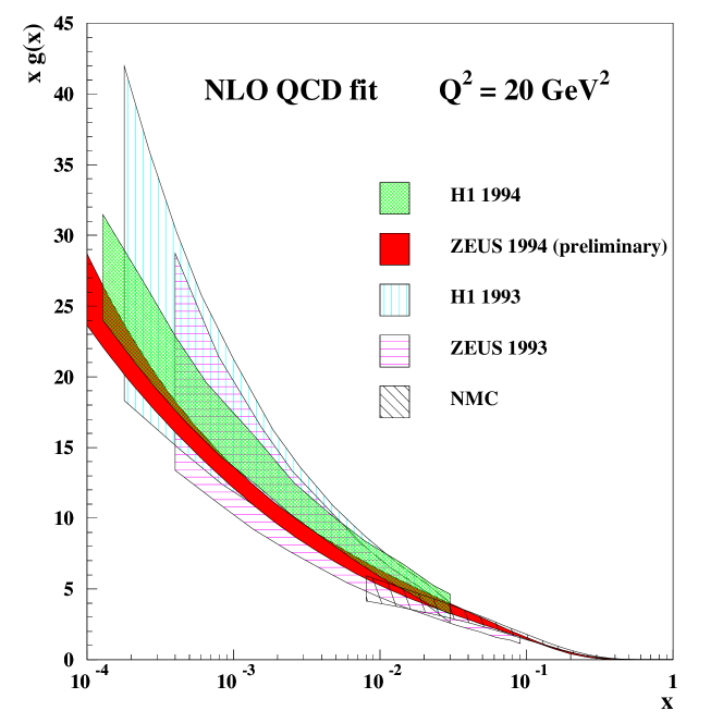
Fig. 43: The gluon distribution in the proton as determined from NLO QCD fits to the $F_{2}$ data. The results from the 1993 data are compared to those from the 1994 data.

The results for the extracted gluon density for ZEUS and H1 are compared to those from NMC in Fig. 43. The NLO gluon density is now known at the $10$ % level from these fits. This is currently the most precise determination of the gluon density in the proton.

There are several points to be made regarding this method of extracting the gluon density:

• The DGLAP fits are performed on the extracted $F_{2}$, which were determined from the measured differential cross section. In the process of extracting $F_{2}$, the contribution from $F_{L}$ is calculated assuming some gluon density and subtracted. Different parameterizations for the gluon density are used to test the sensitivity of $F_{2}$ to this choice. The resulting change in the extracted gluon density was found to be small.

• The HERA data alone are not sufficient to constrain the gluon density. The normalization, $A_{g}$, and large-$x$ behavior, $\eta_{g}$, are primarily determined by the fixed target data. Relative normalization differences in different experimental data sets and correlated errors must be handled carefully.

• The extracted gluon density depends on $\alpha_{s}$, which also evolves with $Q^{2}$. The value of $\alpha_{s}$ is taken from other experiments.

• The validity of the DGLAP evolution equation across a transition from a flat parton density (at some small value of $Q^{2}$) to a steep parton density has been called into question (?). This could limit the range in $Q^{2}$ over which the fits can be performed to the $Q^{2}$ region where the parton densities have been shown to be steep.

Despite these caveats, it should be stressed that the gluon density is now known rather precisely at small-$x$. Given the factorization theorem described in section 2.3, this allows precise predictions for cross sections of many processes at HERA, and for other experiments utilizing protons.

4.4.2 Other gluon density extraction methods

Heavy quark production

The production of heavy quarks, both in photoproduction and DIS, is sensitive to the gluon density inside the proton. At HERA, this principally means charm quark production. We can distinguish between open charm production, where hadrons with net charm quantum numbers are produced, and the production of $c\overline{c}$ bound states ($J/\psi$ and excited states.) The latter are described in section 7, while open charm production in DIS has been described above in section 4.3.8. It is believed that photoproduction reactions can also be used for this purpose. In this case, the sizeable charm mass as well as the transverse energy of the charm particles set the scale at which the gluon density is probed.

Full NLO calculations for charm photoproduction cross sections are available. They are distinguished in the method in which the charm mass is handled. In the so-called ‘massive-charm’ scheme, the mass of the charm quark acts as a cutoff in the perturbative calculation (?; ?). In the ‘massless-charm’ scheme, the charm is treated as one of the active flavors in the proton and photon (?; ?; ?; ?). A significant difference between the two schemes is that in the massive scheme the cross section is dominated by photon-gluon fusion, while in the massless scheme the contribution from resolved photons is of comparable size.

Fig. 44: The differential cross section $d\sigma/dp_{\perp}^{D^{*}}$ for $D^{*}$ photoproduction in the kinematic range $Q^{2}<1$ GeV², $130<W<280$ GeV and $-1.5<\eta^{D^{*}}<1.0$ from the ?. The data are compared to various calculations as described in the text.

Fig. 45: The differential cross section $d\sigma/d\eta^{D^{*}}$ for $D^{*}$ photoproduction in the kinematic range $Q^{2}<1$ GeV², $130<W<280$ GeV and different minimum $p_{\perp}^{D^{*}}$. The curves represent the NLO calculations under the same conditions as for figure 44.

Recent data (?) for $d\sigma_{ep\rightarrow D^{*}X}/dp_{T},\;d\sigma_{ep\rightarrow D^{*}X}/d\eta$. and $d\sigma_{ep\rightarrow D^{*}X}/dW$, measured by the ZEUS collaboration, are shown in Figs. 44,45 and compared to different theoretical calculations. Both calculations using standard settings of the charm mass and renormalization scales are low relative to the data, although the absolute magnitude of the cross section calculated in the massless approach agree better with the data. The deficit of the calculations appears to reside primarily at large $\eta$. There are indications that this may be due to an intrinsic charm content in the photon, which has very weak experimental constraints.

It is clear that a better control of the theoretical and experimental issues must be obtained before this method can be used to extract the gluon density in the proton. The corrections with respect to leading order are substantial, as is the remaining scale uncertainty in the NLO calculations. There is also sensitivity to the structure of the photon, particularly in the massless scheme, and theoretical calculations of the cross section suffer from a number of uncertainties, such as the appropriate value of the charm mass and the choice of scale for the process.

Vector meson production

The sensitivity of exclusive vector meson production to the gluon density in the proton is described in detail in section 7. The strength of this method is that the cross sections depend, in pQCD, on the square of the gluon density, and are therefore very sensitive to the $x$ dependence of the gluon density. However, full calculations are not available in NLO and therefore normalization uncertainties are large. The scale at which the gluon density should be evaluated is not clear, at least at small $Q^{2}$, and questions have been raised relating to the correlation function between the gluons involved in the scattering. If these theoretical issues can be successfully addressed, then elastic vector meson production may indeed become the method of choice for the gluon density measurement.

Fig. 46: Inelastic $J/\psi$ production via photon-gluon fusion. This is one of several possible diagrams where a $J/\psi$ can be produced in an inelastic reaction.

Inelastic $J/\psi$ production has also been proposed as a means for extracting the gluon density. In this process, as with open charm production, the incoming photon couples to a single gluon via a virtual $c\bar{c}$ pair (Fig. 46). Full NLO pQCD calculations exist for this process (?; ?) in the framework of the color singlet model (?), in which $J/\psi$ production proceeds via photon-gluon fusion followed by the emission of a hard gluon in the final state. The color-octet model (?) includes, additionally, the production of the $J/\psi$ in a color-octet state, which then becomes a color-singlet via the emission of a soft gluon. This model, developed to explain hadroproduction data (?; ?), attempts to include non-perturbative effects and requires parameter tuning. Other mechanisms for inelastic $J/\psi$ production are diffractive production with proton dissociation, and production via resolved photons. The latter two can be effectively isolated experimentally by cutting on $z$, the fraction of the photon energy, evaluated in the proton rest frame, carried by the $J/\psi$. Resolved photon production is expected to populate the low $z$ region, while diffractive production peaks at $z=1$. Color-octet contributions are also expected to populate the large $z$ region.

Fig. 47: Inelastic $J/\psi$ production cross section as a function of $W$ from ZEUS (?) and H1 (?). The lines correspond to the NLO pQCD prediction from (?; ?) for the three different parton density sets shown in the plot.

Fig. 48: The differential cross section versus $z$ for inelastic $J/\psi$ production at HERA in the kinematic range $50<W<180$ GeV and $p_{T}^{2}>1$ GeV². The solid line is the prediction from the color-singlet model using as input the GRV parton densities. The dashed line represents the sum of the color-singlet and color-octet contributions.

The experimentally measured cross sections (?; ?) are shown as a function of $W$ in Fig. 47, where they are compared to NLO calculations (?) with different gluon density parameterizations. There is good agreement between the data and the NLO calculations. It is also clear from the figure that it will be very difficult to use this process to distinguish different gluon densities. This results in large part from the experimental cuts needed to select the sample - the requirement of a minimum $p_{T}$ of the $J/\psi$ limits the $x$ range which can be probed at HERA. The HERA data are plotted as a function of $z$ in Fig. 48, and clearly show a preference for a pure color singlet contribution. However, it should be mentioned that the color-octet contributions are non-perturbative, and that considerable theoretical work is ongoing to refine the predictions.

Jet production

The cross section for the production of jets in photoproduction and DIS also depends on the gluon density via the photon-gluon fusion mechanism. It is important to separate the contribution to the cross section from photon-gluon fusion from that due to QCD-Compton scattering. These processes are shown in LO in Fig. 10. The fractional momentum carried by the parton entering in the hard interaction is given by

$$\xi=x\frac{Q^{2}+\hat{s}}{Q^{2}}\;,$$ (107)

where $x$ is the usual Bjorken scaling variable and $\hat{s}$ is the invariant mass of the two jets. The density of partons can be extracted from the measured rate of dijet events and the calculable hard scattering reaction cross section.

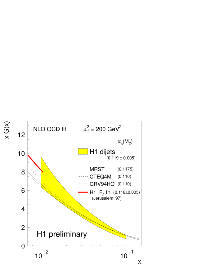
Fig. 49: The gluon momentum density in NLO measured from dijet rates in DIS by the ?. The gluon density is probed at an average $\mu^{2}$ of $200$ GeV² and is for a value of $\alpha_{S}(M_{Z}^{2})=0.119\pm 0.005$. The result is compared to the gluon density extracted by H1 from a fit to $F_{2}$, and to other parton density parameterizations.

The H1 collaboration has extracted a LO value for the gluon density by studying dijet production in DIS (?). A NLO extraction of the gluon density from this method is quite desirable. The latter has been attempted by the H1 collaboration (?). The results of this analysis are shown in Fig. 49. The data are consistent with a steep rise of the gluon density found from the analysis of $F_{2}$. There NLO extraction of the gluon distribution is complicated by several factors:

• The simple form for the momentum fraction carried by the parton initiating the hard reaction given above is not valid in NLO. The extraction of the gluon density therefore requires a fit via Monte Carlo techniques or a sophisticated unfolding of the data.

• The jets measured at the hadron level must be related to jets at the parton level to allow comparisons with theoretical calculations. This introduces a large uncertainty from the hadronization process.

• The NLO calculations are not able to reproduce the measured dijet cross sections. It is therefore questionable whether the extracted gluon densities will be accurate.

Large increases in data sets may allow for strong cuts on the data such that more reliable measurements are possible.

4.5 NC and CC cross sections at large $Q^{2}$

The large $Q^{2}$ region accessible at HERA is a completely new kinematic regime for DIS scattering, and opens up the possibility for novel effects beyond Standard Model expectations.

Fig. 50: The up and down quark and antiquark momentum densities for $x>0.2$ at $Q^{2}=10000$ GeV² from the CTEQ4D parameterizations (?).

The NC double differential cross sections, and $F_{2}$, have been published by the H1 and ZEUS experiments up to $Q^{2}=5000$ GeV². The results are shown in Fig. 27. The statistical errors at large $Q^{2}$ are large, and show no deviation from the Standard Model expectations. The larger data sets available in 1996 and 1997 have allowed both ZEUS (?; ?) and H1 (?) to extend the measurements to higher $Q^{2}$ and higher $x$, and to reduce the statistical error on the measurements. The cross sections at large-$x$ are primarily determined by the valence quark densities (up quark for NC scattering, and down quark for $e^{+}p$ CC scattering). The expectations for the parton densities at high $Q^{2}$ are shown in Fig. 50. The high statistics data from HERA start to constrain these large-$x$ parton densities.

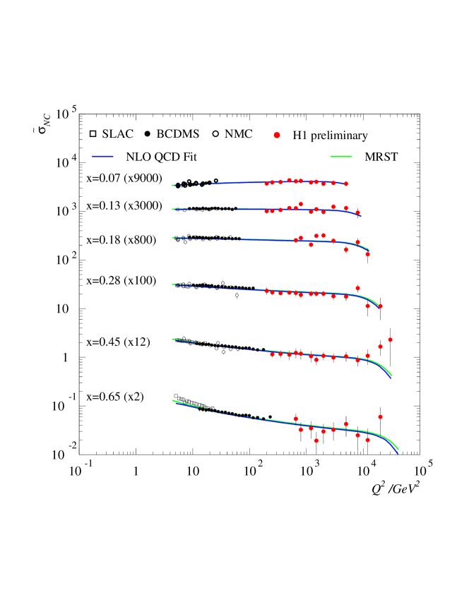
Fig. 51: The reduced neutral current cross section at high-$x$ compared with Standard Model predictions using the MRST parton density parameterization (lightly shaded line) and parton densities resulting from an H1 NLO QCD fit (solid line).

Recent data on the NC cross sections are shown in Fig. 51, where the preliminary data from H1 at large-$x$ for the reduced cross section

$$\tilde{\sigma}^{NC}\equiv\frac{xQ^{4}}{2\pi\alpha^{2}}\frac{1}{Y_{+}}\frac{d^{2}\sigma}{dxdQ^{2}}$$ (108)

are plotted as a function of $Q^{2}$. The cross sections presented now extend to $x=0.65$ and $Q^{2}=30,000$ GeV².

Fig. 52: The reduced charged current cross section compared with Standard Model predictions using the CTED4D parton density parameterization. The contributions of the PDF combination $\bar{u}+\bar{c}$ and $(1-y)^{2}(d+s)$ evaluated at leading order are shown by the dotted and dashed lines, respectively.

Preliminary double differential cross sections from the 1994-97 data are now also available for the CC reactions (?; ?). The results from the ZEUS collaboration are shown in Fig. 52. The results are again shown for the reduced cross section

$$\tilde{\sigma}^{CC}\equiv\frac{2\pi x}{G_{F}^{2}}\left(\frac{M_{W}^{2}+Q^{2}}{M_{W}^{2}}\right)^{2}\frac{d^{2}\sigma}{dxdQ^{2}}\;.$$ (109)

In LO, the reduced cross section is simply related to the following quark densities

$$\tilde{\sigma}^{CC}=(\bar{u}+\bar{c})+(1-y)^{2}(d+s)\;.$$ (110)

The separate contributions from the quarks and anti-quarks are shown in the figure. The quarks dominate at large-$x$, while the antiquark contribution is dominant at smaller $x$.

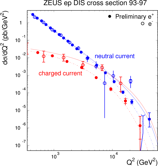
Fig. 53: The differential cross section versus $Q^{2}$ for neutral and charged current scattering as measured by ZEUS in the 1993-1997 data sets. The results are compared to Standard Model expectations separately for $e^{-}p$ and $e^{+}p$ scattering. The cross sections all become comparable near $Q^{2}=10000$ GeV², as expected from electroweak unification.

The single differential cross sections from ZEUS for both NC and CC scattering for the data through 1993-97 data are summarized in Fig. 53. As can be seen in this figure, the $e^{-}$ and $e^{+}$ cross sections at small $Q^{2}$ are very similar, as expected since photon exchange dominates this region. At higher $Q^{2}$, the expectation for the $e^{-}p$ cross section is higher than that for the $e^{+}p$ cross section as discussed above. The data are in agreement with the Standard Model within the experimental uncertainty. The CC cross sections for $e^{-}p$ are higher than for $e^{+}p$, as expected, and below the NC cross sections up to $Q^{2}\approx 10000$ GeV², at which point the cross sections become of comparable size. This is direct experimental evidence for electroweak unification. At this scale, the electromagnetic and weak interactions are of similar strength.

The two experiments H1 and ZEUS reported an excess of events above Standard Model expectations in February, 1997. This excess occurs at very large $Q^{2}>15000$ GeV², and will be discussed in section 8.7. This recent observation clearly emphasizes the importance of measurements in this previously unexplored kinematic regime.

5 Jet production

In QCD hadrons are composed of many quarks and gluons. When two hadrons collide at high energy, two partons can undergo a large angle scattering generating two or more final state partons at large momentum transverse to the initial beam direction. Each of the partons, released as a result of the hard scattering, will radiate more partons and evolve into a ”spray” of hadrons labeled as a jet. The nature of QCD radiation is such that the radiated partons, and subsequently the formed hadrons, will remain collimated around the original parton direction. This property is used to reconstruct the underlying partonic interaction.

The properties of jet production such as cross sections, transverse momentum distributions, angular distributions and jet shapes, are all sensitive to the properties of QCD and parton distributions in the interacting particles. This allows to study QCD at various levels and in various interactions.

In $ep$ interactions at HERA, jets can be produced as a result of a hard scattering between a quasi-real photon and the proton as well as from higher order QCD processes in deep inelastic scattering. While presumably there is a common denominator to all these processes, they are usually treated differently within perturbative QCD (pQCD) in order to improve the quality of the theoretical predictions. The guideline is set by the factorization theorem which prescribes which part of the cross section can be calculated within pQCD and which part is to be absorbed into the non-perturbative universal component. The general rule is that the perturbative process is the one which occurred at the hardest scale in the interaction.

Following this guideline, we will first discuss jet production in photoproduction and then in deep inelastic scattering. The subject is of great interest and very wide. Here we will only concentrate on some highlights typical of $ep$ scattering. For a full account, the interested reader is referred to two recent reviews (?; ?).

5.1 Defining the jets

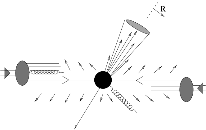
Fig. 54: A schematic representation of a hard scattering between two hadrons (from ?). The arrows represent the expected particle flow after the interaction. Hadrons produced as a result of fragmentation of one of the outgoing partons are contained within a cone of radius $R$.

Jets of particles, produced around partons emerging from the hard scattering, are accompanied by extra hadronic activity resulting from fragmentation (initial and final state parton radiation) and hadronization (hadron formation) of the spectator partons (see Fig. 54). This extra activity, both correlated and uncorrelated with the hard scattering, is called the underlying event. The underlying event consists primarily of low transverse momentum particles which overlap with the jets. As a result there is no unique way of assigning final state particles to the original partons. This is true both from the theoretical and experimental point of view. For quantitative measurements jets have to be somehow defined. This is achieved by constructing jet algorithms which prescribe how to combine hadrons close in phase space into jets. The experimental procedure has to match the theoretical calculations. There exist several jet algorithms and their use depends on particular applications.

5.1.1 Jet search algorithms

The jet search search algorithms are all based on the notion that particles emitted as a result of parton fragmentation and hadronization should be close to each other in phase space. The more sophisticated ones also take into account the dynamical features of parton radiation. In addition, since the underlying event is soft and particles have limited transverse momentum, the presence of jets will result in high transverse energy deposits. The variety of jet algorithms reflects the need to minimize hadronization effects, which cannot be taken into account in the theoretical calculations.

Cone algorithm

In the cone algorithm particles are combined in the pseudo-rapidity, $\eta$, and azimuthal angle, $\phi$, phase space. The variable $\eta=-\ln\tan\frac{\theta}{2}$ is defined through the angle $\theta$ relative to the interaction axis and $\phi$ is the angle around the interaction axis. All particles within a cone of radius R,

$$R=\sqrt{\Delta\eta^{2}+\Delta\phi^{2}}\leq R_{0}\,,$$ (111)

are combined into a jet of transverse energy $E_{T}$

$$E_{T}=\sum_{i}E_{Ti}\,,$$ (112)

where $i$ runs over all particles in the cone and $E_{Ti}=E_{i}\sin\theta_{i}$. The value of $R_{0}$ usually varies between $R_{0}=0.7$ to $R_{0}=1$. If the resulting $E_{T}$ is above a certain threshold the jet axis is defined by

$$\eta_{J} = \frac{1}{E_{T}}\sum_{i}E_{Ti}\eta_{i}\,,$$ (113)

$$\phi_{J} = \frac{1}{E_{T}}\sum_{i}E_{Ti}\phi_{i}\,.$$ (114)

In practice this procedure is applied on pair of particles and implies some number of iterations until the quantities defined in Eq. (112),( 113), (114) are stable with the jet cone remaining fixed.

The cone algorithm has an equivalent theoretical definition. Its advantage is that it can easily be applied to calorimetric measurements where energy deposits in calorimeter cells are treated as single particles. The cone algorithm was adopted as standard jet definition, called Snowmass Accord (?), because of its ease of implementation and reliable results at all orders in perturbation theory.

JADE algorithm

In the JADE algorithm (?) one defines for each pair of particles or clusters $i$ and $j$ the quantity,

$$y_{ij}=\frac{2E_{i}E_{j}(1-\cos\theta_{ij})}{W^{2}}\simeq\frac{m_{ij}}{W^{2}}\,,$$ (115)

where $m_{ij}$ is the invariant mass of the objects $i$ and $j$ and $W$ is the center-of-mass energy of the interaction. If $y_{ij}$ is smaller than a resolution parameter $y_{\mathrm{cut}}$ the objects are combined. The final set of jets is obtained when no further merging is possible. No requirement on $E_{T}$ of jets is applied. In the modified version of the algorithm, particularly suitable for deep inelastic scattering, the reference scale $W^{2}$ is replaced by $Q^{2}$. The number of jets found in an event depends on the $y_{\mathrm{cut}}$ parameter. This dependence is in principle predicted by the theory. In hadronic interactions the parent hadrons are included in the clustering as pseudo-particles. The jet containing the pseudo-particle is called the remnant jet.

$k_{T}$ algorithm

In the $k_{T}$ algorithm (?) it is the relative transverse momentum of two particles, rather than their invariant mass, that is used for clustering particles. Two particles, or at a later stage two clusters, $i$ and $j$ are merged if the transverse momentum, $k_{T}$, of the least energetic of the two objects is smaller than a predefined resolution scale, $k^{2}_{\mathrm{cut}}$,

$$k_{T}^{2}=2{\mathrm{min}}(E_{i}^{2},E_{j}^{2})(1-\cos\theta_{ij})<k^{2}_{\mathrm{cut}}\,.$$ (116)

In the original algorithm (?) which was designed for deep inelastic scattering $k^{2}_{\mathrm{cut}}=Q^{2}$. The treatment of the remnant jet is similar to the JADE algorithm. The $k_{T}$ algorithm is expected to be least affected by hadronization effects (?).

5.2 Jet production in photoproduction

One of the interests in studying jet production in photoproduction is to probe the hadronic nature of the photon. The photon is one of the gauge particles of the Standard Model and as such has no intrinsic structure. However it acquires a structure in its interactions with matter and in that sense it is a prototype for studying the formation of a partonic state.

In $ep$ scattering at HERA cross section considerations (see section 4.1) favor interactions with exchanged photon virtuality $Q^{2}\simeq 0$. These interactions can be treated as due to a convolution of a flux of quasi-real photons from the electron and the photon-proton interactions,

$$\frac{d\sigma_{ep}(y,Q^{2})}{dy}=\sigma_{\gamma p}(y)f_{\gamma/e}(y,Q^{2})\,,$$ (117)

where $f_{\gamma/e}$ denotes the photon flux. The photon flux is assumed to be given by the Weizsäcker-Williams approximation (?; ?). For a range $Q^{2}_{min}<Q^{2}<Q^{2}_{max}\ll 1\,\mathrm{GeV^{2}}$, the flux is given by

$$f_{\gamma/e}=\frac{\alpha}{2\pi}\left[\frac{1+(1-y)^{2}}{y}\ln\frac{Q^{2}_{max}}{Q^{2}_{min}}-2m_{e}^{2}\left(\frac{1}{Q^{2}_{min}}-\frac{1}{Q^{2}_{max}}\right)\right]\,.$$ (118)

5.2.1 Theoretical framework

In photon-nucleon interactions at low energies it was established that the photon behaves as if it fluctuated into a vector meson before interacting (for a review see ?). When QCD is turned on the variety of hadronic fluctuations of the photon increases, small and large partonic configurations can be formed, and their presence has implications for the interactions of the photon with hadronic matter.

The momentum distribution of partonic fluctuations of the photon can be measured directly in deep inelastic scattering of a lepton on a photon target. These measurement are performed in $e^{+}e^{-}$ colliders in which one of the electrons is the source of the probing photon and the other of the target photon. The notion of the photon structure function, and subsequently of parton distributions, can be consistently introduced.

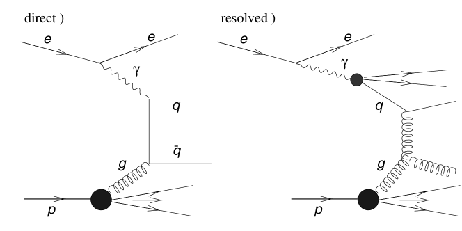
Fig. 55: Examples of diagrams which contribute to jet production in photoproduction: direct photon and resolved photon contributions as denoted in the figure.

Once the photon is replaced by a flux of partons, the QCD factorization theorem (?) can be applied to calculate cross sections for jet production in photon-proton interactions. These processes are called resolved photon processes. An example is shown in Fig. 55.

Partonic fluctuations of the photon in which the transverse momentum of the $q\bar{q}$ pair is larger than the virtuality of the probing photon are not included in the usual structure function formalism. They do however contribute to the jet production cross section and induce the direct photon processes. The name derives from the fact that these processes look as if the photon was probing directly the parton structure of the proton. This is depicted schematically in Fig. 55.

In summary, QCD predictions for photon proton interactions are based on two essential ingredients, the partonic nature of the photon and the underlying QCD hard subprocesses. We discuss them in more details below.

The photon structure function

The structure functions of the photon are defined in DIS $e\gamma\rightarrow eX$ through the interaction cross section,

$$\frac{d^{2}\sigma}{dxdQ^{2}}=\frac{2\pi\alpha^{2}}{xQ^{4}}\left[\left(1+(1-y)^{2}\right)F_{2}^{\gamma}-y^{2}F_{L}^{\gamma}\right]\,.$$ (119)

Fig. 56: Basic box diagram which contributes to the structure function of the photon in $\gamma^{*}\gamma$ collisions.

In the quark-parton model (QPM) the contribution to this cross section comes from the so called box diagram $\gamma^{*}\gamma\rightarrow q\bar{q}$ (see Fig. 56),

$$F_{2}^{\gamma}(x,Q^{2})=3\frac{\alpha}{\pi}\sum_{n_{f}}e^{4}_{q}x\left(x^{2}+(1-x)^{2}\right)\ln\frac{Q^{2}}{m^{2}_{q}}\,,$$ (120)

where $\alpha$ is the electromagnetic coupling constant, $e_{q}$ is the charge of quark $q$ in units of electron charge and $m_{q}$ is the mass of the quark. The sum runs over all active quark flavors, $n_{f}$.

Should this be the only contribution, the structure function of the photon would be fully calculable in QCD (?). In QCD, to leading order, the result (120) is preserved with the $m_{q}^{2}$ term replaced by the QCD cut-off parameter $\Lambda^{2}_{QCD}$. In the language of photon fluctuations the box diagram corresponds to rather symmetric $q\bar{q}$ fluctuations of the photon with a point-like coupling of quarks to the photon. The resulting contribution to the photon structure is called point-like or anomalous (as it does not appear for real hadrons). In reality the photon can fluctuate into more complicated partonic states and in particular into vector meson states. This generates a non-perturbative contribution to $F_{2}^{\gamma}$. Theoretically the two contributions cannot be disentangled. To parameterize $F_{2}^{\gamma}(x,Q^{2})$ it is therefore convenient, by analogy to the proton case, to define parton distributions in the photon and to use the DGLAP evolution equations, appropriately extended to the photon case (?; ?). The evolution equation for the quark density becomes inhomogeneous to account for the splitting of the photon into a $q\bar{q}$ pair. The latter is responsible for the fact that $F_{2}^{\gamma}(x,Q^{2})$ is large at large $x$ and increases with $Q^{2}$ at any value of $x$.

Experimentally $F_{2}^{\gamma}$ is measured in $e^{+}e^{-}$ interactions, by requiring that one of the electrons scatters under small angles and remains undetected (the source of the target photon) while the second one scatters under a large angle, providing the probing virtual photon.

Fig. 57: The structure function of the photon $F_{2}^{\gamma}/\alpha$ as a function of $x$ for various $Q^{2}$ values as denoted in the figure (taken from ?. The symbols correspond to measurements in $e^{+}e^{-}$ interactions. Two selected parton parameterizations are also shown: GRV (?) (full line) and SaS (?) (dashed line).

The $x$ dependence of $F_{2}^{\gamma}$ in bins of $Q^{2}$ is shown in Fig. 57. For the sake of comparison with the proton structure function the scale of $x$ was chosen logarithmic. The measurements are compared to two commonly used sets of parton distributions in the photon (?; ?). At higher $x$, where data are available, all the parameterizations describe $F_{2}^{\gamma}$ well. The largest differences are seen at low $x$, where gluons play an important role. The uncertainty in the gluon content of the photon is thought to be worse than for the proton since no momentum sum rule is used to constrain the gluon distribution. Recently such a sum rule has been derived (?). The uncertainty in the gluon distribution can be partly reduced by the hard photoproduction data from the HERA experiments.

It is of interest to consider what happens to the photon structure function when the virtuality increases. We will denote by $P^{2}$ the virtuality of the photon and keep $Q^{2}$ to denote the scale at which the virtual photon is probed. It has been shown (?; ?) that in the limit $\Lambda^{2}_{QCD}\ll P^{2}\ll Q^{2}$ the virtual photon structure function can be calculated in QCD. The result is similar to the QPM result (120) with the mass of the quark replaced by the virtuality of the photon,

$$F_{2}^{\gamma^{*}}(x,Q^{2},P^{2})=3\frac{\alpha}{\pi}\sum_{n_{f}}e^{4}_{q}x\left(x^{2}+(1-x)^{2}\right)\ln\frac{Q^{2}}{P^{2}}\,.$$ (121)

The details of how the non-perturbative part behaves with $P^{2}$ cannot be calculated in QCD. One can only speculate that its contribution disappears faster with increasing $P^{2}$ than the point-like part. However the non-perturbative contributions to the photon structure may remain sizeable up to $P^{2}=1\,\mathrm{GeV^{2}}$ (?).

Predictions of perturbative QCD

In leading order of perturbative QCD, jet production in photon-proton interactions is attributed to two hard processes, called the direct and the resolved photon processes. The calculation of the cross sections is based on the QCD factorization theorem (?). It allows to decompose (factorize) the calculation into the cross section for the elementary hard subprocess, calculable in QCD, and fluxes of partons entering the hard scattering. The hard scale in the interaction is provided by the transverse momenta of the outgoing partons. For the production of two jets with transverse momentum $p_{T}$, the $\gamma p$ cross section can be written symbolically as

$$\sigma_{\gamma p}(p_{T}^{2},W)=\sum_{i,j}\sum_{k,l}f_{i/\gamma}(x_{\gamma},p_{T}^{2})f_{j/p}(x_{p},p_{T}^{2})\hat{\sigma}(i+j\rightarrow k+l)(p_{T}^{2},\hat{s})\,,$$ (122)

where $x_{\gamma}$ and $x_{p}$ denote the fraction of the photon and proton momentum carried by the interacting partons and $\hat{s}=x_{\gamma}x_{p}W^{2}$ with $W$ the center-of-mass energy of the $\gamma p$ interaction. An implicit integration over $x_{\gamma}$ and $x_{p}$ is assumed.

For resolved photon processes the hard scattering is modeled as taking place between a parton in the photon and a parton in the proton (see Fig. 55). Many elementary processes contribute to this cross section. A quark or a gluon from the photon may interact with a quark or a gluon in the proton. In the final state we expect two back-to-back jets, this time accompanied by the remnants of the proton and of the photon.

In direct photon processes it is convenient to view the hard scattering as occurring between the photon and a parton from the proton (see Fig. 55). In formula (122) parton $i$ is replaced by a photon and $f_{\gamma/\gamma}(x_{\gamma})=\delta(1-x_{\gamma})$. The process $\gamma q\rightarrow qg$ is called QCD Compton scattering (QCDC), while $\gamma g\rightarrow q\bar{q}$ is called boson-gluon fusion (BGF). In leading order we expect the final state to consist of two back-to-back jets and the remnant of the proton.

When higher order QCD corrections are included, extra hard parton radiation is present and the division of photon induced processes into direct and resolved is no longer possible. However, it is always possible to enhance one of the contributions because the direct photon contribution is expected to dominate at $x_{\gamma}\simeq 1$ while the resolved processes are expected at lower $x_{\gamma}$.

The parton densities in the proton are well constrained by other measurements (see section 4.3), so that photoproduction of jets can be used to constrain the parton content in the photon.

5.2.2 pre-Hera results

Little was known experimentally about hard scattering in photoproduction before HERA data became available. The first indication for the presence of hard scattering, in excess of what would be expected if the photon were just a meson, was observed by the NA14 experiment at CERN (?). A similar excess was observed later by the WA69 experiment at CERN (?) at a center-of-mass energy $\sqrt{s_{\gamma p}}=18\,\mathrm{GeV}$. In both cases the excess was assigned to the direct photon contribution. The presence of the resolved photon component could not be established.

The first experimental evidence for the presence of a hard resolved photon component was reported by the AMY experiment (?), based on the study of the hadronic final states in $\gamma\gamma$ interactions at $4<\sqrt{s_{\gamma\gamma}}<20\,\mathrm{GeV}$.

5.2.3 Selection of HERA results

The production of events with large transverse energy in $\gamma p$ interactions has been extensively studied at HERA. The concept of resolved and direct photon contributions as well as the validity of the QCD approach to photoproduction have been fully confirmed. First attempts have been made to constrain the parton distributions in the photon. After discussing the kinematic reconstruction of hard photoproduction events, we describe these results below.

Event kinematics

The experimental signature for photoproduction events is either the presence of an electron scattered under a very small angle in the luminosity detector (tagged photoproduction with $Q^{2}<10^{-2}\,\mathrm{GeV^{2}}$) or the lack of the scattered electron in the main HERA detectors (untagged photoproduction, $Q^{2}<4\,\mathrm{GeV^{2}}$ and $\langle Q^{2}\rangle\simeq 10^{-3}\,\mathrm{GeV^{2}}$). Hard photoproduction events are selected by requiring that the total transverse energy $E_{T}$ in the event, measured with respect to the beam axis, be large (typically $E_{T}>10\,\mathrm{GeV}$).

For tagged photoproduction, the center-of-mass energy of the $\gamma p$ interaction is obtained using the initial, $E_{e}$, and the scattered electron, $E_{e}^{\prime}$, energies,

$$W^{2}=y_{el}s=\left(1-\frac{E_{e}^{\prime}}{E_{e}}\right)s\,.$$ (123)

In the untagged photoproduction $W$ is determined using the hadronic final state,

$$W^{2}=y_{\scriptscriptstyle JB}s=\frac{\sum_{i}(E_{i}-p_{zi})}{2E_{e}}s\,,$$ (124)

where the sum runs over all the objects (particles and/or clusters) reconstructed in the detector.

To describe the event kinematics we define $x_{\gamma}$ as the fraction of the photon momentum, $q$, and $x_{p}$ as that of the proton, $P$, carried by the partons initiating the hard scattering. We denote by $p_{1}$ and $p_{2}$ the four-momenta of the scattered partons. For a two body process we expect,

$$x_{\gamma}q+x_{p}p=p_{1}+p_{2}\,,$$ (125)

By multiplying (scalar product) both sides, once by $P$ and once by $q$ and manipulating the two equations, we obtain

$$x_{\gamma} = \frac{(p_{1}+p_{2})\cdot P}{q\cdot P}\,,$$ (126)

$$x_{p} = \frac{(p_{1}+p_{2})\cdot q}{q\cdot P}\,,$$ (127)

where the approximation, $q^{2}=0$ and $P^{2}=0$ was made. This approximation holds well for high energy photoproduction. Another representation, more convenient for measurements, is through the transverse momentum, $p_{Ti}$, and the pseudo-rapidity, $\eta_{i}$, of the partons,

$$x_{\gamma} = \frac{\sum_{i=1,2}p_{Ti}e^{-\eta_{i}}}{2yE_{e}}\,,$$ (128)

$$x_{p} = \frac{\sum_{i=1,2}p_{Ti}e^{\eta_{i}}}{2E_{p}}\,.$$ (129)

Since variables defined at the parton level are not observables, experimental estimators are introduced, $x_{\gamma}^{\scriptscriptstyle\mathrm{OBS}}$, and $x_{p}^{\scriptscriptstyle\mathrm{OBS}}$. In the first step a jet algorithm is applied. For a cluster of particles to be defined as a jet, its transverse energy relative to the interaction axis, is required to be typically $E_{T}^{jet}>4\,\mathrm{GeV}$. To determine $x_{\gamma}^{\scriptscriptstyle\mathrm{OBS}}$ or $x_{p}^{\scriptscriptstyle\mathrm{OBS}}$ at least two jets are required. If more than two jets are found in an event, usually the two with the highest transverse energy are used. The variables $x_{\gamma}^{\scriptscriptstyle\mathrm{OBS}}$ and $x_{p}^{\scriptscriptstyle\mathrm{OBS}}$ are determined using formulae (128) and (129), after replacing the $p_{T}$ and $\eta$ of the partons by the corresponding jet variables which are $E_{T}^{\mathrm{jet}}$ and $\eta^{\mathrm{jet}}$ as determined from the jet algorithm (see section 5.1.1).

The resolved and direct components

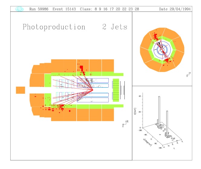
Fig. 58: Example of a photoproduction event presumably mediated by a direct photon as seen in the H1 detector. The electrons come from the left, the protons from the right. Two jets are clearly seen. There is no activity to the right of the detector, the presumed direction of the emitted photon.

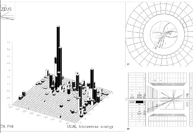
Fig. 59: Example of a photoproduction event due to a resolved photon, as seen in the ZEUS detector. The electrons come from the left, the protons from the right. In addition to the proton remnant, there is clear jet structure. Most likely, the jet at smallest $\eta$ is the photon remnant.

Jet production in photoproduction was established for the first time by the HERA experiments (?; ?). The jet structure in the events can be seen by eye. An example of a direct photon event is shown in Fig. 58. Two jets in the detector are clearly seen and there is no activity in the rear region which corresponds to the photon fragmentation, as if the whole photon was absorbed in the interaction. In Fig. 59 a resolved photon event is shown. A third jet with much less transverse energy is seen in the rear detector - this is the remnant of the photon.

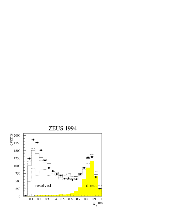
Fig. 60: $x_{\gamma}^{\scriptscriptstyle\mathrm{OBS}}$ distribution for jets with $E_{T}^{\mathrm{jet}}>6$ GeV, $-1.375<\eta^{\mathrm{jet}}<1.875$, where $x_{\gamma}^{\scriptscriptstyle\mathrm{OBS}}$ is calculated using corrected variables. The data (black dots) are compared to the results of the HERWIG MC model with multiple interactions (solid line) and without (dotted line) and PYTHIA MC model with multiple interactions (dashed line). The shaded area represents the direct photon contribution expected in the HERWIG MC model.

The $x_{\gamma}^{\scriptscriptstyle\mathrm{OBS}}$ distribution measured for a sample of di-jet events with $E_{T}^{\mathrm{jet}}>6\,\mathrm{GeV}$ and $-1.375<\eta^{\mathrm{jet}}<1.875$ is shown in Fig. 60 (?). The events dominated by the direct photon processes cluster at large $x_{\gamma}^{\scriptscriptstyle\mathrm{OBS}}$. A clear peak of events with $x_{\gamma}^{\scriptscriptstyle\mathrm{OBS}}>0.75$ is observed and the distribution is well reproduced by a MC model of direct photon processes (HERWIG (?)). The majority of events have $x_{\gamma}^{\scriptscriptstyle\mathrm{OBS}}<0.75$ and are attributed to the resolved photon processes. MC models which include the simulation of both processes at leading order of QCD and include in addition multiple interactions reproduce the overall shape of the data but fail to describe the small $x_{\gamma}^{\scriptscriptstyle\mathrm{OBS}}$ region.

Fig. 61: (a) Pseudorapidity, $\eta_{3}$, distribution of the third, lowest transverse momentum jet in a three jet event. (b) The transverse momentum distribution of that jet, $p_{T3}$, if $\eta_{3}<-1.0$. The data are compared to the expectations of two approaches in the PYTHIA MC model: in one, the intrinsic transverse momentum of partons in the photon is negligible (solid line), in the other, a power like dependence is assumed (dotted line).

The properties of the photon remnant have been studied by the ZEUS experiment (?). The $k_{T}$ cluster algorithm was used to decompose the event into three jets. If two jets had transverse energy $E_{T}^{\mathrm{jet}}>6\,\mathrm{GeV}$ and rapidities well into the forward region, the third cluster on average was found in the photon fragmentation region as shown in Fig. 61a. The two leading jets were interpreted as due to the hard scattering, while the third jet was interpreted as originating from the photon remnant. The third jet was found to be well collimated, with a relatively large transverse momentum, as can be seem in Fig. 61b. This is in contrast with expectations for hadron-hadron interactions where the remnants (with spectator partons) remain with low transverse momenta. However, the anomalous component of the photon structure, which is due to small size configurations, leads to initial partons with relatively large transverse momenta. The requirement of the presence of three jet-like structure favors events from the anomalous photon fluctuation. Note that the average transverse energy of the third jet remains low compared to $E_{T}^{jet}$ of the two leading jets (see Fig. 61b).

Angular distributions

The angular distribution of the jets in their center-of-mass system reflects the underlying parton dynamics. To leading order in QCD, the direct photon processes proceed via either boson-gluon fusion or QCD Compton scattering. These processes involve a quark propagator in the $s$, $t$ or $u$ channel, with $t$ and $u$ channel processes dominating. In resolved processes the dominant subprocesses, e.g. $qg\rightarrow qg$, $gg\rightarrow gg$ and $qq\rightarrow qq$, have $t$-channel gluon exchange diagrams.

The angular dependence of the cross section for resolved processes with a spin-1 gluon propagator is approximately $\propto(1-|\cos\theta^{\ast}|)^{-2}$ (as in Rutherford scattering), where $\theta^{\ast}$ is the scattering angle of one of the jets in their center-of-mass. This cross section rises more steeply with increasing $|\cos\theta^{\ast}|$ than that for direct processes with a spin-$\frac{1}{2}$ quark propagator, where the angular dependence is approximately $\propto(1-|\cos\theta^{\ast}|)^{-1}$. After inclusion of all LO diagrams, QCD predicts that the angular distribution of the outgoing partons in resolved processes will be enhanced at large $|\cos\theta^{\ast}|$ with respect to direct photon processes. This property is expected to be preserved in next-to-leading order (NLO) calculations (?).

Fig. 62: The cross section $d\sigma/d|\cos\theta^{*}|$ normalized to one at center-of-mass scattering angle $\theta^{*}=90^{o}$, for resolved (black dots) and direct (open circles) photoproduction. The data are compared to (a) NLO and LO QCD calculations as well as (b) expectations of the HERWIG and PYTHIA MC models.

By dividing dijet events into samples with $x_{\gamma}^{\scriptscriptstyle\mathrm{OBS}}>0.75$ and $x_{\gamma}^{\scriptscriptstyle\mathrm{OBS}}<0.75$ it is possible to obtain samples enriched in direct and resolved processes respectively (?). The $\cos\theta^{\ast}$ distributions thus obtained are shown in Fig. 62. The resolved photon processes have as expected a steeper angular distribution than the direct processes. The distribution is well reproduced by LO and NLO QCD calculations as well as MC models.

Structure of the real photon

The measured jet production cross section can be confronted with QCD expectations. These depend on the momentum distribution of partons in the photon and in the proton (see Eq. (122)). The procedure for unfolding the parton distributions is not as simple as in the case of deep inelastic scattering. The measured cross section is determined at the hadron level and the information on the hard scattering process is obscured by higher order QCD radiation and hadronization effects. It may further be obscured by the presence of other hard scatters occurring in the same event (?). From a purely probabilistic approach, parton densities in the HERA kinematic regime are high enough so that the chance for more than one scatter in an event becomes significant (?).

Fig. 63: The inclusive dijet cross section as a function of the squared jet transverse energy $(E_{T}^{\mathrm{j}ets})^{2}$ for ranges of the reconstructed parton fractional energy $x_{\gamma}^{\mathrm{j}ets}$ as denoted in the figure. The data are compared to NLO QCD calculations for two parameterizations of parton densities in the photon, GRV (?) and GS (?). Also shown is the expectation of the PYTHIA MC model in which the LO order GRV parameterization was used.

The additional effects can be modeled within a particular MC generator and if a good description of the data is achieved , then, within this particular model, the correlation between the partons from the hard scattering and the jets can be established. One can then deduce what parton distributions in the photon are needed to successfully describe the observed jet rates. This procedure was carried out by the H1 experiment (?). The measured inclusive dijet cross section as a function of $(E_{T}^{jet})^{2}$ and $x_{\gamma}$ is very well reproduced by the PYTHIA MC model (?) used to unfold the parton densities, as shown in Fig. 63. It is also in good agreement with NLO QCD calculations (?).

Fig. 64: Leading order effective parton distribution of the photon $x_{\gamma}\bar{f}_{\gamma}(x_{\gamma},p_{T}^{2})=x_{\gamma}(f_{q/\gamma}(x_{\gamma},p_{T}^{2})+9/4f_{9/\gamma}(x_{\gamma},p_{T}^{2}))$, divided by the fine structure constant $\alpha$, shown as a function of the squared parton transverse momentum $p_{T}^{2}$ for two ranges of the parton fractional energy $x_{\gamma}$. The full line represents the equivalent function derived from the LO GRV parameterization of the photon structure function. Also shown are the contribution of the quark component alone (dotted line) and the expectation if the photon was a meson (dashed line - VDM).

The effective parton distributions were unfolded from the cross section in two bins of $x_{\gamma}$ as a function of the hard scattering scale, assumed to be $p_{T}^{2}$ of the jets. The result is shown in Fig. 64 and compared to the expectations of the GRV (?) parameterization. As predicted for the photon case, parton densities rise with increasing $p_{T}^{2}$ both for medium and large $x_{\gamma}$.

Since the calculation is carried out at leading order it is possible to disentangle the various contributions. This is also shown in the figure. The non-perturbative part of the photon structure, expected to contribute at small $x_{\gamma}$ constitutes only a small fraction of parton densities for $x_{\gamma}>0.2$. The quark component of the photon is not sufficient to explain the observed effective parton densities, a substantial contribution of gluons is necessary.

Structure of the virtual photon

The more the photon is off-shell the more likely it becomes that its coupling to quarks becomes point-like. The structure function of the photon can then be calculated in QPM and QCD (?; ?). The expectation is that in hard photoproduction induced by a virtual photon, the hadronic contribution will decrease and the resolved photon processes will be suppressed compared to the direct photon processes (?; ?; ?).

At large virtuality of the photon, we move into the deep inelastic scattering regime, $Q^{2}$ becomes the largest scale in the interaction, and application of the factorization theorem leads to viewing the scattering as due to direct photon coupling to the quarks in the proton. However if, as a result of QCD Compton or BGF processes, jets are produced with transverse energy squared $(E_{T}^{\mathrm{jet}})^{2}>Q^{2}$, the largest scale will be in the hard scatter leading to jets and the photon, once again, will develop a partonic structure (?; ?; ?). This apparent contradiction is in fact simple to understand; the perturbative QCD evolution formalism applied to the proton structure function does not include the region $E_{T}^{2}>Q^{2}$. Their contribution to the total DIS cross section is assumed to be negligible.

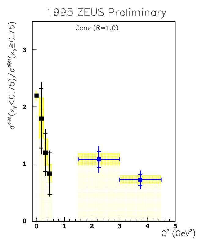
Fig. 65: The ratio of resolved to direct photon cross sections, $\sigma_{R}/\sigma_{D}$, as a function of photon virtuality $Q^{2}$. The shaded bands represent the systematic error due to jet energy scale uncertainties.

The ZEUS experiment has studied dijet production in virtual photon-proton scattering in three $Q^{2}$ ranges, $Q^{2}\simeq 0\,\mathrm{GeV^{2}}$ (untagged $\gamma p$), $0.1<Q^{2}<0.7\,\mathrm{GeV^{2}}$ ($e$ tagged in the BPC) and $1.5<Q^{2}<4.5\,\mathrm{GeV^{2}}$ ($e$ tagged in the UCAL) (?). The jets were required to have $E_{T}^{\mathrm{jet}}>6.5\,\mathrm{GeV}$ and $-1.125<\eta^{\mathrm{jet}}<1.875$. In each $Q^{2}$ range the sample was divided into events with $x_{\gamma}^{\scriptscriptstyle\mathrm{OBS}}>0.75$ (direct) and $x_{\gamma}^{\scriptscriptstyle\mathrm{OBS}}<0.75$ (resolved). The ratio of resolved over direct dijet cross sections was measured as a function of $Q^{2}$ and is shown in Fig. 65. As expected, the fraction of events dominated by resolved photon processes decreases relative to the direct photon ones as a function of $Q^{2}$. This trend is not reproduced by a MC model in which no $Q^{2}$ dependence of the parton distributions in the photon is assumed.

Fig. 66: The inclusive $\gamma^{*}p$ jet cross section $\sigma_{\gamma^{*}p}(Q^{2})$ as a function of $Q^{2}$, for jets with transverse energy $E_{T}^{*}$, measured in the $\gamma^{*}p$ system, as denoted in the figure. The lines correspond to expectations from two MC models for final states in DIS, LEPTO (solid line) and ARIADNE (dashed line).

Fig. 67: The inclusive $\gamma^{*}p$ jet cross section $\sigma_{\gamma^{*}p}(Q^{2})$ as a function of $Q^{2}$, for jets with transverse energy $E_{T}^{*}$, measured in the $\gamma^{*}p$ system, as denoted in the figure. The lines correspond to expectations from MC models (as shown in the figure) in which the virtual photon induces direct and resolved processes. Different parameterizations of the virtual photon structure function are shown. Also shown is the expectation if the structure of the virtual photon would not be suppressed with increasing $Q^{2}$.

The H1 analysis (?) covers the range $0<Q^{2}<49\,\mathrm{GeV^{2}}$ and $0.3<y<0.6$. The inclusive cross section for jet production with $E_{T}^{\mathrm{jet}}>4\,\mathrm{GeV}$ was studied as a function of $Q^{2}$ and compared with MC models with and without structure assigned to the virtual photon. As seen in Fig. 66, models such as ARIADNE and LEPTO, which describe well the inclusive features of deep inelastic scattering, fail to reproduce the cross section when $(E_{T}^{\mathrm{jet}})^{2}>Q^{2}$. However, as shown in Fig. 67, models (?; ?) in which a photon structure, dependent on its virtuality, is assumed, reproduce the data very well. This observation establishes contributions to $ep$ scattering cross section, which are not taken into account in the perturbative expansion up to NLO. In fact, for $Q^{2}>10\,\mathrm{GeV^{2}}$, H1 has observed that the production rate of dijets with $(E_{T}^{\mathrm{jet}})^{2}\geq Q^{2}$ is well reproduced by QCD calculations in which the jet cross section is evaluated up to NLO (?).

In summary, HERA results have established that even a virtual photon develops a hadronic structure when probed at a scale larger than its virtuality.

5.3 Jet production in deep inelastic scattering

Jet production in deep inelastic scattering is the manifestation of QCD beyond leading order approximation and therefore a sensitive probe of QCD dynamics. At HERA, clean jet structures can develop thanks to the large available phase space. There are many features of jet production in deep inelastic scattering which are important for understanding perturbative and non-perturbative aspects of QCD. Here we will concentrate on those aspects which make HERA unique.

5.3.1 Theoretical framework

Jets in DIS result from the scattered quark and from QCD radiation. The rates of jet production can be calculated in QCD and depend on the parton densities in the proton as well as on the value of the strong coupling constant $\alpha_{s}$. The pattern of radiation depends on the details of the evolution dynamics in QCD and can be exploited in searching for deviations from the DGLAP evolution. This is particularly important at small $x$ when many radiation steps have to be integrated over.

Higher order QCD processes

Multi-jet production rates are at the present the only features of DIS final states that have been fully predicted in perturbative QCD. In leading order of QCD, jet production in DIS is due to QCD Compton scattering (QCDC) and boson-gluon fusion (BGF) (see Fig. 10). The corresponding diagrams are the same as for direct photon processes (see Fig. 55). The cross section for the production of jets have been calculated in QCD up to NLO (?; ?; ?; ?).

The cross section for the production of $n$ jets plus the remnant, $\sigma_{n+1}$, can be represented as

$$\sigma_{n+1}(x,Q^{2};y_{\mathrm{cut}})=\alpha_{s}^{n-1}(Q^{2})A_{n}(x,Q^{2};y_{\mathrm{cut}})+\alpha_{s}^{n}(Q^{2})B_{n}(x,Q^{2};y_{\mathrm{cut}})+\ldots\,,$$ (130)

where $A_{n}$ and $B_{n}$ are calculable in terms of parton distribution functions of the proton. Here $y_{\mathrm{cut}}$ denotes the resolution parameter used in the jet algorithm. Measurements of jet rates provide a method to determine the strong coupling constant.

The QCDC and BGF processes result in the presence of two jets in the hadronic final state, in addition to the proton remnant. At HERA, the rate of two-jet production is used to measure $\alpha_{s}$ as a function of $Q^{2}$. QCDC scattering depends on the quark densities in the proton. The BGF process is sensitive to the gluon content of the proton. Schematically,

$$\sigma_{2+1}=\alpha_{s}(Q^{2})\left[A_{{}_{\mathrm{QCDC}}}q(x_{q/p},Q^{2})+A_{{}_{\mathrm{BGF}}}g(x_{g/p},Q^{2})\right]\,,$$ (131)

where $x_{q/p}$ and $x_{g/p}$ are the fractional momenta carried by the incoming quark and gluon respectively. Since the quark distributions are well constrained by the measurements of the $F_{2}$ structure function (see section 4.3) the two-jet production cross section can be used to unfold the gluon distribution in the proton.

The main uncertainty in confronting experimental data with theory stems from hadronization effects which cannot be calculated perturbatively.

BFKL dynamics

The main difference between the BFKL evolution and the DGLAP evolution is in the pattern of radiation assumed to be dominant in parton evolution. The process of parton evolution can be schematically represented by the diagram of Fig. 9. The distance in rapidity space of parton $i$ relative to the proton can be expressed as

$$\Delta y_{i}=y_{p}-y_{i}=\ln\frac{2E_{p}}{m_{p}}-\ln\frac{2x_{i}E_{p}}{k_{Ti}}\sim\ln\frac{1}{x_{i}}\,,$$ (132)

where $E_{p}$ is the energy and $m_{p}$ the mass of the proton. Here $x_{i}$ denotes the fraction of the proton momentum carried by the $i$-th parton and $k_{Ti}$ is its transverse momentum relative to the proton.

The evolution equations derived in perturbative QCD are meant to describe the $Q^{2}$ dependence of global quantities such as the DIS cross section. It is however believed that also the final states will remember the radiation pattern which leads to evolution. This is introduced in MC models such as LEPTO (?) or HERWIG (?).

In the DGLAP evolution, the strong ordering in transverse momenta (relative to the proton beam) $k_{T1}<k_{T2}<\ldots<k_{Tn}\simeq Q$ of the subsequent radiation requires that partons with the highest $k_{T}$ be radiated close to the photon absorption point. The QCDC and BGF processes are the results of such an evolution. Close to the proton, the partons are expected to have small $k_{T}$. In the BFKL evolution, no ordering in $k_{T}$ is implied and one expects an enhanced parton activity in the central and forward region, between the current system and the proton remnant.

Assuming parton-hadron duality (?), deviations from the DGLAP evolution would result in an increase of the transverse energy in the central rapidity range (?; ?). It should also be possible to observe jets with $k_{t}\simeq Q$ for large $x_{i}$ (?; ?; ?), which are not allowed in the DGLAP evolution. In fact the rate of such jets, if they exist, should be enhanced for small Bjorken $x$ since in the BFKL approach, at least to leading order, the cross section is expected to rise very fast ($\sigma\sim(x/x_{i})^{-0.5}$) (?).

To summarize, the footprint of BFKL dynamics should manifest itself in partons in the final state with transverse momenta larger than expected from the DGLAP evolution. Assuming duality between partons and hadrons the same effects should be present in the hadronic final state. Furthermore the rate of jet production with large fraction of the proton momentum should be enhanced for small-$x$ DIS.

One of the problems encountered in looking for BFKL symptoms in the final states is the lack of MC models for hadron production which incorporate fully the BFKL dynamics. The predictions that exist are calculated at the parton level and the effect of hadronization, which may be strong, precludes direct comparisons with BFKL based calculations.

The data are usually compared to three MC models of hadronic final states in DIS. Leading log DGLAP parton showers are implemented in the LEPTO (?) and HERWIG (?) generators. The main difference in the two generators is in the hadronization stage. The ARIADNE generator (?) parton showers are generated as a result of radiation from color dipoles formed by the color charges after the interaction. The gluons emitted by the dipoles do not obey strong ordering in $k_{T}$. All of these MC generators provide a satisfactory overall description of current DIS final state data (?).

5.3.2 Selection of HERA results

From the multitude of studies which are carried out for the hadronic final states in DIS (?), we report here on the study of jets shapes, the determination of $\alpha_{s}$ and on the search for the BFKL dynamics.

Jet shapes

The internal structure of jets is expected to depend on the type of primary parton, quark or gluon, from which the hadronic jet evolved. The formation of a jet from a parton is driven mainly by gluon emission. As a consequence of a larger gluon-gluon coupling strength compared to that of quark-gluon coupling, the gluon jets are expected to be broader than quark jets. This expectation can be tested by comparing jet shapes in different reactions in which in the final state jets are predominantly initiated by quarks or gluons.

At HERA, in deep inelastic neutral and charged current scattering, the dominant jet production mechanism is that of one quark jet. The same is true for $e^{+}e^{-}$ annihilation. In $p\bar{p}$ and $\gamma p$ scattering gluon initiated jets are expected to give a substantial contribution.

Most suitable for jet shape studies is the cone algorithm in which relatively little is assumed about the energy flow within a cone of radius $R=1$ in the pseudo-rapidity $\eta$ and azimuthal angle $\phi$ space.

The integrated jet shape, $\psi(r)$ is defined by

$$\psi(r)=\frac{1}{N_{jets}}\sum_{jets}\frac{E_{T}(r)}{E_{T}(R)}\,,$$ (133)

where $E_{T}(r)$ denotes the transverse energy contained in a cone of radius $r$ around the axis of the jet and $N_{jets}$ is the total number of jets in the sample. By definition $\psi(R)=1$.

Fig. 68: Integrated jet shape $\psi$ at a fixed value of $r=0.5$, as a function of $\eta^{\mathrm{jet}}$ (upper plot) and $E_{T}^{\mathrm{jet}}$ (lower plot) in neutral current DIS at $Q^{2}>100\,\mathrm{GeV^{2}}$. The expectations of different MC models are shown for comparison.

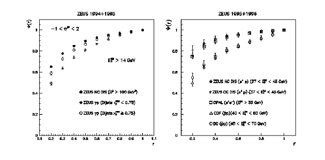
Fig. 69: Integrated jet shape $\psi$ as function of the radius of integration $r$, in neutral current DIS at $Q^{2}>100\,\mathrm{GeV^{2}}$ compared to jet shapes in direct and resolved photoproduction (left plot). Comparison between jet shapes in neutral current, charged current DIS and $e^{+}e^{-}$ and $p\bar{p}$ interactions (right plot).

The integrated jet shape $\psi(0.5)$ for jets found in neutral current DIS at $Q^{2}>100\,\mathrm{GeV^{2}}$, with $E_{T}^{jet}>14\,\mathrm{GeV}$ and $-1<\eta^{jet}<2$ (?), is shown in Fig. 68. The jet shape does not depend on $\eta^{jet}$, but the jets become more collimated as $E_{T}^{jet}$ increases. For jets with $E_{T}^{jet}\simeq 40\,\mathrm{GeV}$, almost $95\%$ of the transverse energy is contained within a cone of radius $r=0.5$.

When compared to jets seen in hard photoproduction, the NC jets are found to be more collimated as shown in Fig. 69. The difference between jet shapes in processes dominated by direct photon and resolved photon processes is also apparent in the figure. The latter are dominated by production of gluon jets.

In Fig. 69 the jet shapes are compared for various processes. The jets in NC, CC DIS and in $e^{+}e^{-}$ (?) interactions, which are predominantly initiated by quarks are less broad than jets with similar $E_{T}^{jet}$ measured in $p\bar{p}$ experiments (?; ?).

These observations confirm the expectation that gluon initiated jets are broader than quark initiated jets. The similarity in the jet shapes also indicates that the pattern of QCD radiation close to the primary parton is to a large extent independent of the hard scattering process.

Measurements of $\alpha_{s}$

The strong coupling constant $\alpha_{s}$ is a fundamental parameter of the Standard Model and the measurement of its value in different reactions, sensitive to different aspects of the theory, is of utmost importance. At HERA, $\alpha_{s}$ can be extracted in several ways, as outlined below.

The decrease in the quark densities at large $x$ with increasing scale $Q^{2}$ is understood in QCD as due to the radiation of gluons from the quarks. A measurement of the scaling violations therefore yields information on $\alpha_{s}$. Fixed target DIS experiments have extracted $\alpha_{s}$ via this method and have achieved very precise results ($\delta_{exp}\alpha_{s}=0.003$). At small $x$, where HERA structure function measurements have been performed, the scaling violations depend not just on $\alpha_{s}$ but also on the gluon density in the proton (the number of quarks increase due to the process $g\rightarrow q\bar{q}$). A combined analysis is quite difficult, and will require much larger data sets and considerably smaller systematic errors than are currently available. The extraction of $\alpha_{s}$ at large-$x$ values is statistically limited.

It should be noted that $\alpha_{s}$ can be extracted in the context of different QCD based models. For instance, in the double asymptotic scaling approach (?; ?), $\alpha_{s}$ appears as a parameter but the gluon density does not. A fit to the H1 data (?) with this model yields

$$\alpha_{s}(M_{Z})=0.113\pm 0.002\pm 0.006\;.$$ (134)

This method yields very small errors, but the theoretical uncertainties must still be worked out.

Dijet production in DIS proceeds in LO via QCDC scattering or BGF, as depicted in Fig. 10. The matrix elements for these processes have been calculated in NLO, and the rates for dijet events can be compared to expectations to extract $\alpha_{s}$. It is imperative to use calculations at least at NLO to reduce uncertainties due to different scales (factorization, renormalization).

A measurement of the rate of dijet events to single jet events as a function of $y_{\mathrm{cut}}$, the resolution parameter in the jet definition, is sensitive to the value of $\alpha_{s}$ (see Eq. (131)). In NLO the dijet rate can be expressed as

$$R_{2+1}(Q^{2},y_{c}) = \frac{\sigma_{2+1}(Q^{2},y_{c})}{\sigma_{tot}(Q^{2})}$$ (135)

$$= a(Q^{2},y_{c})\alpha_{s}(Q^{2})+b(Q^{2},y_{c})\alpha_{s}^{2}(Q^{2})\,,$$ (136)

where $y_{c}=y_{\mathrm{cut}}$ and the coefficients $a$ and $b$ are given by perturbation theory.

The measurements at HERA have been performed with the JADE algorithm for finding jets. Jets are found in the detector, and must then be corrected to the parton level to allow comparisons to NLO calculations. For this to be possible, different Monte Carlo event simulation programs are used to evaluate the effect of hadronization. In principle, the measurement should be performed at small $Q^{2}$ as $\alpha_{s}$ decreases with $Q^{2}$. However, given the fixed $W$ range which is accessible to the detectors, small $Q^{2}$ corresponds to small $x$. It is found that the small-$x$ region must be avoided for the measurement to be reliable. There are two principle reasons for this: small-$x$ events can have considerable QCD radiation in the initial state which can lead to unwanted jets at the detector level, and the parton densities at small $x$ are not well known, leading to a large uncertainty in the measurement. Given these constraints, the measurements have been performed at relatively large $Q^{2}$ and $x$, where these uncertainties are small.

Fig. 70: Jet production rates $R_{j}$ as a function of the jet resolution parameter $y_{\mathrm{cut{`}}}$ for $Q^{2}$ in the range (a) $120<Q^{2}<240$ GeV<sup>2</sup>, (b) $240<Q^{2}<720$ GeV<sup>2</sup>, (c) $720<Q^{2}<3600$ GeV<sup>2</sup>, and (d) $120<Q^{2}<3600$ GeV<sup>2</sup>. Only statistical errors are shown. Two NLO QCD calculations, DISJET and PROJET, each with the value of $\Lambda_{\overline{MS}}$ obtained from the fit at $y_{\mathrm{cut{`}}}$=0.02, are also shown.

The ZEUS measured rates (?) of $1+1$, $2+1$ and $3+1$ jet events are displayed in Fig. 70 as a function of the value of $y_{c}$. The results are compared to NLO calculations. The NLO calculations must be performed in the same kinematic range and with the same cuts as used by the experiments, and are done via the Monte Carlo integration programs DISJET (?) and PROJET (?). As can be seen in the figure, there is good agreement between these calculations and the measured jet rates. The value of $\alpha_{s}$ is then determined by varying $\Lambda_{\overline{MS}}^{(5)}$ (corresponding to five active flavors) in the QCD calculations until the best fit is achieved for the ratio $R_{2+1}$.

Fig. 71: Measured values of $\alpha_{s}(Q)$ at HERA. The statistical error corresponds to the inner bar and the outer bar reflects the statistical and systematic (including theoretical) error added in quadrature. Note that the systematic errors are strongly correlated. The curves represent $\alpha_{s}$ expectations with $\Lambda^{(5)}_{\overline{MS}}=100$ (lower curve), 200 and 300 MeV (upper curve). The triangle at $Q=M_{Z}$ indicates the world average from 1997 (?) $\alpha_{s}(M_{Z}^{2})=0.119\pm 0.006$.

The extracted values of $\alpha_{s}$ from ZEUS and the most recent H1 measurements (?) are displayed in Fig. 71. The values from the two experiments are in good agreement. The value of $\alpha_{s}$ extrapolated to $Q^{2}=M_{Z}^{2}$ are

$$\alpha_{s}^{ZEUS}(M_{Z}) = 0.117\pm 0.005^{+0.004}_{-0.005}\pm 0.007\,,$$ (137)

$$\alpha_{s}^{H1}(M_{Z}) = 0.117\pm 0.003^{+0.009}_{-0.013}\pm 0.006\,,$$ (138)

where the third error in the ZEUS case corresponds to the theoretical error, while the third error in the H1 case represents the error from the recombination scheme used in the jet finder. The theoretical error has been included by H1 in the second error term.

These measurements are compared to the world average value $\alpha_{s}=0.119\pm 0.006$  (?) in Fig. 71, and good agreement is found. The systematic errors are dominated on the experimental side by the hadronic energy scales of the calorimeters, and on the theoretical side by the scale dependence and hadronization model used. There is certainly some room for improvements in these areas in the future.

Search for BFKL dynamics

Observation of an excess of transverse energy in the central rapidity region of hadronic final states (?), compared to DGLAP based MC models, was not conclusive. The perturbative phase could be compensated by hadronization effects (?; ?). However studies of MC generators showed that the production of high transverse momentum particles from hadronization is suppressed, while it is sensitive to parton radiation.

Fig. 72: The $x$ and $Q^{2}$ dependence of the transverse momentum, $p_{T}$, for charged particles. The measurements are performed in the $\gamma^{*}p$ center-of-mass system in the pseudorapidity interval $0.5<\eta<1.5$. The combined sample is shown in bin 0. For comparison expectations of different MC models are overlaid.

The H1 experiment has measured the $p_{T}$ spectra of charged particles as a function of $x$ and $Q^{2}$ (?). The spectra were then compared to the expectations of MC generators. The results, as a function of $x$ and $Q^{2}$, for particles with $0.5<\eta<1.5$ in the center-of-mass system, are shown in Fig. 72. For $x>0.0011$ a tail of large $p_{T}$ particles is observed which cannot be accommodated by MC generators based on DGLAP parton showers while it is well reproduced by the ARIADNE MC with no implicit $k_{T}$ ordered parton radiation. This is an indication that in part of the phase space, the pattern of parton radiation does not match that of the DGLAP evolution.

Fig. 73: Forward jet production cross section as a function of $x_{Bj}$, for jets with $x_{jet}>0.035$, $0.5<p_{T}^{2}/Q^{2}<2$ and $p_{T}^{jet}>3.5(5)\,\mathrm{GeV}$, as measured by the H1 experiment. In (a) and (c) the measured cross sections, corrected to the hadron level, are compared to expectations of ARIADNE (CDM), LEPTO (MEPS), LDCMC (?) and RAPGAP (with resolved $\gamma^{*}p$) MC models. In (b) and (d) the same cross sections are compared to perturbative QCD calculations (see text for details).

A further evidence that leading order DGLAP parton showers are not sufficient to describe the final states was obtained by studying the cross section for forward jet production (?; ?). The jets with energy $E_{jet}$ and transverse momentum $p_{T}$ are required to have $p_{T}>3.5(5)\,\mathrm{GeV}$ in H1 and $p_{T}>5\,\mathrm{GeV}$ in ZEUS, $x_{jet}=E_{jet}/E_{p}>0.035$ and $0.5<p_{T}^{2}/Q^{2}<2$. The cross section as a function of Bjorken $x$ is then compared to MC generators and numerical calculations (see for example Fig. 73). Among the standard DIS generators only ARIADNE describes the data adequately. An even better description of the data is obtained with the RAPGAP MC which includes the resolved contribution of the virtual photon. The numerical calculations based on LO BFKL dynamics overestimate the cross section at small $x$ (?), while NLO calculations underestimate it (?; ?).

The results of these studies cannot be taken as proof for the BFKL dynamics. They show however that higher order QCD effects, which are not important in the total DIS cross section measurements, may be important for the description of the hadronic final state. One possible way of modeling these higher order effects is by introducing contributions from a virtual resolved photons (?). This would lead to enhanced parton activity and the production of forward jets with $p_{T}>Q$.

5.4 Summary

Jet production in $ep$ scattering is an important laboratory for studying the properties of perturbative QCD in a multi-partonic environment. First indications for the importance of higher order QCD effects have been established. A full understanding of HERA results still requires more theoretical and experimental investigations.

6 Diffractive hard scattering

One of the surprises which came along with the first results from HERA was the observation of DIS events with a large rapidity gap in the hadronic final state, located between the photon and the proton fragmentation regions (?; ?). The observed fraction of events with large rapidity gaps is of the order of $10\%$, fairly independent of $W$ and $Q^{2}$. In QCD, the fragmentation process driven by parton radiation leads to an exponential suppression of large rapidity gaps between hadrons (?). Large rapidity gap formation, with little dependence on $W$, is typical of diffractive scattering and invokes the notion of the pomeron. The fact that the diffractive exchange can be probed with large $Q^{2}$ virtual photons means that its structure can be studied much the same way as the partonic structure of the proton.

In hadron-hadron scattering, one usually identifies three types of interactions which differ in the characteristics of the final states. In elastic scattering, both hadrons emerge relatively unscathed and no other particles are produced. In diffractive scattering, the energy transfer between the two interacting hadrons remains small, but one (single dissociation) or both (double dissociation) hadrons dissociate into multi-particle final states preserving the quantum numbers of the initial hadrons. The remaining configurations correspond to so called inelastic interactions.

Characteristic of high energy elastic and diffractive scattering is the exponential behavior of the cross section as a function of the square of the momentum transfer, $t$, between the two hadrons. As this property is reminiscent of the diffraction of light by a circular aperture, diffractive scattering in strong interactions derives its name from the optical analogy (?).

Since the slope of the $t$ distribution is a measure of the radius of interaction, diffractive scattering is inherently related to the properties of the exchanged fields in strong interactions. Understandably, the appearance of diffractive phenomena in the presence of a large scale has steered a lot of renewed interest in diffraction and its interpretation in the language of the QPM and QCD. We will concentrate on single diffractive dissociation phenomena and, in particular, on the dissociation of real and virtual photons on a proton target in the presence of at least one large scale.

6.1 Diffractive scattering in soft interactions

We will start with a short overview of what is known about diffractive scattering in soft hadron-hadron interactions and with a review of the Regge phenomenology which is used in the description of diffractive processes.

6.1.1 Properties of diffractive scattering

There is no precise definition of diffraction. In what is called single diffraction, where only one of the interacting hadrons dissociates, one expects that the diffracted state preserves the intrinsic quantum numbers of the initial hadron. However, this does not have to be the case for the spin and parity as the momentum transferred in the interaction may affect the internal motion of the hadron while the total angular momentum is preserved. An additional constraint is imposed by the fact that the ’absorbing’ hadron should preserve its identity - this leads to the so called coherence condition which limits the invariant mass of the diffracted state. For a particle of mass $m$ and momentum $p$ to diffract on a stationary target into a state of mass $M_{X}$, the minimum momentum transfer square required is

$$t_{\rm min}=\left(\frac{M_{X}^{2}-m^{2}}{2p}\right)^{2}\,.$$ (139)

From the uncertainty principle, the coherence of the absorbing hadron of radius $R$ will be preserved if

$$(M_{X}^{2}-m^{2})\lesssim\frac{2p}{R}\,.$$ (140)

Based on the above considerations, diffractive processes are expected to have the following key features:

1. the differential cross section has a pronounced forward peak (with a distribution $\sim e^{bt}$) with a slope which is related to the typical size of hadrons (for $R=1$ fm the slope $b\simeq 8$ GeV^-2),

2. the diffracted final state will be well separated in phase space from the target, because of the large forward peak required by the first condition,

3. the incoming momentum has to be large enough to allow coherence over the dimensions of the stationary target hadron,

4. large mass diffractive states will be suppressed. To preserve coherence $M_{X}^{2}/s\lesssim 0.15$, where $s=2mp$ is the centre of mass energy squared.

In addition, the energy dependence of the diffractive processes is expected to be similar to that of the inelastic cross section (diffraction is a shadow of inelastic interactions).

Experimentally, the double differential cross section $d^{2}\!\sigma/dtdM_{X}^{2}$ is studied as a function of the centre of mass energy squared $s$ and for different interacting hadrons. A detailed review of experimental data is beyond the scope of this paper, but can be found in (?; ?). The experimentally established properties of single diffraction are in line with the expectations:
$\bullet$ For fixed values of $s$, the $t$ distribution is well described by a functional form $e^{bt}$ for $t<0.2\,\mathrm{GeV^{2}}$. The value of $b$ depends on the interacting hadrons and the nature of the interaction. Typical values of $b$ for single diffractive dissociation off a proton target are $b\simeq 7\,\mathrm{GeV^{-2}}$. In the mass region dominated by resonance production, $b$ is typically larger and mass dependent. The value of $b$ is found to increase logarithmically with $s$ - the forward diffractive peak shrinks with energy.
$\bullet$ The mass distribution, above the resonance region and integrated over $t$, follows a $1/M_{X}^{2}$ distribution.
$\bullet$ The total single diffraction cross section is a slow function of $s$.
$\bullet$ The ratio of the diffractive cross section to the total cross section was found to be fairly independent of the dissociating hadron for the same target hadron suggesting factorization properties.

6.1.2 Pomeron exchange and triple Regge formalism

As mentioned in the introduction (see 2.5), the energy dependence of the cross sections for hadron-hadron interactions is well described by assuming that the interaction is due to the exchange of Regge trajectories, of which the pomeron, with quantum numbers of vacuum, dominates at high energy (?). Many properties of diffractive scattering, in particular the observed factorization properties, find a natural explanation if one assumes that diffraction is mediated by the exchange of a universal pomeron trajectory with a coupling strength depending on the interacting hadrons. The universality of the exchanged trajectory has been proposed originally by Gribov and Pomeranchuk (?) and is usually referred to as Regge factorization.

Regge theory supplemented by Regge factorization provides a framework on the basis of which many features of high energy hadronic interactions find a simple explanation. The total, elastic and single diffractive cross sections are expressed in terms of Regge trajectories, $\alpha_{i}(t)$, and their couplings to hadrons, $\beta(t)$, called residue functions. In the so called Regge limit (for $t\ll M_{X}^{2}\ll s$), the following formulae hold for the interaction of hadrons $a$ and $b$:

$$\sigma^{ab}_{\mathrm{tot}} = \sum_{k}\beta_{ak}(0)\beta_{bk}(0)s^{\alpha_{k}(0)-1}$$ (141)

$$\frac{d\sigma^{ab}_{\mathrm{el}}}{dt} = \sum_{k}\frac{\beta_{ak}^{2}(t)\beta_{bk}^{2}(t)}{16\pi}s^{2(\alpha_{k}(t)-1)}$$ (142)

$$\frac{d^{2}\sigma^{ab}_{\mathrm{diff}}}{dtdM_{X}^{2}} = \sum_{k,l}\!\frac{\beta_{ak}^{2}(t)\beta_{bl}(0)g_{kkl}(t)}{16\pi}\frac{1}{M_{X}^{2}}\left(\!\!\frac{s}{M_{X}^{2}}\!\!\right)^{2(\alpha_{k}(t)-1)}\!\!\!(M_{X}^{2})^{\alpha_{l}(0)-1}.$$ (143)

The last formula (143) is based on Mueller’s generalization of the optical theorem (?), which relates the total cross section of two-body scattering with the imaginary part of the forward elastic amplitude ($ab\rightarrow ab$), to the case of three body scattering. It can be extended to any inclusive process of the type $a+b\rightarrow c+X$. The term $g_{kkl}$ is called the triple-Regge coupling. The diagrams corresponding to the expressions above are presented in Fig. 74.

Fig. 74: Regge diagrams for (top to bottom) the total, elastic and single diffractive scattering in hadron-hadron collisions.

The expressions (142) and (143) have been written in such a way that they allow for contributions other than the pomeron exchange as long as the quantum numbers are preserved. A source of big confusion is the fact that also the $f$ trajectory can contribute to the elastic and diffractive scattering. This contribution has a very different $s$ and $M_{X}^{2}$ dependence and is expected to be negligible at large $s$ and small $M_{X}^{2}/s$. The $f$ trajectory has the form,

$$\alpha_{f}(t)\simeq 0.5+t\,,$$ (144)

typical of Reggeon exchange, while the pomeron trajectory as determined by Donnachie and Landshoff (?; ?) is given by

$$\alpha_{{\scriptscriptstyle I\!\!P}}(t)=1.085+0.25t\,.$$ (145)

However, in principle $k=I\!\!P,~{}f$, while $l=I\!\!P,~{}I\!\!R$.

For the sake of simplicity we assume that at high energy, only the pomeron exchange contributes and we will take

$$\alpha_{{\scriptscriptstyle I\!\!P}}(t)=1+\epsilon+\alpha^{\prime}_{\scriptscriptstyle I\!\!P}t\,.$$ (146)

Furthermore, since the $t$ distribution in elastic scattering is to a good approximation exponential, we assume that

$$\beta_{a{\scriptscriptstyle I\!\!P}}(t)=\beta_{a{\scriptscriptstyle I\!\!P}}(0)\cdot e^{b_{a}t}\,,$$ (147)

where $b_{a}$ is an effective slope of the elastic form-factor of particle $a$ and is related to the average radius squared of the density distribution. In a region of pomeron dominance,

$$\frac{d^{2}\sigma^{ab}_{\mathrm{diff}}}{dtdM_{X}^{2}}=\frac{\beta_{a{\scriptscriptstyle I\!\!P}}^{2}(0)\beta_{b{\scriptscriptstyle I\!\!P}}(0)g_{{\scriptscriptstyle I\!\!P}{\scriptscriptstyle I\!\!P}{\scriptscriptstyle I\!\!P}}(t)}{16\pi}\frac{1}{M_{X}^{2}}\left(\frac{s}{M_{X}^{2}}\right)^{2\epsilon}\left(M_{X}^{2}\right)^{\epsilon}\,e^{b_{\mathrm{sd}}t}\,,$$ (148)

where

$$b_{\rm sd}=2b_{a}+2\alpha^{\prime}_{\scriptscriptstyle I\!\!P}\ln\frac{s}{M_{X}^{2}}\,.$$ (149)

It is usually assumed that the $t$ dependence of the triple-pomeron coupling, $g_{{\scriptscriptstyle I\!\!P}{\scriptscriptstyle I\!\!P}{\scriptscriptstyle I\!\!P}}$, is mild compared to the $t$ dependence of the elastic form-factors of hadrons. If we take $\epsilon=0$, we recuperate in formula (148) all the properties assigned to diffraction, i.e. no energy dependence of the cross section, $1/M_{X}^{2}$ dependence on the dissociated mass and an exponential slope in the $t$ distribution, shrinking with $s$. Note that for triple-pomeron exchange the $M_{X}^{2}$ dependence is related to the $s$ dependence.

The factorization properties implemented in the triple-Regge formula allow the diffractive differential cross section to be decomposed into two terms,

$$\frac{d^{2}\sigma^{ab}_{\mathrm{diff}}}{dtdM_{X}^{2}}=f_{{\scriptscriptstyle I\!\!P}/a}(x_{{\scriptscriptstyle I\!\!P}},t)\cdot\sigma_{b{\scriptscriptstyle I\!\!P}}(M_{X}^{2})\,,$$ (150)

where $x_{{\scriptscriptstyle I\!\!P}}=M_{X}^{2}/s$. The first term on the RHS of Eq.( 150) depends only on $x_{{\scriptscriptstyle I\!\!P}}$ and $t$ and is called the pomeron flux, while the second term can be thought off as the total cross section for $bI\!\!P$ interactions. The separation into these terms is arbitrary as far as constant factors are concerned as the $I\!\!P$ is not a real particle. The pomeron flux factor is usually defined as

$$f_{{\scriptscriptstyle I\!\!P}/a}(x_{{\scriptscriptstyle I\!\!P}},t)=\frac{N}{16\pi}\beta_{a{\scriptscriptstyle I\!\!P}}^{2}(t)x_{{\scriptscriptstyle I\!\!P}}^{1-2\alpha_{{\scriptscriptstyle I\!\!P}}(t)}\,,$$ (151)

with $N=1$ (?) or $N=2/\pi$ (?) (for a discussion see ?).

It should be noted that, while the triple-Regge approach is very useful in parameterizing the data and sets-up a framework in which diffraction is being described, its theoretical standing is not strong. For a supercritical pomeron ($\epsilon>0$), the implied energy dependence of single diffraction is such that already at the Tevatron energies, the expected cross section is by factor five to ten larger than the measured one (?) and it could become larger than the total cross section at around 40 TeV (?).

6.2 Diffraction in the Quark Parton Model

The requirement of a separation of the diffracted final state from the target leads, at high energy, to the presence of a large rapidity gap between the two systems. In the QPM, there is no mechanism for producing large rapidity gaps other than by fluctuations in the hadronization process. Therefore diffractive dissociation as such has to be introduced by hand.

6.2.1 The partonic pomeron

The idea of Ingelman and Schlein (?) was to postulate that the pomeron has a partonic structure which may be probed in hard interactions in much the same way as the partonic structure of hadrons. They suggested that the partonic structure of the pomeron would manifest itself in the production of high transverse momentum jets associated with single diffractive dissociation, for example in $pp$ scattering. The trigger for such a reaction would consist of a quasi elastically scattered proton and the presence of high $p_{T}$ jets in final state of the the dissociated hadron. The jets would be accompanied by remnants of the pomeron and of the diffracted hadron.

For numerical estimates they assumed that in the presence of a hard scale Regge factorization holds and the pomeron flux is the same as in soft hadron interactions (with $N=1$). The pomeron was assumed to consist of gluons and two extreme cases were considered. One case was inspired by the Low-Nussinov QCD pomeron (?; ?) consisting of two gluons and the other by the gluon distribution in the proton. In both cases it was assumed that the momentum sum rule applies to the pomeron as to a normal hadron.

In such an approach it was also natural to expect diffractive dissociation in deep inelastic scattering.

6.2.2 The Aligned Jet Model

The presence of diffractive dissociation in deep inelastic scattering was predicted by Bjorken (?) based on the Aligned Jet Model (AJM) (?). The AJM is a generalization of the vector dominance model (?) used to describe $\gamma p$ interactions to the $\gamma^{*}p$ interactions in the quark-parton model.

In the AJM, deep inelastic $ep$ scattering is considered in the rest frame of the target proton. In this frame the virtual photon emitted by the electron fluctuates into a quark-antiquark ($q\bar{q}$) pair which then interacts with the proton. If all configurations of the hadronic fluctuation were to contribute to the total cross section in a universal manner, as observed for hadron-hadron scattering, the cross section for $\gamma^{*}p$ interaction would be $Q^{2}$ independent leading to violation of scaling properties of the structure functions ($F_{2}\sim Q^{2}\sigma(\gamma^{*}p)$). Bjorken solved this puzzle by assuming that only configurations with a very asymmetric distribution of the longitudinal momentum of the $q\bar{q}$, and thus limited relative transverse momenta, were allowed while the others were sterile. In the allowed configurations, the quark which takes most of the momentum of the initial virtual photon emerges in the final state as the current jet, while the slow quark interacts with the target almost as a hadron. The latter interaction, being of hadronic origin, can proceed through diffractive dissociation. This will happen only if the $q\bar{q}$ lives long enough to evolve into a hadronic state - that is at high energies. Therefore Bjorken was able to predict that at large $\gamma^{*}p$ energy, even in the QPM diffraction will reappear.

In the AJM, diffractive scattering remains a soft phenomenon and thus the Regge phenomenology applies as for hadron-hadron scattering, corrected for the presence of a virtual photon.

6.2.3 Formalism of diffractive DIS in QPM

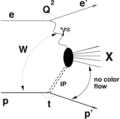
Fig. 75: Diagram representing DIS scattering on a pomeron.

In the Ingelman-Schlein approach, deep inelastic $ep$ diffractive scattering proceeds in two steps. First, a pomeron is emitted from the proton and then the virtual photon is absorbed by a constituent of the pomeron. This is depicted schematically in Fig. 75. In order to describe this process we have to introduce new variables, in addition to the ones used to describe the inclusive DIS such as $Q^{2}$, $W$, $x$ and $y$. The flux of the pomeron depends on the fraction of the proton four-momentum carried by the pomeron, $x_{{\scriptscriptstyle I\!\!P}}$, and on the square of the momentum transfer, $t$,

$$x_{{\scriptscriptstyle I\!\!P}} = \frac{q\cdot(P-P^{\prime})}{q\cdot P}\,,$$ (152)

$$t = (P-P^{\prime})^{2}\,,$$ (153)

where $P$ and $P^{\prime}$ denote the initial and final proton four-momenta respectively. If we note that by definition $M_{X}^{2}=(q+P-P^{\prime})^{2}$ and $W^{2}=(q+p)^{2}$ then it is easy to show that

$$x_{{\scriptscriptstyle I\!\!P}}=\frac{M_{X}^{2}+Q^{2}-t}{W^{2}+Q^{2}-m_{p}^{2}}\simeq\frac{M_{X}^{2}+Q^{2}}{W^{2}+Q^{2}}\,,$$ (154)

where $m_{p}$ stands for the mass of the proton and the last relation on the RHS holds for small $t$ and large $W$, a good approximation for the kinematic region of high energy diffractive scattering.

Since the deep inelastic scattering now takes place on the pomeron, we need to introduce a variable equivalent to the Bjorken $x$, but relative to the pomeron momentum. This variable is usually called $\beta$,

$$\beta=\frac{Q^{2}}{2q\cdot(P-P^{\prime})}=\frac{x}{x_{{\scriptscriptstyle I\!\!P}}}\simeq\frac{Q^{2}}{Q^{2}+M_{X}^{2}}\,,$$ (155)

where again in the last step the contribution from $t$ was neglected. Note that the definitions of the new variables are very general and do not rely on the dynamics of diffraction as assumed in the Ingelman-Schlein model.

In the same spirit one can extend the DIS cross section to include the dependence on two additional variables. It is customary to retain the variables $t$, $x_{{\scriptscriptstyle I\!\!P}}$, $x$ and $Q^{2}$. The four-fold differential cross section for $ep$ scattering can be written as

$$\frac{d^{4}\sigma^{D}}{d\,x_{{\scriptscriptstyle I\!\!P}}d\,td\,Q^{2}d\,x}=\frac{2\pi\alpha^{2}}{xQ^{4}}\left[1+(1-y)^{2}\right]F_{2}^{D(4)}(x,Q^{2},x_{{\scriptscriptstyle I\!\!P}},t)\,,$$ (156)

where for the sake of simplicity we have omitted the contribution from the longitudinal structure function. The superscript $D$ denotes the diffractive process and the number in parenthesis in the superscript of the $F_{2}^{D}$ is a reminder that the units of the structure function have changed. Keeping in mind the relation between $F_{2}$ and the absorption cross section $\sigma(\gamma^{*}p)$ we can postulate that,

$$F^{D(4)}_{2} \equiv \frac{d^{2}F_{2}^{D}(x,Q^{2},x_{{\scriptscriptstyle I\!\!P}},t)}{d\,x_{{\scriptscriptstyle I\!\!P}}d\,t}$$

$$= \frac{N}{16\pi}\beta_{a{\scriptscriptstyle I\!\!P}}^{2}(t)x_{{\scriptscriptstyle I\!\!P}}^{1-2\alpha_{{\scriptscriptstyle I\!\!P}}(t)}F_{2}^{{\scriptscriptstyle I\!\!P}}(x,Q^{2},x_{{\scriptscriptstyle I\!\!P}},t)\,.$$

If Regge factorization holds we expect that

$$F_{2}^{{\scriptscriptstyle I\!\!P}}(x,Q^{2},x_{{\scriptscriptstyle I\!\!P}},t)=F_{2}^{{\scriptscriptstyle I\!\!P}}(\frac{x}{x_{{\scriptscriptstyle I\!\!P}}},Q^{2})\,,$$ (158)

and one can think of $F_{2}^{{\scriptscriptstyle I\!\!P}}$ as the structure function of the pomeron. Because the pomeron is self-charge-conjugate and an isoscalar the density of any flavor of $\bar{q}$ is expected to be equal to the density of the corresponding $q$,

$$f_{i/{\scriptscriptstyle I\!\!P}}(x)=f_{\bar{i}/{\scriptscriptstyle I\!\!P}}(x)\,,$$ (159)

and the densities of the $u$ and $d$ quarks are also equal,

$$f_{u/{\scriptscriptstyle I\!\!P}}(x)=f_{d/{\scriptscriptstyle I\!\!P}}(x)=f_{\bar{u}/{\scriptscriptstyle I\!\!P}}(x)=f_{\bar{d}/{\scriptscriptstyle I\!\!P}}(x)\,.$$ (160)

To first approximation one can assume that there are only two parton densities in the pomeron, the quark and gluon densities. It would be tempting to assume that the strange quark density is the same as that of the $u$ and $d$ quarks. However, the $Kp$ total cross section is smaller than the $\pi p$ cross section, suggesting a possible suppression of strange quarks. As for heavier quarks, it may be assumed that their density can be dynamically generated by QCD evolution. Obviously the issue of the strange and heavy quark component of the gluon depends of the real nature of the pomeron, a subject which will be discussed in the next section.

6.3 Diffraction in QCD

Some properties of diffractive dissociation make it a very interesting study ground for QCD. Diffractive processes lead to the presence of large rapidity gaps in the final states while in QCD, in which fragmentation is driven by parton radiation, large rapidity gaps are exponentially suppressed (?). To understand diffraction in QCD one has to invoke new coherent phenomena.

In QCD the concept of the pomeron still remains mysterious. The ideas about the nature of the pomeron range from a simple diagram with two gluon exchange (?; ?) to a sophisticated gluon exchange whose properties depend on the nature of the interaction (for a review see ?). The BKFL pomeron (?; ?; ?), called sometimes hard or perturbative pomeron, would consist a ladder of (reggeized) gluons with a very special radiation pattern (strong $x$ ordering and no $k_{t}$ ordering of the gluons inside the ladder). From the theoretical point of view it becomes essential to analyze various processes in terms of which type of pomeron could be probed. The QCD picture of the pomeron points to its non-universal nature .

6.3.1 Interplay of soft and hard physics

Together with the high parton density physics of the small-$x$ regime of $ep$ scattering at HERA came the realization that the hard physics studied till now is the result of an interplay of hard and soft phenomena. In case of deep inelastic scattering the unknown soft physics is hidden in the initial parton distributions which are parameterized at a relatively small scale $Q_{0}^{2}\sim 1\,\mathrm{GeV^{2}}$. The lack of a dynamical picture of the proton structure leads to a large uncertainty about the region of phase space which has not been probed as yet. This uncertainty propagates itself in QCD predictions for high energy hard scattering at future colliders.

The ability to separate clearly the regimes dominated by soft or by hard processes is essential for exploring QCD both at a quantitative and qualitative level. A typical example of a process dominated by soft phenomena is the interaction of two large size partonic configurations such as two hadrons. A process which would lend itself to a fully perturbative calculation, and therefore hard, is the scattering of two small size heavy onium-states each consisting of a pair of heavy $q\bar{q}$ pair (?).

In deep inelastic scattering the partonic fluctuations of the virtual photon can lead to configurations of different sizes. The size of the configuration will depend on the relative transverse momentum $k_{T}$ of the $q\bar{q}$ pair. Small size configurations (large $k_{T}\sim Q/2$) are favored by phase space considerations (the phase space volume available is proportional to $k_{T}^{2}/Q^{2}$). In the QPM, in order to preserve scaling, it was necessary to suppress their presence by making them sterile. In QCD there is a simple explanation for this suppression - the effective color charge of a small size $q\bar{q}$ pair is small due to the screening of one parton by the other and therefore the interaction cross section will be small (?; ?). This phenomenon is known under the name of color transparency.

At small $x$ the smallness of the cross section is compensated by the large gluon density (see Eq. 38). The dominant mechanism for diffractive scattering of a small size $q\bar{q}$ pair is two gluon exchange and the cross section can be calculated in perturbative QCD.

For large size configurations, as noted previously, one expects to be in the regime of soft interactions, modified by the typical QCD evolution. Here the Ingelman-Schlein type model would be applicable.

This qualitative picture based on QCD considerations leads to a picture of diffraction very different from the one expected from the QPM. The origin of a large rapidity gap may be either of perturbative nature or due to soft processes. The pomeron exchange is non-universal and exhibits very different energy dependences for different initial photon configurations. Processes dominated by hard scattering are expected to have a faster energy dependence than those dominated by soft processes. The establishment of the validity of this approach has important consequences for the theoretical understanding and possible observation of unitarization effects, which is considered one of the main challenge of strong interactions.

6.3.2 Perturbative hard diffractive scattering

By perturbative hard diffractive scattering we mean a process in which the large rapidity gap is of perturbative origin. The cross section for these processes are calculable in perturbative QCD, with the parton distributions in the proton as input. For this to happen, the photon has to fluctuate into a large $k_{T}$, $q\bar{q}$ pair. Furthermore, for this process to be dominated by a two-gluon exchange, the invariant mass $M_{X}^{2}\ll Q^{2}$. By minimizing the amount of energy transferred from the proton to the virtual photon, extra radiation is suppressed. The price for forcing $M_{X}^{2}\ll Q^{2}$ is a suppression of the cross section by extra powers of $Q^{2}$.

To differentiate between diffractive processes with a hard scale but a soft component and those which can be calculated in perturbative QCD, we will call the latter perturbative diffractive scattering. Three classes of processes have been identified as possible candidates for perturbative diffractive scattering in $ep$ interactions. One class is small mass diffractive dissociation of a longitudinally polarized virtual photon, $\gamma^{*}_{L}$, which fluctuates preferentially into a small size $q\bar{q}$ configuration (?). A possible trigger for a $\gamma^{*}_{L}$ induced diffractive interaction is the production of a longitudinally polarized vector meson, such as $\rho$, $\omega$, $\phi$, $J/\psi$ or $\Upsilon$, or any of their radial excitations. Exclusive vector meson production is discussed in detail in section 7. The second class consists of diffractive, exclusive dijet production, where the invariant mass of the two jets saturates the invariant mass of the photon dissociation system (?; ?), independently of the polarization of the virtual photon. In the same category is the diffractive production of heavy flavors (?; ?). The third process is large $t$ diffractive production of vector mesons (?; ?) where $t$ is of the order of few GeV. The contribution from the soft pomeron exchange should be highly suppressed due to its steeply falling $t$ distribution. At large $t$ the proton is expected to dissociate into a multi-hadronic final state.

In perturbative diffractive processes, $d\sigma/dt|_{t=0}\sim[xG(x,Q^{2}_{\rm eff})]^{2}$, with the effective hard scale, $Q^{2}_{\rm eff}$, depending on the process. For vector meson production (?)

$$Q^{2}_{\mathrm{eff}}=Q^{2}\frac{\langle b^{2}_{L}\rangle}{\langle b^{2}_{V}\rangle}\ll Q^{2}\,,$$ (161)

where $\langle b^{2}_{L}\rangle$ and $\langle b^{2}_{V}\rangle$ are the effective sizes of the $q\bar{q}$ pair for the longitudinal photon and the vector meson respectively, while for jets with transverse momentum $p_{T}$

$$Q^{2}_{\mathrm{eff}}=\frac{p_{T}^{2}}{(1-\beta)}\geq p_{T}^{2}\,.$$ (162)

Therefore the cross section for hard diffractive processes is expected to rise with $W$ with a scale dependent power and considerably faster than for soft processes.

In QCD the slope of the pomeron trajectory, $\alpha^{\prime}_{\scriptscriptstyle I\!\!P}$, is related to the average $k_{T}$ of the partons in the exchange (?). For hard processes $k_{T}$ is expected to be large and $\alpha^{\prime}_{\scriptscriptstyle I\!\!P}\sim 1/Q^{2}$. Therefore another distinctive feature of perturbative diffractive processes is that the slope of the $t$ distribution should be universal and independent of energy (?; ?).

The interest in studying perturbative diffractive processes lies in that at very large energy (small $x$), when the density of gluons becomes very large, unitarity corrections are expected to set-in and soft phenomena will become dominant again. However because the coupling constant will remain small, it will be possible to study the approach to the unitarity limit from the perturbative regime.

6.3.3 QCD inspired models of LRG production

Only a special class of hard diffractive scattering processes lends itself to perturbative calculations. These processes are usually suppressed by extra powers of $Q^{2}$ compared to the total cross section (they are called higher twist contributions) and populate the region of large $\beta$. The experimental evidence, on the other hand, points to the presence of a large fraction of DIS events with LRG which remains relatively constant as a function of $Q^{2}$ and $W$ (?; ?) and populates evenly the $\beta$ phase space. It is thus of interest to review the phenomenological approaches which try to explain such a large fraction of diffractive-like events within QCD.

Since the first results of HERA were presented, the scientific community is burgeoning with ideas about the possible origin of hard diffraction and probable consequences. It is therefore not possible to give a complete and fair review. Instead we will present a broad classification and concentrate on discussing in more details the most popular approaches.

Regge factorization and QCD

There is a class of models which follow the original idea of Ingelman and Schlein (?). The cross section for diffractive scattering is assumed to factorize into a pomeron flux and the pomeron is assumed to consist of partons whose number densities have to be determined directly from the data, usually by applying the standard DGLAP QCD evolution.

Only recently the QCD factorization theorem was proven to hold for the leading twist diffractive structure function, $F_{2}^{D}$, of the proton measured in DIS (?), giving support to this approach. Prior to that, it was conjectured that one could introduce the concept of diffractive parton densities (?; ?) (also called differential fracture functions) and that these new parton densities would factorize similarly to the DIS parton densities and satisfy the DGLAP evolution equation (?; ?). The Regge factorization of these diffractive parton densities is an additional assumption.

A large group of physicists have explored such an approach (?; ?; ?; ?; ?; ?; ?; ?). They differ in the way one of the three major ingredients are treated: the pomeron flux, the evolution equation and the initial parton distributions. In this Ingelman-Schlein type of approach it is also natural to incorporate the exchange of sub-leading trajectories in the same way as the pomeron exchange (?; ?).

Color dipole interactions

Since in small-$x$ interactions it is rather the $q\bar{q}$ fluctuation of the photon which interacts with the target proton, it is natural to view the interaction as that of a color dipole with the proton (?; ?; ?; ?). ? have extended the dipole approach assuming that the proton also consists of color dipoles.

For diffractive scattering the dipole interacts with the proton through two-gluon exchange. The models differ in the way the two-gluon exchange is handled in QCD. Since there is no guarantee that the approach can be fully perturbative, the uncertainties are absorbed into effective parameterizations, whose parameters are derived from the inclusive DIS scattering in particular.

In these models the pomeron is non-universal and cannot be represented by a single flux. Common to this approach is the prediction of a dominant contribution of the longitudinal photon to the large $\beta$ spectrum. The small-$\beta$ spectrum is populated by a $q\bar{q}g$ configurations of the photon, while the $q\bar{q}$ configuration of the transversely polarized photon populates the mid $\beta$ region.

Perturbative QCD approach

In this approach diffractive scattering proceeds through the coupling of two-gluons to the photon (?; ?; ?; ?). For low mass diffraction the final state consists of a $q\bar{q}$ pair, while large mass diffraction includes the production of $q\bar{q}g$ final states. The dynamical content of these models differ in the treatment of QCD corrections and in the choice of the gluon density. In many respects the results are similar to the ones obtained with the dipole approach.

This approach is used to calculate high $p_{T}$ jets (?) and charm production in diffractive scattering (?; ?; ?). In the perturbative approach the charm yield is expected to be large. The only exception is the model (?) based on non-perturbative two-gluon exchange of ?.

Semi-classical approach and soft color interactions

In the semi-classical approach partonic fluctuations of the virtual photon are scattered off the proton treated as a classical color field localized within a sphere of radius $1/\Lambda$ (?). A final state color singlet partonic configuration is assumed to lead to a diffractive event while a color non-singlet configuration yields an ordinary non-diffractive event. This simple physical picture, which is a generalization of the AJM model, leads to a number of predictions (?; ?) which are independent of the details of the proton color field. In this approach the notion of pomeron does not really appear and large rapidity gaps are generated as a result of color rearrangement in the final state.

The phenomenology of the semi-classical approach is qualitatively similar to the Ingelman-Schlein approach, with a pomeron which is predominantly gluonic. The dominant partonic process is boson-gluon fusion (?) and non-perturbative soft color interactions (?) cause the formation of a color singlet final state.

6.3.4 Summary

To summarize, a tremendous theoretical progress has been achieved since the first appearance of large rapidity gaps in DIS. While the number of models may seem overwhelming, in fact in many respects they follow the same pattern and their validity is limited to specific regions. Their variety reflects the problem of the interplay of soft and hard QCD in diffraction, as well as the interplay of leading and non leading twist effects. The latter have been pretty much ignored in the region of small $x$, however they may turn out to play an important role (?; ?) and improve our understanding of the small-$x$ physics in general.

Many of the presented models have predictions which can be tested experimentally, such as Regge factorization, the $Q^{2}$ and $W$ dependence as a function of $\beta$ as well as the $t$ dependence. The characteristics of the final states is another probe for the validity of the presented ideas. The experimental program at HERA barely started and the present achievements will be summarized below.

6.4 Pre-HERA experimental results

The first evidence for the existence of a hard component in diffractive scattering was reported by the UA8 experiment (?; ?). It was based on the presence of large $p_{T}$ jets in $p\bar{p}$ interaction at $\sqrt{s}=630\,\mathrm{GeV}$ in which a proton (or anti-proton respectively) was found carrying a large fraction of the beam momentum, $0.90<x_{L}<.97$. The measurements were performed at relatively large values of $t$, $t>0.9\,\mathrm{GeV^{2}}$. Based on a sample of two jet events, the pomeron internal structure was found to be hard (?), with about $30\%$ of the sample consisting of jets carrying away all of the pomeron momentum.

6.5 Diffractive dissociation in photoproduction

Before embarking on a more detailed discussion of hard diffractive scattering at HERA, it is of interest to establish whether diffractive dissociation initiated by a real (or quasi-real) photon follows the properties observed in hadron-hadron interactions.

In fixed target experiments, diffractive dissociation of the photon was studied in $\gamma p$ interactions at centre of mass energies $\sqrt{s}\simeq 14\,\mathrm{GeV}$ (?). The double-differential cross section $d^{2}\sigma/d\,td\,M_{X}^{2}$ was measured for $M_{X}^{2}/s<0.1$ and $0.02<t<0.2\,\mathrm{GeV^{2}}$. The differential cross section was found to be dominated by the production of the $\rho$ meson. The large mass distribution was found to follow an $1/M_{X}^{2}$ dependence consistent with a large triple-pomeron presence in the diffractive amplitude. The $t$ distribution was found to be exponential with a slope $b=10.6\pm 1.0$ for $\rho$ production, while for $M_{X}^{2}>4\,\mathrm{GeV^{2}}$ the slope was found to be mass independent and roughly half of the value measured for the $\rho$. A comparison with $\pi p$ interactions with $\pi$ dissociation, performed under similar conditions showed a good agreement with Regge factorization.

Both HERA collider experiments, H1 (?) and ZEUS (?) have studied photon diffractive dissociation, using very small $Q^{2}$ (typically $Q^{2}<0.01\div 0.02\,\mathrm{GeV^{2}}$) electroproduction, in which the electron is scattered under a small angle and the interaction can be thought off as proceeding through a beam of quasi-real photons scattering of a proton target. The energy range covered by the HERA experiments is an order of magnitude larger than for the fixed target experiment. The experimental procedures used to extract the diffractive samples will be discussed in more details in the context of hard diffractive processes. Here we just report the main findings.

H1 has performed a measurement of single photon dissociation at two energies, $W=187\,\mathrm{GeV}$ and $231\,\mathrm{GeV}$. Both from the study of the energy dependence, which included the results of ?, and of the $M_{X}$ dependence, it is concluded that the triple-Regge formalism describes well the data. The extracted value of

$$\alpha_{{\scriptscriptstyle I\!\!P}}(0)=1.068\pm 0.016\pm 0.022\pm 0.041\,,$$ (163)

with the last error due to MC model uncertainties, agrees with the one from hadron-hadron interactions.

The ZEUS experiment studied the $M_{X}$ distribution at a fixed value of $W=200\,\mathrm{GeV}$ and obtained a value of

$$\alpha_{{\scriptscriptstyle I\!\!P}}(0)=1.12\pm 0.04\pm 0.08\,,$$ (164)

again in good agreement with expectations. The percentage of inelastic photon dissociation (i.e. excluding the mass region $M_{X}<m_{\phi}$) in the total cross section was found to agree with expectations of Regge factorization. In addition, the LPS detector of ZEUS was used to measure the $t$ distribution associated with photon dissociation (?). In the energy interval $176<W<225\,\mathrm{GeV}$ and for masses $4<M_{X}<32\,\mathrm{GeV}$, the $t$ distribution has an exponential behavior with

$$b=6.8\pm 0.9^{+\textstyle 1.2}_{-\textstyle 1.1}\,\mathrm{GeV^{-2}}\,.$$ (165)

It can be concluded that photon diffractive dissociation in photoproduction follows a similar pattern as single diffractive dissociation in hadron-hadron interactions.

6.6 Diffractive deep inelastic scattering at HERA

The diagram corresponding to diffractive DIS, $ep\rightarrow epX$, is presented in Fig. 75. The dissociating particle is the virtual photon emitted by the electron. The final state consists of the scattered electron and hadrons which populate the photon fragmentation region. The proton is scattered in the direction of the initial beam proton with little change in the momentum and angle.

Two major difficulties arise when studying diffractive scattering at HERA. The first difficulty is encountered in the selection of the diffractive sample. At HERA, the highly sophisticated detectors cover predominantly the photon fragmentation region, leaving out, for precise measurements, most of the proton fragmentation region. The second difficulty arises because not all events which have properties typical of diffractive dissociation are due to pomeron exchange.

In the following we first discuss the kinematic configurations of diffractive events and then the experimental procedures leading to the selection of diffractive candidate events. We then discuss the measurements of the $F_{2}^{D(3)}$ structure function ($F_{2}^{D(4)}$ integrated over $t$) and the properties of the associated final states.

6.6.1 Kinematics of diffractive final states

We first consider a typical kinematic configuration for the $\gamma^{*}p\rightarrow Xp$ reaction with mass $M_{X}$ at centre of mass energy $W$ and with $M_{X}\ll W$. For simplicity we will start by describing this configuration in the $\gamma^{*}p$ centre of mass system (cms) and assume $t=0\,\mathrm{GeV^{2}}$. The kinematics are very much like that of a two body scattering with transverse momentum $p_{T}=0$. The proton and the system $X$ move in opposite directions with longitudinal momentum $p_{L}\simeq W/2$. The respective rapidities of the proton, $y_{p}$, and of the system $X$, $y_{X}$, are

$$y_{p} = \frac{1}{2}\ln\frac{E_{p}+p_{L}}{E_{p}-p_{L}}\simeq\frac{1}{2}\ln\frac{W^{2}}{m_{p}^{2}}\,,$$ (166)

$$y_{X} = \frac{1}{2}\ln\frac{E_{X}-p_{L}}{E_{X}+p_{L}}\simeq-\frac{1}{2}\ln\frac{W^{2}}{M_{X}^{2}}\,,$$ (167)

where we have used the coordinate system of HERA with the proton moving in the positive $z$ direction and have neglected the masses compared to the energies. The rapidity separation between the proton and system $X$ is

$$\bigtriangleup y=y_{p}-y_{X}=\ln\frac{W^{2}}{m_{p}M_{X}}\,.$$ (168)

For $W=200\,\mathrm{GeV}$ and $M_{X}=20\,\mathrm{GeV}$ the rapidity separation $\bigtriangleup y\simeq 7.7$. Obviously the system $X$ will fragment into hadrons and will typically occupy a region in $\Delta y$ $\sim\ln M_{X}\simeq 3$. The proton and the fragments of system $X$ will be separated by a rapidity gap larger than 4 units. From soft hadron-hadron interactions, the typical density correlation length in rapidity is 2 units of rapidity. Therefore typical of diffractive scattering at high energy is a large rapidity gap (LRG) between the proton and the remaining hadronic system (see Fig. 76).

Fig. 76: Schematic representation of the particle distribution in the rapidity ($y$) space for a single diffractive dissociation event.

For moderate $Q^{2}$ interactions at HERA, the $\gamma^{*}p$ system is to a good approximation boosted longitudinally with respect to the laboratory system. A longitudinal boost causes all the rapidities to be shifted by the same amount and thus the basic rapidity gap structure is preserved. A proton with momentum $p_{p}=820\,\mathrm{GeV}$ has rapidity $y_{p}^{\rm lab}\simeq 7.5$. In our example the $M_{X}$ system will have $y_{X}^{\rm lab}\simeq 0$. The coverage of the main calorimeters in rapidity space is typically $-3.5<y<4$, therefore the $M_{X}$ system will be measured in the main detector, while the proton will escape detection.

Note that in events in which the proton dissociates as well, it may happen that some of the hadrons from the dissociation will be visible in the calorimeter. The presence of such events may destroy the rapidity gap between the two systems.

For calorimetric measurements of the hadronic energy flow, the pseudo-rapidity variable $\eta$ is used instead of rapidity defined as

$$\eta=-\ln\tan\frac{\theta}{2}$$ (169)

with $\theta$ the polar angle measured with respect to the proton direction. The pseudo-rapidity is a very good approximation to rapidity for particles with small mass ($E\simeq|p|$).

6.6.2 Experimental selection of diffractive samples

The selection of diffractive events in DIS proceeds in two steps. The events are first selected based on the presence of the scattered electron in the detector. The procedure follows exactly the one described for the $F_{2}$ measurements in section 4.2. For the diffractive selection three different methods have been used at HERA:

1. a reconstructed proton track was required in the leading proton spectrometer (LPS) with a fraction of the initial proton momentum $x_{L}>0.97$ (?);

2. the hadronic system $X$ measured in the central detector was required to be separated by a large rapidity gap from the rest of the hadronic final state (?; ?; ?);

3. the diffractive events were identified as the excess of events populating the small mass $M_{X}$ region, in the inclusive $\ln M_{X}^{2}$ distribution (?).

The remaining background is estimated using Monte Carlo simulation of background processes, tested on control samples. The acceptance and resolution corrections are calculated using samples of diffractive Monte Carlo simulated events tuned to reproduced the data. For the diffractive DIS analysis, the RAPGAP (?) generator, based on the Ingelman-Schlein model, is widely used. It is very similar to non-diffractive DIS generators, in which the proton is replaced by a beam of pomerons with a partonic content. Other diffractive models are used for systematic checks.

Selection based on the LPS

As in fixed target hadron-hadron interactions the cleanest selection of diffractive events with photon dissociation is based on the presence of a leading proton in the final state. By leading proton we mean a proton which carries a large fraction of the initial beam proton momentum. The spectrum of protons in a sample of DIS events has been measured in the LPS of the ZEUS experiment (?) and is shown in Fig. 77 as a function of $x_{L}=|p_{f}|/|p_{i}|$, where the subscripts $f$ and $i$ denote the final and initial protons respectively and $|p|$ stands for the absolute value of the momentum.

Fig. 77: Observed spectrum of the fraction of the proton beam momentum carried by the scattered proton, $x_{L}$. Overlaid (full line) is the result of fitting this distribution with a sum of contributions from MC generators for double dissociation (shaded area), for pion exchange (dotted line) and for photon diffractive dissociation (dashed line).

A characteristic peak is observed at $x_{L}\simeq 1$ which corresponds to photon dissociation events. The geometrical acceptance of the LPS is of the order of $10\%$. A clean sample of diffractive events is obtained by requiring $x_{L}>0.97$. Studies based on MC simulation of background processes indicate that the contamination by processes such a $\pi$ trajectory exchange or proton dissociation remains below $3\%$. The measurement of the momentum vector of the scattered proton allows to determine the $t$ value and to study the $t$ distribution in inclusive diffractive dissociation.

Selection based on large rapidity gaps

As discussed in the section on kinematic properties of diffractive photon dissociation, a large rapidity gap is expected in the hadronic final state. For inelastic DIS events, the rapidity phase space is populated evenly by final state particles.

Fig. 78: Distribution of $\eta_{\mathrm{max}}$ for DIS events. The solid circles are the data points, the dashed histogram is the result of the non-diffractive (ARIADNE) MC simulation and the full histogram is that of the DIS diffractive MC (POMPYT)

One way of establishing the presence of events with a large rapidity gap is shown in Fig. 78. Each event is assigned a variable $\eta_{\mathrm{max}}$ defined as the $\eta$ of the energy deposit in the central detector above 400 MeV closest to the proton direction. The distribution of $\eta_{\mathrm{max}}$ for DIS NC events is compared to the expectations of a DIS Monte Carlo based on the Color Dipole Model (ARIADNE (?)) for the production of the inelastic hadronic final state. A clear excess of events with large rapidity gaps is observed in the region of $\eta_{\mathrm{max}}<2$, which corresponds to an effective rapidity gap of more than 2 units of $\eta$ in the central calorimeter and possibly more than 5 units of $\eta$ relative to the initial proton. In the non-diffractive MC the LRG events are strongly suppressed in this region.

In the selection based on a rapidity gap starting in the central detector, events in which the proton has also dissociated may be erroneously assigned to single photon dissociation. This background is estimated to be $\lesssim 10\%$ for the H1 detector, for which good tagging efficiency for the hadronic final states extends into the forward region up to $\eta\simeq 7$. Only events in which the proton dissociated into a mass $M_{Y}\lesssim 1.6\,\mathrm{GeV}$ escape the tagging devices (?). In the ZEUS detector, which relies mainly on the coverage of the uranium calorimeter, masses $M_{Y}$ up to about $5.5\,\mathrm{GeV}$ remain undetected. The background is therefore larger and estimated to be $\sim 30\%$.

The requirement that the system $X$ be contained in the central detector limits the acceptance for large $x_{{\scriptscriptstyle I\!\!P}}$ values. For H1 $x_{{\scriptscriptstyle I\!\!P}}<0.05$, while for ZEUS it is $x_{{\scriptscriptstyle I\!\!P}}<0.03$. Note that for $x_{{\scriptscriptstyle I\!\!P}}>0.01$ color singlet exchanges other than the pomeron can also contribute.

Selection based on the $M_{X}$ distribution

The $M_{X}$ method to extract the diffractive contribution is based on the observation that the spectrum of the invariant mass $M_{X}$ measured in the calorimeter consists of two components with very different behavior (?). The diffractive contribution is identified as the excess of events at small $M_{X}$ above the exponential fall-off of the non-diffractive contribution with decreasing $\ln M^{2}_{X}$ (see Fig. 79). The exponential fall-off, expected in QCD (?), permits the subtraction of the non-diffractive contribution and therefore the extraction of the diffractive contribution without assuming the precise $M_{X}$ dependence of the latter.

Fig. 79: Distribution of $\ln M^{2}_{X}$ for $W$ and $Q^{2}$ as denoted in the figure. The solid line shows the exponential fall-off of the non-diffractive contribution resulting from fitting the data with Eq. (170).

The $M_{X}$ distribution is expected to be of the form

$$\frac{dN}{d\ln M_{X}^{2}}=D\;+\;c\exp(b\ln{M_{X}^{2}})\,.$$ (170)

Here, $D$ denotes the diffractive contribution. Assuming an $M_{X}^{-2}$ dependence for photon dissociation, expected to hold for $M_{X}^{2}\gg Q^{2}$ (?; ?), $D$ is a constant. The second term on the RHS represents the non-diffractive contribution. Expression (170) is fitted to the measured $\ln M_{X}^{2}$ distribution in bins of $Q^{2}$ and $W$. The fit parameters are $D$, $b$ and $c$. The fits are performed to the data in a limited range of $M_{X}^{2}$, in which the expression (170) is expected to hold to a good approximation.

The parameters of the fit are very well constrained at large $W$, where the separation of the diffractive and non-diffractive events is clearly visible. Monte Carlo studies have shown that the value of $b$ does not depend on $W$ or $Q^{2}$. The same tendency is observed in the data. As a result a single value of $b$, as determined at large $W$ and $Q^{2}$, is assumed for the fits performed in other regions.

From the results of the fitting procedure performed in each $W,~{}Q^{2}$ interval, only the parameterization of the non-diffractive background is retained. This parameterization is then extrapolated to the small $\ln M^{2}_{X}$ region and subtracted from the experimental distribution giving the diffractive contribution in the data. The results of the fit are also presented in Fig. 79.

Given the size of the background this method limits the measurements to small masses, $M_{X}<15\,\mathrm{GeV}$ and $x_{{\scriptscriptstyle I\!\!P}}\lesssim 0.01$, dominated by pomeron exchange. The background from events in which the proton also dissociated remains the same as for the LRG method.

6.6.3 Measurements of $F_{2}^{D}$

The measurements of $F_{2}^{D(3)}$ have been performed by H1 and ZEUS. The early results (?; ?) were compatible with Regge factorization. However, the values of $\alpha_{{\scriptscriptstyle I\!\!P}}$ determined from the $x_{{\scriptscriptstyle I\!\!P}}$ dependence for fixed values of $Q^{2}$ and $\beta$ were inconclusive as to the nature of the pomeron probed in DIS. The lack of $Q^{2}$ dependence established that in diffractive scattering the virtual photon was scattering off a point-like particle.

Fig. 80: The diffractive structure function $F_{2}^{D(3)}\,(\beta,\,Q^{2},\,x_{{\scriptscriptstyle I\!\!P}})$ multiplied by $x_{{\scriptscriptstyle I\!\!P}}$ as a function of $x_{{\scriptscriptstyle I\!\!P}}$ (solid points) for fixed values of $\beta$ and $Q^{2}$ as denoted in the figure. The solid line is the result of a Regge fit in which the pomeron and the reggeon exchange contribute with maximum interference. Also shown is the pomeron contribution alone (dashed line) and including the interference (dotted line).

The recent measurements of $F_{2}^{D(3)}$ by the H1 experiment (?) are based on a ten-fold increase in statistics (integrated luminosity of $1.96\,\mathrm{pb^{-1}}$) and cover the kinematic region, $4.5<Q^{2}<75\,\mathrm{GeV^{2}}$, $2\cdot 10^{-4}<x_{{\scriptscriptstyle I\!\!P}}<0.04$ and $0.04<\beta<0.9$. The analysis requires the presence in the event of a large rapidity gap, of at least 4 units in rapidity. The hadronic final state is required to be contained in the main calorimeter which provides, together with the tracking detectors, the measurement of the invariant mass $M_{X}$. The results of these measurements are shown in Fig. 80, where the values of $x_{{\scriptscriptstyle I\!\!P}}F_{2}^{D(3)}\,(\beta,\,Q^{2},\,x_{{\scriptscriptstyle I\!\!P}})$ are displayed as a function of $x_{{\scriptscriptstyle I\!\!P}}$ for different values of $\beta$ and $Q^{2}$. The $x_{{\scriptscriptstyle I\!\!P}}$ dependence of $F_{2}^{D(3)}$ is seen to change with $\beta$ and remains fairly independent of $Q^{2}$.

Fig. 81: The diffractive structure function of $F_{2}^{D(4)}\,(\beta,\,Q^{2},\,x_{{\scriptscriptstyle I\!\!P}},\,t)$ multiplied by $x_{{\scriptscriptstyle I\!\!P}}$ as a function of $x_{{\scriptscriptstyle I\!\!P}}$ (solid points) for fixed values of $\beta$ as denoted in the figure, $Q^{2}=8\,\mathrm{GeV^{2}}$ and $|t|=0.17\,\mathrm{GeV^{2}}$. Also shown is the result of the fit assuming an $(1/x_{{\scriptscriptstyle I\!\!P}})^{a}$ dependence, independent of $\beta$.

The ZEUS experiment has used a sample of LPS tagged DIS events to measure $F_{2}^{D(4)}$ in the range $5<Q^{2}<20\,\mathrm{GeV^{2}}$, $x_{L}>0.97$, $0.015<\beta<0.5$ and $0.073<|t|<0.4\,\mathrm{GeV^{-2}}$. The sample corresponds to an integrated luminosity of $900\,\mathrm{nb^{-1}}$. The results of the measurement at $Q^{2}=8\,\mathrm{GeV^{2}}$ and $|t|=0.17\,\mathrm{GeV^{-2}}$ are displayed in Fig. 81. The measurement are confined to relatively large values of $x_{{\scriptscriptstyle I\!\!P}}$ especially at small $\beta$. The data are compatible with Regge factorization, albeit the significance is limited by the dominant statistical error. The same data sample was used to determine the $t$ distribution, which was found to follow an exponential behavior as seen in Fig. 82.

Fig. 82: The differential cross section $d\!\sigma/d\!t$ for diffractive DIS events with a leading proton of $x_{L}>0.97$, in the range $5<Q^{2}<20\,\mathrm{GeV^{2}}$, $50<W<270\,\mathrm{GeV}$ and $0.015<\beta<0.5$. The line is the result of an exponential fit.

For the 1994 DIS data, corresponding to an integrated luminosity of $2.61\,\mathrm{pb^{-1}}$, the ZEUS experiment has used the $M_{X}$ method to determine the $W$ and $Q^{2}$ dependence of the $\gamma^{*}p$ photon diffractive dissociation cross section (?). The measurements were performed for small masses, $M_{X}<15\,\mathrm{GeV}$, and cover the range $7<Q^{2}<140\,\mathrm{GeV^{2}}$ and $60<W<200\,\mathrm{GeV}$. The results are displayed in Fig. 83. The differential cross section $d\sigma/dM_{X}$ is shown as a function of $W$ in bins of $Q^{2}$ and $M_{X}$. The contribution of the photon dissociation accompanied by small mass proton dissociation has not been subtracted. A strong increase with $W$ is observed for masses $M_{X}<7.5\,\mathrm{GeV}$.

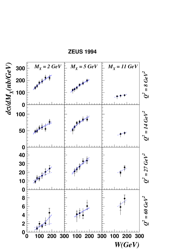
Fig. 83: The differential cross section $d\!\sigma/d\!M_{X}$ as a function of the $\gamma^{*}p$ center-of-mass of mass energy $W$ for fixed values of $Q^{2}$ and for ranges of $M_{X}$ as denoted in the figure. The solid line is the result of a fit with the function $d\!\sigma/d\!M_{X}\propto W^{a}$ in each of the bins separately. The dashed line is the result of the fit with $a$ the same for all bins.

The corresponding $F_{2}^{D(3)}$ shows a reasonable agreement with the H1 measurements (?) and the LPS measurements in the overlap region.

The $x_{{\scriptscriptstyle I\!\!P}}$ and $W$ dependence

In the simple Regge model in which $F_{2}^{D(3)}$ factorises into

$$F_{2}^{D(3)}=f_{{\scriptscriptstyle I\!\!P}/p}(x_{{\scriptscriptstyle I\!\!P}})F_{2}^{{\scriptscriptstyle I\!\!P}}\,(\beta,\,Q^{2})\,,$$ (171)

the $x_{{\scriptscriptstyle I\!\!P}}$ dependence is expected to follow a $x_{{\scriptscriptstyle I\!\!P}}^{-n}$ dependence, where $n=2\bar{\alpha}_{\scriptscriptstyle I\!\!P}-1$, independently of $\beta$ and $Q^{2}$. Here $\bar{\alpha}_{\scriptscriptstyle I\!\!P}$ stands for a value of $\alpha_{{\scriptscriptstyle I\!\!P}}(t)$ averaged over the $t$ distribution. The value of $n$ can be also obtained from the $W$ dependence of the $\gamma^{*}p$ cross section for fixed $Q^{2}$ and $M_{X}$,

$$\sigma^{D}(\gamma^{*}p)\sim Q^{2}F_{2}^{D}\sim Q^{2}x_{{\scriptscriptstyle I\!\!P}}^{-n}\sim Q^{2}\left(\frac{W^{2}+Q^{2}}{M_{X}^{2}+Q^{2}}\right)^{n}\sim W^{2n}\,,$$ (172)

where in the last step the approximation $Q^{2}\ll W^{2}$ is made.

A fit to the H1 data (?) with a single power $n$ yields a poor $\chi^{2}$. The exchange of a single factorisable Regge trajectory in the $t$ channel does not provide an acceptable description. However if one assumes in addition to the pomeron exchange the contribution of a sub-leading reggeon trajectory, the quality of the fit improves tremendously. In the fit the intercept of the pomeron $\alpha_{{\scriptscriptstyle I\!\!P}}(0)$ and of the reggeon $\alpha_{{\scriptscriptstyle I\!\!R}}(0)$ are kept as free parameters, as well as their relative contribution. The results are,

$$\alpha_{{\scriptscriptstyle I\!\!P}}(0) = 1.203\pm 0.020\pm 0.013^{+\textstyle 0.030}_{-\textstyle 0.035}\,,$$ (173)

$$\alpha_{{\scriptscriptstyle I\!\!R}}(0) = 0.50\pm 0.11\pm 0.11^{+\textstyle 0.09}_{-\textstyle 0.10}\,,$$ (174)

where the last error depends on the details of how the two contributions are added. The results of one of the models, in which a maximal interference between the pomeron and reggeon exchange is assumed, is presented in Fig. 80.

The value of $\alpha_{{\scriptscriptstyle I\!\!R}}(0)$ agrees with the value of $\simeq 0.55$ obtained in an analysis of total hadronic cross sections (?). The value of $\alpha_{{\scriptscriptstyle I\!\!P}}(0)$ is significantly larger than expected for the soft pomeron (?; ?).

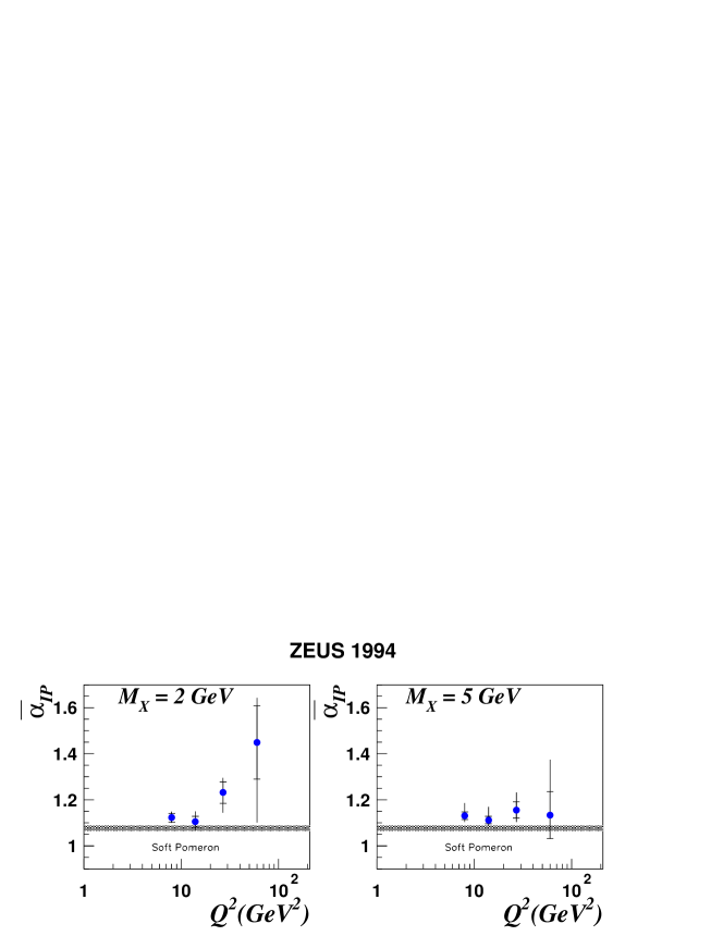
Fig. 84: The value of $\bar{\alpha}_{\scriptscriptstyle I\!\!P}$ as a function of $Q^{2}$ and for two mass ranges $M_{X}$ as derived from the fit to the $W$ dependence of the cross section. Also shown are the result expected for the soft pomeron exchange (?) assuming $\alpha^{\prime}_{\scriptscriptstyle I\!\!P}=0.25\,\mathrm{GeV^{-2}}$.

In the ZEUS data, $\alpha_{{\scriptscriptstyle I\!\!P}}(0)$ is derived from fits to the $W$ dependence of the $\gamma^{*}p$ cross section, assumed to have the form $W^{a}$, at each value of $Q^{2}$ and mass $M_{X}$ (?). The value of $a$ is related to $\alpha_{{\scriptscriptstyle I\!\!P}}(0)$ through the relation

$$a=4\left(\alpha_{{\scriptscriptstyle I\!\!P}}(0)-1-[0.03]\right)\,,$$

where the term in brackets is a correction due to averaging over the $t$ distribution, assuming $\alpha_{{\scriptscriptstyle I\!\!P}}^{\prime}=0.25\,\mathrm{GeV^{-2}}$ and $b=7\,\mathrm{GeV^{-2}}$. The fitted curves are displayed in Fig. 83 while the results of the fit for $\alpha_{{\scriptscriptstyle I\!\!P}}$ are presented in Fig. 84 as a function of $Q^{2}$ for two ranges of masses. For all values of $Q^{2}$ and $M_{X}$ the value of $\alpha_{{\scriptscriptstyle I\!\!P}}$ lies above the highest expectations from soft Regge phenomenology (?). Given the large systematic errors at large $Q^{2}$ it is not possible to draw conclusions on any possible $Q^{2}$ dependence. The value of $\alpha_{{\scriptscriptstyle I\!\!P}}$ averaged over the whole measured kinematic range is,

$$\alpha_{{\scriptscriptstyle I\!\!P}}(0)=1.16\pm 0.01^{+\textstyle 0.04}_{-\textstyle 0.01}\,,$$ (175)

compatible within errors with the value obtained in the H1 analysis. No correction for contribution of sub-leading trajectories was attempted as the measurements correspond to $x_{{\scriptscriptstyle I\!\!P}}\lesssim 0.01$ in which the pomeron exchange is dominant. The presence of sub-leading reggeon contributions may however explain the relative flatness of the $x_{{\scriptscriptstyle I\!\!P}}F_{2}^{D(4)}$ distribution measured with the LPS tag at larger $x_{{\scriptscriptstyle I\!\!P}}$ values (see Fig. 81).

Fig. 85: Ratio of the diffractive cross section $\sigma^{\rm diff}$, integrated over the mass range indicated in the figure, to the total DIS cross section $\sigma_{\rm tot}$ as a function of $W$ for different values of $Q^{2}$.

The $W$ dependence of the diffractive cross section as measured in ZEUS had been compared to the $W$ dependence of the total $\gamma^{*}p$ cross section $\sigma_{\rm tot}$. The latter was derived from a parameterization of the measured $F_{2}$ of the proton. The ratio $r_{D}$ defined as

$$r_{D}=\frac{1}{\sigma_{\rm tot}(\gamma^{*}p)}\int_{M_{X}\mathrm{bin}}\frac{d\sigma_{D}(\gamma^{*}p)}{d\!M_{X}}d\!M_{X}\,,$$ (176)

is plotted in Fig. 85 as a function of $W$. It is interesting to note that the ratio is within errors constant with $W$. This is unlike hadron-hadron interactions for which this ratio decreases strongly with $W$ (?).

The $Q^{2}$ dependence

Fig. 86: The structure function $x_{{\scriptscriptstyle I\!\!P}}F_{2}^{D(3)}$ as a function of $Q^{2}$ for $x_{{\scriptscriptstyle I\!\!P}}=0.003$ and for different values of $\beta$ as denoted in the figure. The solid line is the result of the QCD fit which includes the evolution of the pomeron and reggeon contributions. The dashed line represents the pomeron contribution only. Figures (a) and (b) differ in the assumptions about parton distributions in the pomeron at $Q^{2}_{0}=3\,\mathrm{GeV^{2}}$ as described in the figure.

The $Q^{2}$ dependence of $x_{{\scriptscriptstyle I\!\!P}}F_{2}^{D(3)}$ has been determined by H1 for $x_{{\scriptscriptstyle I\!\!P}}=0.003$ and is shown in Fig. 86 for a range of $\beta$ values. Scaling violation is observed for $\beta\leq 0.4$ where $F_{2}^{D(3)}$ increases with $Q^{2}$. For larger $\beta$ values the $Q^{2}$ dependence is mild with a tendency of $F_{2}^{D(3)}$ to decrease with increasing $Q^{2}$. The pattern of scaling violation is different from the one observed for the inclusive $F_{2}$ of the proton, especially at larger values of $\beta$. The slow decrease with $Q^{2}$ interpreted in terms of QCD evolution signals a substantial presence of gluons at large $\beta$. The radiation of quarks by gluons compensates the migration of quarks radiated by quarks towards lower values of $\beta$.

The $Q^{2}$ dependence of $r_{D}$ at low mass is much stronger (see Fig. 85) than at larger masses where it almost disappears, indicating that the diffractive production of a fixed low mass is suppressed roughly by an extra power of $Q^{2}$ relative to the total cross section. This is not necessarily in variance with the milder logarithmic dependence observed in the $H1$ data as it may reflect the large $\beta$ dependence of $F_{2}^{D(3)}$. For a fixed $M_{X}$ the increase of $Q^{2}$ corresponds to an increase in $\beta$. The $Q^{2}$ dependence observed here is not unlike the one observed in exclusive vector meson production.

The $\beta$ dependence

Fig. 87: The structure function $x_{{\scriptscriptstyle I\!\!P}}F_{2}^{D(3)}$ as a function of $\beta$ for $x_{{\scriptscriptstyle I\!\!P}}=0.003$ and for different values of $Q^{2}$ as denoted in the figure. The solid line is the result of the QCD fit which includes the evolution of the pomeron and reggeon contributions. The dashed line represents the pomeron contribution only. Figures (a) and (b) differ in the assumptions about parton distributions in the pomeron at $Q^{2}_{0}=3\,\mathrm{GeV^{2}}$ as described in the figure.

The $\beta$ dependence of $x_{{\scriptscriptstyle I\!\!P}}F_{2}^{D(3)}$ as determined by H1 for $x_{{\scriptscriptstyle I\!\!P}}=0.003$ is shown in Fig. 87 for different $Q^{2}$ values. The $\beta$ dependence is relatively flat at small $Q^{2}$ and increases towards lower $\beta$ as $Q^{2}$ increases. The same effect is observed by the ZEUS experiment.

The $t$ dependence

The $t$ distribution measured by ZEUS (see Fig. 82) has been fitted with a single exponential function yielding a value of the slope $b$,

$$b=7.2\pm 1.1^{+\textstyle 0.7}_{-\textstyle 0.9}\,\mathrm{GeV^{-2}}\,.$$ (177)

It is interesting to note that the slope of the $t$ distribution at an average $Q^{2}=8\,\mathrm{GeV^{2}}$ is larger than the slope of the $t$ distribution measured in this experiment for exclusive $J/\psi$ photoproduction (?) ($b=4.6\pm 0.6~{}\,\mathrm{GeV^{-2}}$). This may be an indication that in the mass range covered by the LPS ($0.015<\beta<0.5$)), soft processes contribute to virtual photon dissociation.

Comparison with Models

Fig. 88: The structure function $x_{{\scriptscriptstyle I\!\!P}}F_{2}^{D(3)}$ as a function of $x_{{\scriptscriptstyle I\!\!P}}$, obtained by ZEUS with the $M_{X}$ method (solid points) compared to expectations of QCD motivated models: BEKW (?), NZ (?), BP (?). Note that the BP curve includes the contribution of the reggeon trajectory as determined by the H1 experiment (?).

The ZEUS measurements of $F_{2}^{D(3)}$ have been compared to the predictions of a selected number of models representative of the present theoretical ideas behind inclusive DIS diffractive scattering:

1. the model of ?;

2. the model of ?;

3. the model of ?;

The predictions are shown in Fig. 88.

In the semi-classical approach to diffractive DIS (?), for which there are no numerical predictions as yet, it is expected that the $W$ dependence of diffractive dissociation will be similar to that of the inclusive DIS, a feature which is borne in the data.

6.6.4 Final states in diffractive DIS

The topological structure of the hadronic final states emerging from the diffractive dissociation of virtual photons should reflect the underlying production mechanism. It is convenient here to use the language of photon partonic fluctuations. For diffractive scattering dominated by the AJM configurations, one would expect the final state in the $\gamma^{*}I\!\!P$ centre of mass system to consists of two jets of particles aligned along the $\gamma^{*}I\!\!P$ collision axis. The small size configurations would materialize as two jets aligned along an axis rotated relative to the $\gamma^{*}I\!\!P$ collision axis to reflect the large $k_{T}$ of the quarks relative to the photon. Here an analogy with the final states observed in $e^{+}e^{-}$ annihilation into two quarks can be drawn. In models in which the pomeron is viewed as consisting of quarks and gluons, large $k_{T}$ jets in the $\gamma^{*}I\!\!P$ system would be accompanied by the ”remnant of the pomeron”.

Fig. 89: Diagrams representing possible partonic configurations of the photon dissociation in DIS. From left to right, the Born term, QCD Compton process and boson-gluon fusion process.

Possible configurations of the final state are shown diagrammatically in Fig. 89. In each configuration some $k_{T}$ can be assigned to the partons, in particular for the QCD Compton and boson-gluon fusion diagram. However, even the initial partons in the pomeron could have large $k_{T}$.

The relatively small invariant mass $M_{X}$ of the dissociative system makes a jet-search analysis of the final states very inefficient. Topological studies can be carried out by invoking event shape variables. These variables were very successful in describing the partonic nature of the hadronic final states in $e^{+}e^{-}$ scattering at centre of mass energies which were too low to resolve three-jet from two-jet events (?) and which correspond to the typical values of $M_{X}$ considered here.

Charm production is also believed to be a sensitive probe for the mechanism underlying diffractive hard scattering (?). The mass of the charm quark provides the hard scale for the perturbative approach to be applicable.

Event shape variables

The momentum tensor for a state $X$, consisting of $N$ particles with momentum vectors $\vec{p}_{i}$ in the rest frame of system $X$, is defined as

$$Z_{m,n}=\sum_{i=1}^{N}p_{im}p_{in}\,,$$ (178)

where the subscripts $m$ and $n$ denote the three coordinates of vector $\vec{p}$ (?). The diagonalization of $Z_{mn}$ yields three axes $\vec{n}_{k}$ and three eigenvalues $\lambda_{k}=\sum_{i=1}^{N}(\vec{p}_{i}\cdot\vec{n}_{k})^{2}$. The normalized eigenvalues $\Lambda_{k}=\lambda_{k}/\sum_{i=1}^{N}(\vec{p}_{i})^{2}$ can be ordered in such a way that $\Lambda_{1}<\Lambda_{2}<\Lambda_{3}$. The corresponding unit vectors $\vec{n}_{i}$ define a reference frame in which vector $\vec{n}_{3}$ is the unit vector along the principal axis, the so called sphericity axis, which minimizes the sum of the squared transverse momenta. The event plane is defined by $\vec{n}_{2}$ and $\vec{n}_{3}$, while $\vec{n}_{1}$ defines the direction perpendicular to the event plane. Sphericity $S$ is defined as

$$S=\frac{3}{2}(\Lambda_{1}+\Lambda_{2})=\frac{3}{2}\min_{\vec{n}}\frac{\sum_{i=1}^{n}p_{T_{i}}^{2}}{\sum_{i=1}^{n}p_{i}^{2}}\;\;\;\;\;\;\;\;(\vec{n}=\vec{n}_{3}).$$ (179)

Sphericity indicates the total $p_{T}^{2}$ with respect to the event axis. For isotropic distributions of particles in the phase space $S=1$. In models with a constant limited transverse momentum of particles relative to the interaction axis, the mean sphericity values are inversely proportional to the centre of mass energy. For pencil like two-jet events $S=0$. For collimated jets, the polar angle $\theta_{S}$ of the sphericity axis with respect to the $\gamma^{*}I\!\!P$ axis is a measure of the alignment of the jets with respect to the interaction axis.

Alternatively one can use the thrust variable $T$ (?; ?). The thrust axis, denoted by the unit vector $\vec{n}_{T}$, is the direction in space which maximizes the longitudinal momentum of particles. Thrust is then defined as

$$T=\max_{\vec{n}}\frac{\sum_{i=1}^{n}|\vec{p}_{i}\cdot\vec{n}|}{\sum_{i=1}^{n}|\vec{p}_{i}|}\;\;\;\;\;\;\;\;(\vec{n}=\vec{n}_{T}).$$ (180)

Isotropic events are characterized by $T\simeq 0.5$, while for collimated two-jet events $T\simeq 1$. For a symmetric three particle configuration $T=2/3$ and the thrust axis is arbitrary, while for an asymmetric topology the thrust axis is pointing in the direction of the most energetic particle and $T>2/3$.

Fig. 90: Values of thrust and sphericity expected for different configurations of hadrons in the final state.

Once the thrust axis is found, the hadrons can be clustered into two jets, based on the sign of their longitudinal momentum projected onto $\vec{n}_{T}$. By definition the two jets will have equal in size and opposite in direction momentum-vectors. One can then defined the thrust jet transverse momentum $P_{T}$, as the transverse momentum of one of the jets relative to the $\gamma^{*}I\!\!P$ axis. For large values of $P_{T}$ the value of $T$ will differentiate between two partons with large $k_{T}$ and a three parton configuration.

The values of $T$ and $S$ expected for three selected configurations of hadrons are summarized in Fig. 90.

Event shapes in LRG events

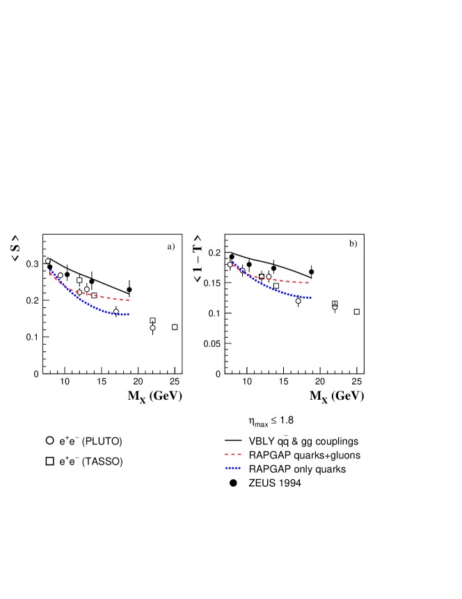
Fig. 91: The mean sphericity, $\langle S\rangle$, a) and one minus mean thrust, $\langle 1-T\rangle$, b) as a function of the mass $M_{X}$. The ZEUS data (solid dots) selected with an $\eta_{\mathrm{max}}<1.8$ cut cover the kinematic range $5\leq Q^{2}\leq 185\,\mathrm{GeV^{2}}$ and $160\leq W\leq 250\,\mathrm{GeV}$. Also shown are data from $e^{+}e^{-}$ annihilation (?; ?). The lines represent the expectations of various MC models in the kinematic range of the ZEUS data.

Fig. 92: The mean thrust as a function of the inverse mass $1/M_{X}$ for a) DIS events selected with a large rapidity gap in the region $10<Q^{2}<100\,\mathrm{GeV}2$, $x_{{\scriptscriptstyle I\!\!P}}<0.05$ (solid point) and $e^{+}e^{-}$ annihilation data (?; ?; ?; ?; ?; ?) (empty squares). In b), the data are compared with expectations of the RAPGAP MC model (RG ME+PS) for two samples od DIS events with different thrust transverse momentum $P_{T}$.

Both HERA experiments have studied the event shapes in the DIS photon diffractive dissociation (?; ?). The studies of the ZEUS experiment (?) in the region of $5\leq Q^{2}\leq 185\,\mathrm{GeV^{2}}$ are confined to a sample of events selected with requirements of $\eta_{\mathrm{max}}\leq 1.8$ and $7\leq M_{X}\leq 25\,\mathrm{GeV}$. To increase the acceptance of diffractive events selected with these cuts the $W$ range is further restricted to $160\leq W\leq 250\,\mathrm{GeV}$. The selection of H1 follows that for the $F_{2}^{D(3)}$ analysis, where the system $X$ is contained within the central calorimeter and a large rapidity gap of about 4 units in the forward region is required. The analysis is performed for $10<Q^{2}<100\,\mathrm{GeV^{2}}$, $x_{{\scriptscriptstyle I\!\!P}}<0.05$ and $4<M_{X}<36\,\mathrm{GeV}$.

Both experiments observe that as the mass $M_{X}$ increases the hadronic final state is more and more collimated along the thrust or sphericity axis. This is shown in Fig. 91a,b for the ZEUS data and in Fig. 92a for the H1 data. The sphericity is seen to decrease, while the thrust is increasing with increasing $M_{X}$. This is a sign of jet formation along the respective axes. The level of collimation is compared to the one measured in $e^{+}e^{-}$ experiments, which is representative of a final state consisting of a $q\bar{q}$ pair with possible extra gluon radiation. Both experiments observe that the jets in diffractive events are less collimated than in $e^{+}e^{-}$ interactions indicating that $q\bar{q}$ configurations alone cannot explain the observed features and higher parton multiplicity are required. This conclusion is supported by the comparison of data with the RAPGAP MC model with final states consisting of only $q\bar{q}$ pairs which does not give a good representation of the data.

Fig. 93: Fraction of events with thrust transverse momentum $P_{T}^{2}>3\,\mathrm{GeV^{2}}$ as a function of $M_{X}$ (data points), compared to the predictions of various MC models which differ in the treatment of the origin of the large rapidity gaps (RG - RAPGAP, factorizable partonic pomeron; LEPTO - soft color interactions) and in the final state fragmentation. ME+PS stands for matrix elements with parton showers for higher order corrections, while AR+CD stands for the ARIADNE color dipole model.

The data were also compared to the expectations of the RAPGAP MC in which both the quark and the gluon component of the pomeron, as well as all the diagrams of Fig. 89, are included in the generation of final states (see Fig. 91a,b and 92b). The MC samples used by the two experiments differ in the description of the partonic content of the pomeron and in the fragmentation of the final states. The version used by the H1 experiment, which was tuned to reproduced best the cross section measurements and the characteristics of the hadronic final states, describes the $1/M_{X}$ dependence of $T$ very well. However even in this version of the RAPGAP model, the tail of the large $P_{T}^{2}$ is not properly reproduced as can be seen in Fig. 93.

The ZEUS data have been compared to the VBLY model (?) which differs from the RAPGAP model in that the partons, quarks and gluons, which couple to the photon, acquire a substantial $k_{T}$ as their distribution is obtained assuming a point-like coupling to a scalar particle. This leads effectively to larger $P_{T}$ values. In the particular region of phase space selected in the ZEUS experiment, the VBLY model gives a better description of the ZEUS data than the RAPGAP model.

Note that the $\eta_{\mathrm{max}}$ cut applied to select the diffractive sample in the ZEUS experiment was not corrected for, as the correction was found to be strongly model dependent (?). For larger masses, this cut may bias the hadronic configurations towards those which have been produced with a large transverse momentum relative to the $\gamma^{*}p$ axis. It may well be that the excess of events with large $P_{T}$ over the RAPGAP expectations observed in the H1 sample and the disagreement of the ZEUS data with RAPGAP have a common origin.

In conclusion the features observed in the study of event shape variables cannot be explained by a pure $q\bar{q}$ configuration, even assuming a large relative $k_{T}$ of the pair. A substantial contribution of $q\bar{q}g$ or higher partonic multiplicities is required in the final states.

Charm production

The experimental signature for charm production is a particular decay channel of the $D^{*\pm}$ mesons. The $D^{*}$ mesons are reconstructed from their decay products through the chain $D^{*}\!\rightarrow D^{0}\pi_{s}^{+}\!(K^{-}\pi^{+})\pi_{s}^{+}$ (and the charge conjugate), where the subscript $s$ stands for the slower pion of the pair. The small mass difference $M(D^{*})-M(D^{0})=145.42\pm 0.05\,\mathrm{MeV}$ yields a prominent signal just above the threshold of the $\Delta M=M(K\pi\pi_{s})-M(K\pi)$ distribution, where the phase space contribution is highly suppressed.

Fig. 94: Distribution of the mass difference between the $D^{*}$ and $D^{0}$ candidates, $\Delta M=M(D^{*})-M(D^{0})$, for the diffractive DIS sample selected with $\eta_{\mathrm{max}}<1.5$, $x_{{\scriptscriptstyle I\!\!P}}<0.012$ and $\beta<0.8$. The solid dots indicate the signal distribution, while the dashed histogram represents the background distribution from wrong charge combinations. The solid line is the result of fitting a Gaussian distribution and a threshold function of the form $a(\Delta M-m_{pi})^{b}$.

Charm production associated with large rapidity gaps has been searched for both in deep inelastic scattering (?; ?) and in hard photoproduction (?). The $\Delta M$ distribution for events with a large rapidity gap is shown in Fig. 94 for deep inelastic scattering with $Q^{2}>3\,\mathrm{GeV^{2}}$. The charm production cross section, integrated over the phase space of the measurements are compatible with expectations based on the RAPGAP MC model with gluons as obtained from the $F_{2}^{D(3)}$ measurements. In deep inelastic scattering (?), for $3<Q^{2}<150\,\mathrm{GeV^{2}}$, $0.02<y<0.7$, $p_{T}(D^{*})>1.5\,\mathrm{GeV}$ and $|\eta^{D*}|<1.5$, the fraction of diffractively produced events with $.002<x_{{\scriptscriptstyle I\!\!P}}<0.012$ was found to be $7\pm 2.2\%$ of the total $D^{*}$ sample.

The available charm production studies suffer from large statistical errors. However, the present results point to a substantial charm production in hard diffractive processes and give a strong support to models in which diffractive production is mediated through gluons.

6.7 Hard diffraction in photoproduction

In hadron-hadron interactions two processes have been proposed to study the nature of the pomeron. Both involve the production of large $p_{T}$ jets as a trigger for the partonic nature of the interaction. One process is the production of jets embedded in a hadronic final state well separated in rapidity from the target hadron, originally proposed by Ingelman and Schlein (?) and the other is the production of two large $p_{T}$ jets separated by a large rapidity gap proposed by Bjorken (?). These two types of diffractive processes may in principle be very different in nature. In the first process, in which the hadron identity is to be preserved, the momentum transfer square $t$ is small, while in the second process, $t$ is large and the diffractive exchange takes place between two partons.

Both processes can be studied at HERA in the interactions of quasi-real photons with protons. The photon is known to display a partonic structure in the presence of strong interactions (see section 5.2.1). Two components can be identified in the structure of the photon, the large size partonic configuration where the photon behaves essentially as a vector meson state and the small size configuration, called the anomalous contribution. The presence of the latter makes the photon interactions different from that of hadrons and is at the origin of the so called direct photon contribution to hard processes. In the spirit of QCD color transparency phenomena, in which final states interactions are suppressed for the interactions of small size configurations, the LRG production could be enhanced in hard photoproduction processes.

6.7.1 Diffractive jet production in photoproduction

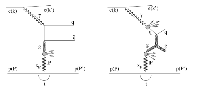
Fig. 95: Examples of diagrams contributing to dijet production in hard diffractive photoproduction. Left – direct photon contribution, right – resolved photon contribution.

In the Ingelman-Schlein model of hard diffractive scattering the pomeron exchange also contributes to the production of large $p_{T}$ jets associated with a photon dissociation system. Examples of diagrams for diffractive dijet production, one for a direct and one of a resolved process, are shown in Fig. 95. The quark content of the pomeron can be measured in DIS, while jet production in photoproduction is sensitive to both the quark and gluon content of the interacting particles.

Theoretical background

The cross section for dijet production can be expressed through universal parton distributions if use is made of the QCD factorization theorem (see section 5.2.1). For the diffractive dijet production,

$$ep\rightarrow ep+{\rm jet}_{1}+{\rm jet}_{2}+X^{\prime}\,,$$ (181)

where $X^{\prime}$ denotes the rest of the final state not associated with jets, the cross section can be symbolically written as

$$\sigma(y,x_{{\scriptscriptstyle I\!\!P}},t:p_{T}^{2},\hat{s})=$$

$$f_{\gamma/e}(y)f_{{\scriptscriptstyle I\!\!P}/p}(x_{{\scriptscriptstyle I\!\!P}},t)\sum_{i,j}\sum_{k,l}f_{i/\gamma}(x_{\gamma},p_{T}^{2})f_{j/{\scriptscriptstyle I\!\!P}}(\beta,p_{T}^{2})\hat{\sigma}_{i+j\rightarrow k+l}(p_{T}^{2},\hat{s})\,,$$

where $f$ denotes the respective fluxes and Regge factorization is assumed for the pomeron flux. The first sum runs over all possible types of partons present in the photon and the pomeron and the second sum runs over all possible types of final state partons. The cross section $\hat{\sigma}(p_{T}^{2},\hat{s})$ for two body collisions, $i+j\rightarrow k+l$, depends on the centre of mass energy, $\hat{s}=x_{{\scriptscriptstyle I\!\!P}}\beta x_{\gamma}W$, and the transverse momentum of the outgoing partons, $p_{T}$. For large values of $p_{T}$ the cross section can be reliably calculated in perturbative QCD.

The QCD factorization theorem has been proven to hold for diffractive DIS but fails for hard diffractive processes in hadron-hadron collisions (?). This would imply that expression (6.7.1) is expected to hold for direct photon processes (i.e. $f_{i/\gamma}(x_{\gamma},p_{T}^{2})=\delta(1-x_{\gamma})$) but not for resolved photon processes.

The interest of studying jet production in diffractive photoproduction in combination with the DIS measurements allows to address the issues of the gluon content of the pomeron, the validity of QCD factorization and the validity of Regge factorization.

HERA data

Fig. 96: Distribution of $\eta_{\mathrm{max}}$ in tagged $\gamma p$ interactions containing jets with transverse energy $E_{T}>5\,\mathrm{GeV}$ in the interval $-1.5<\eta_{jet}<2.5$ (dots). The solid line shows MC expectations for a mixture of diffractive and non-diffractive processes. The dashed line denotes the non-diffractive contribution from the MC model (PYTHIA (?)).

The search for jet production associated with a large rapidity gap in the proton fragmentation region  (?; ?) has established the presence of hard diffractive scattering in photoproduction. An example of the $\eta_{\mathrm{max}}$ distribution for the inclusive sample of photoproduction events with a reconstructed jet with $E_{T}>4\,\mathrm{GeV}$ is shown in Fig. 96. An excess of events at small $\eta_{\mathrm{max}}$ over the expectations for non-diffractive jet production is observed. The shape of the $\eta_{\mathrm{max}}$ distribution can be well reproduced if the non-diffractive model is supplemented with hard diffractive processes assuming a pomeron consisting of hard gluons. The Ingelman-Schlein model is implemented in the POMPYT MC generator (?).

To describe the measured inclusive diffractive jet production cross section within the Ingelman-Schlein model a substantial hard gluon content of the pomeron ($30\%$ to $80\%$) is required (?). The quark content is constrained by the measurements of $F_{2}^{D(3)}$ (?).

The diffractive dijet cross sections have been measured both by the ZEUS (?) and the H1 (?) experiments. The samples were selected by requiring the presence of a large rapidity gap. The ZEUS analysis, requiring $\eta_{\mathrm{max}}<1.8$, covers the range $134<W<277\,\mathrm{GeV}$ for jets with transverse energy $E_{T}^{jet}>6\,\mathrm{GeV}$ and $-1.5<\eta^{jet}<1$. In case of H1 the diffractive selection is similar to the one of the DIS inclusive analysis (?) and covers the range $150<W<250\,\mathrm{GeV}$ and $x_{{\scriptscriptstyle I\!\!P}}<0.05$. In addition the jets are required to have $E_{T}^{jet}>5\,\mathrm{GeV}$ and $-1<\eta^{jet}<2$. The measured $E_{T}^{jet}$ spectra exhibit a typical steep fall-off expected for hard parton-parton scattering.

The fraction of the photon, $x_{\gamma}$, and of the pomeron momentum, $\beta$, carried by the partons taking part in the scattering cannot be determined directly from the hadronic final state, due to higher order QCD processes. Instead the variables $x_{\gamma}^{OBS}$ and $\beta^{OBS}$ ($z^{jets}_{x_{{\scriptscriptstyle I\!\!P}}}$ for H1) are introduced. At the parton level $x_{\gamma}$ and $\beta$ are defined as

$$x_{\gamma} = \frac{(p_{1}+p_{2})\cdot(P-P^{\prime})}{q\cdot(P-P^{\prime})}\,,$$ (183)

$$\beta = \frac{(p_{1}+p_{2})\cdot q}{q\cdot(P-P^{\prime})}\,,$$ (184)

where $p_{1,2}$ are the momenta of the two final state partons, $P$ ($P^{\prime}$) denotes the initial (final) proton momentum and $q$ is the momentum of the photon. The approximations $(P-P^{\prime})^{2}\simeq 0$ and $q^{2}\simeq 0$ have been made. The corresponding variables at the hadron level are defined as

$$x_{\gamma}^{OBS} = \frac{\sum_{jets}E_{T}^{jet}e^{-\eta^{jet}}}{2yE_{e}}\,,$$ (185)

$$\beta^{OBS} = \frac{\sum_{jets}E_{T}^{jet}e^{\eta^{jet}}}{2x_{{\scriptscriptstyle I\!\!P}}E_{p}}\,,$$ (186)

where $E_{e}$ and $E_{p}$ are the incident electron and proton energies respectively and the sum runs over the two jets with highest $E_{T}^{jet}$ in the event. In case of H1, the estimator of the pomeron momentum invested in the interaction is defined as

$$z^{jets}_{x_{{\scriptscriptstyle I\!\!P}}}=\frac{\sum_{jets}(E_{i}+p_{z,i})}{\sum_{X}(E_{i}+p_{z,i})},$$ (187)

where the sums run either over the jets or over the full hadronic system.

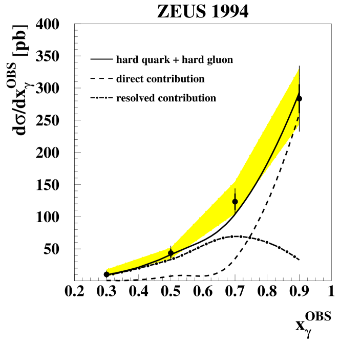
Fig. 97: Dijet production cross section in diffractive photoproduction in the range $134<W<277\,\mathrm{GeV}$, as a function of $x_{\gamma}^{OBS}$, for jets in the region $-1.5<\eta_{jet}<1$ and the most forward going hadron at $\eta_{\mathrm{max}}<1.8$ (solid dots). The solid line correspond to the Ingelman-Schlein model of the pomeron with a hard quark and gluon momentum distributions. Also shown is the resulting direct (dashed line) and resolved (dashed-dotted line) photon contributions. The shaded area represents the systematic error due to energy scale uncertainty.

The presence of both direct and resolved photon contributions has been established by studying the $x_{\gamma}^{OBS}$ distribution shown in Fig. 97. The direct processes populate the large $x_{\gamma}^{OBS}$ region, while the resolved processes tend to populate the lower $x_{\gamma}^{OBS}$ processes. A clear tail of the resolved processes is observed.

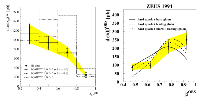
Fig. 98: Left - Jet production cross section in diffractive photoproduction in the range $150<W<250\,\mathrm{GeV}$ and $x_{{\scriptscriptstyle I\!\!P}}<0.05$, as a function of $z^{jets}_{x_{{\scriptscriptstyle I\!\!P}}}$. Right - Jet production cross section in diffractive photoproduction in the range $134<W<277\,\mathrm{GeV}$, as a function of $\beta^{OBS}$, for the most forward going hadron at $\eta_{\mathrm{max}}<1.8$ (solid dots). The lines correspond to the Ingelman-Schlein model of the pomeron with various momentum distributions of gluons. Left - fit 2 denotes a flat gluon distribution at the starting scale of $3\,\mathrm{GeV^{2}}$, while fit 3 denotes a leading gluon type of distribution. $<S>$ stands for survival probability. Right - as denoted in the figure. The shaded area represents the systematic error due to energy scale uncertainty.

The $\beta^{OBS}$ and the $z^{jets}_{x_{{\scriptscriptstyle I\!\!P}}}$ distributions are shown in Fig. 98. The comparison between the two figures demonstrates the restriction imposed by the $\eta_{\mathrm{max}}<1.8$ cut, which limits the invariant mass and the $x_{{\scriptscriptstyle I\!\!P}}$ of the selected events. For this restricted sample of events the distribution is seen to peak at large $\beta^{OBS}$, indicating that for these events the whole of the pomeron momentum is invested in the interaction.

The ZEUS results are well reproduced by a model with a soft factorisable pomeron with parton distributions obtained as the result of a combined fit to the DIS and photoproduction cross sections assuming both QCD and Regge factorization. Within the relatively large statistical and systematic errors, an acceptable description of the data is obtained, provided a large fraction of the pomeron momentum is carried by gluons.

Among the parton distributions which fit the $F_{2}^{D(3)}$ measurements of H1, the jet measurements prefer a gluon distribution which is flat at a scale of about $3\,\mathrm{GeV^{2}}$. However, even then the measured cross section seems to be systematically lower than expected. The agreement becomes better, if one assumes that the survival probability of a large rapidity gap is about $60\%$ (for discussion see section 6.7.2). Note that for $Q^{2}>7.5\,\mathrm{GeV^{2}}$ (?), the dijet cross section as a function of $z^{jets}_{x_{{\scriptscriptstyle I\!\!P}}}$ was found to be well reproduced, both in shape and normalization, with the ”flat” gluon distribution.

6.7.2 Large rapidity gaps between jets

One of the challenges of experimental physics is the search for the BFKL dynamics (?; ?; ?). It is by now well understood that in the presence of the interplay of soft and hard QCD phenomena it may be very difficult to uncover the BFKL dynamics if it exists. However, in hard reactions in which the $Q^{2}$ evolution is suppressed, the BFKL dynamics may be enhanced. An example of such a reaction is the exchange of a color-singlet between two jets with large transverse momenta. The requirement that both $p_{T}$ be large and approximately equal to $Q$ guarantees a large scale for perturbative calculations to be applicable and at the same time, prevents $Q^{2}$ evolution (?; ?; ?).

Theoretical background

In high energy hadronic collisions, the dominant mechanism for jet production is described by a hard scattering between partons from the incoming hadrons via a quark or gluon propagator. This propagator carries color charge. Since color confinement requires that the final state contains only color singlet objects, the exchange of color quantum numbers in the hard process means that a jet at some later stage generally exchanges color with another jet or beam remnant widely separated from it in rapidity. However, if hard scattering was mediated by the exchange of a color singlet propagator in the $t$-channel, each jet would be color connected only to the beam remnant closest in rapidity and the rapidity region between the jets would contain few final-state particles (?). The color singlet propagator could be an electroweak gauge boson or a strongly interacting object, and the soft gluon emission pattern produced in each case is similar (?) but the rates could be very different. In order to determine the rate of color singlet exchange processes, it has been proposed (?) to study the multiplicity distribution in pseudo-rapidity between the two jets.

Fig. 99: Diagrams for resolved photoproduction of jets via (a) color singlet exchange and (b) color non-singlet exchange. The topology of an event with a large rapidity gap between jets is shown in (c) where black dots represent final state hadrons and the boundary illustrates the acceptance of the detector.

An example of color singlet exchange in resolved photoproduction, in which a parton in the photon scatters from a parton in the proton via $t$-channel exchange of a color singlet object, is shown in Fig. 99a. An example of the more common color non-singlet exchange mechanism is shown in Fig. 99b. For high $E_{T}^{jet}$ dijet production, the magnitude of the square of the four-momentum ($|t|$) transferred by the color singlet object is large. Thus it is possible to calculate in perturbative QCD the cross section for the exchange of a strongly interacting color singlet object (?; ?; ?; ?). For instance, the ratio of the two-gluon color singlet exchange cross section to the single gluon exchange cross section has been estimated to be about 0.1 (?).

The event topology for the process of Fig. 99a is illustrated in Fig. 99c. There are two jets in the final state, shown as circles in ($\eta,\varphi$) space. For the color singlet exchange process, radiation into the region (labeled “gap”) between the jet cones is suppressed, giving rise to the rapidity gap signature. For color non-singlet exchange, the probability of finding no particles in the gap is expected to fall exponentially with increasing $\Delta\eta$, the distance in $\eta$ between the centres of the two jet cones.

HERA data

The search for rapidity gaps between jets has been performed by the ZEUS experiment for a sample of photoproduction events with at least two jets of $E_{T}^{jet}>6$ GeV in the $\gamma p$ centre of mass energy range $135<W_{\gamma p}<280\,\mathrm{GeV}$. The two highest transverse energy jets were required to have $\Delta\eta>2$ (i.e. cones not overlapping in $\eta$), $\eta^{jet}<2.5$ and boost $|(\eta_{1}+\eta_{2})|/2=|\bar{\eta}|<0.75$. These conditions constrain the jets to lie within the kinematic region where the detector and event simulations are best understood. The events with no particle of transverse energy $E_{T}^{particle}>300$ MeV within the $\eta$ space between the edges of the two highest $E_{T}^{jet}$ jet cones, are called gap events.

Fig. 100: The inclusive cross section as a function of the rapidity distance $\Delta\eta$ between jets (a) and for gap events (b). The data (black circles) are compared to MC expectations for a non-color singlet exchange in the jet production. The fraction is shown in (c) as a function of $\Delta\eta$ and redisplayed in (d) together with the results of a fit (full line) consisting of an exponential function (dotted line) and a constant (dashed line).

The inclusive cross section, $d\sigma/d\Delta\eta$, and the cross section for events with a gap, $d\sigma_{gap}/d\Delta\eta$, are presented in Fig. 100a and b as a function of $\Delta\eta$. The cross sections are compared to MC expectations based on the PYTHIA generator (?) which does not incorporate any color singlet exchange mechanism. The model gives a good description of the inclusive cross section at $\Delta\eta<3.5$ but an excess of events in the data is observed for larger $\Delta\eta$. The excess becomes more pronounced when the requirement of a gap is applied to the data and the MC model.

The gap-fraction, $f(\Delta\eta)$, is defined as the ratio of the number of dijet events at this $\Delta\eta$ which have a rapidity gap between the jets to the total number of dijet events at this $\Delta\eta$. The gap-fraction is shown in Fig. 100c and compared to the MC model. The data were fitted with a sum of an exponential and constant functions and the gap fraction for color singlet processes was found to be $f_{\mathrm{gap}}=0.07\pm 0.02^{+0.01}_{-0.02}$. The result of the fit is shown in Fig. 100d.

The excess in the gap-fraction over the expectation from non-singlet exchange may be interpreted as evidence for the exchange of a color singlet object. The fraction of gap events in photoproduction is larger than the values obtained for $p\bar{p}$ collisions (?; ?), which are $\sim 0.01$.

The fraction of events due to color singlet exchange, $\hat{f}(\Delta\eta)$, may be even higher than the measured excess. Secondary interactions of the photon and proton remnant jets could fill in the gap. A survival probability, ${\cal P}$, has been defined (?) which represents the probability that a secondary interaction does not occur. Then $f(\Delta\eta)=\hat{f}(\Delta\eta)\cdot{\cal P}$. Estimates of the survival probability for $p\bar{p}$ collisions at the Tevatron range from about 5% to 30% (?; ?; ?). The survival probability at HERA could be higher due to the lower centre-of-mass energy, or the fact that one remnant jet comes from a photon rather than a proton, or the fact that the mean fraction of the photon energy participating in the jet production in these events is high. Therefore the effect observed in photoproduction and $p\bar{p}$ jet production could arise from the same underlying process. The percentage of gap events in photoproduction is compatible with $\sim 0.10$ expected for two-gluon exchange mechanism.

6.8 Parton distributions in the pomeron

The QCD factorization theorem has been proven to be valid for the diffractive structure function $F_{2}^{D(3)}$ (?). The immediate consequence of this theorem is that the DGLAP evolution equation should describe the scaling violations observed in $F_{2}^{D(3)}$ and therefore the diffractive parton distributions can be derived, in a similar way as it is done for the inclusive $F_{2}$ of the proton. There is however no constraints on the gluon momentum distribution since the momentum sum rule, used for the proton structure function, does not formally apply.

The H1 experiment performed a QCD fit to their $F_{2}^{D(3)}$ measurements (?), assuming in addition the validity of Regge factorization with flux factors for the pomeron and the reggeon as determined from the data. The reggeon was assumed to have the parton content of the pion (?). The fit excluded the resonance region, $M_{X}<2\,\mathrm{GeV}$ and the data points which could be affected by a presence of a large longitudinal structure function component which was neglected in the measurements. The results of the fit were parameterizations of the parton distributions in the pomeron at a starting scaling $Q_{0}^{2}=3\,\mathrm{GeV^{2}}$.

Fig. 101: Quark and gluon momentum distributions in the pomeron as a function of the fraction of the pomeron momentum, $z$, for different fits to the $F_{2}^{D(3)}$ measurements. The results are evolved to different $Q^{2}$ values as denoted in the figure.

The data cannot be described by a parameterization in which the pomeron contains only quarks at $Q_{0}^{2}=3\,\mathrm{GeV^{2}}$. Various forms of the gluon distribution at the starting scale were explored. The best fit is obtained with a gluon distribution peaking at large $\beta$ as shown in Fig. 101. A flatter gluon distribution, albeit with worse $\chi^{2}$, can also describe the data. Note that the latter is preferred by the measurements of the dijet cross section (?). The quality of the fits can be seen in Figs. 86 and 87 where the measurements of $x_{{\scriptscriptstyle I\!\!P}}F_{2}^{D(3)}(x_{{\scriptscriptstyle I\!\!P}}=.003)$ as a function of $Q^{2}$ for fixed $\beta$ values and as a function of $\beta$ for fixed $Q^{2}$ values are compared to the expectations derived from the fit. The preferred solution is the one with a substantial gluon content in the pomeron. The relative fraction of the pomeron momentum carried by gluons is $\sim 90\%$ at $Q^{2}=4.5\,\mathrm{GeV^{2}}$ and decreases to $\sim 80\%$ at $Q^{2}=75\,\mathrm{GeV^{2}}$.

A similar conclusion has been reached by the ZEUS experiment (?) from a QCD fit to the $F_{2}^{D(3)}$ measurements and the diffractive dijet cross sections. The validity of Regge factorization was assumed with the pomeron flux as determined from soft interactions and in addition the QCD factorization theorem was assumed to be valid for diffractive dijet photoproduction. The last assumption has no theoretical foundation, with that this approach can be treated as a test for factorization breaking.

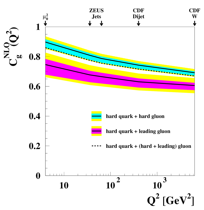
Fig. 102: Fraction of the pomeron momentum carried by gluons $c_{g}$ as a function of $Q^{2}$, determined from a NLO QCD fit to the $F_{2}^{D(3)}$ measurements and the diffractive dijet cross section in photoproduction.

A good fit to the data is found with a gluon distribution peaking at large $\beta$. Here the gluon distribution is constrained by the shape of the measured $\beta^{OBS}$ distribution. The relative fraction of the pomeron momentum carried by gluons, determined in $NLO$ approximation is shown in Fig. 102 as a function of $Q^{2}$ for various assumptions on the shape of the gluon distribution at a starting scale $Q_{0}^{2}=4\,\mathrm{GeV^{2}}$. The data require the fraction of the pomeron momentum carried by partons due to gluons to lie in the range $0.64<c_{g}^{NLO}<0.94$. The sensitivity of the data is not sufficient to prove or disprove the validity of the QCD factorization theorem for diffractive hard photoproduction.

The extrapolation of the ZEUS results to the $Q^{2}$ values probed in the measurements of hard diffractive processes in $p\bar{p}$ collisions is also consistent with the estimate of $70\pm 20\%$ by the CDF experiment (?). Note that this does not imply agreement in the total fraction of the pomeron momentum carried by partons, which is not constrained by any momentum sum rule and which has been found to be lower in $p\bar{p}$ collisions (?).

6.9 Conclusions and outlook

Hard diffractive interactions, in which the hadronic final state is separated from the proton by a large rapidity gap, have been observed in deep inelastic scattering and in high transverse momentum jet production in photoproduction. The interpretation of these data is in terms of a color singlet exchange, identified as the pomeron. The presence of a large scale allows to study the nature of this exchange in the language of partons and QCD. The measurements at HERA can be accounted for by a factorizable pomeron with a predominantly gluonic structure. Where available, also QCD inspired predictions describe the data well. The final verdict will have to await more precise measurements.

The quantitative and qualitative difference between diffraction in the presence of a hard scale and soft diffraction, and between hard diffraction in hadron-hadron and photon-hadron interactions may be the first sign that partons are not distributed uniformly inside the proton (?; ?). In addition, the sensitivity of hard diffractive processes to the transverse momenta of partons opens the possibility of investigating a three-dimensional color distribution in hadrons. The processes probed till now in QCD were only sensitive to the longitudinal dimension.

The diffractive phenomena have triggered a lot of new theoretical developments in QCD. It has brought to light the importance of color dynamics of QCD in understanding the nature of strong interactions. New phenomena such as color transparency in interactions of small size partonic configurations and color opacity in interactions of large size configurations are presently being discussed. They are essential in differentiating between hard processes which can be calculated in QCD and those where soft interactions still play an important role.

7 Vector meson production

There is a long experimental and theoretical history to the study of vector meson production. This study has found new vigor with the advent of HERA. On the experimental side, it is found that the cross sections for exclusive vector meson production rise strongly with energy when compared to fixed target experiments, if a hard scale is present in the process. This strong rise occurs although the reactions are very far from threshold. In the case of $J/\psi$ production, the strong rise of the cross section is measured directly in the HERA data. This steep rise in the cross sections was anticipated by some authors based on QCD inspired calculations. These calculations indicate that the cross sections depend on the square of the gluon density in the proton. If higher order calculations become available, the measurement of the energy dependence of the vector meson cross section may be the ideal method for measuring the gluon density in the proton.

In addition to being a probe of the gluon density, vector meson production tests our understanding of QCD for exclusive reactions in a domain where soft and hard physics merge. This is a region of fundamental importance, since basic physical realities such as the confinement of color are not at all understood. Vector meson production also offers an opportunity to study the properties of vacuum exchange in QCD, since no quantum numbers are exchanged in the scattering process. New experimental and theoretical results are becoming available at a rapid pace, and the study of vector meson production therefore promises to be a very fruitful one for the development of our understanding of QCD dynamics.

A word on terminology: at HERA, the reaction, $ep\rightarrow epV$, where $V$ represents a vector meson $(\rho,\;\omega,\;\phi,\;J/\psi,\;\Upsilon)$, is often referred to as elastic scattering. This is because the photon is viewed as fluctuating into a vector meson before the interaction with the proton, followed by a $Vp\rightarrow Vp$ scattering. The vector meson has the same quantum numbers as the photon, and is in some sense the “same” particle. However, at finite $Q^{2}$ this picture is no longer valid and the scattering is then no longer elastic. In this case, the process is often called exclusive vector meson production.

A comprehensive review of vector meson production at HERA has recently been published by ?.

7.1 Expectations for soft elastic scattering

7.1.1 Vector meson dominance model

Fig. 103: Elastic vector meson production in the vector dominance model (VDM). Here the photon is pictured as fluctuating into a vector meson which then scatters elastically from the proton via the exchange of a pomeron.

Light vector meson leptoproduction at small photon virtuality and small $W$ has been successfully explained as a three step process (see Fig. 103):

I) The incoming electron radiates a photon of small virtuality ($Q^{2}\approx 0$);

II) The photon fluctuates into a light vector meson, $V$, which carries the same quantum numbers as the photon; i.e.,${\rho,\omega,\phi}$;

III) The vector meson scatters elastically off the incoming proton via pomeron exchange.

This model (?), the so-called “Vector meson Dominance Model”, or VDM, gives good results when used, for example, to explain the total photon-proton cross section, $\sigma_{\gamma p}$, in terms of the total vector meson-proton cross section, $\sigma_{Vp}$ (see, e.g., ?),

$$\sigma_{\gamma p}\propto\sum_{\rho,\omega,\phi}A(f_{V})\sigma_{Vp}\;,$$ (188)

where $A(f_{V})$ is a known function of the coupling.

The $Q^{2}$ dependence of the $\gamma p\rightarrow Vp$ cross section can also be described by VDM,

$$\frac{d\sigma_{\gamma p\rightarrow Vp}}{d|t|}=\frac{d\sigma_{0}}{d|t|}\left(\frac{M_{V}^{2}}{M_{V}^{2}+Q^{2}}\right)^{2}\left({1+\epsilon\xi\frac{Q^{2}}{M_{V}^{2}}}\right)e^{-b|t|},$$ (189)

where $\sigma_{0}$ is the cross section at $Q^{2}=0$ , $\xi$ is the ratio of the longitudinal to transverse forward cross sections, $\epsilon$ is the ratio of the longitudinal to transverse photon flux of the virtual photon and $M_{V}$ is the mass of the vector meson; the distribution of $t$, the square of the four-momentum transfer between the photon and the vector meson, is experimentally described by a single exponential dependence, in the range from $t$ = 0 to $t$ = $-0.5$ GeV², with a slope parameter, $b\approx 7-12$ GeV^-2.

The differential cross section $d\sigma_{\gamma p\rightarrow Vp}/d|t|$ can be related to the total vector meson-proton cross section $\sigma_{Vp}$ by applying the optical theorem,

$$\left.\frac{d\sigma_{Vp\rightarrow Vp}}{d|t|}\right|_{t=0}=\frac{1+\eta^{2}}{16\pi}\sigma_{Vp}^{2},$$ (190)

where $\eta$ is the ratio of the real to the imaginary part of the forward $Vp$ scattering amplitude. Within VDM, elastic vector meson photoproduction is related to the elastic $Vp$ cross section; in particular, for $t=0$

$$\left.\frac{d\sigma_{\gamma p\rightarrow Vp}}{d|t|}\right|_{t=0}=\frac{4\pi\alpha}{f_{V}^{2}}\left.\frac{d\sigma_{Vp\rightarrow Vp}}{d|t|}\right|_{t=0},$$ (191)

where $4\pi\alpha/f_{V}^{2}$ is the probability for the $\gamma\rightarrow V$ transition.

Assuming that the real part of the amplitude is zero, as expected for purely diffractive scattering,

$${\left.\frac{d\sigma_{\gamma p\to Vp}}{d|t|}~{}\right|_{t=0}}=\frac{4\pi\alpha}{f_{V}^{2}}~{}\frac{1}{16\pi}\,{\sigma}^{2}_{Vp}\,.$$ (192)

A measurement of $d\sigma_{\gamma p\to Vp}/d|t|$ can therefore be used to calculate $\sigma_{Vp}$.

As discussed in section 4.1, hadronic cross sections, and the total photoproduction cross section, have been measured to have an energy dependence

$$\sigma_{\gamma p}\sim\sigma_{\pi p}\sim W^{2\cdot 0.08}\;.$$ (193)

Assuming that the $Vp$ cross section has the typical behavior of hadronic cross sections, VDM therefore predicts

$${\left.\frac{d\sigma_{\gamma p\to Vp}}{d|t|}~{}\right|_{t=0}}\sim\sigma_{Vp}^{2}\sim W^{0.32}\;.$$ (194)

7.1.2 Regge Theory expectations

In Regge Theory, we expect the $\gamma p\rightarrow Vp$ cross section to have the form

$$\frac{d\sigma_{\gamma p\rightarrow Vp}}{d|t|}\propto e^{-b_{0}|t|}\left(\frac{W^{2}}{W^{2}_{0}}\right)^{2(\alpha(t)-1)}\;,$$ (195)

where $\alpha(t)$ is the pomeron trajectory. Phenomenological fits (?) to fixed target and hadron-hadron scattering data have determined that $\alpha(t)$ can be parameterized by a linear form,

$$\alpha(t)=\alpha_{0}+\alpha^{\prime}t\;,$$ (196)

with parameters

$$\alpha_{0} = 1.08\;,$$ (197)

$$\alpha^{\prime} = 0.25\;{\rm GeV}^{-2}.$$ (198)

The fact that $\alpha^{\prime}$ is non-zero means that the slope of the $t$ distribution will depend on the energy as

$$b=b_{0}+2\alpha^{\prime}\ln\frac{W^{2}}{W^{2}_{0}}\;,$$ (199)

while the $W$ dependence will depend on $t$. Denoting $\delta$ as the power of $W$ ($d\sigma/dt\propto W^{\delta}$), we have

$$\delta=4(\alpha_{0}+\alpha^{\prime}t-1)\;.$$ (200)

Integrating over $t$ gives

$$\sigma=\frac{W^{4(\alpha_{0}-1)}}{b}\;,$$ (201)

which results in an effective power of the $W$ dependence of

$$\delta\approx 4(\alpha_{0}-\frac{\alpha^{\prime}}{b}-1)\;,$$ (202)

where $b$ depends on $W$ as shown above. There is no prediction on the value of $b$ from Regge theory - the parameters $b_{0},\;W_{0},{\rm and}\;\alpha^{\prime}$ could all be process dependent, and could also be $Q^{2}$ dependent for a given process. Typically, values of $b=10$ GeV^-2 are found in soft processes, leading to an expectation of $\delta=0.22$ for $\alpha^{\prime}=0.25$ GeV^-2. In processes with a hard scale, measured $b$ values are considerably smaller. For $b=5$ GeV^-2, the expectation is $\delta=0.12$.

In a geometrical picture, the slope of the $t$ dependence can be interpreted as giving the size of the scattering objects,

$$b\propto{R_{p}^{2}}+{R_{\gamma}^{2}}\;,$$ (203)

where $R_{p}$ is the effective proton radius and $R_{\gamma}$ is the effective size of the $\gamma$ induced state scattering on the proton. For $b=8$ GeV^-2, $\sqrt{R_{p}^{2}+R_{\gamma}^{2}}\approx 1$ fm.

The $t$ dependence has been studied experimentally as a function of $Q^{2}$ and $W$. It is seen that the slope $b$ decreases with $Q^{2}$, indicating that the photon is becoming more point-like as the virtuality increases. The tendency for $b$ to increase with $W$ has been called “shrinkage” although, in the geometrical picture, a steeper $t$ dependence corresponds to the scattering of larger objects.

7.2 Expectations in the presence of a hard scale

7.2.1 Non-perturbative approach

The non-perturbative methods are essentially attempts to extend Regge Theory to reactions where a hard scale is present. Many such models have been constructed. ? gives a review of these. We will focus in this review on pQCD inspired models as they contain more dynamics, and generally make more quantitative predictions. A focus of the HERA VM studies is to determine at which scale, and for which reactions, the pQCD approach gives a better description of the data than the pomeron model.

7.2.2 Outline of pQCD approaches

In the past few years, new calculations of diffractive vector meson production, using perturbative QCD, have been performed by many authors. We give here a description of the general features of the pQCD models.

Fig. 104: Exclusive vector meson production in QCD based models. Here the photon is viewed as fluctuating into a quark-antiquark pair. These then couple to the proton via the exchange of two gluons (with momentum fractions $x_{1},x_{2}$). The vector meson is formed after the scattering has occurred.

In pQCD models, the scattering (${\gamma p\rightarrow Vp}$) is viewed, in the proton rest frame, as a sequence of events very well separated in time (?). The process is depicted in Fig. 104. The steps are:

I) The photon fluctuates into a $q\bar{q}$ state,

II) the $q\bar{q}$ pair scatters on the proton target,

III) the scattered $q\bar{q}$ pair turns into a vector meson.

The proton target acts as a source of color fields and the interaction with the quark-antiquark pair is mediated by the exchange of two gluons in a color singlet state. According to this picture, diffractive production of vector mesons in the presence of a hard scale probes the gluonic content of the proton. The scale $\mu$ at which $\alpha_{s}$ and the gluon density are evaluated can depend on the photon virtuality $Q^{2}$, on the mass of the vector meson M_V and on the $4$-momentum transfer at the proton vertex, $t$;

$$\mu^{2}=f(M_{V}^{2},Q^{2},t)\;,$$ (204)

with different models using different ansätze. This formalism can be applied to photoproduction events if $M_{V}$ is large enough.

$J/\psi$ production in pQCD

? has calculated the cross section for diffractive photo- and electroproduction of $J/\psi$ mesons within the $\alpha_{s}\ln\frac{1}{x}$ approximation and in a constituent quark model approximation for the wave function of the $J/\psi$. In this model, the scale of the interaction is given by

$$\mu^{2}=\frac{Q^{2}+m_{J/\psi}^{2}+|t|}{4}\;.$$ (205)

In photoproduction at small $t$, the scale would therefore take on the value $\mu^{2}=2.4$ GeV². Using a gluon density with an $x$ dependence given by $x^{-0.2}$ at small-$x$ would results in a cross section dependence $\sigma_{\gamma p\rightarrow J/\psi p}\propto W^{0.8}$ at large $W$, a much steeper dependence than expected from Regge Theory.

The calculation was extended beyond leading log (?) and compared to HERA data. It was found that, although large normalization uncertainties remain, this process is indeed very sensitive to the form of the gluon density in the proton.

Electroproduction of vector mesons

In DIS, the cross section is predicted to be dominated by longitudinally polarized virtual photons scattering into longitudinally polarized vector mesons (?; ?; ?). The cross section has been calculated in leading $\alpha_{s}\ln\frac{Q^{2}}{\Lambda^{2}}\ln\frac{1}{x}$ approximation (?) for vector mesons built of light flavors, and reads

$$\left.\frac{{\rm d}\sigma_{L}}{{\rm d}t}\right|_{t=0}=\frac{A}{Q^{6}}\alpha_{s}^{2}(Q^{2})\left|\left(1+\frac{i\pi}{2}\frac{{\rm d}}{{\rm d}\ln x}\right)xg(x,Q^{2})\right|^{2}\,,$$ (206)

where $A$ is a constant which depends on the VM wave function. Within this theoretical framework the measurement of $\left.{\rm d}\sigma/{\rm d}t\right|_{t=0}$ for vector meson electroproduction provides a probe for the gluon content in the proton, which is sensitive to the square of the gluon density. Different types of vector mesons can be used for independent measurements that can be compared to the theoretical predictions.

We review some of the expectations of the cross sections:

• The cross section contains a $1/Q^{6}$ factor. However, the $Q^{2}$ dependencies of $\alpha_{s}$ and the gluon density also need to be taken into account. These compensate some of the fall off at small $x$. The effective $Q^{2}$ dependence using CTEQ3L (?) and the LO form for $\alpha_{s}$ is found to be $d\sigma/dt\propto 1/Q^{5}$, with a weak $x$ dependence.

  The calculation presented in ? has been redone in leading $\alpha_{s}\ln\frac{Q^{2}}{\Lambda^{2}}$ approximation (?). In this work, among other improvements, the Fermi motion of the quarks in the vector meson has been considered. The net effect is to reduce the steepness of the $Q^{2}$ dependence and to delay the onset of the asymptotic regime. Precise measurements could therefore in principle yield information on the wave function of the vector mesons.

• In the pQCD calculations, there is no coupling of the $t$ and $W$ dependences, such that no shrinkage is expected. The lack of shrinkage, along with the prediction of a steep $W$ dependence, are telltale signs that the reaction is predominantly driven by perturbative processes.

• The cross section presented above is for longitudinally polarized photons. The authors (?) expect that this is the dominant contribution to the cross section in DIS.

  The region of validity of the pQCD calculations has been investigated be several authors. In ?, it is argued that the region of validity of the pQCD calculations is signaled by the exclusively longitudinal polarization of the vector meson. The reason for this (?) is that longitudinally polarized photons will preferentially produce $q\bar{q}$ pairs which are symmetric in longitudinal momentum, and therefore have large $k_{T}$, while transverse photons will produce asymmetric pairs in longitudinal momentum, and correspondingly small $k_{T}$. In the latter case, the scattering is dominantly soft (see the discussion in section 2.8).

  A recent pQCD calculation for $\rho^{0}$ electroproduction (?) based on the open production of light $q\overline{q}$ pairs and parton-hadron duality gives an estimate of the transverse photon contribution to the $\gamma^{*}p\rightarrow Vp$ cross section. It is found that the transverse cross section does not drop off as fast as would be predicted from a convolution of the vector meson wave function. In fact, the authors claim that a convolution of the type $<q\overline{q}|\rho^{0}>$ is wrong and cannot reproduce the data. Rather, confinement forces the $q\overline{q}$ into a $\rho^{0}$ long after the interaction with the proton.

• The interaction should be flavor independent at high enough scales. From the quark charges of the vector mesons and a flavor independent production mechanism, the exclusive production cross section is expected to have relative size $9:1:2:8$ for $\rho^{0}:\omega^{0}:\phi:J/\psi$. This expectation is badly broken at small $Q^{2}$, where the heavier vector mesons are strongly suppressed. The pQCD predictions change the ratio somewhat due to wave function effects, such that the relative contribution from heavier vector mesons is modified (?) at large $Q^{2}$.

Vector meson production at large $t$

In (?; ?), it is pointed out that the hard scale necessary for the pQCD calculations to be valid can also be provided by $t$, and that, at large $t$, the BFKL equation can be used to predict the slope of both the $W$ and $t$ dependencies. Recent QCD calculations predict that light vector mesons produced at large $t$ in proton dissociative production should have zero helicity (?), independent of the initial photon polarization.

7.3 Pre-HERA experimental results

A comprehensive review of results from photoproduction of vector mesons prior to 1978 can be found in ?. These measurements show, at energies up to $20$ GeV, a weak dependence of the cross sections on energy, similar to those found in hadron-hadron scattering. The $t$ dependence of the data can be characterized by an exponential at small $t$, $d\sigma/d|t|\propto exp(-b|t|)$, and the $Q^{2}$ dependence is well described by VDM (see Eq. (189)). Also, the helicity of the vector meson is similar to that of the incident photon, i.e. s-channel helicity is largely conserved (SCHC).

At larger $Q^{2}$, leptoproduction results have been presented by EMC (?; ?), NMC (?; ?) and E665 (?). In these measurements, the $Q^{2}$ range extends up to $25$ GeV² and $W$ extends to $28$ GeV. The data are generally consistent with a $1/Q^{4}$ behavior, the $|t|$ slope is found to be much shallower than in photoproduction (the NMC Collaboration (?) has measured $b=4.6\pm 0.8$ GeV^-2 for $Q^{2}>6$ GeV²), the fraction of longitudinally polarized $\rho^{0}$’s increases beyond $50$ % at the highest $Q^{2}$ probed, and no significant $W$ dependence of the cross sections is found.

7.3.1 Comment on Vector Meson Data

It should be mentioned that the experimental results on $\rho^{0}$ production are not always consistent. For example, NMC measurements (?) disagree with EMC measurements (?; ?) as to the $Q^{2}$, $t$, and angular dependencies of the data. The recent cross section measurements by E665 are considerably higher than those from the NMC collaboration, and the H1 and ZEUS collaborations have widely differing cross sections for $\rho^{0}$ electroproduction. The problems likely stem from two main sources:

1. The difficulty in defining the $\rho^{0}$ signal. The resonance is broad, and must be integrated over a fixed range. The contribution from non-resonant $\pi^{+}\pi^{-}$ production or background under the resonance is very difficult to estimate.

2. The uncertainty in the contribution from proton dissociation reactions. This background is difficult to estimate since a large fraction of the events with proton dissociation look in the detector like elastic events, and there is no good model describing the properties of the proton dissociation system.

Given these difficulties, comparison of data sets from different measurements should be performed with care, as they could lead to erroneous conclusions.

7.4 HERA results

7.4.1 Kinematics of vector meson production at HERA

In addition to the standard DIS variables, several extra variables are needed to describe vector meson production in the reaction,

$$e~{}p\rightarrow e~{}V~{}+Y\,,$$ (207)

where $Y$ represents either a proton or a diffractively dissociated proton remnant of mass $M_{Y}$:

• $t^{\prime}=|t~{}-~{}t_{min}|$, where $t$ is the four-momentum transfer squared, $t$ = $(q-v)^{2}=(P-P^{\prime})^{2}$, from the photon to the $\rho^{0}$ (with four-mqomentum $v$), $t_{min}$ is the minimum kinematically allowed value of $t$ and $P^{\prime}$ is the four-momentum of the outgoing proton. The squared transverse momentum $p_{T}^{2}$ of the $\rho^{0}$ with respect to the photon direction is a good approximation to $t^{\prime}$,

• the three angles $\Phi$, $\phi_{h}$, and $\theta_{h}$, described below.

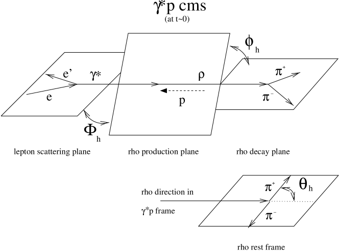
Fig. 105: A graphical description of the angles needed to analyze the helicity states of the vector meson (here denoted as $\rho$): $\theta_{h}$ is the polar angle in the helicity system, $\phi_{h}$ the angle between the $\rho$ decay and production plane, and $\Phi_{h}$ the angle between the lepton scattering and $\rho$ production planes.

The production and decay angles are usually defined in the s-channel helicity frame (?), as shown in Fig. 105. The vector meson direction in the $\gamma^{*}p$ frame is taken as the quantization axis, and, in the case of a two-body decay, the direction of one of the particles in the rest frame of the vector meson is used to calculate $\theta_{h},\phi_{h}$. In the case of a three-body decay, the normal to the decay plane is used to define the decay angles. The angle $\Phi$ between the vector meson production plane and the electron scattering plane in the $\gamma^{*}p$ rest frame is also used. The full decay angular distribution is usually expressed in terms of $(\cos\theta_{h},\phi_{h},\Phi)$. In the case where the electron beam is not longitudinally polarized, the electron beam energy is not varied, and s-channel helicity conservation (SCHC) is assumed to apply, the decay distribution reduces to (for a decay into two spin-0 particles),

$$W(\cos\theta_{h},\psi_{h})=\frac{3}{4\pi}\left[\frac{1}{2}(1-r_{00}^{04})+\frac{1}{2}(3r_{00}^{04}-1)\cos^{2}\theta_{h}\right.$$

$$\!\!\!\!\!\left.\mbox{ }+\epsilon r_{1-1}^{1}\sin^{2}\theta_{h}\cos 2\psi_{h}-2\sqrt{\epsilon(1+\epsilon)}Re[r_{10}^{5}]\sin 2\theta_{h}\cos\psi_{h}\right],$$

where $\psi_{h}=\phi_{h}-\Phi$ and $r_{00}^{04},\;r_{1-1},\;Re[r_{10}^{5}]$ are the non-zero combinations of the vector meson spin density matrix elements. The parameter $\epsilon$ is the ratio of the longitudinal to transverse photon flux. $r_{00}^{04}$ gives the probability that the vector meson is produced in a helicity zero state, and, if s-channel helicity holds, is related to the ratio of the longitudinal to transverse photon cross sections as

$$R = \frac{\sigma_{L}}{\sigma_{T}}$$ (209)

$$= \frac{r_{00}^{04}}{\epsilon(1-r_{00}^{04})}\;\;\;.$$ (210)

The matrix element $r_{1-1}^{1}$ determines the anisotropy of the $\psi_{h}$ distribution, while $Re[r_{10}^{5}]$ is related to the interference between the production amplitudes by longitudinal and transverse photons (?). Taking the one dimensional projections in $\cos\theta_{h}$ and $\phi_{h}$ gives

$$\frac{1}{N}\frac{dN}{d\cos\theta_{h}} = \frac{3}{4}[1-r_{00}^{04}+(3r_{00}^{04}-1)\cos^{2}\theta_{h}],$$ (211)

$$\frac{1}{N}\frac{dN}{d\psi_{h}} = \frac{1}{2\pi}(1+2\epsilon r^{1}_{1-1}\cos 2\psi_{h})\;\;\;.$$ (212)

If, in addition to SCHC, the exchange has so-called natural parity, then the further relationship holds

$$r^{1}_{1-1}=\frac{1}{2}(1-r_{00}^{04})\,.$$ (213)

7.4.2 Experimental analysis

The analysis of vector meson production is at first sight quite straightforward. Events are searched for with typically two or three isolated tracks and no extra energy depositqs in the calorimeter (e.g., $ep\rightarrow e~{}\rho~{}p,\;\rho\rightarrow\pi^{+}\pi^{-}$, where the electron is in the detector in the case of DIS, and escapes down the beampipe in the case of photoproduction.) The momenta from the tracks are then used to reconstruct an invariant mass, and events are kept where the reconstructed mass is near the mass of the particle under study. The kinematics are generally reconstructed very precisely. In DIS, the variables ($Q^{2},y,\;p_{T}^{2},\;M_{V},\;\Phi,\;\phi_{h},\;\theta_{h}$) can all be reconstructed, while in photoproduction, the angle $\Phi$ is unmeasurable because the scattered electron is typically not observed. The complication in the analysis comes from the fact that the acceptance depends, to varying extent, on all kinematic variables. It is therefore important to have Monte Carlo simulations which are capable of reproducing the data to have confidence in the results.

It is usually required to see the decay tracks of the vector meson in the central tracking detectors to perform a full reconstruction of the events. This limits the $W$ range of the measurements to typically $40<W<140$ GeV. The $Q^{2}$ range up to $50$ GeV² has been measured, limited by the steep drop of the cross section with $Q^{2}$. The $t$ dependence is also steep, and at large $|t|$ backgrounds from proton dissociation are important. This generally limits analyses to the range $|t|<0.6$ GeV². Measurements have also been performed for the proton dissociation events, in which case larger $|t|$ values are used.

The cross sections of interest are the $\gamma^{*}p$ cross sections. These are derived from the $ep$ cross sections starting with the differential form of the $ep$ cross section,

$$\frac{d\sigma_{ep\rightarrow epV}}{dydQ^{2}}=\Gamma(\sigma_{T}+\epsilon\sigma_{L})\,,$$ (214)

where

$$\Gamma=\frac{\alpha}{2\pi yQ^{2}}\left(Y_{+}-2(1-y)\frac{Q^{2}_{min}}{Q^{2}}\right)$$ (215)

and

$$\epsilon=\frac{2(1-y)}{Y_{+}-2(1-y)\frac{Q^{2}_{min}}{Q^{2}}}\;.$$ (216)

$Q^{2}_{min}=m_{e}^{2}\frac{y^{2}}{(1-y)}$ is the minimum possible $Q^{2}$ and $Y_{+}=1+(1-y)^{2}$.

• In photoproduction, the behavior of the cross section is assumed to follow the VDM form, given in Eq. (189),

  $$\sigma_{T}(y,Q^{2}) = \left(\frac{M_{V}^{2}}{Q^{2}+M_{V}^{2}}\right)^{2}\sigma_{T}(y,Q^{2}=0)\,,$$ (217)

  $$\sigma_{L}(y,Q^{2}) = \frac{Q^{2}}{M_{V}^{2}}\sigma_{T}(y,Q^{2})\;.$$ (218)

  The $y$ dependence is expected to be slow (recall that $y=W^{2}/s$). In this case, we can extract $\sigma_{T}$ from

  $$\int_{y_{min}}^{y_{max}}dy\int_{Q^{2}_{min}}^{Q^{2}_{max}}dQ^{2}\frac{d\sigma_{ep\rightarrow epV}}{dydQ^{2}}=$$

  $$\!\!\!\!\!\!\!\sigma_{T}(\bar{y},Q^{2}=0)\!\!\!\int_{y_{min}}^{y_{max}}\!\!\!\!\!dy\int_{Q^{2}_{min}}^{Q^{2}_{max}}\!\!\!dQ^{2}\Gamma\left(\!\!\frac{M_{V}^{2}}{Q^{2}+M_{V}^{2}}\!\!\right)^{2}\!\!\left(\!1+\epsilon\frac{Q^{2}}{M_{V}^{2}}\!\right).$$

• In the case of heavy quark production, or vector meson production in DIS, we can no longer assume that the $y$ (or $W$) dependence will be weak. In this case, we need a model for the $\gamma p$ cross section, which has to be tuned to the data, before the cross sections can be extracted. This procedure is very similar to the extraction of $F_{2}$.

7.4.3 Backgrounds

The final state for vector meson production is very clean, and the background from non-vector meson final states is usually negligible. However, the cross sections of interest are either the elastic or the proton-dissociative cross sections. These are very difficult to disentangle, since the proton is often excited to a small mass state which is not distinguishable from elastic reactions in the detectors. Models are then needed to extrapolate from the high mass tail, which can be identified in the detectors, to the full mass range for the proton-dissociative system. This correction can be quite large (of order 25 %), and can therefore lead to uncertainties in the overall normalization of the elastic cross section. The $t$ slopes of the two reactions are also considerably different, such that the extracted $t$ dependence is also quite sensitive to the estimated contributions.

7.4.4 Light vector meson photoproduction

A large amount of data exists from pre-HERA times on light vector meson photoproduction (see, e.g., ?). It is interesting to test how these results extrapolate to the much higher center-of-mass energies available in photoproduction at HERA. Results exist from HERA on the photoproduction of light vector mesons for $\rho^{0}$, $\omega^{0}$ and $\phi$. The data sets are summarized in Table 6. In the following sections, we discuss the mass, $W$ and $t$ dependencies of the cross sections, and review the tests of s-channel helicity conservation.

Table 6: Summary of results on cross sections and $t$ slopes from the elastic photoproduction of light vector mesons at small $t$ at HERA. The different symbols are defined in the text. The $\gamma p$ cross sections quoted are for the $t$ range specified in the table.

Reaction	$<\!W\!>$	$\sigma_{\gamma p\rightarrow Vp}$	$|t|$-range	$b$	comment
studied	(GeV)	($\mu$b)	(GeV2)	(GeV-2)
$\rho^{0}\rightarrow\pi^{+}~{}\pi^{-}$	$70$	$14.7\pm 0.4\pm 2.4$	$<0.50$	$9.9\pm 1.2\pm 1.4$	(?)
$\rho^{0}\rightarrow\pi^{+}~{}\pi^{-}$	$55$	$9.1\pm 0.9\pm 2.5$	$<0.50$	$10.9\pm 2.4\pm 1.1$	(?)
	$187$	$13.6\pm 0.8\pm 2.4$
$\rho^{0}\rightarrow\pi^{+}~{}\pi^{-}$	$73$	$5.8\pm 0.3\pm 0.7$	$0.073-0.40$	$9.8\pm 0.8\pm 1.1$	(?)
$\rho^{0}\rightarrow\pi^{+}~{}\pi^{-}$	$55$	$10.9\pm 0.2^{+1.5}_{-1.3}$	$<0.50$	$10.9\pm 0.3^{+1.0}_{-0.5}$	fit form
	$65$	$10.8\pm 0.2^{+1.3}_{-1.1}$			$d\sigma/d|t|=e^{-b|t|+ct^{2}}$
	$75$	$11.4\pm 0.3^{+1.0}_{-1.2}$			(?)
	$90$	$11.7\pm 0.3^{+1.1}_{-1.3}$
$\omega^{0}\rightarrow\pi^{+}~{}\pi^{-}~{}\pi^{0}$	$80$	$1.21\pm 0.12\pm 0.23$	$<0.60$	$10.0\pm 1.2\pm 1.3$	(?)
$\phi\rightarrow K^{+}~{}K^{-}$	$70$	$0.96\pm 0.19^{+0.21}_{-0.18}$	$<0.50$		(?)

Mass spectra

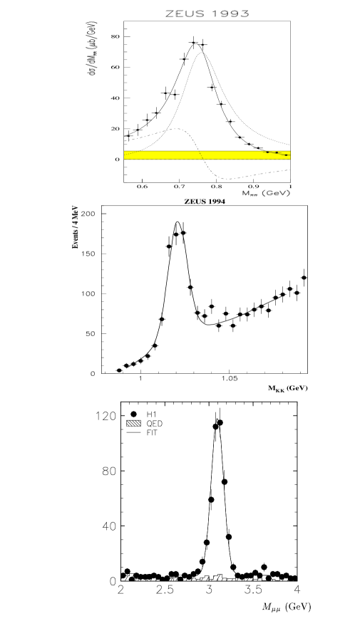
Fig. 106: Typical mass distribution observed in photoproduction for the $\rho^{0}\rightarrow\pi^{+}\pi^{-}$ signal (top), the $\phi\rightarrow K^{+}K^{-}$ signal (center), and the $J/\psi\rightarrow\mu^{+}\mu^{-}$ signal (bottom). In the case of the $\rho^{0}$, the dotted curve represents the resonant Breit-Wigner contribution and the dot-dashed curve the interference term; the shaded band represents the size of the uncertainty on the background term. The continuous curve is the sum of the contributions.

Typical mass distributions are shown in Fig. 106. Clear peaks are seen in all cases. The $\phi$ and $J/\psi$ mass distributions are narrow, and the backgrounds under the peak are extracted in a straightforward way by fitting the distributions with Gaussians or Gaussians+Breit-Wigner functions for the peaks and polynomial functions for the background. In the case of the $\rho^{0}$, the mass spectrum is quite broad, and care has to be taken in extracting the resonant contribution.

The mass distribution of the $\rho^{0}$ is skewed compared to a Breit-Wigner distribution, as seen in Fig. 106: there is an enhancement of the small mass side and a suppression of the high mass side. This distribution can be understood in terms of the interference between the resonant $\pi^{+}\pi^{-}$ production and a non-resonant background as discussed by ?. The resonant production is described by a relativistic p-wave Breit-Wigner function,

$$BW_{\rho}(M_{\pi\pi})=\frac{M_{\pi\pi}m_{\rho}\Gamma_{\rho}(M_{\pi\pi})}{(M_{\pi\pi}^{2}-m_{\rho}^{2})^{2}+m_{\rho}^{2}\Gamma_{\rho}^{2}(M_{\pi\pi})}\,,$$ (220)

with a momentum dependent width (?)

$$\Gamma_{\rho}(M_{\pi\pi})=\Gamma_{0}\left(\frac{p^{*}}{p^{*}_{0}}\right)^{3}\frac{m_{\rho}}{M_{\pi\pi}}\,,$$ (221)

where $\Gamma_{0}$ is the width of the $\rho^{0}$, $p^{*}$ is the $\pi$ momentum in the $\pi^{+}\pi^{-}$ rest frame and $p^{*}_{0}$ is the value of $p^{*}$ at the $\rho^{0}$ nominal mass $m_{\rho}$.

Parameterizations are then used for the background and interference terms which are added to the Breit-Wigner in order to describe the mass spectrum. In this way, fits can be performed which reproduce the standard values for the $\rho^{0}$ mass and width; viz., $m_{\rho}=0.770$ GeV and $\Gamma_{0}=150$ MeV (?). An example of such a fit is given in Fig. 106, where the different terms are described.

Different assumptions for the functional form of $d\sigma/dM_{\pi\pi}$ are often used. One common form is that proposed ?,

$$\frac{d\sigma}{dM_{\pi\pi}}=f_{\rho}\cdot BW_{\rho}(M_{\pi\pi})\cdot(m_{\rho}/M_{\pi\pi})^{k}+f_{PS},$$ (222)

Fig. 107: The Ross-Stodolsky parameter $k$ as a function of $|t|$. The ZEUS data are compared to results from fixed target experiments (?; ?) and show the same trend.

where the factor $(m_{\rho}/M_{\pi\pi})^{k}$ accounts for the skewing of the shape of the $\rho^{0}$ signal. The background term $f_{PS}$ is usually taken to be constant. The value of $k$ is then a measure of the skewing. This value is given in Fig. 107 as a function of $|t|$. It is seen that the skewing is reduced when $|t|$ is increased.

$t$ dependence

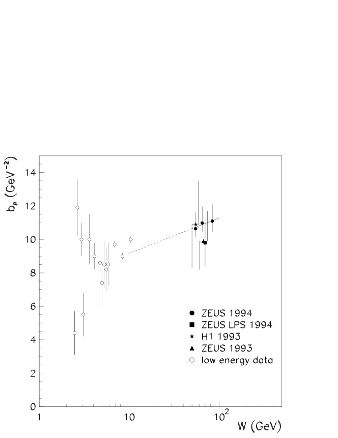
Fig. 108: The slope $b$ for elastic $\rho^{0}$ photoproduction. The line is the result of a fit of the form $b=b_{0}+2\alpha^{\prime}ln(W^{2}/W_{0}^{2})$. The fit is performed to the ZEUS data, and extrapolated down to the fixed target measurements.

The $t$ slopes are summarized in Table 6. As can be seen, values around $b=10$ GeV^-2 are measured. The development of $b$ with $W$ is shown for $\rho^{0}$ photoproduction in Fig. 108. The results from fixed target experiments are shown along with the HERA data. A fit of the form $b=b_{0}+2\alpha^{\prime}\ln(W^{2}/W_{0}^{2})$ was performed on the ZEUS data (?), resulting in $\alpha^{\prime}=0.23\pm 0.15^{+0.10}_{-0.07}\,\mathrm{GeV^{-2}}$. The result is compatible with the presence of shrinkage, but the large errors on $\alpha^{\prime}$ precludes any definitive statement.

The $|t|$ slope has been measured as a function of the invariant mass of the $\pi^{+}~{}\pi^{-}$, and found to decrease in accord with results from previous measurements (?).

$W$ dependence

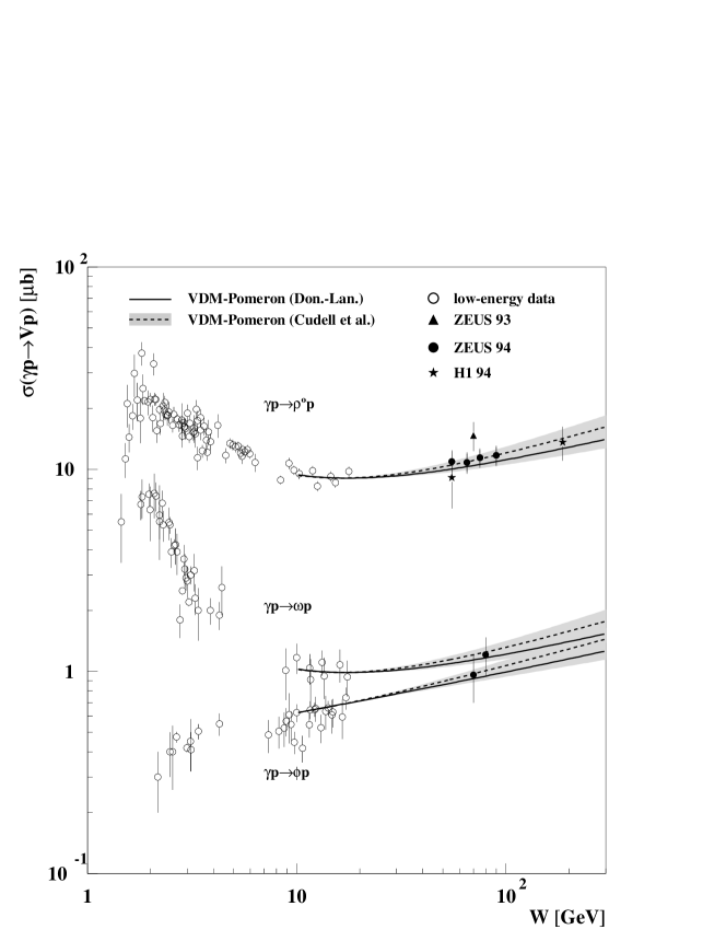
Fig. 109: The elastic vector meson photoproduction cross sections as functions of $W$ for $\rho^{0},\;\omega$ and $\phi$. The solid curve is for the pomeron model of ? while the dashed curve is based on an updated version by ?. The error band specifies the range of expectations in the Cudell model.

The $W$ dependence of the cross sections are shown in Fig. 109. Given a typical $t$ slope of $b=10$ GeV^-2, the Regge theory expectation for the exponent of $W$ in the cross section is (see Eq. (200))

$$\delta=4(1.08-\frac{0.25}{10}-1)=0.22$$ (223)

If the more recent value of $\alpha_{0}=1.096^{+0.012}_{-0.009}$ from ? is taken, then the expected $W$ slope is $\delta=0.28^{+0.05}_{-0.04}$. These two expectations are shown in the figure. They are both in good agreement with the data.

Test of SCHC

As described above, the angle $\Phi$ is not measured in photoproduction. Integrating over this angle, the distribution in the remaining two angles is

$$W(\cos\theta_{h},\phi_{h})=\frac{3}{4\pi}\left[\frac{1}{2}(1-r^{04}_{00})+\frac{1}{2}(3r^{04}_{00}-1)\cos^{2}\theta_{h}\right.$$ (224)

$$\mbox{}-\sqrt{2}Re[r^{04}_{10}]\sin 2\theta_{h}\cos\phi_{h}\left.\mbox{}-r^{04}_{1-1}\sin^{2}\theta_{h}\cos 2\phi_{h}\right]\;.$$

Fig. 110: The differential distributions in $cos\theta_{h}$ and $\phi_{h}$ for the reaction $\gamma p\rightarrow\rho^{0}p$.

The element $r^{04}_{1-1}$ is related to the size of the interference between the helicity non-flip and double-flip amplitudes, while $qRe[r^{04}_{10}]$ is related to the interference between the helicity non-flip and single flip amplitudes. As mentioned above, $r^{04}_{00}$ is the probability to find the $\rho^{0}$ with helicity $0$. If SCHC holds, then both $r^{04}_{1-1}$ and $Re[r^{04}_{10}]$ should be zero. In addition, $r^{04}_{00}$ is expected to be small since the photon is predominantly transversely polarized. Typical distributions for $\cos\theta_{h}$ and $\phi_{h}$ are shown in Fig. 110, along with the result of a fit using Eq. (224). For this particular result (?), the fitted matrix elements are

$$r^{04}_{00} = 0.01\pm 0.01\pm 0.02\;,$$ (225)

$$r^{04}_{1-1} = -0.01\pm 0.01\pm 0.01\;,$$ (226)

$$Re[r^{04}_{10}] = 0.01\pm 0.01\pm 0.01\;,$$ (227)

in good agreement with expectations from SCHC. This conclusion is generally true for all photoproduction measurements.

Proton dissociation results

The ZEUS experiment has also measured the $|t|$ dependence for $\gamma p\rightarrow\rho^{0}N$, where $N$ represents a small mass baryonic state from proton dissociation. In this case, the $t$ slope is measured to be about $b=6$ GeV^-2 (?); i.e., about half the value found for elastic $\rho^{0}$ production. A smaller value of $b$ is expected since the reaction is now inelastic on the proton side, with a smaller effective radius.

7.4.5 $J/\psi$ and $\Upsilon$ photoproduction

The reaction $\gamma p\rightarrow J/\psi Y$ has been measured at HERA for several different cases:

1. The system Y consists of a single proton. This is the so-called elastic reaction.

2. The system Y consists of a small mass system stemming from the dissociation of the proton.

3. Inelastic production, generated by photon-gluon fusion, or resolved photon-parton scattering.

Inelastic $J/\psi$ production has been described in section 4.4. We focus here on cases 1,2. The recent results on $\Upsilon$ photoproduction are discussed at the end of the section.

A summary of the different data sets available on $J/\psi$ photoproduction from HERA is given in Table 7.

Table 7: Summary of results on cross sections and $t$ slopes from the elastic (and proton dissociation) photoproduction of $J/\psi$ mesons at HERA. The comments apply to the measurement of $b$.

Reaction	$<\!W\!>$	$\sigma_{\gamma p\rightarrow J/\psi N}$	$|t|$-range	$b$	Comment
studied	(GeV)	(nb)	(GeV2)	(GeV-2)
$\gamma p\rightarrow J/\psi p$		$56\pm 13\pm 14$	$<0.75$	$4.7\pm 1.9$	(?)
$J/\psi\rightarrow l^{+}~{}l^{-}$
$l=\mu,e$
$\gamma p\rightarrow J/\psi p$	$67$	$52^{+7}_{-12}\pm 10$	$<1.0$	$5.0\pm 1.4$	(?)
$J/\psi\rightarrow l^{+}~{}l^{-}$	$114$	$71^{+13}_{-20}\pm 12$
$l=\mu,e$
$\gamma p\rightarrow J/\psi p$	$42$	$36.8\pm 3.9\pm 6.6$	$<1.0$	$3.7\pm 0.3\pm 0.2$	$30<W<90$ GeV
$J/\psi\rightarrow l^{+}~{}l^{-}$	$72$	$50.6\pm 4.8\pm 9.1$
$l=\mu,e$	$102$	$70.6\pm 7.0\pm 12.7$		$4.5\pm 0.4\pm 0.3$	$90<W<150$ GeV
	$132$	$68.0\pm 10.6\pm 12.2$			(?)
$\gamma p\rightarrow J/\psi N$	$42$	$23.0\pm 3.2\pm 4.0$	$<1.0$	$1.6\pm 0.3\pm 0.1$	(?)
$J/\psi\rightarrow l^{+}~{}l^{-}$	$72$	$63.5\pm 5.8\pm 11.4$
	$102$	$62.7\pm 7.4\pm 11.2$
	$132$	$128.9\pm 19.5\pm 23.2$
$\gamma p\rightarrow J/\psi p$	$49.8$	$30.4\pm 3.4^{+2.9+3.2}_{-4.4-0.}$	$<1.0$	$4.6\pm 0.4^{+0.4}_{-0.6}$	(?)
$J/\psi\rightarrow l^{+}~{}l^{-}$	$71.2$	$42.9\pm 4.5^{+4.1+4.1}_{-5.6-0.0}$
$l=\mu,e$	$89.6$	$57.7\pm 5.8^{+5.3+5.8}_{-6.9-0.0}$
	$121$	$66.5\pm 6.8^{+6.4+6.8}_{-9.6-0.0}$
$\gamma p\rightarrow J/\psi p$	$120-240$			$\approx 4$	$p_{T}^{2}<1$ GeV2
$J/\psi\rightarrow l^{+}~{}l^{-}$					(?)
$l=\mu,e$
$\gamma p\rightarrow\psi(2s)N$	$80$	$17.9\pm 2.8\pm 2.7\pm 1.4$			$z>0.95$
$\psi(2s)\rightarrow l^{+}~{}l^{-}$,					(?)
$\rightarrow J/\psi\pi^{+}\pi^{-}$

$t$ dependence

The slope of the $t$ dependence for elastic production is in the range $b=4.5-5$ GeV^-2, which is about a factor of two smaller than was found in the photoproduction of $\rho^{0}$ mesons. This indicates that the photon is indeed point-like in these interactions, such that pQCD calculations should be applicable. The slope has also been measured by the H1 Collaboration (?) for the proton dissociation reaction. In this case, the slope is reduced to $b=1.6\pm 0.3\pm 0.1$ GeV^-2.

$W$ dependence

Fig. 111: The cross section for the reaction $\gamma p\rightarrow J/\psi p$ as a function of $W$. The upper plot shows the latest ZEUS results, along with the results of a fit of the form $\sigma\propto W^{\delta}$, as described in the text. The value of $\delta=0.92\pm 0.14\pm 0.10$ was obtained. The dashed line shows the results expected for a dependence of the form $W^{0.22}$. In the lower plot, the HERA data are compared to results from fixed target experiments. The results of a pQCD calculation (?) are also plotted, as well as the results from two other models  (?; ?).

The cross section $\gamma p\rightarrow J/\psi p$ has a very steep $W$ dependence, as can be seen in Fig. 111. In the top plot, the ZEUS data alone are fitted, giving a value of $\delta=0.92\pm 0.14\pm 0.10$. In the lower plot, the ZEUS and H1 data are compared to results from fixed target experiments and curves from different models, including the Ryskin model. The H1 Collaboration has recently (?) extended the measurements of $J/\psi$ production to higher $W$ and find a value $\delta=0.77\pm 0.13$ from a fit to the H1 data in the range $30<W<240$ GeV. These results can be compared to pomeron model and pQCD expectations:

• Taking the value $b=4.7$ GeV^-2 and assuming that the values $\alpha_{0}=1.08,\;\alpha^{\prime}=0.25$ also apply to $J/\psi$ photoproduction, the prediction of $\delta=0.11$ is obtained from the pomeron model (?). This value is very far from the data. Elastic $J/\psi$ production clearly proceeds via a different mechanism than that involved in soft interactions.

• The expectations from pQCD are for a steep $W$ dependence driven by the gluon density. For an effective scale around $2.5$ GeV², the gluon density from the GRV(HO) (?) parameterization has the form $xg(x)\propto x^{-0.18}$ at small $x$. The $W$ dependence is therefore expected to be approximately

  $$\sigma\propto\left[xg(x,2.5\rm{GeV}^{2})\right]^{2}\propto x^{-0.36}\propto W^{0.72}\;.$$ (228)

  This is in much better agreement with the data than the pomeron model expectation. Elastic $J/\psi$ photoproduction therefore gives evidence for significant contribution from perturbative QCD processes in vector meson production.

The H1 collaboration (?) has also measured the $W$ dependence for proton dissociation events. The $W$ dependence has been found to be even steeper, with $\delta=1.2\pm 0.2$ being measured. H1 argues that the steeper slope may be due to increasing phase space for proton dissociation with increasing $W$.

Test of SCHC

The analysis of the angular distributions of the leptons from the decay of the $J/\psi$ have been performed by both the H1 and ZEUS collaborations. All fit results are consistent with SCHC.

Photoproduction of $\psi(2S)$

The H1 Collaboration has analyzed the reaction $\gamma p\rightarrow\psi(2S)X$ in the kinematic range $40<W<160$ GeV and $z>0.95$. Recall that $z$ gives the fraction of the photon energy transferred to the $\psi(2S)$ in the proton rest frame. This large value of $z$ indicates that the process is quasi-elastic. The ratio of $\psi(2S)$ to $J/\psi$ production for this kinematic range is found to be $0.150\pm 0.027\pm 0.022$. This measurement is in good agreement with expectations from a pQCD calculation (?; ?).

Recently, both ZEUS (?) and H1 (?) have reported the observation of $\Upsilon$ photoproduction (the $\Upsilon(1S),\Upsilon(2S),\Upsilon(3S)$ are not resolved) decaying to $\mu^{+}\mu^{-}$. The ZEUS signal consists of $17.1\pm 7.5$ events. The $\gamma p$ cross section times branching ratio into muons is $13.3\pm 6.0^{+2.7}_{-2.3}$ pb at a mean photon-proton center-of-mass energy of $120$ GeV. The H1 result is quite similar, and is based on $8.3\pm 3.9$ events. The $\gamma p$ cross section times branching ratio into muons is $16.0\pm 7.5\pm 4.0$ pb. Using CDF data on cross section times branching ratio for the different states (?) and the muonic branching ratio $B(\Upsilon(1S)\rightarrow\mu^{+}\mu^{-})=2.48\pm 0.007$ % (?) yields the cross sections for $\sigma(\gamma p\rightarrow\Upsilon(1S)p)$ shown in Fig. 112. As is seen, the measurements are considerably larger than the first pQCD calculations for this process (?).

Fig. 112: Comparison of HERA data for $\sigma(\gamma p\rightarrow\Upsilon(1S)p)$ with the predictions of ? using the GRV94(HO) and CTEQ4M parton density parameterizations.

7.4.6 Vector meson photoproduction at large $t$

Results on vector meson photoproduction at large $t$ have been presented for $\rho^{0},\;\phi,\rm{and}\;J/\psi$ mesons. The data on $\rho^{0}$ and $\phi$ production (?) are at $W\approx 100$ GeV and for $|t|$ values up to $13$ GeV². For $|t|>0.5$ GeV², it is found that the proton dissociative reaction dominates the cross section. The vector mesons are found to be produced predominantly in the helicity $\pm 1$, state, indicating that the pQCD regime has not been reached.

Fig. 113: Distribution of the differential cross section $d\sigma_{ep}/dp_{T}^{2}$ for $J/\psi$ production with proton dissociation. The solid line represents the combination of the pQCD calculations for $|t|>1$ GeV² and a non-perturbative model when $|t|<1$ GeV². The dashed line represents the prediction from the non-perturbative model when the full $t$ range is used.

The cross section for $J/\psi$ photoproduction with proton dissociation has been measured (?) in the kinematic range $|t|>1$ GeV² and $30<W<150$ GeV. qThe $p_{T}^{2}$ dependence is shown in Fig. 113 and compared to the pQCD expectations (?). The model is seen to give a good representation of the $p_{T}$ spectrum. It is also able to reproduce the $W$ dependence of the data.

7.4.7 Vector meson production in DIS

The exclusive production of $\rho^{0}$, $\rho^{\prime}$, $\phi$, and $J/\psi$ vector mesons has been measured in DIS at HERA. The data sets are summarized in Table 8.

Table 8: Summary of published results on cross sections and $t$-slopes from the exclusive electroproduction of vector mesons at HERA.

Reaction	$Q^{2}$	$<W>$	$t$-range	luminosity
studied	(GeV2)	(GeV)	(GeV2)	pb-1
$\rho^{0}\rightarrow\pi^{+}~{}\pi^{-}$	$7-25$	$40-130$	$<0.60$	$0.55$
(?)
$\rho^{0}\rightarrow\pi^{+}~{}\pi^{-}$	$8-50$	$40-140$	$<0.60$	$3.1$
(?)
$\rho^{0}\rightarrow\pi^{+}~{}\pi^{-}$	$0.25-50$	$20-167$	$<0.6$	$6.0$
(?)
$\rho^{0}\rightarrow\pi^{+}~{}\pi^{-}$	$7-35$	$60-180$	$<1.2$	$2.8$
(?)
$\phi\rightarrow K^{+}~{}K^{-}$	$7-25$	$42-134$	$<0.60$	$2.6$
(?)
$\phi\rightarrow K^{+}~{}K^{-}$	$6-20$	$42-134$	$<0.6$	$2.8$
(?)
$J/\psi\rightarrow l^{+}~{}l^{-}$	$8-40$	$30-150$	$<1.0$	$3.1$
(?)
$J/\psi\rightarrow l^{+}~{}l^{-}$	$2-40$	$50-150$	$<1$	$6.0$
(?)

Mass Spectra

As with photoproduction, the mass distributions show very clear peaks, and there is little background to the vector meson signal.

Fig. 114: The differential $dN/dM_{\pi\pi}$ distributions for the exclusive reaction $ep\rightarrow e\pi^{+}\pi^{-}p$ normalized to unit area for different $Q^{2}$. The line types show the different contributions from a Söding type fit. The lower plot shows the ratio, $B/A$, of the background to the Breit-Wigner normalization as a function of $Q^{2}$.

The shape of the $\rho^{0}$ mass distribution has been studied as a function of $Q^{2}$. The skewing of the mass spectrum is found to decrease as the scale increases. Figure 114 shows the mass spectrum as measured by ZEUS (?) for different values of $Q^{2}$, and the results of a fit with a Söding form. The ratio of the non-resonant background term to the Breit-Wigner normalization, $B/A$, is seen to decrease to zero as $Q^{2}\rightarrow 20$ GeV². Recent H1 results give a similar picture (?).

$Q^{2}$ dependence of cross sections

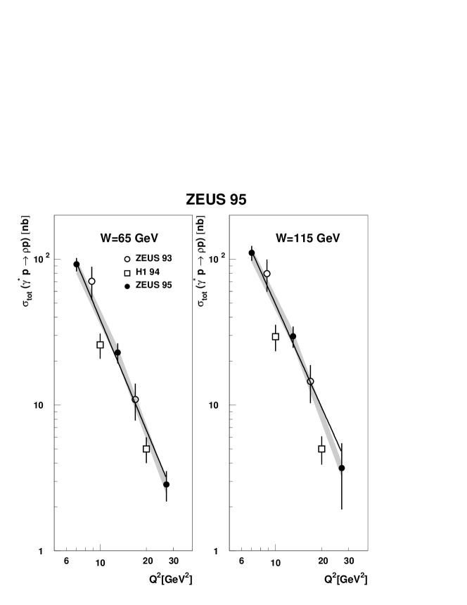
Fig. 115: The dependence of the $\gamma^{*}p\rightarrow\rho^{0}p$ cross section on $Q^{2}$.

Published results exist starting from $Q^{2}=0.25$ GeV² and extending to $Q^{2}=27$ GeV². The cross sections are clearly much smaller than those from photoproduction. This is due to the steep $Q^{2}$ dependence of the cross section, shown graphically in Fig. 115 for $\rho^{0}$ production. Fits of the form $d\sigma/dQ^{2}\propto Q^{-2n}$ to the higher $Q^{2}$ data yield values of $n=2.1-2.5$, while the lower $Q^{2}$ data is well fit by a form of the type $1/(Q^{2}+M_{\rho}^{2})^{2}$. This is more-or-less in line with expectations from both soft exchange and perturbative two-gluon exchange.

$W$ dependence of cross sections

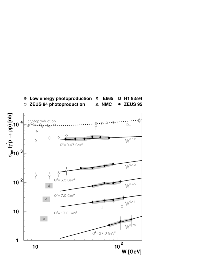
Fig. 116: The cross section for $\gamma^{*}p\rightarrow\rho^{0}p$ as a function of $W$ for different $Q^{2}$ values. The solid lines show the $W$ dependence from fits to ZEUS data. The dashed line is the prediction of ? for photoproduction. The NMC (?), E665 (?) and H1 (?) data were interpolated to the indicated $Q^{2}$ values.

Fig. 117: The cross section for $\gamma^{*}p\rightarrow\phi p$ as a function of $W$ for photoproduction and DIS.

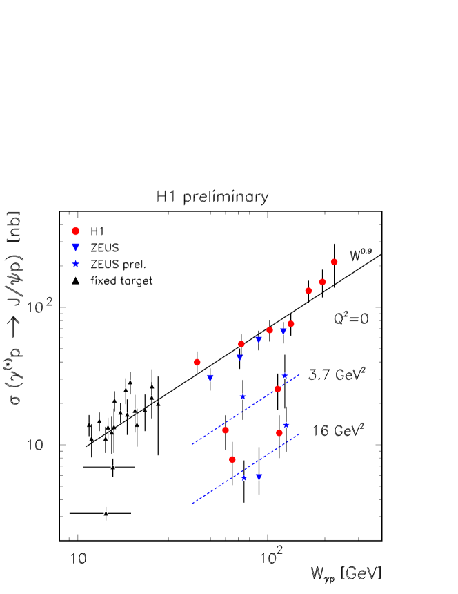
Fig. 118: The cross section for $\gamma^{*}p\rightarrow J/\psi p$ as a function of $W$ for photoproduction and DIS. The lines indicate a $W^{0.9}$ dependence.

The cross section at fixed $Q^{2}$ shows an increase with $W$ when compared to fixed target experiments. This is shown in Fig. 116 for the $\rho^{0}$ meson, in Fig. 117 for the $\phi$ meson, and in Fig. 118 for the $J/\psi$. The ZEUS collaboration has measured the $W$ dependence within its own data  (?) for $\rho^{0}$ electroproduction, and finds

$$\begin{array}[]{llrl}Q^{2}=&0.47~{}\rm{GeV}^{2}&\delta=&0.12\pm 0.03\pm 0.08\;,\\ &3.5&&0.40\pm 0.12\pm 0.12\;,\\ &7.0&&0.45\pm 0.15\pm 0.07\;,\\ &13.0&&0.41\pm 0.19\pm 0.10\;,\\ &27.0&&0.76\pm 0.55\pm 0.60\;.\end{array}$$ (229)

These data are suggestive of an increasing steepness with $W$, but clearly more precision is needed before any conclusion can be drawn. Recent preliminary results for $\rho^{0}$ production from H1 (?) and $\phi$ production from ZEUS (?) show more conclusively the increasing steepness of the $W$ dependence with $Q^{2}$.

The $W$ dependence cannot be measured in the HERA data alone for $J/\psi$ production because of limited statistics. Comparison with the fixed target data indicates that the $\phi$ has a steeper $W$ dependence than the $\rho^{0}$. The same statement applies for the DIS production of $J/\psi$ mesons, where the slope is similar, within errors, to that measured in photoproduction of $J/\psi$.

$t$ slopes versus $Q^{2}$ and $W$

Fig. 119: The slope $b$ of the exponential $t$ dependence $\exp(-b|t|)$ for $\rho^{0}$ production as a function of the photon virtuality $Q^{2}$.

The measurements of the $t$ dependence are summarized in Table 8. The values of $b$ are smaller than those measured in photoproduction, and show a trend to smaller values as $Q^{2}$ increases. This is expected since the contribution to $b$ from the size of the photon should decrease with increasing $Q^{2}$. The $Q^{2}$ dependence of $b$ for $\rho^{0}$ production is shown in Fig. 119. The data are currently not accurate enough to determine whether there is any shrinkage of the forward peak with energy, as expected in Regge Theory.

Tests of SCHC and $R$

The spin density matrix elements have been determined for $\rho^{0}$ production under the hypothesis of SCHC. They indicate that the fraction of $\rho^{0}$ mesons produced in the helicity 0 state increases with $Q^{2}$. If in addition to the SCHC hypothesis, natural parity exchange in the $t$-channel is assumed, then the $r^{1}_{1-1}$ matrix element can be expressed as

$$r^{1}_{1-1}=0.5(1-r^{04}_{00})\;.$$ (230)

The values obtained are consistent with this relationship, indicating that the assumptions of SCHC and natural parity exchange are valid. The transition from helicity $\pm 1$ vector mesons to dominantly helicity $0$ vector mesons as $Q^{2}$ increases is clearly seen in the data. Assuming SCHC, this translates into a strong dependence of $R$ on $Q^{2}$. This dependence is shown in Fig. 120 and compared to different model predictions.

Fig. 120: The ratio $R=\sigma_{L}/\sigma_{T}$ for the reaction $\gamma^{*}p\rightarrow\rho^{0}p$ as a function of $Q^{2}$

Results with proton dissociation

The proton dissociation reaction $ep\rightarrow e\rho^{0}N$, where $N$ is a small mass baryonic system, has also been measured at HERA (?; ?). The $W$, $Q^{2}$ and helicity angle distributions are found to be similar in shape to those measured for the elastic process. However, the $t$ slope is considerably shallower, with measured $b\approx 2$ GeV^-2. These measurements are interesting in their own right, e.g., to test the factorization of the cross section, but are also important for the measurement of the elastic cross section since a fraction of the proton dissociative cross section is indistinguishable from the elastic events in the H1 and ZEUS detectors.

7.4.8 Vector meson production ratios

Fig. 121: Production rate of $\phi$ mesons relative to $\rho^{0}$ as a function of $Q^{2}$. The dashed line corresponds to the ratio $2/9$ expected from the quark charges and a flavor symmetric coupling mechanism.

The measured cross section ratio for $\phi$ relative to $\rho^{0}$ is shown as a function of $Q^{2}$ in Fig. 121. There is a clear tendency for this ratio to increase with $Q^{2}$ to the values expected from a flavor independent production mechanism. This trend has also been observed for $J/\psi$ production.

7.4.9 Comparison with pQCD Models

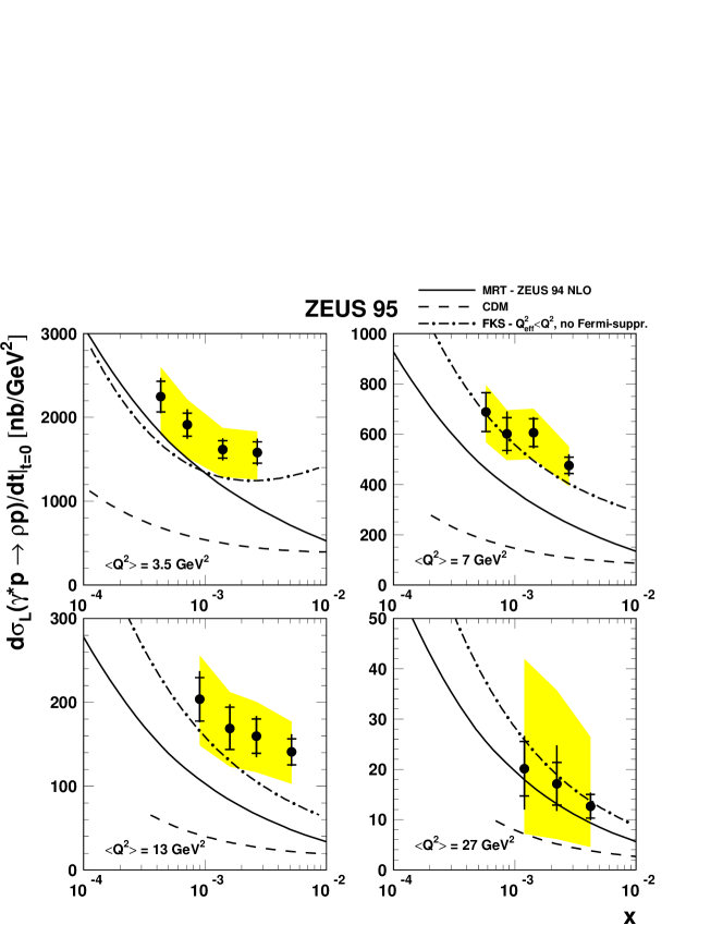
Fig. 122: Comparison of the forward longitudinal cross section, $d\sigma_{L}/d|t||_{t=0}$, to different pQCD models (see text).

The comparison to pQCD calculations is performed for the forward longitudinal cross section, $d\sigma_{L}/d|t||_{t=0}$. The experimental values for $R$ and $b$ must be used to convert the measured $\gamma^{*}p$ cross sections to $d\sigma_{L}/d|t||_{t=0}$. The resulting cross sections tend to have large uncertainties, but nevertheless are able to distinguish between different pQCD models. Figure 122 compares the calculations of the models of ?, ? and Nemchik, Nikolaev, Predazzi and Zakharov (?; ?) to the ZEUS data. The first two models make use of the gluon density extracted by ZEUS from NLO fits to $F_{2}$, and both reproduce the data reasonably well given the remaining large normalization uncertainties. The model of Nemchik et al. underestimates the cross section over the entire kinematic range.

7.5 Discussion

Light vector meson photoproduction shows all the features of soft diffractive scattering: the $W$ dependence is soft, the $t$ dependence is steep, SCHC applies, and the $\rho^{0}$ mass spectrum is skewed. The situation is drastically different for $J/\psi$ production. Here, the $W$ dependence is steep, and the $t$ slope is a factor of two smaller.

As $Q^{2}$ is increased, the light vector mesons become progressively more polarized in the helicity zero state, and the $t$ dependence of the cross section becomes less steep. The situation for the $W$ dependence is not so clear. The data are not precise enough to draw conclusions based on single data sets, and combining data sets is difficult. However, the data indicate a steeper dependence as $Q^{2}$ increases, and the steepness is more pronounced for the heavier vector mesons.

First results exist on vector meson production at large $|t|$ which, in the case of the $J/\psi$, are compatible with pQCD expectations.

In which kinematic regime is the process dominated by perturbative two gluon exchange ? The results show that $J/\psi$ production has a steep $W$ dependence, in accord with pQCD expectations. Assuming that the scale is set by $\mu^{2}=(Q^{2}+m_{J/\psi}^{2}+|t|)/4$, as prescribed in the Ryskin model (?), this would imply that light vector meson production should also be perturbative at $Q^{2}\sim m_{J/\psi}^{2}=10$ GeV². The data for $\rho^{0}$ electroproduction prefer a shallower $W$ dependence at this scale than is observed in $J/\psi$ photoproduction. In addition, there is still a significant contribution from $\sigma_{T}$ ($R=\sigma_{L}/\sigma_{T}\approx 3$) to the $\rho^{0}$ cross section at $Q^{2}=10$ GeV². This implies that this value of the scale is not high enough for light vector mesons production to be fully perturbative in nature, leading to the conclusion that $M_{V}^{2}\;{\rm and}\;Q^{2}$ are not symmetric in the determination of the scale of the reaction.

Vector meson production has proven to be a very interesting process in which to test perturbative QCD. The different scales which enter into the process, $M_{V},\;Q^{2}\;t$, and their interplay, provide a challenge to our understanding of this basic physical process. In pQCD, the cross sections depend on the square of the gluon density, making this process a very interesting one to study the parton densities in the proton. Clearly, further theoretical as well as experimental work is needed. On the theoretical side, higher order calculations are needed to reduce the scale uncertainties and to allow more quantitative predictions. On the experimental side, further extensions in the different scales $Q^{2},\;|t|,\;M$ are needed to understand the transition from soft to hard reactions. This topic will continue to be of interest as it provides a testing ground for pQCD in exclusive reactions.

8 Searches for new particles and new interactions

In the previous sections, we have reported on physics within the realm of the Standard Model (SM) of electroweak+strong interactions. The SM has been exceptionally successful, and there are currently no known violations of its predictions. It is however expected that the SM will not be the final theory, but rather a low energy manifestation of a more general theory, perhaps encompassing gravity. There are many open issues in the Standard Model.

• Why are there three families of quarks and leptons ? In the past, a large number of “fundamental particles” eventually led to a new level substructure (atoms are composed of nuclei and electrons, nuclei are composed of neutrons and protons, hadrons are composed of quarks). It is therefore natural to speculate that new levels of substructure exist within quarks and leptons.

• The mass spectrum of known particles is not understood. In the Standard Model, particles acquire their mass via the mechanism of spontaneous symmetry breaking, leading to the presence of a scalar particle, the Higgs particle. This particle has not yet been observed. Given the observation of the Higgs, the question of the immense gap in mass between the weak bosons, which set the scale of the weak interactions, and the Planck mass, which sets the scale of gravitational interactions, will still need clarification. A theory which explained the observed mass spectrum would be a great step forward in our understanding of nature.

• The SM interactions violate chiral symmetry. This is not currently understood, and theories postulating left-right symmetry at higher energies are certainly tempting to consider.

• Gravity does not appear in the SM. In this context, supersymmetric theories are an exciting possibility since they naturally incorporate gravity. Theories attempting to unify gravity with the strong and electroweak forces have to date not had any experimental verification.

The discovery of new interactions or particles beyond the SM would certainly be welcome as they would lead to new theories and a new conception of nature. There are currently two results from HERA which deviate from Standard Model expectations. These are the observation of excess events at large $x\;{\rm and}\;Q^{2}$, seen by both the H1 (?) and ZEUS (?) collaborations, and the anomalous rate of events with high $p_{T}$ muons and large hadronic $p_{T}$ seen by the H1 collaboration (?). These will be reviewed in some detail below. We also summarize searches which have been carried out for new physics.

The HERA center-of-mass energy, $\sqrt{s}=300$ GeV, is intermediate between those available at LEP (up to about $185$ GeV) and the Tevatron ($1.8$ TeV). The “cleanliness” of the final state is also intermediate between the two since one of the colliding particles is point-like. An advantage of HERA over the Tevatron is that the SM DIS cross sections at high $E_{T}$ can be calculated precisely. Deviations from expectations are therefore more easily spotted.

HERA is of course ideally suited to new states which couple directly to leptons and quarks, such as leptoquarks or some supersymmetric quarks. Searches for excited fermions are also particularly clean, and can be performed up to the kinematic limit.

In the following sections, we review:

• Direct searches for the production of new particles, either as $s$-channel resonances or produced in the $t$-channel. In the direct $s$-channel formation of new particles, the incoming $e^{\pm}$ fuses with a quark or gluon in the proton to form a resonance. Examples of these types of particles are leptoquarks, leptogluons and quarks in R-parity violating supersymmetry. These particles will appear as resonances for $M<\sqrt{s}$. Examples of $t$-channel processes are the single production of excited fermions, heavy neutral leptons or selectron+squark production in R-parity conserving supersymmetry.

• Searches for new interactions at mass scales $\Lambda\stackrel{{\scriptstyle>}}{{\sim}}1$ TeV. These can be studied in the context of 4-fermion contact interactions. In general, the presence of new particles, or compositeness of any kind, are signals for new interactions which in the low energy limit can be described as contact interactions. However, explicit searches for specific types of particles or interactions are more sensitive than the general search for contact interactions, such that the two types of searches are complementary.

• Searches for interactions which violate lepton flavor. Any reaction resulting in flavor violation will be a clear violation of the SM. These searches can be performed in a general way, and can be interpreted as limits on different types of particles appearing in specific models.

• The observation, by the H1 collaboration, of events containing a high $p_{T}$ muon and a hadronic system with large $p_{T}$. The first such event was observed by the H1 collaboration in 1994 (?; ?), and the analysis has since been updated.

• The recent observation of events at large $x,Q^{2}$ observed by the H1 and ZEUS collaborations. First results were presented in February, 1997, and have since been updated.

8.1 Search for leptoquarks and leptogluons

Leptoquarks and leptogluons generally appear in theories which link the leptons and quarks, such as grand unified theories, technicolor models (?), or models for compositeness. Leptoquarks (LQ) are hypothetical color triplet bosons (spin $0$ or $1$), with fractional electric charge, and non-zero lepton and baryon numbers. They couple to lepton-quark pairs, and therefore would appear as s-channel resonances at HERA for $M_{LQ}<\sqrt{s}$. In this case, $M_{LQ}$ is directly related to the fraction of the proton momentum carried by the quark, $x$, as

$$M_{LQ}^{2}=sx\;.$$ (231)

The effects of higher mass leptoquarks can also be observed via a deviation of the observed cross section from SM expectations.

Leptogluons are hypothetical color octet fermions (spin $1/2$) with integer electric charge and non-zero lepton number. They also often appear in theoretical extensions of the SM. Leptogluons would also appear as a resonance in the $x$ distribution if their mass is less than $\sqrt{s}$.

In general, a LQ can couple to multiple lepton and/or quark flavors, thereby providing a mechanism for flavor violation. The different types of leptoquarks with $SU(3)\times SU(2)\times U(1)$ invariant couplings have been worked out by ?. They are distinguished by the quark flavors to which they couple, the lepton flavor to which they couple, their spin, and their chiral properties. Very strong limits exist on chirality violating leptoquarks ($\lambda_{L}\cdot\lambda_{R}>0$, where $\lambda_{L},\;\lambda_{R}$ are the left and right-handed couplings of the LQ), so that we will only consider chirality conserving LQ. Given this constraint, we can distinguish 14 species of LQ, grouped into two sets of 7 species by the fermion number $F=L+3B$, where $L$ and $B$ denote the lepton and baryon number, respectively. These are listed in Table 9. Note that LQ cross sections will be higher for $F=0$ in $e^{+}p$ scattering since in this case a quark fuses with the positron. In $e^{-}p$ scattering, the cross sections are larger for $F=2$.

Table 9: Table showing the different species of leptoquarks and their couplings for those leptoquarks which can be produced at HERA. The leptoquarks in the upper block are color anti-triplets and have fermion number $F=L+3B=0$. The leptoquarks in the lower block are color triplets and have $F=2$. The LQ species are further divided according to their spin ($S$ for scalar and $V$ for vector), their chirality ($L$ or $R$) and their weak isospin ($0,1/2,1$). The leptoquarks ${\tilde{S}}$ and ${\tilde{V}}$ differ by two units of hypercharge from $S$ and $V$, respectively. In addition, the electric charge $q$ of the leptoquarks, the production channel, as well as their allowed decay channels assuming, assuming lepton flavor conservation are displayed. The quantum numbers and decay channels are assuming an electron type LQ. For positrons, the sign of the electric charge is reversed, and anti-quarks should be replaced by the corresponding quark. The nomenclature follows the Aachen convention (?).

LQ species	$q$	Production	Decay	Branching ratio
$S_{1/2}^{L}$	-5/3	$e_{L}\bar{u}_{R}$	$e\bar{u}$	1
$S_{1/2}^{R}$	-5/3	$e_{R}\bar{u}_{L}$	$e\bar{u}$	1
	-2/3	$e_{R}\bar{d}_{R}$	$e\bar{d}$	1
${\tilde{S}}_{1/2}^{L}$	-2/3	$e_{L}\bar{d}_{L}$	$e\bar{d}$	1
$V_{0}^{L}$	-2/3	$e_{L}\bar{d}_{R}$	$e\bar{d}$	1/2
			$\nu_{e}\bar{u}$	1/2
$V_{0}^{R}$	-2/3	$e_{R}\bar{d}_{L}$	$e\bar{d}$	1
${\tilde{V}}_{0}^{R}$	-5/3	$e_{R}\bar{u}_{L}$	$e\bar{u}$	1
$V_{1}^{L}$	-5/3	$e_{L}\bar{u}_{R}$	$e\bar{u}$	1
	-2/3	$e_{L}\bar{d}_{R}$	$e\bar{d}$	1/2
			$\nu_{e}\bar{u}$	1/2
$S_{0}^{L}$	-1/3	$e_{L}{u}_{L}$	$e{u}$	1/2
			$\nu_{e}{d}$	1/2
$S_{0}^{R}$	-1/3	$e_{R}{u}_{R}$	$e{u}$	1
${\tilde{S}}_{0}^{R}$	-4/3	$e_{R}{d}_{R}$	$e{d}$	1
$S_{1}^{L}$	-1/3	$e_{L}{u}_{L}$	$e{u}$	1/2
			$\nu_{e}{d}$	1/2
	-4/3	$e_{L}{d}_{L}$	$e{d}$	1
$V_{1/2}^{L}$	-4/3	$e_{L}{d}_{R}$	$e{d}$	1
$V_{1/2}^{R}$	-4/3	$e_{R}{d}_{L}$	$e{d}$	1
	-1/3	$e_{R}{u}_{L}$	$e{u}$	1
$\tilde{V}_{1/2}^{L}$	-1/3	$e_{L}{u}_{R}$	$e{u}$	1

We can define many possible LQ types (?), depending on the flavors of the quarks and leptons involved in the production and decay. We will initially consider LQ which preserve lepton number, and which couple to a single generation. The more general case involving lepton flavor violation is treated below.

8.1.1 Searches for leptoquarks

Fig. 123: Diagrams showing a) the s-channel production of a leptoquark in $ep$ scattering, and b) the s-channel production of a squark in R-parity violating SUSY, with subsequent decay.

Leptoquarks with masses below $\sqrt{s}$ are formed at HERA via electron (or positron) fusion with a quark or antiquark from the proton. The leading order diagram for this process is shown in Fig. 123.

If the electron-quark coupling is not too large, then the mass of the leptoquark is related to the center-of-mass energy via

$$x_{0}\approx\frac{M_{LQ}^{2}}{s}\;\;.$$ (232)

where $x_{0}$ is the fractional momentum of the proton carried by the quark or anti-quark taking part in the interaction. The width of the leptoquark is given by

$$\Gamma = \frac{\lambda^{2}}{16\pi}M_{LQ}\;\;\;{\rm Spin}\;0\;,$$ (233)

$$= \frac{\lambda^{2}}{24\pi}M_{LQ}\;\;\;{\rm Spin}\;1\;,$$ (234)

where $\lambda$ is the coupling of the LQ to the electron-quark pair. In the narrow width approximation (?), the cross section is given by

$$\sigma(eq\rightarrow LQ) \simeq \frac{\pi}{4s}\lambda^{2}q(x_{0})\;\;\;{\rm Spin}\;0\;,$$ (235)

$$\simeq \frac{2\pi}{4s}\lambda^{2}q(x_{0})\;\;\;{\rm Spin}\;1\;,$$ (236)

where $q$ is the quark (or anti-quark) density in the proton. Note that the quark density is generally evaluated at the scale $\mu=M_{LQ}$.

As can be seen in Table 9, the LQ can either decay to electron+quark, or neutrino+quark. The final states are indistinguishable from normal DIS NC or CC events. The experimental searches for leptoquarks therefore follow the standard neutral current and charged current event selection procedures, and look for enhancements in the $x$ or $M$ distributions, where $M$ is the mass of the electron (neutrino) jet final state. The sensitivity to a leptoquark signal can be enhanced by taking advantage of the $y$ distribution, which differs from that of DIS. A scalar leptoquark, which has an isotropic decay angular distribution in its rest frame, will have a flat $y$ distribution, while vector leptoquarks will have a $(1-y)^{2}$ distribution. To date, no statistically significant signal has been found in these direct searches (see however section 8.7), and 95 % CL limits are set on the size of the allowed lepton-quark coupling as a function of the mass of the leptoquark. The ZEUS limits (?; ?; ?) come from the 1992-3 $e^{-}p$ running (for $F=2$ leptoquarks) and 1994-97 $e^{+}p$ running (for $F=0$ leptoquarks). The limits are based on $0.55$ pb^-1 of $e^{-}p$ data and $47$ pb^-1 of $e^{+}p$ data. H1 has published results based on the 1992-1993 $e^{-}p$ data (?) as well as the 1994 $e^{+}p$ data (?), with luminosities of $0.43$ pb^-1 and $2.83$ pb^-1 respectively. They have also reported limits on scalar leptoquarks from the full 1994-97 $e^{+}p$ data (?). The use of both $e^{-}p$ and $e^{+}p$ data allows strong limits on both $F=0$ and $F=2$ leptoquarks. H1 has additionally set limits on the ratio $M_{LQ}/\lambda$ for $M_{LQ}>\sqrt{s}$ from a contact term analysis (?). The limits achieved by the ZEUS experiment from their 1994-97 data sets are shown in Fig. 124.

Fig. 124: Upper limits from the ZEUS experiment at 95 % CL as a function of mass on the coupling $\lambda$ for scalar and vector leptoquarks which for an $e^{+}$ beam can decay into lepton+$\overline{q}$ (a,b) and lepton+$q$ (c,d). The regions above the curves are excluded. The horizontal lines indicate the approximate coupling for an electroweak scale, $\sqrt{4\pi\alpha}=0.31$.

The mass limits from both experiments on the different leptoquark species are given in Table 10 for a coupling strength equivalent to that of the electroweak interaction, $\lambda=\sqrt{4\pi\alpha}\approx 0.3$. At such a coupling strength, LQ production is ruled out for $M_{LQ}<200$ GeV. The strongest limits are for those LQs which couple to $u$ quarks as these have the largest density at large $x$. For these processes, the limits exceed $280$ GeV. At a fixed mass of $150$ GeV, the limits on $\lambda$ are in many cases below $0.01$.

Table 10: Table showing the mass limits on the different types of leptoquarks for direct as well as indirect searches. For the direct searches, the lower limit on $M_{LQ}$ is given for lepton-quark coupling of electromagnetic strength, $\lambda_{eq_{1}}=\sqrt{4\pi\alpha}$. In the case of indirect searches, the limit is set on $M_{LQ}/\lambda$. The results in column 3 are based on Fig. 2 of reference (?) and, for scalar leptoquarks with $F=2$, on Fig. 11 of reference (?). The results in column 4 are from (?) for $F=2$ leptoquarks, and from Fig. 6 of reference (?) for $F=0$ leptoquarks.

LQ	indirect limit	limit on $M_{LQ}$ (GeV)
species	on $M_{LQ}/\lambda$ (GeV)	for $\lambda=0.31$
	H1	H1	ZEUS
$S_{1/2}^{L}$		275	282
$S_{1/2}^{R}$		275	282
${\tilde{S}}_{1/2}^{L}$	360	263	270
$V_{0}^{L}$		250	268
$V_{0}^{R}$		235	273
${\tilde{V}}_{0}^{R}$	760	260	285
$V_{1}^{L}$	1020	270	287
$S_{0}^{L}$		240	242
$S_{0}^{R}$		245	242
${\tilde{S}}_{0}^{R}$	350	215	214
$S_{1}^{L}$	340	240	245
$V_{1/2}^{L}$	300	220	224
$V_{1/2}^{R}$	710	240	252
$\tilde{V}_{1/2}^{L}$	800	240	251

Other bounds on leptoquarks exist from $e^{+}e^{-}$ scattering, from $p\overline{p}$ scattering, from searches for forbidden decays, and from the observation of lepton universality. In $e^{+}e^{-}$ and $p\overline{p}$ scattering the leptoquarks are produced via electromagnetic or strong interactions which are independent of the lepton-quark coupling strength. The strongest direct limits are from the Tevatron and are currently $213$ GeV from CDF (?) and $225$ GeV from D0 (?). These limits apply to scalar leptoquarks assuming a branching ratio of 1. They depend strongly on the assumed branching ratios of the LQs to electron and neutrinos, with smaller branching ratios giving weaker limits. Weak universality (?; ?) imposes that $\lambda_{L}<M/1.7$ (TeV).

8.1.2 Searches for leptogluons

The leptogluon decay width depends on the ratio $M_{LG}/\Lambda$, where $\Lambda$ is a scale characterizing the underlying interaction, as

$$\Gamma=\frac{\alpha_{s}}{4}\frac{M_{LG}^{3}}{\Lambda^{2}}\;,$$ (237)

where $\alpha_{s}$ is the strong coupling constant. For $M_{LG}\ll\Lambda$, the decay width is small and the total cross section is approximately given by

$$\sigma(eg\rightarrow LG)\simeq\frac{2\pi^{2}\alpha_{s}}{s}(\frac{M_{LG}}{\Lambda})^{2}g(x_{0})\;.$$ (238)

Leptogluons have spin $1/2$, and will therefore have a $y$ distribution of the form $(1-y)$. The analysis proceeds along similar lines to the search for leptoquarks. Leptogluon limits as derived by the H1 collaboration (?) from the 1992 $e^{-}p$ running exclude at 95 % C.L. scale parameters $\Lambda\leq 1.8$ TeV for a leptogluon mass $M=100$ GeV and $\Lambda\leq 200$ GeV at $M=200$ GeV.

8.1.3 Flavor violating interactions

Fig. 125: The (a) $s$-, (b) $u$-, and (c) $t$-channel Feynman diagrams for LFV. For the $s$-channel and $u$-channel diagrams, we denote the couplings as $\lambda_{\ell q}$, where the indices refer to the lepton and quark flavors.

At HERA, lepton flavor violation (LFV) could occur via $s$-, $u$-, or $t$-channel exchanges as shown in Fig. 125. For the $s$- and $u$-channel processes the exchanged particle has the quantum numbers of a leptoquark or an ${\textstyle\not{R}_{P}}$ squark. For the case of $t$-channel exchange, the process would be mediated by a flavor-changing neutral boson. The ZEUS (?) and H1 (?; ?) experiments have performed searches for LFV by looking for events with high $p_{T}$ muons or taus. No evidence for flavor violation was found. This leads to model dependent limits on possible types of leptoquarks or ${\textstyle\not{R}_{P}}$ squarks. We outline the results attained for flavor violating leptoquarks in this section. The results on flavor violation in the context of ${\textstyle\not{R}_{P}}$ squarks are given in section 8.2.2.

We can distinguish 252 different LQ scenarios leading to lepton flavor violation. These are defined by the 14 different LQ species described in Table 9, by the flavors of the quarks which couple to the electron and the final state lepton, and by the final state lepton flavor ($\mu$ or $\tau$). The reactions are described by two dimensionless couplings, $\lambda_{eq_{1}}$ and $\lambda_{lq_{2}}$ defined in Fig. 125. The limit setting procedure depends on whether the search is for LQ with $M_{LQ}<\sqrt{s}$ or $M_{LQ}>\sqrt{s}$.

Fig. 126: The 95 % CL upper limit on the coupling at the decay vertex vs. leptoquark mass $M_{LQ}$, for several values of the first-generation coupling at the production vertex. The dotted curves are for $F=2$ leptoquarks and the solid curves are for $F=0$ leptoquarks.

Fig. 127: The 95 % CL upper limit on the coupling at the decay vertex vs. leptoquark mass $M_{LQ}$, for several values of the first-generation coupling at the production vertex. The dotted curves are for $F=2$ leptoquarks and the solid curves are for $F=0$ leptoquarks.

• For $M_{LQ}<\sqrt{s}$, limits can be set on $M_{LQ}$ for given coupling strengths $\lambda_{eq_{1}},\lambda_{lq_{2}}$ or $\lambda_{eq_{1}}$ and branching ratio $B(lq_{2})=\lambda_{lq_{2}}^{2}/(\lambda_{eq_{1}}^{2}+\lambda_{lq_{2}}^{2})$. Limits on $\lambda_{lq_{2}}$ versus $M_{LQ}$ are shown for fixed values of $\lambda_{eq_{1}}$ in Fig. 126 for the ZEUS analysis, and Fig. 127 for the H1 analysis. For this figure, only leptoquarks with no neutrino decay modes are shown, and it is assumed that the branching ratio for the decay $LQ\rightarrow l+q_{2}$ is given by $B_{lq_{2}}=\lambda_{lq_{2}}^{2}/(\lambda_{eq_{1}}^{2}+\lambda_{lq_{2}}^{2})$. For flavor violating couplings of electromagnetic strength, the ZEUS collaboration sets 95 % CL lower limits on leptoquark masses between $207$ GeV and $272$ GeV, depending on the LQ species and final-state lepton. The recent H1 results (?) extend the limits further. For $\lambda_{eq_{1}}=\lambda_{\tau q_{2}}=0.03$, the excluded mass range is extended by about $65$ GeV.

• For $M_{LQ}>\sqrt{s}$, the cross section is proportional to the square of $\lambda_{eq_{1}}\lambda_{lq_{2}}/M_{LQ}^{2}$, and ZEUS has set upper bounds on this quantity. Many of the ZEUS limits supersede prior limits (?), particularly in the case where $e\rightarrow\tau$. The results for this case are summarized in Tables 11 and 12.

Table 11: The best upper bounds on $\lambda_{eq_{1}}\lambda_{\tau q_{2}}/M_{LQ}^{2}$ for $F=0$ leptoquarks, in units of $10^{-4}$ GeV^-2. Each column corresponds to a given leptoquark species and each row to the quark flavors $q_{1}$ and $q_{2}$ which couple to $e$ and $\tau$, the generation indices of which are specified in the first column. The possible decay models of the LQ are listed, including decays not possible at HERA but possible at other experiments. The top line in each box gives the previous measurement (?) which had obtained the strictest limit. The limit from that experiment is given on the second line in the box and the ZEUS limit, shown on the third line, is printed in boldface if it supersedes the previous limit. The asterisks denote those cases where lepton flavor violation occurs only via processes involving top.

$e\leftrightarrow\tau$                                   $F=0$
	$S_{1/2}^{L}$	$S_{1/2}^{R}$	$\tilde{S}_{1/2}^{L}$	$V_{0}^{L}$	$V_{0}^{R}$	$\tilde{V}_{0}^{R}$	$V_{1}^{L}$
$(q_{1}q_{2})$	$e^{-}\bar{u}$	$e^{-}(\bar{u}+\bar{d})$	$e^{-}\bar{d}$	$e^{-}\bar{d}$	$e^{-}\bar{d}$	$e^{-}\bar{u}$	$e^{-}(\sqrt{2}\bar{u}+\bar{d})$
	$\nu\;\,\bar{u}$		$\nu\;\,\bar{d}$	$\nu\;\,\bar{u}$			$\nu\;\,(\bar{u}+\sqrt{2}\bar{d})$
(11)	$\tau\rightarrow\pi e$	$\tau\rightarrow\pi e$	$\tau\rightarrow\pi e$	$G_{F}$	$\tau\rightarrow\pi e$	$\tau\rightarrow\pi e$	$G_{F}$
	0.02	0.01	0.02	0.002	0.01	0.01	0.002
	0.11	0.09	0.18	0.11	0.11	0.07	0.04
(12)		$\tau\rightarrow Ke$	$K\rightarrow\pi\bar{\nu}\nu$	$\tau\rightarrow Ke$	$\tau\rightarrow Ke$		$K\rightarrow\pi\bar{\nu}\nu$
		0.05	$2\times 10^{-5}$	0.03	0.03		$5\times 10^{-6}$
	0.12	0.10	0.18	0.15	0.15	0.10	0.05
(13)		$B\rightarrow\tau\bar{e}X$	$B\rightarrow\tau\bar{e}X$	$B\rightarrow\ell\nu X$	$B\rightarrow\tau\bar{e}X$		$B\rightarrow\ell\nu X$
		0.08	0.08	0.02	0.04		0.02
	*	0.18	0.18	0.16	0.16	*	0.16
(21)		$\tau\rightarrow Ke$	$K\rightarrow\pi\bar{\nu}\nu$	$\tau\rightarrow Ke$	$\tau\rightarrow Ke$		$K\rightarrow\pi\bar{\nu}\nu$
		0.05	$2\times 10^{-5}$	0.03	0.03		$5\times 10^{-6}$
	0.34	0.26	0.39	0.14	0.14	0.10	0.05
(22)	$\tau\rightarrow e\gamma$	$\tau\rightarrow e\gamma$
	0.2	0.2
	0.60	0.37	0.48	0.25	0.25	0.31	0.13
(23)		$B\rightarrow\tau\bar{e}X$	$B\rightarrow\tau\bar{e}X$	$B\rightarrow\ell\nu X$	$B\rightarrow\tau\bar{e}X$		$B\rightarrow\ell\nu X$
		0.08	0.08	0.02	0.04		0.02
	*	0.50	0.50	0.33	0.33	*	0.33
(31)		$B\rightarrow\tau\bar{e}X$	$B\rightarrow\tau\bar{e}X$	$V_{bu}$	$B\rightarrow\tau\bar{e}X$		$V_{bu}$
		0.08	0.08	0.002	0.04		0.002
	*	0.47	0.47	0.15	0.15	*	0.15
(32)		$B\rightarrow\tau\bar{e}X$	$B\rightarrow\tau\bar{e}X$	$B\rightarrow\ell\nu X$	$B\rightarrow\tau\bar{e}X$		$B\rightarrow\ell\nu X$
		0.08	0.08	0.02	0.04		0.02
	*	0.65	0.65	0.26	0.26	*	0.26
(33)				$\tau\rightarrow e\gamma$	$\tau\rightarrow e\gamma$
				3.4	3.4
	*	0.72	0.72	0.38	0.38	*	0.38

Table 12: The best upper bounds on $\lambda_{eq_{1}}\lambda_{\tau q_{2}}/M_{\scriptscriptstyle LQ}^{2}$ for $F=2$ leptoquarks, in units of $10^{-4}$ GeV^-2. Each column corresponds to a given leptoquark species and each row to the quark flavors $q_{1}$ and $q_{2}$ which couple to $e$ and $\tau$, the generation indices of which are specified in the first column. The top line in each box gives the previous measurement (?) which had obtained the strictest limit. The limit from that experiment is given on the second line in the box and the ZEUS limit, shown on the third line, is printed in boldface if it supersedes the previous limit. The asterisks denote those cases where lepton flavor violation occurs only via processes involving top.

$e\leftrightarrow\tau$                                   $F=2$
	$S_{0}^{L}$	$S_{0}^{R}$	$\tilde{S}_{0}^{R}$	$S_{1}^{L}$	$V_{1/2}^{L}$	$V_{1/2}^{R}$	$\tilde{V}_{1/2}^{L}$
$(q_{1}q_{2})$	$e^{-}u$	$e^{-}u$	$e^{-}d$	$e^{-}(u+\sqrt{2}d)$	$e^{-}d$	$e^{-}(u+d)$	$e^{-}u$
	$\nu\;\,d$			$\nu\;\,(\sqrt{2}u+d)$	$\nu\;\,d$		$\nu\;\,u$
(11)	$G_{F}$	$\tau\rightarrow\pi e$	$\tau\rightarrow\pi e$	$G_{F}$	$\tau\rightarrow\pi e$	$\tau\rightarrow\pi e$	$\tau\rightarrow\pi e$
	0.003	0.02	0.02	0.003	0.01	0.005	0.01
	0.15	0.15	0.23	0.09	0.09	0.05	0.06
(12)	$K\rightarrow\pi\bar{\nu}\nu$		$\tau\rightarrow Ke$	$K\rightarrow\pi\bar{\nu}\nu$	$K\rightarrow\pi\bar{\nu}\nu$	$\tau\rightarrow Ke$
	$2\times 10^{-5}$		0.05	$2\times 10^{-5}$	$10^{-5}$	0.03
	0.20	0.20	0.27	0.11	0.19	0.13	0.16
(13)	$V_{bu}$		$B\rightarrow\tau\bar{e}X$	$V_{bu}$	$B\rightarrow\tau\bar{e}X$	$B\rightarrow\tau\bar{e}X$
	0.004		0.08	0.004	0.04	0.04
		*	0.28	0.14	0.23	0.23	*
(21)	$K\rightarrow\pi\bar{\nu}\nu$		$\tau\rightarrow Ke$	$K\rightarrow\pi\bar{\nu}\nu$	$K\rightarrow\pi\bar{\nu}\nu$	$\tau\rightarrow Ke$
	$2\times 10^{-5}$		0.05	$2\times 10^{-5}$	$10^{-5}$	0.03
	0.22	0.22	0.31	0.12	0.09	0.05	0.06
(22)	$\tau\rightarrow e\gamma$	$\tau\rightarrow e\gamma$	$\tau\rightarrow e\gamma$	$\tau\rightarrow e\gamma$
	0.5	0.5	0.3	0.1
	0.60	0.60	0.48	0.22	0.25	0.19	0.31
(23)	$B\rightarrow\ell\nu X$		$B\rightarrow\tau\bar{e}X$	$B\rightarrow\ell\nu X$	$B\rightarrow\tau\bar{e}X$	$B\rightarrow\tau\bar{e}X$
	0.04		0.08	0.04	0.04	0.04
		*	0.50	0.25	0.33	0.33	*
(31)	$B\rightarrow\ell\nu X$		$B\rightarrow\tau\bar{e}X$	$B\rightarrow\ell\nu X$	$B\rightarrow\tau\bar{e}X$	$B\rightarrow\tau\bar{e}X$
	0.04		0.08	0.04	0.04	0.04
		*	0.34	0.17	0.10	0.10	*
(32)	$B\rightarrow\ell\nu X$		$B\rightarrow\tau\bar{e}X$	$B\rightarrow\ell\nu X$	$B\rightarrow\tau\bar{e}X$	$B\rightarrow\tau\bar{e}X$
	0.04		0.08	0.04	0.04	0.04
		*	0.65	0.32	0.26	0.26	*
(33)			$\tau\rightarrow e\gamma$	$\tau\rightarrow e\gamma$
			0.3	0.1
		*	0.72	0.36	0.38	0.38	*

8.2 Supersymmetry at HERA

Supersymmetry (SUSY) (?; ?) is widely acknowledged as a leading candidate theory to describe possible physics not included in the Standard Model. It relates the properties of fermions to those of bosons (e.g., in SUSY, selectrons, $\widetilde{e}$ are scalar partners of electrons, $e$) and locally supersymmetric theories naturally incorporate gravity. SUSY also resolves in a natural way, in the unbroken version, the hierarchy (or naturalness) problem; i.e., why the ratio $M_{W}/M_{Planck}$ is so small. It is therefore of great interest to search for signs of this new theory. To date, no evidence for supersymmetry has been found.

The fact that the superpartners to the existing particles have not been observed implies that supersymmetry is broken. The breaking of supersymmetry introduces many new parameters into the theory which makes the classification of possible SUSY scenarios rather forbidding. In general, assumptions must be made to reduce the number of parameters and thereby allow for reasonably compact classification schemes (?). In the sections which follow, we will only consider the minimal supersymmetric model (MSSM) and $R$-parity violating supersymmetry.

8.2.1 The minimal supersymmetric model - MSSM

The simplest supersymmetric extension of the Standard Model is denoted MSSM (for minimal supersymmetric model). It is a direct generalization of the Standard Model, with electroweak symmetry breaking occurring via vacuum expectation values of two different Higgs superfields, denoted $H^{1}$ and $H^{2}$. Baryon number and lepton number are separately conserved. This is most easily expressed in terms of the multiplicative quantum number $R$-parity, defined as $R_{P}=(-1)^{3B+L+2S}$ where $B$ is the baryon number, $L$ is the lepton number and $S$ the spin of the particle, so that $R_{P}=+1$ for SM particles and $R_{P}=-1$ for SUSY particles. The MSSM contains the smallest number of new particles and new interactions compatible with the Standard Model. If $R$-parity were conserved, SUSY particles would be produced in pairs and would ultimately decay into the lightest supersymmetric particle (LSP), which would be stable and neutral. It is therefore expected in MSSM that signatures with missing energy would arise since the LSP would escape the detector unseen.

The spectrum of particles expected in the MSSM, in addition to those already known in the SM, includes scalar squarks and sleptons, spin-$1/2$ charginos, neutralinos, the gluino and five different Higgs bosons. Charginos and neutralinos are charged and neutral mass eigenstates of the (mixed) supersymmetric partners of the $W^{\pm},Z^{0},\gamma$ (gauginos) and the two Higgs doublets (higgsinos). The LSP is constrained to be neutral for cosmological reasons, and it is therefore generally assumed that the lightest neutralino, $\chi_{1}^{0}$, is the LSP. There are in addition many possible couplings. The MSSM therefore contains many new parameters and further assumptions are necessary to reduce these to a more tractable number. This necessarily introduces model dependence in the interpretation of searches for new particles. A common approach is to use constraints from supergravity models (?) to express the various SUSY parameters in terms of a common scalar mass $m_{0}$, a common gaugino mass $m_{1/2}$, the ratio of the vacuum expectation value of the two Higgs superfields $\tan\beta$, a common trilinear interaction $A_{0}$, and a sign parameter $sign(\mu)$.

Fig. 128: Feynman diagram for selectron-squark production via neutralino exchange and the subsequent decays into the lightest supersymmetric particle $\chi_{1}^{0}$.

The dominant MSSM process expected at HERA is the production of a selectron and a squark via neutralino exchange, $ep\rightarrow\widetilde{e}\widetilde{q}X$, depicted in Fig. 128. The H1 and ZEUS collaborations have performed searches for this channel (?; ?). The selectron and squark are taken to decay into the lightest neutralino plus SM particles, and the appropriate branching ratios are used. The limits are found under the following assumptions:

• $M_{{\widetilde{e}}_{L}}=M_{{\widetilde{e}}_{R}}$;

• $M_{{\widetilde{q}}_{L}}=M_{{\widetilde{q}}_{R}}$;

• the four lightest squarks are assumed to be mass degenerate;

• the GUT relation $M_{1}=5/3M_{2}\tan^{2}\theta_{W}$ holds.

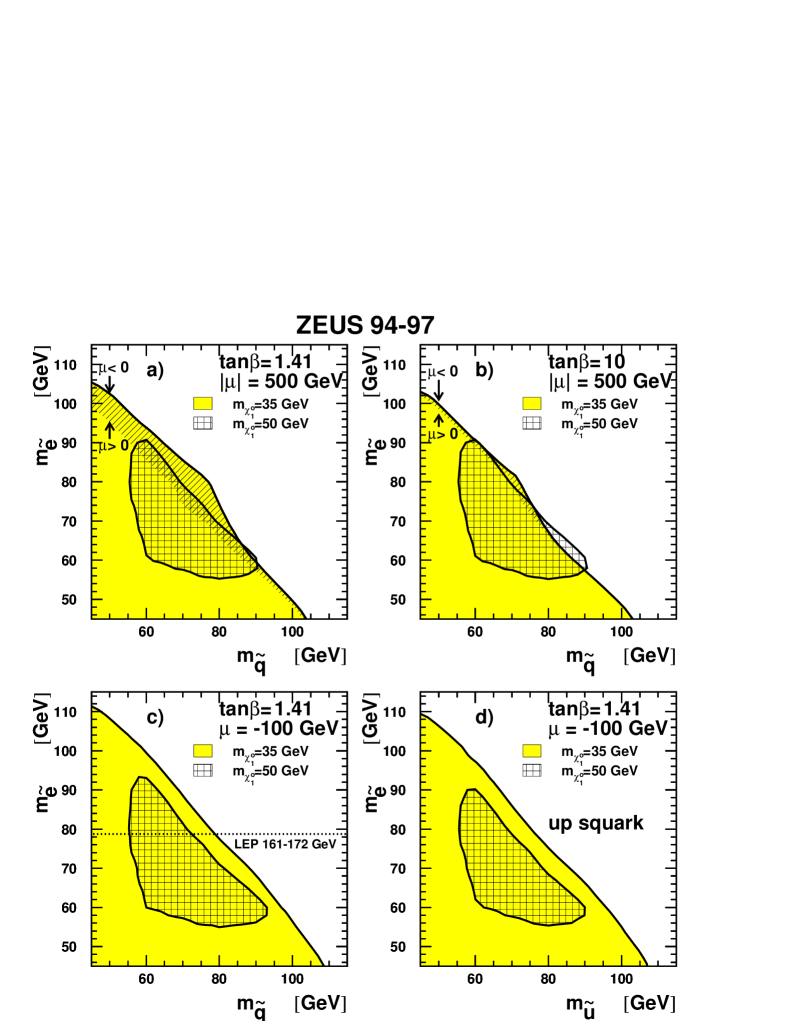
Fig. 129: Excluded region at 95 % CL in the plane defined by the selectron and the squark mass, for two different values of the neutralino mass, $m_{\chi_{1}^{0}}=35,50$ GeV. In a) and b) the limits are for $|\mu|=500$ GeV and $\tan\beta=1.41,10$. For $\mu<0$, the excluded region also includes the single-hatched area. The limits obtained for $\mu=-100$ GeV and $\tan\beta=1.41$ are shown in c) along with the LEP limits on $m_{\tilde{e}}$. The limits for the up squark alone are shown in d).

An integrated luminosity of $6.38$ pb^-1 of $e^{+}p$ collisions was used in the H1 search and $47$ pb^-1 for the ZEUS search, and signatures based principally on missing energy and missing transverse momentum were searched for. For $\tan\beta=\sqrt{2}$, masses below $(M_{\widetilde{e}}+M_{\widetilde{q}})/2=77$ GeV for $M_{\chi^{0}_{1}}=40$ GeV are excluded at $95$ % confidence level. The limits are compared to contemporaneous LEP results (?; ?; ?) in Fig. 129. The HERA results exceed beyond the LEP results for squark masses below about $80$ GeV. LEP experiments (?; ?; ?) have also reported limits on stop and on sbottom of about $75$ GeV. The limits from HERA, for $M_{\widetilde{e}}=M_{\widetilde{q}}$ are at the same level. Since the production at HERA is principally off up quarks, the HERA limits on $(M_{\widetilde{e}}+M_{\widetilde{u}})/2>75$ GeV are almost as high as considering all squarks.

Strong limits on the squark mass have been obtained at the Tevatron (?; ?) which are complementary to those obtained at HERA. The Tevatron squark limits are in general at several hundred GeV. However, they are obtained using GUT inspired assumptions not required by the HERA experiments and they are less sensitive for small mass differences $M_{\widetilde{q}}-M_{\chi_{1}^{0}}$. The HERA analyses probe different regions of MSSM parameter space where the gluinos are heavier than the squarks and the squark masses are independent of the selectron mass.

8.2.2 R parity violating SUSY

$R$-parity need not be conserved in supersymmetric theories. The general superpotential allows for Yukawa couplings between the Standard Model fermions and ${\tilde{q}}$ or ${\tilde{l}}$. However, superpotential terms which violate $R$-parity can in some cases lead to proton decay, which has very stringent experimental constraints, so that the appropriate couplings must be small. Of particular interest for $ep$ collisions are $R$-parity violating superpotential terms of the form $\lambda^{\prime}_{ijk}L^{i}_{L}Q^{j}_{L}{\overline{D}}^{k}_{R}$ (?). Here $L_{L}$, $Q_{L}$, and ${\overline{D}}_{R}$ denote left-handed lepton and quark doublets and the right handed $d$-quark singlet chiral superfields respectively, and the indices $i$, $j$, and $k$ label their respective generations. Expanded into four-component Dirac notation, the corresponding terms of the Lagrangian are

$${\cal L} = \lambda^{\prime}_{ijk}\left[{\tilde{\nu}}^{i}_{L}{\overline{d}}^{k}_{R}d^{j}_{L}+{\tilde{d}}^{j}_{L}{\overline{d}}^{k}_{R}\nu^{i}_{L}+({\tilde{d}}^{k}_{R})^{*}({\overline{\nu}}^{i}_{L})^{c}d^{j}_{L}\right.$$ (239)

$$\mbox{ }-\left.{\tilde{e}}^{i}_{L}{\overline{d}}^{k}_{R}u^{j}_{L}-{\tilde{u}}^{j}_{L}{\overline{d}}^{k}_{R}e^{i}_{L}-({\tilde{d}}^{k}_{R})^{*}({\overline{e}}^{i}_{L})^{c}u^{j}_{L}\right]+{\rm h.~{}c.}$$

Table 13: Table showing the different single squark production processes via an ${\textstyle\not{R}_{P}}$ coupling at HERA with an $e^{+}$ beam.

$\lambda_{1jk}^{\prime}$	Production process
	down type squarks	up type squarks
$111$	$e^{+}+\bar{u}\rightarrow\bar{{\tilde{d}}}_{R}$	$e^{+}+d\rightarrow{\tilde{u}}_{L}$
$112$	$e^{+}+\bar{u}\rightarrow\bar{{\tilde{s}}}_{R}$	$e^{+}+s\rightarrow{\tilde{u}}_{L}$
$113$	$e^{+}+\bar{u}\rightarrow\bar{{\tilde{b}}}_{R}$	$e^{+}+b\rightarrow{\tilde{u}}_{L}$
$121$	$e^{+}+\bar{c}\rightarrow\bar{{\tilde{d}}}_{R}$	$e^{+}+d\rightarrow{\tilde{c}}_{L}$
$122$	$e^{+}+\bar{c}\rightarrow\bar{{\tilde{s}}}_{R}$	$e^{+}+s\rightarrow{\tilde{c}}_{L}$
$123$	$e^{+}+\bar{c}\rightarrow\bar{{\tilde{b}}}_{R}$	$e^{+}+b\rightarrow{\tilde{c}}_{L}$
$131$	$e^{+}+\bar{t}\rightarrow\bar{{\tilde{d}}}_{R}$	$e^{+}+d\rightarrow{\tilde{t}}_{L}$
$132$	$e^{+}+\bar{t}\rightarrow\bar{{\tilde{s}}}_{R}$	$e^{+}+s\rightarrow{\tilde{t}}_{L}$
$133$	$e^{+}+\bar{t}\rightarrow\bar{{\tilde{b}}}_{R}$	$e^{+}+b\rightarrow{\tilde{t}}_{L}$

Table 14: 95% CL mass limits (GeV) from ZEUS for squarks with ${\textstyle\not{R}_{P}}$-couplings, of electromagnetic strength ($\lambda_{11k}^{2}=\lambda_{ijk}^{2}=4\pi\alpha=4\pi/128$), for different masses of the lightest SUSY particle (LSP), denoted $\chi_{1}^{0}$. The mixing angle of the stop is assumed to be $\cos^{2}\theta_{t}=0.5$. The limits for the $m_{\chi_{1}^{0}}=0$ case are somewhat weaker than those for a heavy LSP because ZEUS did not search for the gauge decay ${\tilde{q}}\to q\chi_{1}^{0}$.

	${\tilde{d}}\rightarrow\mu q$	${\tilde{u}}\rightarrow\mu q$	${\tilde{t}}\rightarrow\mu q$	${\tilde{d}}\rightarrow\tau q$	${\tilde{u}}\rightarrow\tau q$	${\tilde{t}}\rightarrow\tau q$
$m_{\chi_{1}^{0}}=0$	229	229	-	221	222	-
$m_{\chi_{1}^{0}}+m_{q}\geq m_{\tilde{q}}$	231	234	223	223	228	216

For $i=1$, which is the case at HERA, the last two terms will result in ${\tilde{u}}$ and ${\tilde{d}}$ type squark production in $ep$ collisions. All possible right-handed down type squarks and left-handed up type squarks can be produced, as listed in Table 13. In $e^{+}p$ collisions these are produced off up type antiquarks and down type quarks, respectively. There are thus 18 possible production couplings probed in $e^{+}p$ collisions. For production and decay via $\lambda^{\prime}_{ijk}$, the squarks behave as scalar leptoquarks and the final state will be indistinguishable, event-by-event, from Standard Model neutral and charged current events. However, as with the scalar leptoquarks, the angular distributions of the final state lepton and quark will be different and this fact can be exploited in performing searches.

Fig. 130: Lowest order $s$-channel diagrams for first generation squark production via $e^{+}d$ scattering at HERA followed by (a) ${\textstyle\not{R}_{P}}$ decay and (b) gauge decay. In (b), the emerging neutralino or chargino might subsequently undergo ${\textstyle\not{R}_{P}}$ decays of which an examples is shown in the dotted box for the $\chi_{1}^{+}$.

In addition to the Yukawa couplings, there are also gauge couplings such that the ${\tilde{q}}$ can decay by radiating a neutralino or chargino. The neutralino or chargino can then subsequently decay. The final state signature will depend on the properties of the neutralino or chargino involved. Figure 130 shows examples of both Yukawa type decays and gauge type decays. For the gauge decays, examples are given of subsequent decays of the neutralino or chargino. The H1 collaboration has searched for ${\textstyle\not{R}_{P}}$ squark production (?; ?) under the following assumptions:

• One $\lambda^{\prime}_{ijk}$ dominates;

• $M_{\widetilde{q_{R}}}\approx M_{\widetilde{q_{L}}}$ for the first two generations;

• The lightest neutralino, $\chi_{1}^{0}$, is the lightest SUSY particle;

• $M_{\widetilde{g}}>M_{\widetilde{q}}$.

The stop is a special case since it is not ruled out that it can be lighter than the corresponding Standard Model particle, the top quark.

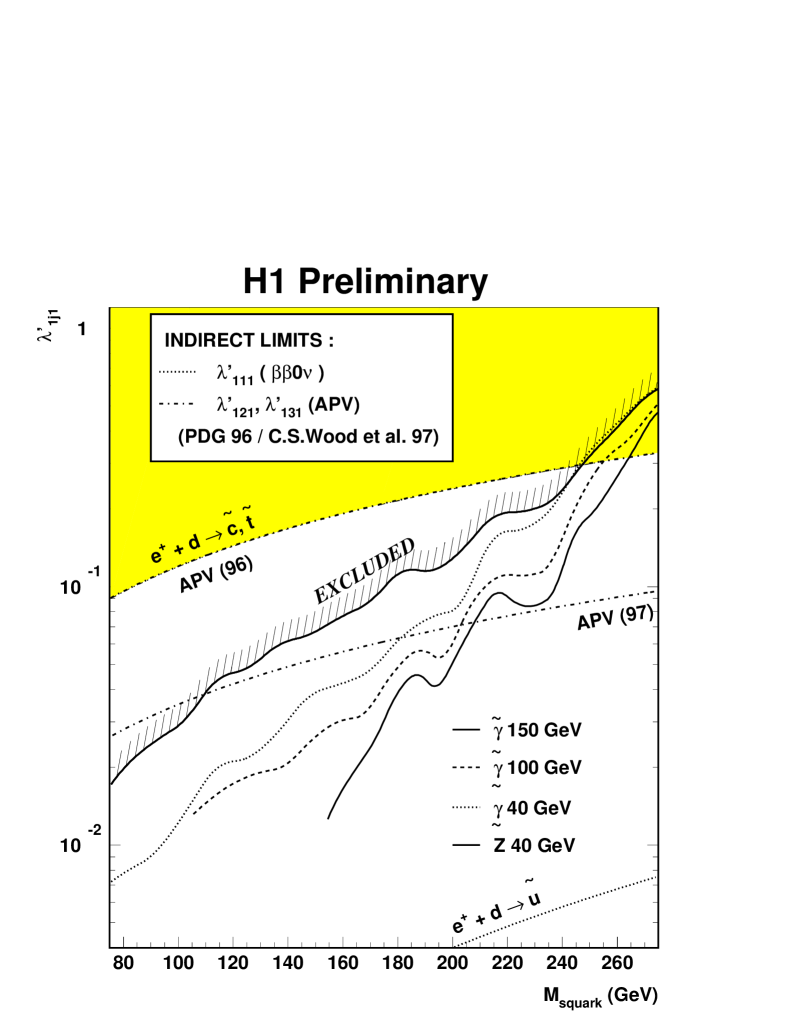
Fig. 131: Exclusion upper limits at 95 % CL for the coupling $\lambda_{1j1}^{\prime}$ as a function of the squark mass for various masses and mixtures of the $\chi_{1}^{0}$; also represented are the most stringent indirect limits on $\lambda_{111}^{\prime}$ and $\lambda_{1j1}^{\prime},j=2,3$.

A systematic analysis of the possible final states resulting from the different production and decay modes was performed, and the search procedure was optimized for each. No significant evidence for SUSY particle production was found, and the H1 collaboration excludes ${\tilde{u}}$ and ${\tilde{d}}$ under various model assumptions. In Fig. 131, exclusion limits on $\lambda_{1j1}^{\prime}$ are shown as a function of the squark mass for different assumptions on the $\chi_{1}^{0}$ mass and composition. Under these conditions, squarks up to masses of $262$ GeV are ruled out at $95$ % CL for $\lambda_{1j1}^{{}^{\prime}2}=4\pi\alpha$.

The Tevatron leptoquark limits rule out ${\tilde{u}}_{L}^{j}$ squark masses below $200$ GeV for branching fractions into $e^{+}q$ greater than 50 %. However, the limits degrade quickly as the branching lower becomes smaller, which is a natural feature in R-parity violating SUSY.

The indirect limits from atomic parity violation (?) and from the non-observation of neutrinoless double beta decay (?; ?) are compared to the HERA limits in Fig. 131. The most stringent limits come from the neutrinoless double beta decay searches but only concern the $\lambda^{\prime}_{111}$ coupling. For the couplings $\lambda^{\prime}_{121},\lambda^{\prime}_{131}$ the limits are comparable to the HERA results.

8.2.3 R-parity violation and lepton flavor violation

Fig. 132: $R_{P}$ violating single squark production in $ep$ collisions. Diagrams a) and b) show production of ${\tilde{u}}$ and ${\tilde{d}}$ squarks with leptoquark-like ${\textstyle\not{R}_{P}}$ decays, where $\ell^{i}$ denotes the final-state charged lepton of generation $i$. The indices $j$ and $k$ denote the generations of up-type and down-type (s)quarks respectively. Diagram c) shows ${\tilde{u}}$ production with an $R_{P}$-conserving decay.

Lepton-flavor violating $ep$ interactions would occur in a model with two non-zero couplings $\lambda^{\prime}_{ijk}$ which involve different lepton generations. For example, the process $e^{+}d\to{\tilde{u}}^{j}\to\mu^{+}d^{k}$ involves the couplings $\lambda^{\prime}_{1j1}$ and $\lambda^{\prime}_{2jk}$. Similarly, non-zero values for $\lambda^{\prime}_{11k}$ and $\lambda^{\prime}_{3jk}$ would lead to the reaction $e^{-}u\to{\tilde{d}}^{k}\to\tau^{-}u^{j}$ (see Fig. 132). Down-type squarks have the additional decay ${\tilde{d}}^{k}\to\nu^{i}d^{j}$, a mode unavailable to up-type squarks.

As pointed out above, the difference between mechanisms involving $R$-parity violating squarks and leptoquarks is that the squarks have the additional decay mode ${\tilde{q}}\to q\chi_{1}^{0}$ shown in Fig. 130. The branching ratios $B_{q\chi_{1}^{0}}$ for the $R_{P}$-conserving decay ${\tilde{q}}\to q\chi_{1}^{0}$ and $B_{ijk}^{\prime}$ for any ${\textstyle\not{R}_{P}}$ decay mode are related (?) by

$${{B_{ijk}^{\prime}}\over{(\lambda_{ijk}^{\prime})^{2}}}={{B_{q\chi_{1}^{0}}}\over{8\pi\alpha}e_{{\tilde{q}}}^{2}(1-{m_{\chi_{1}^{0}}^{2}}/{m_{{\tilde{q}}}^{2})^{2}}},$$ (240)

where $\lambda_{ijk}^{\prime}$ is the ${\textstyle\not{R}_{P}}$ coupling at the decay vertex, $\alpha$ is the electromagnetic coupling, $e_{\tilde{q}}$ is the squark charge in units of the electron charge and the LSP and squark masses are $m_{\chi_{1}^{0}}$ and $m_{\tilde{q}}$, respectively.

Coupling limits for LFV decays of an $S_{0}^{L}$ leptoquark can be interpreted as ${\tilde{d}}^{k}$ coupling limits through the correspondence $\lambda_{eq_{1}}\sqrt{B_{\ell q_{2}}}=\lambda_{11k}^{\prime}\sqrt{B_{ijk}^{\prime}}$ where $i$ and $j$ are the generations of the LQ decay products $\ell$ and $q_{2}$. Similarly, coupling limits on the $\tilde{S}_{1/2}^{L}$ LQ can be converted to limits on couplings to ${\tilde{u}}^{j}$ via $\lambda_{eq_{1}}\sqrt{B_{\ell q_{2}}}=\lambda_{1j1}^{\prime}\sqrt{B_{ijk}^{\prime}}$, where $i$ and $k$ are the generations of $\ell$ and $q_{2}$.

If the stop (${\tilde{t}}$) (?) is lighter than the top quark, then the $R_{P}$-conserving decay ${\tilde{t}}\rightarrow t\chi_{1}^{0}$ will not exist. In the case of ${\tilde{t}}$, the correspondence with the coupling limit on $\tilde{S}_{1/2}^{L}$ is given by $\lambda_{ed}\sqrt{B_{\ell q_{2}}}=\cos\theta_{t}\lambda_{131}^{\prime}\sqrt{B_{i3k}^{\prime}}$ where $\theta_{t}$ is the mixing angle between the SUSY partners of the left- and right-handed top quarks. Over a broad range of possible stop masses, it is expected that $\cos^{2}\theta_{t}\sim 0.5$ (?).

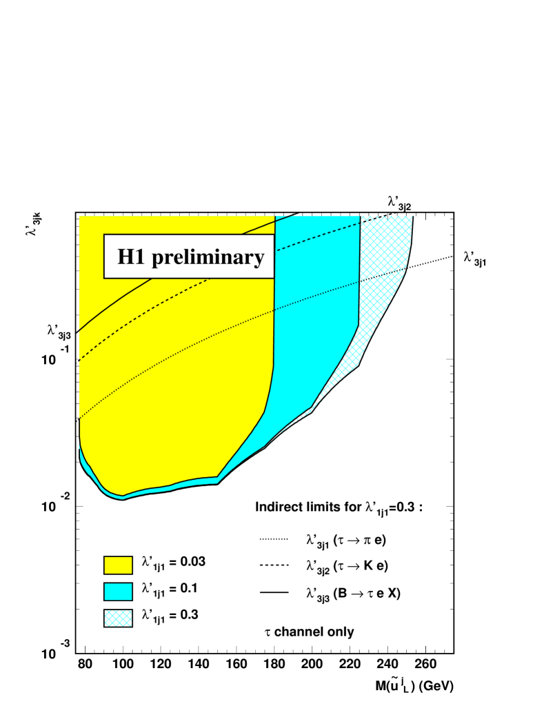
Fig. 133: Upper limits at the 95 % CL for the coupling $\lambda_{3jk}^{\prime}$ as a function of squark mass for different values of $\lambda_{1j1}^{\prime}$. The best indirect limits are also shown.

The ZEUS (?) and H1 (?) collaborations have set limits on ${\textstyle\not{R}_{P}}$-squarks leading to LFV. Table 14 gives the lower limits from the ZEUS experiment for ${\tilde{d}}$, ${\tilde{u}}$ and ${\tilde{t}}$ quarks assuming that the couplings at the production and decay vertex are equal to the electromagnetic coupling. The H1 collaboration has set limits on $\lambda_{3jk}$ assuming different values for $\lambda_{1j1}$, and assuming that gauge decays of squarks are forbidden. These limits are shown in Fig. 133. The limits from indirect searches (?) are also given in the figure, and are seen to be substantially weaker. The Tevatron limits, resulting from searches for $\tau\tau bb$ final states (?) and for $\nu\nu bb$ final states (?) extend to about $99$ GeV. The mass limits from HERA are substantially better than those achieved by previous experiments, particularly in the case where the $\tau$ is involved

8.3 Search for excited fermions

Fig. 134: Diagrams for the production of a) excited electrons, b) excited neutrinos, and c) excited quarks in ep collisions. Only some of the possible decay modes are shown.

The existence of excited fermions would be direct evidence for a new level of substructure. Excited electrons, quarks, or neutrinos could be potentially produced at HERA by $\gamma,Z$ or $W$ exchange. The decay products of these excited particles would include these gauge bosons. The search procedure therefore involves identifying either photons or weak bosons in the final state. Example diagrams for production and decay of excited fermions are shown in Fig. 134.

The production cross section for excited fermion production via $\gamma$ exchange has the form (?)

$$\sigma(ep\rightarrow f^{*}X)=\frac{\mid c\mid^{2}+\mid d\mid^{2}}{\Lambda^{2}}\sigma_{0}(M_{f}^{*})\;,$$ (241)

where $c$ is the vector coupling constant, $d$ the axial vector coupling constant, $\Lambda$ the compositeness scale and $\sigma_{0}$ is a reference cross section. The production cross section via $Z$ and $W$ exchange also include terms of the form $(cd^{*}+c^{*}d)/\Lambda^{2}$. The agreement between the precise measurements of electron/muon $g-2$ and theoretical predictions implies that $|c|=|d|$ for compositeness scales less than 10-100 TeV (?; ?; ?). In other cases, specific models allow to relate these coupling constants, so that the cross sections can be described by a single parameter $f/\Lambda$, with dimensions GeV^-1. Both HERA experiments have set limits on excited fermion production (?; ?; ?; ?).

ZEUS and H1 have searched for the following decay modes:

$$\begin{array}[]{ccccccccc}e^{*}&\rightarrow&e\gamma&q^{*}\rightarrow&q\gamma&\nu^{*}&\rightarrow&\nu\gamma\\ &&eZ&&&&&\nu Z\\ &&\nu W&&qW&&&eW\\ \end{array}$$ (242)

The expected signature is often striking, and the event selection is therefore very clean. For example, excited electrons are expected to be produced elastically 50 % of the time. The branching ratios are model dependent, but it is expected that $e^{*}$ decays to $e\gamma$ a significant fraction of the time. This would produce a signature in the detector consisting only of a high energy electron and a high energy photon.

The search strategy depends on the individual decay mode. E.g., the search for $e^{*}\rightarrow e\gamma$ required two electromagnetic clusters in the detector each with transverse energy $E_{T}>15$ GeV. The searches for final states with $Z$ or $W$ bosons required large transverse energy and invariant mass in the hadronic system. For instance, in the ZEUS search, the mode $e\rightarrow eZ$ required, in addition to the electron candidate ($E_{T}^{had}>60$ GeV and $M^{had}>60$ GeV) or ($E_{T}^{had}>70$ GeV and $M^{had}>40$ GeV). The H1 collaboration has specifically looked for leptonic decays of the $Z$ in $e\rightarrow eZ$. The searches with neutrinos in the final state required an imbalance of at least $15$ GeV ($20$ GeV) in the transverse momentum of the reconstructed particles in the searches performed by ZEUS(H1).

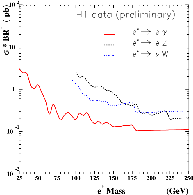
Fig. 135: Upper limits at the 95 % CL from the H1 collaboration on the product of the production cross section (in pb) and the branching ratio for excited electron production.

The latest limits attained by the H1 collaboration on the product of the production cross section times the branching ratio for excited electrons are summarized in Fig. 135. These limits are based on $37$ pb^-1 of $e^{+}p$ data accumulated from 1994-97. Similar limits for the decay $e^{*}\rightarrow e\gamma$ exist from ZEUS. The limits attained for excited neutrinos or squarks are roughly a factor of two worse than those for excited electrons due to the more difficult experimental search procedure. For final states with photons, the sensitivity is approximately $0.1$ pb. These cross section limits are independent of the particular model chosen.

Results obtained at LEP (?; ?; ?; ?) and the Tevatron (?; ?) can be compared to the HERA results for the quantity $f/\Lambda$. The LEP limits for $e^{*}$ and $\nu^{*}$ are more stringent by about a factor of two than those from HERA, but are limited to masses of $180$ GeV. The results on $q^{*}$ from the Tevatron are very strong, but require a nonzero strong coupling for the excited quarks. The HERA limits are therefore complementary.

8.4 Search for right handed currents

One of the particuliarities of the SM is that it is not left-right symmetric. It does not contain right-handed gauge bosons or neutrinos. It is important to determine whether this is only a low energy phenomena, with left-right symmetry restoration occurring at higher energies. A possible extension of the SM which is left-right symmetric is obtained via the replacement

$$SU(2)_{L}\times U(1)_{Y}\rightarrow SU(2)_{L}\times SU(2)_{R}\times U(1)^{\prime}\;\;.$$ (243)

The relationship between the electromagnetic and weak coupling constants are given in this theory by (?)

$$\frac{1}{e^{2}}=\frac{1}{g_{L}^{2}}+\frac{1}{g_{R}^{2}}+\frac{1}{g^{\prime 2}}\;\;,$$ (244)

where $g_{L},g_{R}$ are the couplings associated with the $W_{L}$ and $W_{R}$, respectively, and $e=g_{L}\sin\theta_{W}$. The coupling constant $g^{\prime}$ is associated with the $U(1)^{\prime}$ generator. In the SM, $e=g_{Y}\cos\theta_{W}$, where $g_{Y}$ is the coupling constant of $U(1)_{Y}$.

Equation 244 gives the constraint

$$g_{R}\geq g_{L}\tan\theta_{W}$$ (245)

or, $g_{R}\geq 0.55g_{L}$ . The model can therefore be invalidated if an experiment is sensitive to right-handed couplings below this value.

Fig. 136: Feynman diagram for the production of a heavy right-handed neutrino via the $t$-channel exchange of a right-handed $W$ in $e^{\pm}p$ collisions at HERA. The heavy neutrino subsequently decays into a $W^{\pm}$ and an $e^{\pm}$.

The ZEUS collaboration has searched for heavy right-handed neutrinos, $N_{e}$, produced in $e^{-}p$ and $e^{+}p$ collisions at HERA. The Feynman diagram for the process is shown in Fig. 136. Significant limits exist on right-handed neutrinos and $W$’s from other experiments (?; ?; ?; ?), but these are either very model dependent, or apply to heavy $W_{R}$’s. In general, the parameter space given by

$$M_{W_{R}} < 100\;\;{\rm GeV}\;,$$ (246)

$$M_{W_{R}} < M_{N_{e}}\;,$$ (247)

is largely unexplored by these limits. The ZEUS analysis has focused on this region (?; ?).

Fig. 137: The contours of constant 95 % CL upper limits on $g_{R}/g_{L}$ in the $M_{W_{R}},M_{N_{e}}$ plane. The areas left of the curves are excluded. For masses where ZEUS is sensitive to $g_{R}/g_{L}<0.55$, the gauge structure $SU(2)_{L}\times SU(2)_{R}\times U(1)$ is ruled out. The dotted line indicates the kinematic limit of the ZEUS search.

The experimental search generally followed the lines of the NC DIS analysis. The heavy neutrino decays into a $W_{R}$ and an electron. Evidence of the presence of a right-handed $W$ was searched for in the jet-jet invariant mass spectrum, while the presence of the right-handed neutrino was searched for in jet-jet-$e^{\pm}$ invariant mass. A well reconstructed electron was required in the final state, accompanied by at least $2$ jets. No significant signal was found, and upper limits were placed on $M_{W_{R}},M_{N_{e}}$ for different values of $g_{R}/g_{L}$. These limits are shown in Fig. 137. For $M_{W_{R}}\leq 40$ GeV and $M_{N_{e}}\approx 60$ GeV, $g_{R}<0.55g_{L}$ is ruled out. For $g_{R}=g_{L}$, $W_{R}$ masses up to $80$ GeV and $N_{e}$ masses up to $170$ GeV are ruled out.

8.5 Search for new interactions

In this section, we review the search for new interactions occurring at high mass scales $\Lambda\gg\sqrt{s}$. These interactions effectively appear as four-fermion contact interactions at HERA energy scales, in analogy with Fermi’s four-fermion contact interaction model for the weak force. A contact interaction would produce a deviation of the observed cross section, particularly at large $Q^{2}$, from the SM expectations.

If the scale of the new physics is well beyond the center-of-mass energy available, its effect can be parameterized as a four-fermion interaction. The simplest $lq\rightarrow lq$ contact interactions which conserve $SU(3)\times U(1)$ can be represented as additional terms to the Standard Model Lagrangian, $L_{SM}$, as

$$\begin{array}[]{lrlr}L=L_{SM}+&{{\displaystyle g^{2}}\over{\displaystyle\Lambda^{2}}}[&\eta_{s}\left({\bar{e}_{L}e_{R}}\right)\left({\bar{q}_{L}q_{R}}\right)+\eta^{\prime}_{s}\left({\bar{e}_{L}e_{R}}\right)\left({\bar{q}_{R}q_{L}}\right)+h.c.&{\rm scalar}\mbox{}\\ &+&\eta_{LL}\left({\bar{e}_{L}\gamma^{\mu}e_{L}}\right)\left({\bar{q}_{L}\gamma_{\mu}q_{L}}\right)+\eta_{LR}\left({\bar{e}_{L}\gamma^{\mu}e_{L}}\right)\left({\bar{q}_{R}\gamma_{\mu}q_{R}}\right)&\\ \mbox{}&+&\eta_{RL}\left({\bar{e}_{R}\gamma^{\mu}e_{R}}\right)\left({\bar{q}_{L}\gamma_{\mu}q_{L}}\right)+\eta_{RR}\left({\bar{e}_{R}\gamma^{\mu}e_{R}}\right)\left({\bar{q}_{R}\gamma_{\mu}q_{R}}\right)&{\rm vector}\\ \mbox{}&+&\eta_{T}\left({\bar{e}_{L}\sigma^{\mu\nu}e_{R}}\right)\left({\bar{q}_{L}\sigma_{\mu\nu}q_{R}}\right)+h.c.],&{\rm tensor}\end{array}$$ (248)

where $g$ is the coupling, $\Lambda$ is the effective mass scale, and $\eta$ determines the relative size and sign of the individual terms.

Strong limits exist on the scalar and tensor terms (?), so we focus here on the vector terms. The effect of the vector interactions on the cross section is the addition of an extra term to the vector and axial vector couplings for each quark flavor (see Eq. (78)),

$$\begin{array}[]{lllll}V^{L}&=&V_{SM}^{L}&+&{{Q^{2}}\over{8\pi\alpha}}{{g^{2}}\over{2\Lambda^{2}}}\left({\eta_{LL}+\eta_{LR}}\right)\;,\\ V^{R}&=&V_{SM}^{R}&+&{{Q^{2}}\over{8\pi\alpha}}{{g^{2}}\over{2\Lambda^{2}}}\left({\eta_{RL}+\eta_{RR}}\right)\;,\\ A^{L}&=&A_{SM}^{L}&+&{{Q^{2}}\over{8\pi\alpha}}{{g^{2}}\over{2\Lambda^{2}}}\left({\eta_{LL}-\eta_{LR}}\right)\;,\\ A^{R}&=&A_{SM}^{R}&+&{{Q^{2}}\over{8\pi\alpha}}{{g^{2}}\over{2\Lambda^{2}}}\left({\eta_{RL}-\eta_{RR}}\right)\;.\\ \end{array}$$ (249)

Note that the contact terms enter only as a function of $Q^{2}$, and as a consequence their relative contributions to the cross section at fixed $Q^{2}$ are approximately independent of $x$.

A commonly used convention is to set $g=\sqrt{4\pi}$ and to use $\eta$ as a sign parameter. The relative strengths of the different terms is then placed in $\Lambda$. In this convention, we write the contact interaction Lagrangian (keeping only the vector terms) as

$$L_{CI}=\sum_{i,j=L,R}\frac{4\pi}{(\Lambda_{ij}^{q})^{2}}\eta_{ij}^{q}(\bar{e}_{i}\gamma_{\mu}e_{i})(\bar{q}_{j}\gamma_{\mu}q_{j})\;,$$ (250)

where $q$ represents the quark generation. Assuming only valence quarks participate, there are 16 different scales (2 each for helicity of lepton, helicity of quark, quark flavor, and sign of $\eta$.) The limits are then placed on $\Lambda_{ij}^{q}$.

Fig. 138: The differential NC $e^{+}p$ cross section versus $Q^{2}$ compared with Standard Model expectations. The right-hand plot gives the ratio to the expectations.

The H1 (?) and ZEUS (?) collaborations have searched for contact interactions based on their 1994-97 data sets. The measurement consists effectively of comparing the measured differential cross section $d\sigma/dQ^{2}$ with SM expectations. Figure 138 shows the H1 measurement, and the ratio to the SM expectation. No significant deviation is found, and limits can be placed on the scale of possible new physics. The limits attained by ZEUS and H1 are summarized in Table 15 and compared to results from LEP (?; ?; ?) and the Tevatron (?). The limits are found to be comparable in strength.

Table 15: Selected limits on possible new contact interaction terms. The class denotes the type of interaction: $VV$, all $\eta^{q}_{ij}$ have the same sign, given by $+a$; $AA$, $\eta^{q}_{LL}$ and $\eta^{q}_{RR}$ have sign $+a$, while $\eta^{q}_{LR}$ and $\eta^{q}_{RL}$ have sign $-a$; $VA$, $\eta^{q}_{iL}$ have sign $+a$ while $\eta^{q}_{iR}$ have sign $-a$; $X3$, $\eta^{q}_{LL}$ and $\eta^{q}_{RR}$ have sign $+a$ while other terms are zero; $X4$, the complement of $X3$; and $U4$, where $\eta^{u}_{LR}$ and $\eta^{u}_{RL}$ have sign $+a$ and other terms are zero.

		Limit	Limit	Limit	Limit	Limit	Limit
		from	from	from	from	from	from
		H1	ZEUS	CDF	OPAL	ALEPH	L3
Class	$a$	$\Lambda$(TeV)	$\Lambda$(TeV)	$\Lambda$(TeV)	$\Lambda$(TeV)	$\Lambda$(TeV)	$\Lambda$(TeV)
$VV$	$+1$	4.5	4.9	3.5	3.3	4.0	3.2
$VV$	$-1$	2.5	4.6	5.2	4.3	5.2	3.9
$AA$	$+1$	2.0	2.0	3.8	4.9	5.6	4.3
$AA$	$-1$	3.8	4.0	4.8	3.1	3.7	2.9
$VA$	$+1$	2.6	2.8	$-$	$-$	$-$	$-$
$VA$	$-1$	2.8	2.8	$-$	$-$	$-$	$-$
$X3$	$+1$		2.8	$-$	3.5	4.1	3.2
$X3$	$-1$		1.5	$-$	2.9	3.6	2.8
$X4$	$+1$		4.5	$-$	2.5	3.0	2.4
$X4$	$-1$		4.1	$-$	4.1	4.9	3.7
$U4$	$+1$		4.6	$-$	2.0	2.1	1.8
$U4$	$-1$		4.4	$-$	2.3	2.6	2.2

Other limits come from several sources. Atomic parity violation experiments place stringent limits on possible contact interactions (?). These can however be avoided if $\eta_{LL}+\eta_{LR}-\eta_{RL}-\eta_{RR}=0$. A comprehensive review can be found in ?.

8.6 Observation of high $p_{T}$ lepton events

Fig. 139: Display of the $\mu^{+}$ event (MUON-1). Shown are a side view (left) and a transverse view of the event. The “Legoplot” shows the observed calorimetric energy depositions in the $\eta-\phi$ plane.

The H1 collaboration has observed an excess of events consisting of an isolated electron or muon of high transverse momentum and a high $p_{T}$ jet. The events also have a large imbalance in transverse momentum. One such event had previously been reported based on the analysis of the 1994 data (?; ?). This event is shown in Fig. 139. Analysis of all the data from 1994-1997, giving an integrated luminosity of $36.5$ pb^-1, has resulted in the observation of an additional 5 events (?). The ZEUS collaboration has so far no evidence for this type of event (?).

8.6.1 Analysis procedure

The event selection follows the line of the standard H1 charged current event selection (?). The basic requirement is a large imbalance in the transverse energy as measured in the calorimeter, $p_{T}^{calo}>25$ GeV. Additionally, a tracking vertex is required, and topological and timing filters are applied to remove backgrounds from the sample. This selection produces a clean sample of charged current events, which contain typically one high $p_{T}$ jet. Events are then searched for with tracks with transverse momentum, $p_{T}>10$ GeV. Six events are observed where the track is far from the jet and any other track in the event. These tracks all correspond to either an electron or a muon. The event shown in Fig. 139 is typical of these events. The events are very clean and well reconstructed.

8.6.2 Results

The event properties are listed in Table 16. Four of the events contain a single high $p_{T}$ muon (MUON1, MUON2, MUON4, MUON5), one contains a single high $p_{T}$ electron, and one contains a high $p_{T}$ muon (MUON3) and a low $p_{T}$ electron. The five muon events have hadronic transverse momentum ranging from $27-67$ GeV. The electron event has a hadronic $p_{T}$ of only $8$ GeV.

Table 16: Reconstructed event kinematics for H1 events containing a high $p_{T}$ lepton and large missing transverse momentum . Energies, momenta and masses are given in GeV and angles in degrees. For the charge of the high-$P_{T}$ lepton the significance of the determination is given. In case of event MUON-5 $2\sigma$ limits are quoted for the muon momentum and derived quantities.

	ELECTRON	MUON-1	MUON-2	MUON-3 *)	MUON-4	MUON-5
The isolated high-$P_{T}$ lepton
Charge	Neg.( $5\sigma$)	Pos.( $4\sigma$)	Pos.( $4\sigma$)	Neg.( $4\sigma$)	Neg.( $2\sigma$)	unmeasured
$P_{T}^{l}$	$37.6^{+1.3}_{-1.3}$	$23.4^{+7.5}_{-5.5}$	$28.0^{+8.7}_{-5.4}$	$38.6^{+12.0}_{-7.4}$	$81.5^{+75.2}_{-26.4}$	$>44$
$\theta^{l}$	$27.3\pm 0.2$	$46.2\pm 0.1$	$28.9\pm 0.1$	$35.5\pm 0.1$	$28.5\pm 0.1$	$31.0\pm 0.1$
The hadronic system
$P_{T}^{X}$	$8.0\pm 0.8$	$42.2\pm 3.8$	$67.4\pm 5.4$	$27.4\pm 2.7$	$59.3\pm 5.9$	$30.0\pm 3.0$
$P_{\|}^{X}$	$-7.2\pm 0.8$	$-42.1\pm 3.8$	$-61.9\pm 4.9$	$-12.5\pm 2.1$	$-57.0\pm 5.5$	$-28.6\pm 3.1$
$P_{\bot}^{X}$	$-3.4\pm 0.9$	$-2.7\pm 1.8$	$26.8\pm 2.7$	$-24.3\pm 2.5$	$-16.3\pm 3.2$	$-9.1\pm 2.3$
$P_{z}^{X}$	$79.9\pm 4.4$	$153.1\pm 9.1$	$247.0\pm 18.9$	$183.7\pm 13.6$	$118.9\pm 12.1$	$145.4\pm 8.2$
$E^{X}$	$81.1\pm 4.5$	$162.0\pm 10.0$	$256.9\pm 19.5$	$186.8\pm 14.0$	$141.7\pm 13.7$	$154.8\pm 9.1$
Global properties
$P_{T}^{miss}$	$30.6\pm 1.5$	$18.9^{+6.6}_{-8.3}$	$43.2^{+6.1}_{-7.7}$	$42.1^{+10.1}_{-5.9}$	$29.4^{+71.8}_{-13.9}$	$>18$
$\delta$	$10.4\pm 0.7$	$18.9^{+3.9}_{-3.2}$	$17.1^{+2.5}_{-1.7}$	$26.9^{+4.2}_{-2.9}$	$43.5^{+19.3}_{-7.2}$	$>22$
$M_{T}^{l\nu}$	$67.7\pm 2.7$	$3.0^{+1.5}_{-0.9}$	$22.8^{+6.7}_{-4.2}$	$75.8^{+23.0}_{-14.0}$	$94^{+157}_{-54}$	$>54$
∗) Positron in MUON-3 :
$P_{T}^{e}=6.7\pm 0.4$ , $P_{\|}^{e}=6.1\pm 0.4$, $P_{\bot}^{e}=-2.8\pm 0.2$ , $P_{z}^{e}=-3.7\pm 0.2$

The main process expected to yield high $p_{T}$ leptons in events with missing transverse energy is photoproduction of $W$ bosons, with subsequent leptonic decays. The $W$ is predominantly produced radiatively from the scattered quark. This process is calculable in LO and has been quantitatively evaluated (?), yielding a total cross section of about $70$ fb per lepton species and charge. The hadronic $p_{T}$ expected from $W$ production is generally small, while the transverse lepton-$\nu$ mass has a Jacobian peak near the $W$ mass.

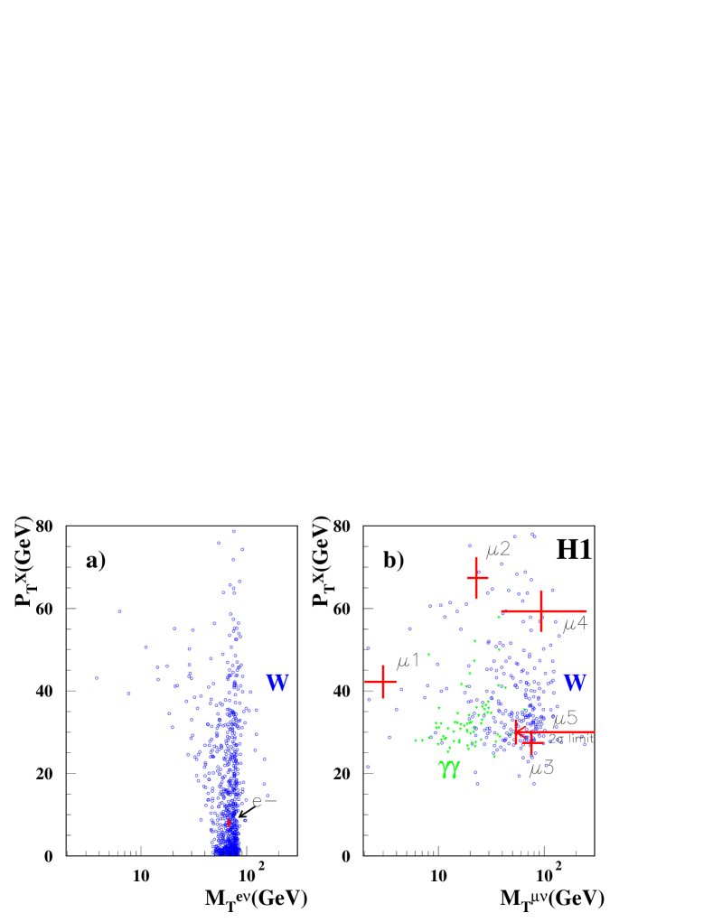
Fig. 140: Distribution of the six events in $p_{T}^{X}$ and $M_{T}^{l\nu}$:a) electron channel; b) muon channel. The crosses correspond to the 1-sigma uncertainty on the measured parameters of each event. The points show the standard model expectation for $W$ production for an accumulated luminosity a factor $500$ higher than in the data.

The events are compared to expectations from a $W$ Monte Carlo sample corresponding to a luminosity 500 times that of the data in Fig. 140. The muon events MUON1, MUON2 and MUON4 are in regions with small expectations. After applying the analysis cuts, H1 expects $2.4\pm 0.5$($0.8\pm 0.2$) events in the $e^{\pm}$($\mu^{\pm}$) channels respectively, of which $1.7\pm 0.5$($0.5\pm 0.1$) are expected from the LO calculations for $W$ production. Two of the observed events are consistent with the $W$ interpretation (ELECTRON, MUON3). A second muon event, MUON5, is compatible, within the large measurement errors, with $W$ production.

The ZEUS experiment has reported on a search for these events using a very similar analysis procedure (?), but has found no electron or muon events with large missing $p_{T}$ and large hadronic $p_{T}$.

8.6.3 Discussion

The events observed by the H1 collaboration are clean and well reconstructed. The ZEUS detector has a very similar acceptance and reconstruction capability for these types of events, and should therefore also have seen a signal if there was a large cross section for new physics. The non-observation of events by ZEUS can be accomodated with reasonable probability by assuming that the true expectation is roughly $1/2$ what H1 measures. It remains to be seen whether such a cross section can be reproduced by higher order calculations for $W$ production, or whether new physics mechanisms beyond the Standard Model are necessary.

8.7 Observation of events at large $x$ and large $Q^{2}$

The H1 and ZEUS Collaborations reported an excess of events at large $x$ (or $M_{eq}$) and large $Q^{2}$ in early 1997 (?; ?). In the case of H1, 12 neutral current events were observed for $Q^{2}>15000$ GeV² where $4.71\pm 0.76$ were expected. In the same $Q^{2}$ range, H1 observed $4$ charged current events where $1.77\pm 0.87$ were expected. For the NC case, the excess is most prominent around $M_{eq}=200$ GeV, where 7 events were observed with $y>0.4$ in a mass window of width $25$ GeV, where only $0.95\pm 0.18$ events were expected. ZEUS observed two events for $Q^{2}>35000$ GeV² where $0.145\pm 0.013$ were expected, while for $x>0.55$ and $y>0.25$, four events were observed where $0.91\pm 0.08$ events were expected. The analyses, while each not statistically compelling, generated interest because they occured in previously unexplored kinematic regions. At large $Q^{2}$, non-DIS backgrounds are estimated to be below 1 % and the uncertainty of the SM predictions is below 10 %. The samples of events are background free, and can be compared to precise predictions of the Standard Model. This is an ideal experimental situation.

8.7.1 Interpretations of the HERA events

The HERA observations have generated intense theoretical analysis of possible underlying causes. We briefly review a selection of these analyses.

• Several authors have attempted to modify the parton distributions at large-$x$ within the experimentally allowed range to see how big a variation could be produced at large $x\;{\rm and}\;Q^{2}$. As mentioned above, ZEUS and H1 concluded that the SM predictions were quite precise. This was based on existing fixed target measurements of structure functions, conventional forms for the parton density parameterizations, and NLO DGLAP evolution of the parton densities. Some of these assumptions can be questioned, such as the functional form of the quark densities at large $x$. For example, ? have added an extra component to the valence $u$-quark density of the form $0.02(1-x)^{0.1}$, which would be compatible with existing data. While they find a $30$ % effect for $Q^{2}=40000$ GeV² at $x=0.7$, the effect in the $x$ range relevant for the HERA effect ($x=0.4-0.6$) is considerably smaller. ? point out that intrinsic charm in the proton is expected to give a contribution at large $x$, with a peak in the vicinity of $M=200$ GeV. However, existing data constrains the cross section enhancement due to intrinsic charm to 15 %.

  The use of the NLO DGLAP evolution to predict the cross sections at large $Q^{2}$ have also been called into question. ? argues that instanton induced quark-gluon interactions, a non-perturbative effect, will be proportionally more important at large $Q^{2}$. The cross sections estimated with the NLO DGLAP equations alone would therefore be an underestimate, possibly by as much as 50 %.

• The possibility of a leptoquark as the source of the events has been considered by many authors. For example, see (?; ?; ?). The clustering of H1 events near $200$ GeV make the LQ interpretation an intriguing possibility. The combined ZEUS+H1 cross section for the events near $200$ GeV is roughly

  $$\sigma\approx\frac{10\;\rm{event}}{35\;\rm{pb}^{-1}}\approx 0.3\rm{pb}\;\;.$$ (251)

  This can be used to estimate the size of the LQ coupling strength to the lepton-quark pair, as discussed in section 8.1. The cross section is very strongly dependent on the quark or antiquark density involved. We assume the production is off valence quarks given the large suppression of sea quarks at the large values of $x$ involved. Taking an up quark density of about $0.15$ and a down quark density $4$ times smaller (see Fig. 50) yields a value of $\lambda\approx 0.025/\sqrt{B}$ for an $e^{+}u$ scalar LQ, where $B$ is the branching fraction into $e^{+}q$. The corresponding coupling for an $e^{+}d$ LQ would be twice as large.

  Note that LQ production can proceed via $q\bar{q}$ or $gg$ fusion at the Tevatron independently of the coupling $\lambda$. This allows D0 (?) and CDF (?) to set limits on a scalar LQ mass of $225$ GeV and $213$ GeV, respectively. The bounds assume a 100 % branching ratio to $eq$, and are considerably reduced for smaller branching ratios. The cross section for vector LQ production in $p\bar{p}$ collisions is model dependent, but is expected to be much larger than that for scalar production (?; ?). It is therefore expected that vector LQ are unlikely.

• ${\textstyle\not{R}_{P}}$ squarks have been proposed as an alternative mechanism for producing a resonance near $200$ GeV (see, for example, (?; ?)). As described in section 8.2.2, ${\textstyle\not{R}_{P}}$ squarks can be produced by the fusion of a positron with a $d$-type quark to a $u$-type antiquark. Given the large $x$ values involved, we consider only production from $d$-quarks. ${\textstyle\not{R}_{P}}$-squark production can be differentiated from LQ production since different decay modes are possible. In particular, in addition to the Yukawa decay ${\tilde{u}}\rightarrow e^{+}d$, the squark can also decay via gauge couplings ${\tilde{u}}\rightarrow c\chi^{0}_{i(i=1,4)},s\chi^{+}_{j(j=1,2)}$.

  Strong limits exist from neutrinoless double beta decay (?; ?) which make the ${\tilde{u}}_{L}$ scenario very unlikely. The production of $\widetilde{t}_{L}$ is limited by atomic parity violation (?). A detailed analysis (?) leads to the $\widetilde{c}_{L}$ squark as the most likely candidate. It is found that a branching ratio to $e^{+}d$ near one is favored, so that any sizeable signal in the CC mode would make this scenario unlikely. No signal would be expected in $e^{-}p$ collisions. Also, other reactions such as $K^{+}\rightarrow\pi^{+}\nu\bar{\nu}$ should become visible at experiments with increased sensitivity. This scenario should therefore be within experimental reach very soon.

• Finally, contact interactions (see section 8.5) representing the effect of some new interaction at a mass scale $\Lambda\gg\sqrt{s}$ have been analyzed as a possible source of excess events at large $Q^{2}$ by many authors. In particular, ? have made a global study of all data relevant to $eeqq$ contact interactions, including deep inelastic scattering data, atomic parity violation experiments, polarized $e^{-}$ scattering on nuclear targets, Drell-Yan production at the Tevatron, the total hadronic cross section at LEP and neutrino-nucleon scattering data. They conclude that contact interaction terms of the type $\eta^{eu}_{LR}$ and $\eta^{eu}_{RL}$ give the best fit to the HERA data while the $eeuu$ contact interactions are severely limited by the Drell-Yan data. Using a global fit to all the data, the authors find that all contact interaction interpretations are strongly constrained.

Many more scenarios have been proposed beyond those described above. Clearly, more experimental data is needed to resolve which, if any, of these approaches is correct, or if the effect is due to a statistical fluctuation.

8.7.2 Data sets

Both collaborations have updated their analyses using the 1997 data. We review the status of the analyses as presented at the LP97 Symposium (?). These results from the H1 and ZEUS collaborations include data up to the end of June, 1997. The corresponding integrated luminosities are $23.7$ pb^-1 for H1 and $33.5$ pb^-1 for ZEUS.

8.7.3 Charged current analysis

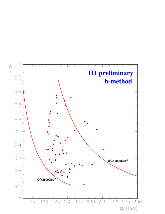
Fig. 141: The distribution in $M$ and $y$ of the H1 charged current event sample. The curves show contours of constant $Q^{2}$.

Fig. 142: The distribution in $x$ and $y$ of the ZEUS charged current event sample. The curves show contours of constant $Q^{2}$.

The charged current (CC) analysis relies primarily on the selection of events with large missing transverse momentum. H1 requires events to have at least $50$ GeV of missing $p_{T}$, while ZEUS requires $p_{T}>15$ GeV and $Q^{2}>1000$ GeV². With these cuts, the backgrounds are found to be negligible. The distribution of events observed by H1 is plotted in the plane of $y$ versus $M$ in Fig. 141, while the ZEUS event distribution in shown in the plane of $y$ versus $x$ in Fig. 142. A typical large $Q^{2}$ CC event as observed in the H1 detector is shown in Fig. 143. The event consists of a single high energy jet and energy deposits from the proton remnant.

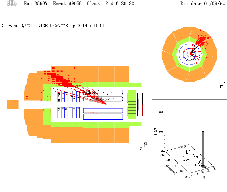
Fig. 143: A high $Q^{2}$ charged current event, as observed in the H1 detector. The left part shows the H1 inner tracking system and the calorimeter. The filled rectangles in the calorimeter denote energy deposits which are above the noise thresholds. The upper right display shows a projection onto a plane perpendicular to the beam axis, where only barrel calorimeter energy deposits are shown. The lower right part of the figure shows the calorimeter transverse energy deposits in the $\eta-\phi$ plane. The scattered quark jet dominates the event. The event parameters are given in the display.

The numbers of observed and expected events are compared in Table 17. The data lie above expectations for $Q^{2}>10000$ GeV². For $Q^{2}>15000$ GeV², a total of $11$ events are observed where $4.9\pm 1.7$ are expected. For $Q^{2}>30000$ GeV², ZEUS observes one event where $0.03\pm 0.04$ are expected. Note that the number of expected and observed events in ZEUS and H1 do not scale with the luminosity at large $Q^{2}$. This is due to differences in the analysis. The ZEUS data are partially unfolded for detector smearing, using a CC MC, and this tends to reduce both the expectations and the number of observed events at large $Q^{2}$.

Table 17: Preliminary 1994-1997 results as of the Lepton-Photon 97 Symposium on the numbers of charged current events observed ($N_{obs}$) by H1 and ZEUS above various $Q^{2}$ cuts compared to SM expectations ($N_{exp}$). The columns labeled $\delta N_{exp}$ give the uncertainty on the SM expectations. For ZEUS separate uncertainties on the SM expectation are quoted for the uncertainty on the energy scale and the uncertainty in the parton density functions.

$Q^{2}$ cut	H1			ZEUS
(GeV2)	$N_{obs}$	$N_{exp}$	$\pm\delta N_{exp}$	$N_{obs}$	$N_{exp}$	$\pm\delta N_{exp}$	$\pm\delta N_{exp}$
						(E)	(PDF)
$Q^{2}>1000$				455	419	$\pm 13$	$\pm 33$
$Q^{2}>2500$	61	56.3	$\pm$ 9.40	192	178	$\pm 13$	$\pm 17$
$Q^{2}>5000$	42	34.7	$\pm$ 6.90	63	58.5	$\pm 9.0$	$\pm 7.3$
$Q^{2}>10000$	14	8.33	$\pm$ 3.10	15	9.4	$\pm 2.5$	$\pm 1.6$
$Q^{2}>15000$	6	2.92	$\pm$ 1.44	5	2.0	${}^{+0.81}_{-0.54}$	$\pm 0.4$
$Q^{2}>20000$	3	1.21	$\pm$ 0.64	1	0.46	${}^{+0.28}_{-0.16}$	$\pm 0.10$
$Q^{2}>30000$				1	0.034	${}^{+0.037}_{-0.016}$	$\pm 0.008$

8.7.4 Neutral current analysis

The neutral current (NC) event selection relies primarily on the observation of an isolated high energy electron and conservation of longitudinal ($E-P_{Z}$) and transverse momentum. H1 considers events for which $Q^{2}>2500$ GeV², while ZEUS starts at $Q^{2}>5000$ GeV². Both collaborations conclude that the data sets are background free.

ZEUS and H1 have used different reconstruction methods. H1 has chosen the electron method as the primary method, with the double angle method as check, while ZEUS has chosen the double angle method as primary method, with the electron method as check. The two methods each give good resolutions at large $y$, with rapidly degrading resolution as $y\rightarrow 0$. The methods behave differently in the presence of initial state QED radiation from the electron. The double angle method is more sensitive to ISR, and the $x$ is always overestimated in the presence of radiation from the electron. These effects are however expected to be small. ZEUS achieves a resolution of $5-10$ % in $x$ and 5 % in $Q^{2}$, while H1 finds a resolution of about $2/y$ % for $x$.

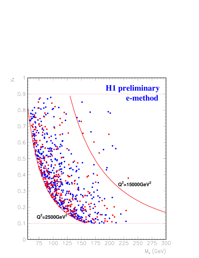
Fig. 144: The distribution in $M$ and $y$ of the H1 neutral current sample. The curves show contours of constant $Q^{2}$.

Fig. 145: The distribution in $x$ and $y$ of the ZEUS neutral current sample. The curves show contours of constant $Q^{2}$.

The distribution of events measured by the H1 collaboration are shown in the $M,y$ plane in Fig. 144, while the ZEUS results are shown in the $x,y$ plane in Fig. 145. A typical large $Q^{2}$ event as measured in the ZEUS detector is shown in Fig. 146.

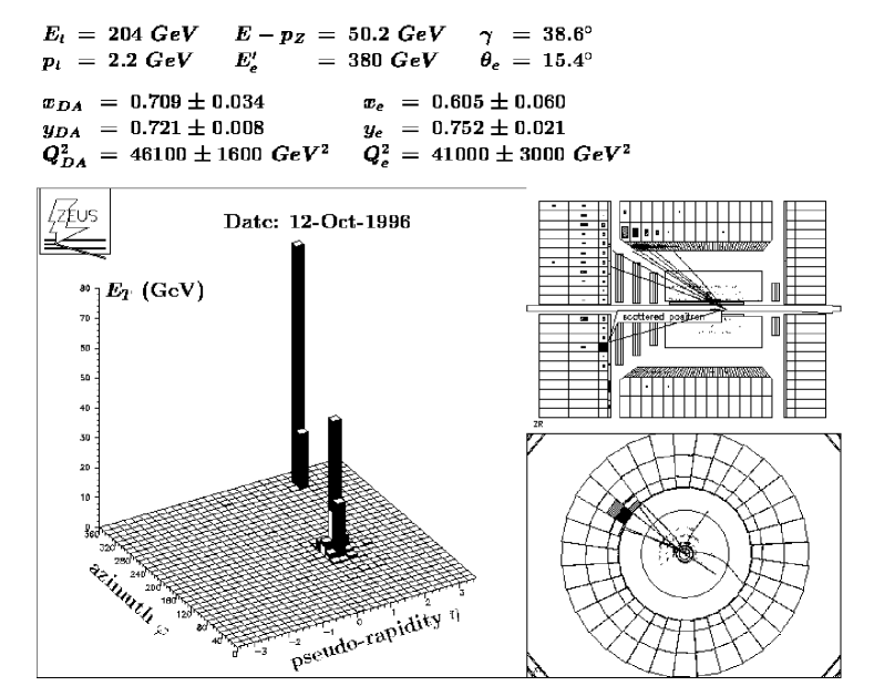
Fig. 146: The largest $Q^{2}$ neutral current event recorded at HERA to date, as observed in the ZEUS detector. The top right part shows the ZEUS inner tracking system and the calorimeter. The filled rectangles in the calorimeter denote energy deposits which are above the noise thresholds. The bottom right display shows a projection onto a plane perpendicular to the beam axis, where only barrel calorimeter energy deposits are shown. The left part of the figure shows the calorimeter transverse energy deposits in the $\eta-\phi$ plane, and demonstrates that the electron and the scattered quark jet dominate the event. The event parameters are given above the event display.

Table 18: Number of events observed ($N_{obs}$) by H1 compared to SM NC DIS expectations ($N_{exp}$) in several kinematic regions. The first term in each sum gives the 1994-1996 value and the second term gives the 1997 value as of the Lepton-Photon 97 Symposium.

region	$N_{obs}$	$N_{exp}$
$Q^{2}>2500$  GeV2	443+281=724	427+287=714$\pm$69
$Q^{2}>15000$  GeV2	12+6=18	4.7+3.3=8.0$\pm$1.2
$187.5<M<212.5$  GeV	7+1=8	0.95+0.58=1.53$\pm$0.29
and $y>0.4$

The numbers of events in different kinematic regions as measured by H1 are summarized in Table 18. The numbers of observed and expected events are given separately for the 1994-96 running period, and for the partial 1997 data set. As is seen, the excess in the mass window centered on $200$ GeV did not increase in significance with the addition of the 1997 data. However, the number of large $Q^{2}$ events continued to accumulate at a rate higher than expected from the SM. The $Q^{2}$ and $M$ distributions as measured by H1 are given in Fig. 147 and Fig. 148.

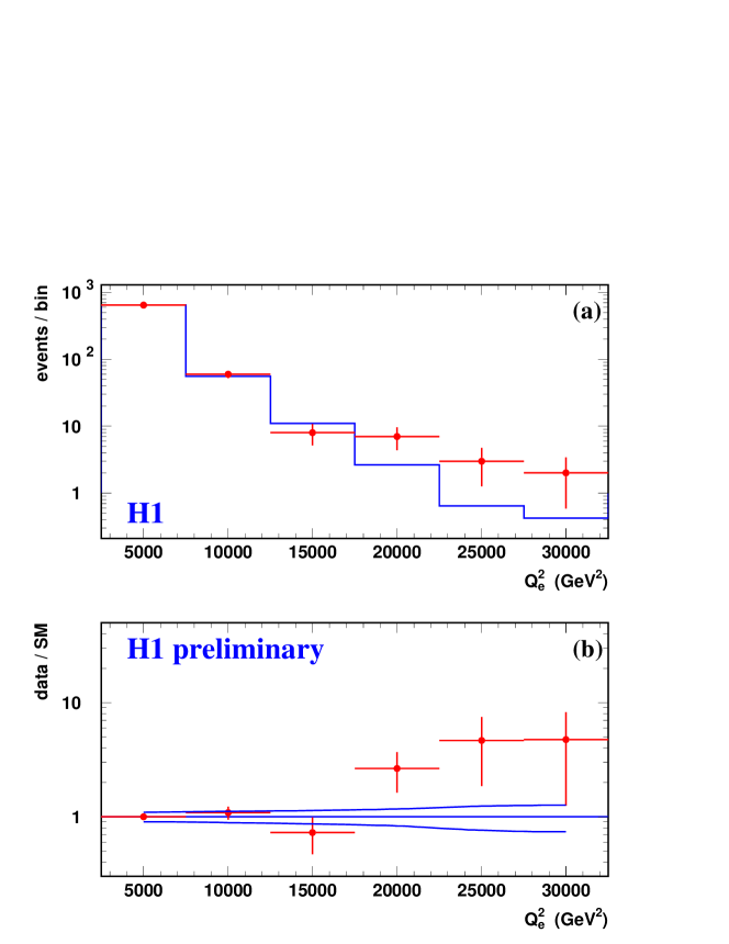
Fig. 147: The upper plot shows the $Q^{2}$ spectrum for the H1 neutral current sample. The points with error bars indicate the data and the histogram shows the NC DIS expectations. The lower plot shows the $Q^{2}$ spectrum divided by the SM expectations. The smooth curves indicate the uncertainty in the expectations.

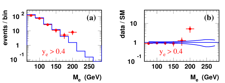
Fig. 148: The upper plot shows the $M$ spectrum for $y>0.4$ for the H1 neutral current sample. The points with error bars indicate the data and the histogram shows the NC DIS expectations. In the lower plot the points give the ratio of the number of events observed to the NC DIS expectations and the smooth curves give the uncertainty in the expectations.

The combined H1 data sample show a clear excess of observed events over expectations starting at $Q^{2}>15000$ GeV². For $Q^{2}>15000$ GeV², 18 events are observed where $8.0\pm 1.2$ are expected, corresponding to a probability of $0.34~{}\%$. The excess of events near $M=200$ GeV remains prominent. For 187.5 GeV $<M<$ 212.5 GeV, 8 events are observed while $1.53\pm 0.29$ are expected, corresponding to a probability of $3.3\times 10^{-4}$. The probability to see an excess this significant in some $M$ window is $\sim 1\%$.

Fig. 149: The upper plot shows the $Q^{2}$ spectrum for the ZEUS neutral current sample. The points with error bars indicate the data and the histogram shows the NC DIS expectations. In the lower plot the dotted curve and the solid curve show respectively the number of events expected and the number observed with $Q^{2}>Q^{2*}$ vs. $Q^{2*}$.

Fig. 150: The upper plot shows the $x$ spectrum for $y>0.25$ of the ZEUS neutral current sample. The points with error bars indicate the data and the histogram shows the NC DIS expectations. In the lower plot the dotted curve and the solid curve show respectively the number of events expected and the number observed with $x>x^{*}$ vs. $x^{*}$.

Table 19: Number of events observed ($N_{obs}$) by ZEUS compared to SM NC DIS expectations ($N_{exp}$) in several kinematic regions. The first term in each sum gives the 1994-1996 value and the second term gives the 1997 value as of the Lepton-Photon 97 Symposium.

region	$N_{obs}$	$N_{exp}$
$Q^{2}>5000$  GeV2	191+135=326	197+130=328$\pm$15
$Q^{2}>15000$  GeV2	13+5=18	8.66+5.77=14.4$\pm$1.1
$Q^{2}>35000$  GeV2	2+0=2	0.145+0.097=0.242$\pm$0.017
$x>0.55,y>0.25$	4+1=5	0.91+0.61=1.51$\pm$0.13

The numbers of events measured by ZEUS in the signal region defined in the publication based on the 1994-96 publication are summarized in Table 19. As with H1, the numbers of observed and expected events are given separately for the 1994-96 running period, and for the partial 1997 data set. The numbers of events observed by ZEUS in these kinematic regions are close to the SM expectations. The $Q^{2}$ and $x$ distributions as measured by ZEUS are given in Fig. 149 and Fig. 150. The ZEUS measured $Q^{2}$ spectrum is in reasonable agreement with the SM up to about $Q^{2}=30000$ GeV². For $Q^{2}>35000$ GeV², 2 events are observed and $0.24\pm 0.02$ are expected, corresponding to a probability of $2.5\%$. The $x$ spectrum shows an enhancement near $x=0.55$. For $x>0.55$ and $y>0.25$, 5 events are observed while $1.51\pm 0.13$ are expected, corresponding to a probability of $1.9\%$.

Comparison of H1 and ZEUS $x(M)$ Spectra

For $y>0.4$, H1 has observed $8$ events where $1.53\pm 0.29$ were expected in the mass window $187.5<M<212.5$ GeV. This corresponds to the $x$ range $0.389<x<0.500$. In this range, ZEUS observes $3$ events where $2.92\pm 0.24$ events are expected. In the region $x>0.55,y>0.25$, ZEUS observes $5$ events where $1.51\pm 0.13$ are expected. In this region, corresponding to $M>223$ GeV, H1 observes one event, where $0.75\pm 0.30$ are expected. I.e., combining the H1 and ZEUS results does not increase the significance of either effect. A study of the possible systematic shifts in the reconstruction has led to the conclusion that the ZEUS and H1 events are unlikely to come from a single narrow resonance in $x(M)$ (?).

8.7.5 Conclusion

The full 1994-97 data has recently become available. No further evidence was seen for either an excess near $200$ GeV (?; ?) nor for an enhanced cross section at high $Q^{2}$ (?; ?; ?). Both H1 and ZEUS have therefore proceeded to set limits on leptoquark and R-parity violating squark production, as reported in previous sections. The NC and CC cross sections have been discussed in section 4.5.

The 1997 data sets did not increase the significance of the results based on the 1994-1996 data. However, there is a general tendency for the HERA data to lie above Standard Model expectations at large $Q^{2}$. This is true for the charged current as well as the neutral current events. The probability to observe the combined counting rates are a few % in each case. It is clear that the confirmation or ruling out of possible new physics will need substantially increased luminosities. The future HERA running program, outlined below, should provide the data necessary for this.

9 Outlook for HERA

9.1 The HERA luminosity upgrade

The luminosity of HERA has reached instantaneous values of $L\simeq 1.4\cdot 10^{31}$ cm^-2s^-1, which is close to the design value. The progress over the years has been steady, as can be seen in Fig. 13. This luminosity has allowed the HERA experiments to perform many important measurements, including the observation of the rise of the structure function $F_{2}$ with decreasing $x$, the observation and study of events with a large rapidity gap in the hadronic final state, the observation of resolved photon interactions, and many others. It must however be noted that most of the physics done so far is ‘small $Q^{2}$ physics’ compared with the electroweak scale of $Q^{2}=m_{W}^{2}$. The physics on the electroweak scale has so far been barely touched. This is the region HERA was built to explore. The unique features of HERA, such as electron polarization and the capability to compare electron and positron interactions are relevant only in the electro-weak regime. A luminosity upgrade bringing integrated luminosities to the level of $1$ fb^-1 by 2005 would open the possibility for many more exciting measurements. The excess of events observed by both the ZEUS and H1 experiments at large $x$ and $Q^{2}$ has put even more priority on this luminosity upgrade.

Given this strong motivation, the HERA machine group, in conjunction with members of the ZEUS and H1 experiment, have studied different alternatives to achieve the desired luminosity upgrade. The solution chosen is to install superconducting combined function (focusing and bending) magnets in the interaction regions and to rebuild focusing magnets near the interaction regions, thereby significantly reducing the beam cross sections. Instantaneous luminosities of $7.4\cdot 10^{31}$ cm^-2 s^-1 are expected in this configuration, leading to delivered integrated luminosities of about $150$ pb^-1 per year per experiment.

In addition to the luminosity upgrade machine elements, spin rotators will also be installed as planned. This will allow data taking with different electron (or positron) longitudinal polarization.

9.2 Future physics at HERA

9.2.1 Excess at large $\boldmath x,Q^{2}$

The ZEUS and H1 experiments both reported an excess of large-$x,Q^{2}$ events as described in section 8.7. The combined ZEUS and H1 cross section for $Q^{2}>15000$ GeV² reported at the LP97 conference (?) is $0.71^{+0.14}_{-0.12}$ pb, compared to the Standard Model expectation of $0.49$ pb. For $Q^{2}>30000$ GeV², the combined cross section is $0.098^{+0.059}_{-0.042}$ pb, compared to the Standard Model expectation of $0.023$ pb.

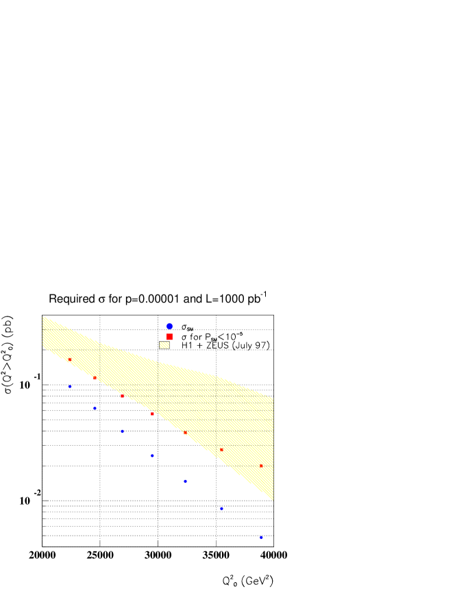
Fig. 151: The cross section necessary to produce a deviation from the Standard Model at the $10^{-5}$ level is plotted, and compared to the Standard Model cross section. Note that the integrated cross section above $Q^{2}_{0}$ is shown. These cross sections are compared to the current (LP97 status) cross sections measured by ZEUS and H1.

If the excess at large $Q^{2}$ is confirmed, it signals new physics beyond the Standard Model. It will be very difficult to confirm the effect with the present HERA luminosity. However, with an accumulated $1$ fb^-1 of luminosity, a significant deviation from Standard Model expectations will be measured if the current cross section is close to the true value. This is shown in Fig. 151, where the cross section required for a significant deviation from the Standard Model (probability for a fluctuation less than $10^{-5}$, including an estimate of the systematic errors on the cross section measurements) is compared to both the Standard Model expectations and the cross section measurements from ZEUS and H1. As can be seen from this figure, the present cross section levels would result in a very significant effect.

If the central value of the cross section currently measured by ZEUS and H1 were accurate, then a sample of order $500$ events will be available per experiment for $Q^{2}>15000$ GeV², allowing the study of a new field of physics.

The luminosity increase can be compared to an increase of the beam energies. For example, a luminosity increase by a factor 4 is roughly equivalent to an increase of the proton beam energy from 820 GeV to 1160 GeV. This type of energy increase of the machine is prohibitively expensive. The planned increase in luminosity is therefore the best way to access new physics at HERA. The proton beam energy is expected to increase to a value above 900 GeV, which can be done with minimum impact on the current machine. In fact, it is hoped that this higher energy running will already take place in 1998 . This improvement will add to the physics capability of the machine. As an example the production cross section of 240 GeV leptoquarks is increased by a factor of 2 as the proton beam energy is increased from 820 GeV to 920 GeV. Increasing the electron (positron) beam energy has also been discussed but is determined to be too expensive.

9.2.2 Physics reach with the luminosity upgrade

In the following, we review some of the conclusions of the workshop ‘Future Physics at HERA’ (ed. Ingelman, De Roeck and Klanner). The workshop consisted of several working groups: Structure Functions, Electroweak Physics, Beyond the Standard Model, Heavy Quark Production and Decay, Jets and High-$E_{T}$ Phenomena, Diffractive Hard Scattering, Polarized Protons and Electrons, Light and Heavy Nuclei, and a group studying the HERA upgrade. The results are summarized in a 1200 page report. It is obviously not possible to do justice to the full range of physics topics covered in this document. A few examples are chosen to give an indication of the physics reach achievable with the upgraded luminosity.

Fig. 152: Simulated structure function data sets. The luminosity of 1 fb^-1 will lead to precise data even at very large $Q^{2}$. For $Q^{2}\geq 10000$ GeV² about 2000 events will be available. The curve represents a NLO QCD fit. The large $x$, small $Q^{2}$ region can not be accessed with HERA but is almost completely covered by the fixed target experiment data, not shown here.

Fig. 153: Determination of gluon distribution using future $F_{2}$ data from electron-proton scattering. Note that for simplicity the gluon is shown also outside the allowed region of $x\leq Q^{2}(\,\mathrm{GeV^{2}})/10^{5}$.

The exploration of the proton structure and QCD can be continued with much larger data sets and better tools. The structure function $F_{2}$ will be measured to higher precision, over an extended kinematic region, allowing an extraction of the gluon density with an experimental precision of $1$ %. An example of what can be achieved in the measurement of $F_{2}$ is shown in Fig. 152. The corresponding gluon density is shown in Fig. 153. These very precise measurements will provide stringent tests of the QCD evolution equations. They will also provide important experimental input for cross section calculations for future accelerators utilizing hadrons. Experimental precision levels of $0.001$ on $\alpha_{s}(m_{Z}^{2})$ will be possible by combining HERA structure function data with fixed target data.

The ability to run HERA with both electrons and positrons will allow an extraction of $F_{3}$, and therefore will give a measurement of the valence quark distributions. If HERA is also run with deuterons, then the experiments can make direct measurements of the (up - down) quark distribution, which has so far not been measured. Other important QCD tests will consist of precision measurements of charm and beauty production. The study of diffraction will be significantly enhanced with increased statistics. The luminosity upgrade will allow the study of diffractive processes, such as exclusive vector meson production, at large $Q^{2}$ where perturbative QCD calculations are applicable. The study of jets will be performed at high $E_{T}$, resulting in measurements of $\alpha_{s}$ at different scales. Sensitive searches for novel phenomena predicted in QCD such as instanton production will also be performed. It is clear that a high luminosity HERA will provide precise measurements of many cross sections which should be calculable in QCD, thereby providing stringent tests of our theoretical understanding of the strongest force in nature.

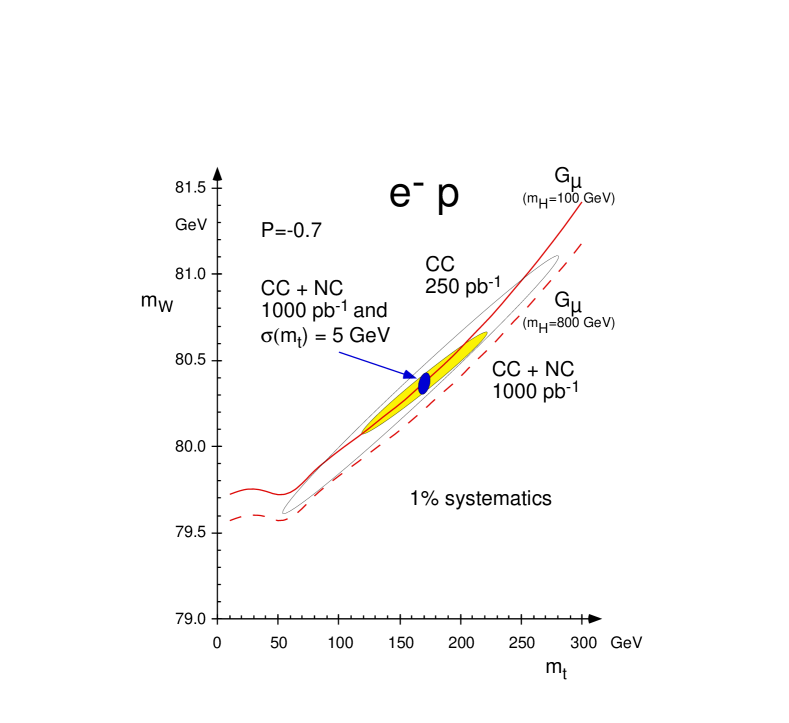
Fig. 154: The 1$\sigma$-confidence contours in the $(m_{W},m_{t})$ plane from polarized electron scattering (P=-0.7), utilizing charged current scattering at HERA only with an integrated luminosity of $250$ pb^-1 (large ellipse), neutral and charged current scattering with $1000$ pb^-1 (shaded ellipse), and the combination of the latter with a direct top mass measurement with a precision $\sigma_{m_{t}}=5$ GeV (full ellipse). The $m_{W}$-$m_{t}$ relation from the $G_{\mu}$ constraint is also shown for two values of $m_{H}$.

Sensitive tests of the electroweak sector of the Standard Model will be possible, which are complementary to those at LEP and the Tevatron. As an example, the constraints imposed on the Standard Model by the HERA data can be translated into an effective measurement of the W mass. As is shown in Fig. 154, the $W$ mass will be probed at the level of $50$ MeV given a precision on the top quark mass of $5$ GeV.

In addition, HERA will be competitive in tests of anomalous $WW\gamma$ and $Z\gamma\gamma$ couplings. The neutral current couplings of the light quarks can also be untangled from comparisons of neutral current and charged current cross sections with different beam polarizations.

Many different possibilities for new physics, including contact interactions, compositeness, lepton flavor violation, heavy neutral leptons, supersymmetry and other new particles have been studied. It was determined that HERA would produce the most sensitive searches for many of these processes. Examples of new physics for which HERA is well-suited are R-parity violating supersymmetry, lepton flavor violation, and the production of excited fermions or heavy leptons. HERA already sets the best limits in many instances for these searches, and the large luminosity increase would further enhance the sensitivity.

The luminosity upgrade clearly gives HERA a bright future, which should extend at least until the middle of the next decade.

References

- [1]
- [2] [] Abramowicz, H., E. M. Levin, A. Levy, and U. Maor, 1991, Phys. Lett. B269, 465.
- [3]
- [4] [] Abramowicz, H., J. Bartels, L. Frankfurt, and H. Jung, 1996, “Diffractive hard scattering - Summary report of the working group”, in Proceedings of the 1996 Workshop on Future Physics at HERA, Vol. 2, p. 2. (http://www.desy.de/ heraws96).
- [5]
- [6] [] Abramowicz, H., L. Frankfurt, and M. Strikman, 1997, Survey in High Energy Phys. 11, 51.
- [7]
- [8] [] Aivazis, M. A. G., F. I. Olness, and W.-K. Tung, 1990, Phys. Rev. Lett. 65, 2339.
- [9]
- [10] [] Aivazis, M. A. G., J. Collins, F. Olness, and W.-K. Tung, 1994, Phys. Rev. D50, 3102.
- [11]
- [12] [] ALEPH Collab., 1997a, “Measurement of fermion pair production in annihilation and interpretation in terms of new physics phenomena”, contribution N-602 to the International Europhysics Conference on High Energy Physics, EPS97, Jerusalem.
- [13]
- [14] [] ALEPH Collab., 1997b, “Search for excited leptons at LEP2”, contribution N-615 to the International Europhysics Conference on High Energy Physics, EPS97, Jerusalem.
- [15]
- [16] [] ALEPH Collab., Barate, R. et al., 1997c, Phys. Lett. B407, 377.
- [17]
- [18] [] ALEPH Collab., Barate, R. et al., 1997d, Phys. Lett. B413, 431.
- [19]
- [20] [] Ali, A., and D. Wyler, 1991, “Heavy quark physics at HERA: Introduction and overview”, in Proceedings of the 1991 HERA Workshop, Vol. 2, p. 669.
- [21]
- [22] [] Altarelli, G., and G. Parisi, 1977, Nucl. Phys. B126, 298.
- [23]
- [24] [] Altarelli, G., J. Ellis, G. F. Giudice, S. Lola, and M. L. Mangano, 1997, Nucl. Phys. B506, 3.
- [25]
- [26] [] Altarelli, G., R. Barbieri, and F. Caravaglios, 1986, Int. J. Mod. Phys. A13, 1031.
- [27]
- [28] [] Alvero, L., J. C. Collins, J. Terron, and J. Whitmore, 1997, “Diffractive production of jets and weak bosons, and tests of hard scattering factorization”, hep-ph/9701374, updated in hep-ph/9805268.
- [29]
- [30] [] Amaldi, U., M. Jacob, and G. Matthiae, 1976, Annu. Rev. Nucl. Sci. 26, 385.
- [31]
- [32] [] AMY Collab., Li, Y. K. et al., 1990, Phys. Rev. D41, 2675.
- [33]
- [34] [] AMY Collab., Tanaka, R. et al., 1992, Phys. Lett. B277, 215.
- [35]
- [36] [] Andersson, B., G. Gustafson, and L. Lönnblad, 1990, Nucl. Phys. B339, 393. (Also references therein).
- [37]
- [38] [] Andersson, B., G. Gustafson, G. Ingelman, and T. Sjöstrand, 1983, Phys. Rep. 97, 31.
- [39]
- [40] [] Azimov, Y. I., Y. L. Dokshitser, V. A. Khoze, and S. I. Troian, 1985, Z. Phys. C27, 65.
- [41]
- [42] [] Badelek, B., and J. Kwieciński, 1989, Z. Phys. C43, 251.
- [43]
- [44] [] Badelek, B., and J. Kwieciński, 1992, Phys. Lett. B295, 263.
- [45]
- [46] [] Baer, H., J. Ohnemus, and J. F. Owens, 1989, Phys. Rev. D40, 2844.
- [47]
- [48] [] Baer, H. et al., 1995, “Low energy supersymmetry phenomenology”, FSU-HEP 950401 and hep-ph/9503479. ( Also references therein).
- [49]
- [50] [] Balitskii, Y. Y., and L. N. Lipatov, 1978, Sov. J. Nucl. Phys. 28, 822.
- [51]
- [52] [] Ball, R. D., and S. Forte, 1994a, Phys. Lett. B335, 77.
- [53]
- [54] [] Ball, R. D., and S. Forte, 1994b, Phys. Lett. B336, 77.
- [55]
- [56] [] Bardin, D. et al., 1997, “Electroweak working group report”, hep-ph/9709229.
- [57]
- [58] [] Barger, V., G. F. Giudice, and T. Han, 1989, Phys. Rev. D40, 2987.
- [59]
- [60] [] Barger, V., K. Cheung, K. Hagiwara, and D. Zeppenfeld, 1997, Phys. Lett. B404, 147.
- [61]
- [62] [] Barnes, A. V. et al., 1976, Phys. Rev. Lett. 37, 76.
- [63]
- [64] [] Barone, V., M. Genovese, N. Nikolaev, E. Predazzi, and B. Zakharov, 1993, Phys. Lett. B317, 433.
- [65]
- [66] [] Bartels, J., A. de Roeck, and M. Loewe, 1992, Z. Phys. C54, 635.
- [67]
- [68] [] Bartels, J., and M. Wüsthoff, 1996, J. Phys. G22, 929.
- [69]
- [70] [] Bartels, J., and M. Wüsthoff, 1997, “Higher twist in diffractive dissociation”, ANL-HEP-CP-97-51.
- [71]
- [72] [] Bartels, J., C. Ewerz, H. Lotter, M. Wüsthoff, and M. Diehl, 1996, “Quark - anti-quark jets in DIS diffractive dissociation”, hep-ph/9609239.
- [73]
- [74] [] Bartels, J., H. Lotter, and M. Wüsthoff, 1996, Phys. Lett. B379, 239.
- [75]
- [76] [] Bartels, J., J. Ellis, H. Kowalski, and M. Wüsthoff, 1998. CERN-TH/98-67, DESY 98-034, submitted to Eur. Phys. J. C.
- [77]
- [78] [] Bartels, J., J. R. Forshaw, H. Lotter, and M. Wüsthoff, 1996, Phys. Lett. B375, 301.
- [79]
- [80] [] Bartels, J., V. Del Duca, A. de Roeck, D. Graudenz, and M. Wüsthoff, 1996, Phys. Lett. B384, 300.
- [81]
- [82] [] Bauer, T. H., R. D. Spital, D. R. Yennie, and F. M. Pipkin, 1978, Rev. Mod. Phys. 50, 261.
- [83]
- [84] [] Baur, U., J. Vermaseren, and D. Zeppenfeld, 1992, Nucl. Phys. B375, 3.
- [85]
- [86] [] BCDMS Collab., Benvenuti, A. C. et al., 1989, Phys. Lett. B223, 485.
- [87]
- [88] [] BCDMS Collab., Benvenuti, A. C. et al., 1990, Phys. Lett. B237, 592.
- [89]
- [90] [] Bentvelsen, S., J. Engelen, and P. Kooijman, 1991, “Reconstruction of and extraction of structure functions in neutral current scattering at HERA”, in Proceedings of the 1991 HERA Workshop, Vol. 1, p. 23.
- [91]
- [92] [] Berera, A., and D. E. Soper, 1996, Phys. Rev. D53, 6162.
- [93]
- [94] [] Berger, E. L., and D. Jones, 1981, Phys. Rev. D23, 1521.
- [95]
- [96] [] Berger, E. L., J. C. Collins, D. E. Soper, and G. Sterman, 1987, Nucl. Phys. B286, 704.
- [97]
- [98] [] Bertini, M., M. Genovese, N. N. Nikolaev, A. V. Pronyaev, and B. G. Zakharov, 1998, Phys. Lett. B422, 238.
- [99]
- [100] [] Bethke, S., 1998, Nucl. Phys. Proc. Suppl. 64, 54.
- [101]
- [102] [] Białas, A., and R. Peschanski, 1996, Phys. Lett. B387, 405.
- [103]
- [104] [] Białas, A., R. Peschanski, and C. Royon, 1998, Phys. Rev. D57, 6899.
- [105]
- [106] [] Binnewies, J., B. A. Kniehl, and G. Kramer, 1997, Z. Phys. C76, 677.
- [107]
- [108] [] Bjorken, J. D., 1971, “Final state hadrons in deep inelastic processes and colliding beams”, in Proceedings of the International Symposium on Electron and Photon Interactions at High Energies, Cornell, p. 281.
- [109]
- [110] [] Bjorken, J. D., 1993, Phys. Rev. D47, 101.
- [111]
- [112] [] Bjorken, J. D., and J. B. Kogut, 1973, Phys. Rev. D8, 1341.
- [113]
- [114] [] Bjorken, J. D., and S. J. Brodsky, 1970, Phys. Rev. D1, 1416.
- [115]
- [116] [] Blättel, B., G. Baym, L. L. Frankfurt, and M. Strikman, 1993, Phys. Rev. Lett. 70, 896.
- [117]
- [118] [] Blümlein, J., 1997, Z. Phys. C74, 605.
- [119]
- [120] [] Blümlein, J., M. Botje, C. Pascaud, S. Riemersma, W. van Neerven, A. Vogt, and F. Zomer, 1996, “A detailed comparison of NLO QCD codes”, in Proceedings of the 1996 Workshop on Future Physics at HERA, Vol. 1, p. 23. ( Also references therein).
- [121]
- [122] [] Bodwin, G. T., E. Braaten, and G. P. Lepage, 1995, Phys. Rev. D51, 1125.
- [123]
- [124] [] Brandt, S., C. Peyrou, R. Sosnowski, and A. Wroblewski, 1964, Phys. Lett. 12, 57.
- [125]
- [126] [] Brodkorb, T., and E. Mirkes, 1994, “DISJET 1.0: A Monte Carlo program for jet cross-section calculations in deep inelastic scattering”, MAD/PH/821 and hep-ph/9404287.
- [127]
- [128] [] Brodkorb, T., and J. G. Körner, 1992, Z. Phys. C54, 519.
- [129]
- [130] [] Brodsky, S. J., and B. Ma, 1996, Phys. Lett. B381, 317.
- [131]
- [132] [] Brodsky, S. J., L. Frankfurt, J. F. Gunion, A. H. Mueller, and M. Strikman, 1994, Phys. Rev. D50, 3134.
- [133]
- [134] [] Brodsky, S. J., P. Hoyer, A. H. Mueller, and W.-K. Tang, 1992, Nucl. Phys. B369, 519. (Also references therein).
- [135]
- [136] [] Brun, R. et al., 1987, “Geant 3.13”, CERN DD/EE/84-1.
- [137]
- [138] [] Bruni, P., and G. Ingelman, 1993, “Diffractive hard scattering at and colliders”, In proceedings of the International Europhysics Conference on High Energy Physics,Marseille.
- [139]
- [140] [] Bruni, P., G. Ingelman, and A. Solano, 1991, in Proceedings of the 1991 HERA Workshop, Vol. 1, p. 363.
- [141]
- [142] [] Buchmüller, W., and A. Hebecker, 1995, Phys. Lett. B355, 573.
- [143]
- [144] [] Buchmüller, W., and A. Hebecker, 1996, Nucl. Phys. B476, 203.
- [145]
- [146] [] Buchmüller, W., and D. Wyler, 1997, Phys. Lett. B407, 147.
- [147]
- [148] [] Buchmüller, W., M. F. McDermott, and A. Hebecker, 1997a, Phys. Lett. B410, 304.
- [149]
- [150] [] Buchmüller, W., M. F. McDermott, and A. Hebecker, 1997b, Phys. Lett. B404, 353.
- [151]
- [152] [] Buchmüller, W., R. Rückl, and D. Wyler, 1987, Phys. Lett. 191B, 442.
- [153]
- [154] [] Buras, A., 1980, Rev. Mod. Phys. 52, 199.
- [155]
- [156] [] Butterworth, J., and H. Dreiner, 1993, Nucl. Phys. B397, 3. ( Also references therein).
- [157]
- [158] [] Buza, M., Y. Matiounine, J. Smith, and W. L. van Neerven, 1997, Phys. Lett. B411, 211.
- [159]
- [160] [] Cacciari, M., and M. Greco, 1997, Phys. Rev. D55, 7134.
- [161]
- [162] [] Cacciari, M., M. Greco, S. Rolli, and A. Tanzini, 1997, Phys. Rev. D55, 2736.
- [163]
- [164] [] Callan, Jr., C. G., and D. J. Gross, 1969, Phys. Rev. Lett. 22, 156.
- [165]
- [166] [] Capella, A., A. Kaidalov, C. Merino, and J. Tran Thanh Van, 1994, Phys. Lett. B337, 358.
- [167]
- [168] [] Capella, A., A. Kaidalov, C. Merino, and J. Tran Thanh Van, 1995, Phys. Lett. B343, 403.
- [169]
- [170] [] Carli, T., 1997, “Hadronic final state in deep inelastic scattering at HERA”, DESY 97-010 and hep-ph/9701395.
- [171]
- [172] [] Catani, S., and M. H. Seymour, 1997, Acta Phys. Pol. B28, 863.
- [173]
- [174] [] Catani, S., F. Fiorani, and G. Marchesini, 1990, Nucl. Phys. B336, 18.
- [175]
- [176] [] Catani, S., Y. L. Dokshitzer, and B. R. Webber, 1995, Phys. Lett. B285, 291.
- [177]
- [178] [] CCFR Collab., Bazarko, A. O. et al., 1995, Z. Phys. C65, 189.
- [179]
- [180] [] CCFR Collab., Seligman, W. G. et al., 1997, Phys. Rev. Lett. 79, 1213–1216.
- [181]
- [182] [] CDF Collab., Abe, F. et al., 1991, Phys. Rev. Lett. 67, 2609.
- [183]
- [184] [] CDF Collab., Abe, F. et al., 1992, Phys. Rev. Lett. 69, 3704.
- [185]
- [186] [] CDF Collab., Abe, F. et al., 1993, Phys. Rev. Lett. 70, 713.
- [187]
- [188] [] CDF Collab., Abe, F. et al., 1995a, Phys. Rev. Lett. 74, 855.
- [189]
- [190] [] CDF Collab., Abe, F. et al., 1995b, Phys. Rev. Lett. 75, 4358.
- [191]
- [192] [] CDF Collab., Abe, F. et al., 1997a, Phys. Rev. Lett. 79, 2636.
- [193]
- [194] [] CDF Collab., Abe, F. et al., 1997b, Phys. Rev. D56, 1357.
- [195]
- [196] [] CDF Collab., Abe, F. et al., 1997c, Phys. Rev. Lett. 78, 2906.
- [197]
- [198] [] CDF Collab., Abe, F. et al., 1997d, Phys. Rev. D 55, 5263.
- [199]
- [200] [] CDF Collab., Abe, F. et al., 1997e, Phys. Rev. Lett. 79, 2198.
- [201]
- [202] [] CDF Collab., Abe, F. et al., 1997f, Phys. Rev. Lett. 79, 4327.
- [203]
- [204] [] CDF Collab., Sansoni, A. et al., 1996, Nuovo Cimento 109A, 827.
- [205]
- [206] [] Chapin, T. J. et al., 1985, Phys. Rev. D31, 17.
- [207]
- [208] [] Chehime, H., and D. Zeppenfeld, 1993, Phys. Rev. D47, 3898.
- [209]
- [210] [] Cho, G. C., K. Hagiwara, and S. Matsumoto, 1998, Eur. Phys. J. C5, 155.
- [211]
- [212] [] Ciafaloni, M., 1988, Nucl. Phys. B296, 49.
- [213]
- [214] [] Ciafaloni, M., and G. Camici, 1998, Phys. Lett. B430, 349.
- [215]
- [216] [] Collins, J. C., 1998, Phys. Rev. D57, 3051.
- [217]
- [218] [] Collins, J. C., and G. A. Ladinsky, 1991, Phys. Rev. D43, 2847.
- [219]
- [220] [] Collins, J. C., D. E. Soper, and G. Sterman, 1985, Nucl. Phys. B261, 104.
- [221]
- [222] [] Collins, J. C., J. Huston, J. Pumplin, H. Weerts, and J. Whitmore, 1995, Phys. Rev. D51, 3182.
- [223]
- [224] [] Collins, P. D. B., 1977, An Introduction to Regge Theory and High Energy Physics (Cambridge University Press, England).
- [225]
- [226] [] Cooper-Sarkar, A. M., R. C. E. Devenish, and A. De Roeck, 1998, Int. J. Mod. Phys. A13, 3385.
- [227]
- [228] [] Crittenden, J., 1997, Exclusive Production of Neutral Vector Mesons at the Electron-Proton Collider HERA (Springer-Verlag, Berlin).
- [229]
- [230] [] CTEQ Collab., Botts, J. et al., 1993, Phys. Lett. B304, 159.
- [231]
- [232] [] CTEQ Collab., Lai, H. L. et al., 1997, Phys. Rev. D55, 1280.
- [233]
- [234] [] Cudell, J. R., K. Kang, and S. K. Kim, 1997, Phys. Lett. B395, 311.
- [235]
- [236] [] Cvetic, M., P. Langacker, and B. Kayser, 1992, Phys. Rev. Lett. 68, 2871.
- [237]
- [238] [] D0 Collab., Abachi, S. et al., 1995a, Phys. Rev. Lett. 75, 618.
- [239]
- [240] [] D0 Collab., Abachi, S. et al., 1995b, Phys. Lett. B357, 500.
- [241]
- [242] [] D0 Collab., Abachi, S. et al., 1996a, Phys. Rev. Lett. 76, 734.
- [243]
- [244] [] D0 Collab., Abbot, B. et al., 1998a, Phys. Rev. Lett. 80, 2051.
- [245]
- [246] [] D0 Collab., Abbott, B. et al., 1998b, Phys. Rev. Lett. 81, 38.
- [247]
- [248] [] D0 Collab., I. Bertram., 1996b, FERMILAB-CONF-96/389E.
- [249]
- [250] [] Davidson, S., D. Bailey, and B. Campbell, 1994, Z. Phys. C61, 613.
- [251]
- [252] [] de Florian, D., C. Garcia Canal, and R. Sassot, 1997, Z. Phys. C75, 265.
- [253]
- [254] [] del Aguila, F., A. Mendez, and R. Pascual, 1984, Phys. Lett. B140, 431.
- [255]
- [256] [] Del Duca, V., and W.-K. Tang, 1993, “Parton-parton elastic scattering and rapidity gaps at Tevatron energies”, hep-ph/9308207.
- [257]
- [258] [] DELPHI Collab., Abreu, P. et al., 1997a, Z. Phys. C73, 1847.
- [259]
- [260] [] DELPHI Collab., Abreu, P. et al., 1997b, Phys. Lett. B393, 245.
- [261]
- [262] [] DeRoeck, A., M. Klein, and T. Naumann, 1996, Phys. Lett. B385, 411.
- [263]
- [264] [] DeWitt, R. J., L. M. Sullivan, D. E. Willen, and H. W. Wyld, Jr., 1979a, Phys. Rev. D19, 2046.
- [265]
- [266] [] DeWitt, R. J., L. M. Sullivan, D. E. Willen, and H. W. Wyld, Jr., 1979b, Phys. Rev. D20, 1751.
- [267]
- [268] [] Diehl, M., 1995, Z. Phys. C66, 181.
- [269]
- [270] [] Diehl, M., 1998, Eur. Phys. J. C1, 293.
- [271]
- [272] [] Dokshitzer, Y. L., 1977, Sov. Phys. JETP 46, 641.
- [273]
- [274] [] Dokshitzer, Y. L., V. A. Khoze, A. H. Mueller, and S. Troyan, 1991, Basics of Perturbative QCD (Ed. Frontieres, France).
- [275]
- [276] [] Dokshitzer, Y. L., V. A. Khoze, and S. Troian, 1987, in Proceedings of the 6th International Conference on Physics in Collisions, Chicago, p. 417.
- [277]
- [278] [] Donnachie, A., and P. V. Landshoff, 1984, Nucl. Phys. B231, 189.
- [279]
- [280] [] Donnachie, A., and P. V. Landshoff, 1987, Phys. Lett. B191, 309.
- [281]
- [282] [] Donnachie, A., and P. V. Landshoff, 1992, Phys. Lett. B296, 227.
- [283]
- [284] [] Donnachie, A., and P. V. Landshoff, 1994, Z. Phys. C61, 139.
- [285]
- [286] [] Donnachie, A., and P. V. Landshoff, 1995, Phys. Lett. B348, 213.
- [287]
- [288] [] Drees, M., and F. Halzen, 1988, Phys. Rev. Lett. 61, 275.
- [289]
- [290] [] Drees, M., and R. M. Godbole, 1994, Phys. Rev. D50, 3124.
- [291]
- [292] [] Dreiner, H., and P. Morawitz, 1997, Nucl. Phys. B505, 55.
- [293]
- [294] [] E665 Collab., Adams, M. R. et al., 1996, Phys. Rev. D54, 3006.
- [295]
- [296] [] E665 Collab., Adams, M. R. et al., 1997, Z. Phys. C74, 237.
- [297]
- [298] [] Edin, A., G. Ingelman, and J. Rathsman, 1996, Phys. Lett. B366, 371.
- [299]
- [300] [] Edin, A., G. Ingelman, and J. Rathsman, 1997, Z. Phys. C75, 57.
- [301]
- [302] [] Ellis, R. K., Z. Kunszt, and E. M. Levin, 1994, Nucl. Phys. B420, 517.
- [303]
- [304] [] Ellis, S. D., 1991, J. Phys. G17, 1552.
- [305]
- [306] [] EMC Collab., Ashman, J. et al., 1988, Z. Phys. C39, 169.
- [307]
- [308] [] EMC Collab., Aubert, J. J. et al., 1983, Nucl. Phys. B213, 31.
- [309]
- [310] [] EMC Collab., Aubert, J. J. et al., 1985, Phys. Lett. B161, 203.
- [311]
- [312] [] Engel, R., 1995, Z. Phys. C66, 203.
- [313]
- [314] [] Engel, R., and J. Ranft, 1996, Phys. Rev. D54, 4244.
- [315]
- [316] [] Erdmann, M., 1997, The partonic structure of the Photon: Photoproduction at the lepton-proton Collider HERA (Springer-Verlag, Berlin).
- [317]
- [318] [] Fadin, V. S., and L. N. Lipatov, 1998, Phys. Lett. B429, 127.
- [319]
- [320] [] Fahri, E., 1977, Phys. Rev. Lett. 39, 1587.
- [321]
- [322] [] Fletcher, R. S., and T. Stelzer, 1993, Phys. Rev. D48, 5162.
- [323]
- [324] [] Forshaw, J. R., and J. K. Storrow, 1991, Phys. Lett. B268, 116.
- [325]
- [326] [] Forshaw, J. R., and M. G. Ryskin, 1995, Z. Phys. C68, 137.
- [327]
- [328] [] Frankfurt, L., and E. Gurvich, 1996, Phys. Lett. B386, 379.
- [329]
- [330] [] Frankfurt, L., G. A. Miller, and M. Strikman, 1993, Phys. Lett. B304, 1.
- [331]
- [332] [] Frankfurt, L., W. Koepf, and M. Strikman, 1996, Phys. Rev. D54, 3194.
- [333]
- [334] [] Frankfurt, L., W. Koepf, and M. Strikman, 1998, Phys. Rev. D57, 512.
- [335]
- [336] [] Frixione, S., M. L. Mangano, P. Nason, and G. Ridolfi, 1993, Phys. Lett. B319, 339.
- [337]
- [338] [] Frixione, S., M. L. Mangano, P. Nason, and G. Ridolfi, 1995, Phys. Lett. B348, 633.
- [339]
- [340] [] Frixione, S., P. Nason, and G. Ridolfi, 1995, Nucl. Phys. B454, 3.
- [341]
- [342] [] Froissart, M., 1961, Phys. Rev. 123, 1053.
- [343]
- [344] [] Gandhi, R., and I. Sarvecic, 1991, Phys. Rev. D44, R10.
- [345]
- [346] [] Gargamelle Neutrino Collab., Hasert, F. J. et al., 1973, Phys. Lett. B46, 121.
- [347]
- [348] [] Gehrmann, T., and W. J. Stirling, 1996, Z. Phys. C70, 89.
- [349]
- [350] [] Gell-Mann, M., and Y. Neeman, 1964, The eightfold way (Benjamin, New York).
- [351]
- [352] [] Ginsburg, I. F., D. Y. Ivanov, and V. G. Serbo, 1995, “Semihard diffractive production of neutral mesons by off- shell photons and the range of pQCD validity”, hep-ph/9508309.
- [353]
- [354] [] Ginzburg, I. F., and D. Y. Ivanov, 1996, Phys. Rev. D54, 5523.
- [355]
- [356] [] Gladding, G. E. et al., 1973, Phys. Rev. D8, 3721.
- [357]
- [358] [] Glashow, S. L., 1961, Nucl. Phys. 22, 579.
- [359]
- [360] [] Glück, M., E. Hoffmann, and E. Reya, 1982, Z. Phys. C13, 119.
- [361]
- [362] [] Glück, M., E. Reya, and A. Vogt, 1992a, Z. Phys. C53, 127.
- [363]
- [364] [] Gluck, M., E. Reya, and A. Vogt, 1992b, Z. Phys. C53, 651.
- [365]
- [366] [] Gluck, M., E. Reya, and A. Vogt, 1992c, Phys. Rev. D46, 1973.
- [367]
- [368] [] Gluck, M., E. Reya, and A. Vogt, 1995, Z. Phys. C67, 433.
- [369]
- [370] [] Glück, M., E. Reya, and M. Stratmann, 1994, Nucl. Phys. B422, 37.
- [371]
- [372] [] Glück, M., E. Reya, and M. Stratmann, 1995, Phys. Rev. D51, 3220.
- [373]
- [374] [] Glück, M., E. Reya, and M. Stratmann, 1996, Phys. Rev. D54, 5515.
- [375]
- [376] [] Glück, M., S. Kretzer, and E. Reya, 1997, Phys. Lett. B398, 381.
- [377]
- [378] [] Golec-Biernat, K., and J. Kwieciński, 1995, Phys. Lett. B353, 329.
- [379]
- [380] [] Golec-Biernat, K., and J. Kwieciński, 1997, Phys. Rev. D55, 3209.
- [381]
- [382] [] Golec-Biernat, K., J. Kwieciński, A. D. Martin, and P. J. Sutton, 1994, Phys. Lett. B335, 220.
- [383]
- [384] [] Gordon, L. E., and J. K. Storrow, 1997, Nucl. Phys. B489, 405.
- [385]
- [386] [] Gotsman, E., E. Levin, and U. Maor, 1998, Phys. Lett. B425, 369.
- [387]
- [388] [] Gotsman, E., E. M. Levin, and U. Maor, 1993, Phys. Lett. B309, 199.
- [389]
- [390] [] Gotsman, E., E. M. Levin, and U. Maor, 1997a, Nucl. Phys. B493, 354.
- [391]
- [392] [] Gotsman, E., E. M. Levin, and U. Maor, 1997b, Eur. Phys. J. C5, 303.
- [393]
- [394] [] Goulianos, K., 1983, Phys. Rep. 101, 169.
- [395]
- [396] [] Goulianos, K., 1990, Nucl. Phys. (Proc. Suppl.) B12, 110.
- [397]
- [398] [] Goulianos, K., 1995, Phys. Lett. B358, 379.
- [399]
- [400] [] Graudenz, D., 1995, Comp. Phys. Commun. 92, 65.
- [401]
- [402] [] Gribov, L. V., E. M. Levin, and M. G. Ryskin, 1982, Phys. Rep. 100, 1.
- [403]
- [404] [] Gribov, V. N., 1961, JETP Lett. 41, 661.
- [405]
- [406] [] Gribov, V. N., and I. Y. Pomeranchuk, 1962, Sov. Phys. JETP 15, 788L.
- [407]
- [408] [] Gribov, V. N., and L. N. Lipatov, 1972, Sov. J. Nucl. Phys. 15, 438;675.
- [409]
- [410] [] Gunion, J. F., and R. Vogt, 1997, “Intrinsic charm at high and HERA data”, UCD-97-14 and hep-ph/9706252.
- [411]
- [412] [] H1 Calorimeter Group, B. Andrieu et al., 1993a, Nucl. Instrum. Methods A336, 460.
- [413]
- [414] [] H1 Calorimeter Group, B. Andrieu et al., 1993b, Nucl. Instrum. Methods A336, 499.
- [415]
- [416] [] H1 Calorimeter Group, B. Andrieu et al., 1994, Nucl. Instrum. Methods A344, 492.
- [417]
- [418] [] H1 Collab., 1986, “Technical proposal for the H1 Detector”.
- [419]
- [420] [] H1 Collab., 1993a, “Technical proposal for the upgrade of the backward region of the H1 detector”, DESY Internal Report, PRC-93/02.
- [421]
- [422] [] H1 Collab., 1994a, “Observation of an event with high transverse momenta at HERA”, DESY 94-248.
- [423]
- [424] [] H1 Collab., 1996a, contribution pa02-073 to the International Conference on High Energy Physics, ICHEP96, Warsaw.
- [425]
- [426] [] H1 Collab., 1997a, “Elastic production of mesons in photoproduction and at high at HERA”, contribution N-242 to the International Europhysics Conference on High Energy Physics, EPS97, Jerusalem.
- [427]
- [428] [] H1 Collab., 1997b, Nucl. Instrum. Methods A386, 310.
- [429]
- [430] [] H1 Collab., 1997c, “Leading neutron production in deep inelastic scattering at HERA”, contribution N-378 to the International Europhysics Conference on High Energy Physics, EPS97, Jerusalem.
- [431]
- [432] [] H1 Collab., 1997d, “Observation of events with a high energy isolated lepton and missing transverse momentum at HERA”, contribution N-708 to the International Europhysics Conference on High Energy Physics, EPS97, Jerusalem.
- [433]
- [434] [] H1 Collab., 1997e, “Production of mesons with large at HERA”, contribution N-274 to the International Europhysics Conference on High Energy Physics, EPS97, Jerusalem.
- [435]
- [436] [] H1 Collab., 1998a, “Elastic electroproduction of mesons for GeV2 at HERA”, contribution N-564 to the International Conference on High Energy Physics, ICHEP98, Vancouver.
- [437]
- [438] [] H1 Collab., 1998b, “Inclusive charmonium production in deep inelastic scattering at HERA”, contribution N-573 to the International Conference on High Energy Physics, ICHEP98, Vancouver.
- [439]
- [440] [] H1 Collab., 1998c, “Measurement of dijet cross sections in deep inelastic scattering at HERA”, contribution N-520 to the International Conference on High Energy Physics, ICHEP98, Vancouver.
- [441]
- [442] [] H1 Collab., 1998d, “Measurement of inclusive cross sections for neutral and charged current interactions at high-”, contribution N-533 to the International Conference on High Energy Physics, ICHEP98, Vancouver.
- [443]
- [444] [] H1 Collab., 1998e, “A measurement of the production of mesons in deep-inelastic diffractive interactions at HERA”, contribution 558 to the 29th International Conference on High Energy Physics, ICHEP98, Vancouver.
- [445]
- [446] [] H1 Collab., 1998f. DESY 98-087, submitted for publication in Eur. Phys. J. C.
- [447]
- [448] [] H1 Collab., 1998g, “Photoproduction of mesons at HERA”, contribution N-574 to the International Conference on High Energy Physics, ICHEP98, Vancouver.
- [449]
- [450] [] H1 Collab., 1998h, “Search for contact interactions in neutral current scattering at HERA”, contribution N-584 to the International Conference on High Energy Physics, ICHEP98, Vancouver.
- [451]
- [452] [] H1 Collab., 1998i, “Search for excited fermions at HERA”, contribution N-581 to the International Conference on High Energy Physics, ICHEP98, Vancouver.
- [453]
- [454] [] H1 Collab., 1998j, “A search for leptoquark bosons in DIS at high at HERA”, contribution N-579 to the International Conference on High Energy Physics, ICHEP98, Vancouver.
- [455]
- [456] [] H1 Collab., 1998k, “A search for squarks of R-Parity Violating SUSY at HERA”, contribution N-580 to the International Conference on High Energy Physics, ICHEP98, Vancouver.
- [457]
- [458] [] H1 Collab., Abt, I. et al., 1993b, Nucl. Phys. B407, 515.
- [459]
- [460] [] H1 Collab., Abt, I. et al., 1993c, Nucl. Phys. B396, 3.
- [461]
- [462] [] H1 Collab., Adloff, C. et al., 1996b, Z. Phys. C72, 593.
- [463]
- [464] [] H1 Collab., Adloff, C. et al., 1997f, Z. Phys. C74, 191.
- [465]
- [466] [] H1 Collab., Adloff, C. et al., 1997g, Nucl. Phys. B497, 3.
- [467]
- [468] [] H1 Collab., Adloff, C. et al., 1997h, Phys. Lett. B393, 452.
- [469]
- [470] [] H1 Collab., Adloff, C. et al., 1997i, Z. Phys. C76, 613.
- [471]
- [472] [] H1 Collab., Adloff, C. et al., 1997j, Z. Phys. C74, 221.
- [473]
- [474] [] H1 Collab., Adloff, C. et al., 1997k, Z. Phys. C75, 607.
- [475]
- [476] [] H1 Collab., Adloff, C. et al., 1997l, Phys. Lett. B415, 418.
- [477]
- [478] [] H1 Collab., Adloff, C. et al., 1997m, Nucl. Phys. B485, 3.
- [479]
- [480] [] H1 Collab., Adloff, C. et al., 1998l, Eur. Phys. J. C5, 575.
- [481]
- [482] [] H1 Collab., Adloff, C. et al., 1998m. DESY 98-076, submitted for publication to Eur. Phys. J. C.
- [483]
- [484] [] H1 Collab., Adloff, C. et al., 1998n. DESY 98-092, submitted for publication in Eur. Phys. J. C.
- [485]
- [486] [] H1 Collab., Adloff, C. et al., 1998o. DESY 98-143, submitted for publication to Nucl. Phys. B.
- [487]
- [488] [] H1 Collab., Adloff, C. et al., 1998p, Eur. Phys. J. C1, 97.
- [489]
- [490] [] H1 Collab., Adloff, C. et al., 1998q, Phys. Lett. B421, 385.
- [491]
- [492] [] H1 Collab., Adloff, C. et al., 1998r, Eur. Phys. J. C1, 495.
- [493]
- [494] [] H1 Collab., Ahmed, T. et al., 1992, Phys. Lett. B297, 205.
- [495]
- [496] [] H1 Collab., Ahmed, T. et al., 1993d, Phys. Lett. B298, 469.
- [497]
- [498] [] H1 Collab., Ahmed, T. et al., 1994b, Nucl. Phys. B429, 477.
- [499]
- [500] [] H1 Collab., Ahmed, T. et al., 1994c, Phys. Lett. B338, 507.
- [501]
- [502] [] H1 Collab., Ahmed, T. et al., 1994d, Z. Phys. C64, 545.
- [503]
- [504] [] H1 Collab., Ahmed, T. et al., 1995a, Nucl. Phys. B407, 515.
- [505]
- [506] [] H1 Collab., Ahmed, T. et al., 1995b, Phys. Lett. B348, 681.
- [507]
- [508] [] H1 Collab., Ahmed, T. et al., 1995c, Nucl. Phys. B435, 3.
- [509]
- [510] [] H1 Collab., Aid, S. et al., 1995d, Z. Phys. C69, 27.
- [511]
- [512] [] H1 Collab., Aid, S. et al., 1995e, Phys. Lett. B354, 494.
- [513]
- [514] [] H1 Collab., Aid, S. et al., 1995f, Nucl. Phys. B449, 3.
- [515]
- [516] [] H1 Collab., Aid, S. et al., 1995g, Phys. Lett. B353, 578.
- [517]
- [518] [] H1 Collab., Aid, S. et al., 1996c, Nucl. Phys. B470, 3.
- [519]
- [520] [] H1 Collab., Aid, S. et al., 1996d, Nucl. Phys. B472, 3.
- [521]
- [522] [] H1 Collab., Aid, S. et al., 1996e, Nucl. Phys. B472, 32.
- [523]
- [524] [] H1 Collab., Aid, S. et al., 1996f, Nucl. Phys. B463, 3.
- [525]
- [526] [] H1 Collab., Aid, S. et al., 1996g, Nucl. Phys. B472, 3.
- [527]
- [528] [] H1 Collab., Aid, S. et al., 1996h, Nucl. Phys. B468, 3.
- [529]
- [530] [] H1 Collab., Aid, S. et al., 1996i, Z. Phys. C71, 211.
- [531]
- [532] [] H1 Collab., Aid, S. et al., 1996j, Phys. Lett. B369, 173.
- [533]
- [534] [] H1 Collab., Aid, S. et al., 1996k, Phys. Lett. B380, 461.
- [535]
- [536] [] H1 Collab., Aid, S. et al., 1996l, Phys. Lett. B379, 319.
- [537]
- [538] [] H1 Collab., Aid, S. et al., 1996m, Z. Phys. C70, 17.
- [539]
- [540] [] H1 Collab., Aid, S. et al., 1997n, Nucl. Phys. B483, 44.
- [541]
- [542] [] H1 SPACAL Group, R. D. Appuhn et al., 1997, Nucl. Instrum. Methods A386, 397.
- [543]
- [544] [] Haakman, L., A. Kaidalov, and J. H. Koch, 1995, Phys. Lett. B365, 411.
- [545]
- [546] [] Haber, H., and G. Kane, 1985, Phys. Rep. C117, 75.
- [547]
- [548] [] Haberl, P., F. Schrempp, and H. U. Martyn, 1991, “Contact interactions and new heavy bosons at HERA – a model independent analysis”, in Proceedings of the 1991 HERA Workshop, Vol. 2, p. 1133.
- [549]
- [550] [] Hagiwara, K., D. Zeppenfeld, and S. Komamiya, 1985, Z. Phys. C29, 115.
- [551]
- [552] [] Halzen, F., and A. D. Martin, 1984, Quarks and Leptons (John Wiley & Sons, USA).
- [553]
- [554] [] Hand, L. N., 1963, Phys. Rev. 129, 1834.
- [555]
- [556] [] Harris, B. W., and J. Smith, 1995a, Nucl. Phys. B452, 143.
- [557]
- [558] [] Harris, B. W., and J. Smith, 1995b, Phys. Lett. B353, 535.
- [559]
- [560] [] HERA-B Collab., 1992, “Experiment to study CP violation in the B system using an internal target at the HERA proton ring”, DESY PRC 92-04.
- [561]
- [562] [] HERA, A Proposal for a Large Electron–Proton Colliding Beam Facility at DESY, 1981.
- [563]
- [564] [] HERA Workshop: Physics at HERA, 1991, Proceedings of the 1991 HERA Workshop, edited by W. Buchmüller and G. Ingelman, DESY, Hamburg.
- [565]
- [566] [] HERMES Collab., 1990, “Proposal to measure the spin–dependent structure functions of the neutron and the proton at HERA”.
- [567]
- [568] [] Hirsch, M., H. V. Klapdor-Kleingrothaus, and S. G. Kovalenko, 1995, Phys. Rev. Lett. 75, 17.
- [569]
- [570] [] Hirsch, M., H. V. Klapdor-Kleingrothaus, and S. G. Kovalenko, 1996, Phys. Rev. D53, 1329.
- [571]
- [572] [] Huth, J. E. et al., 1990, in Proceedings of the DPF Summer Study on High Energy Physics, Snowmass, CO.
- [573]
- [574] [] Ingelman, G., A. Edin, and J. Rathsman, 1997, Comp. Phys. Commun. 101, 108.
- [575]
- [576] [] Ingelman, G., and P. E. Schlein, 1985, Phys. Lett. B152, 256.
- [577]
- [578] [] Ingelman, G., J. Rathsman, and G. A. Schuler, 1997, Comp. Phys. Commun. 101, 135.
- [579]
- [580] [] Ingelman, G., L. Jönsson, and M. Nyberg, 1993, Phys. Rev. D47, 4872.
- [581]
- [582] [] Ingleman, G., 1991, “Lepto 6.5”, in Proceedings of the 1991 HERA Workshop, Vol 3., p. 1366.
- [583]
- [584] [] Ioffe, B. L., V. A. Khoze, and L. N. Lipatov, 1984, Hard Processes (North Holland, Amsterdam).
- [585]
- [586] [] Ivanov, D. Y., 1996, Phys. Rev. D53, 3564.
- [587]
- [588] [] Jackson, J. D., 1964, Nuovo Cimento 34, 1644.
- [589]
- [590] [] Jacquet, F., and A. Blondel, 1979, in Proceedings of the 1979 Study for an facility for Europe, Hamburg, p. 391.
- [591]
- [592] [] JADE Collab., Bethke, S. et al., 1988, Phys. Lett. B213, 235.
- [593]
- [594] [] Jenkovszky, L. L., E. S. Martynov, and F. Paccanoni, 1996, Novy Svet Hadrons p. 170.
- [595]
- [596] [] Joos, P. et al., 1976, Nucl. Phys. B113, 53.
- [597]
- [598] [] Jung, H., 1995, Comp. Phys. Commun. 86, 147.
- [599]
- [600] [] Kharraziha, H., and L. Lönnblad, 1998, JHEP 3, 6.
- [601]
- [602] [] Kirk, P. N. et al., 1973, Phys. Rev. D8, 63.
- [603]
- [604] [] Klasen, M., and G. Kramer, 1997, Z. Phys. C76, 67.
- [605]
- [606] [] Klasen, M., G. Kramer, and B. Potter, 1998, Eur. Phys. J. C1, 261.
- [607]
- [608] [] Kniehl, B. A., G. Kramer, and M. Spira, 1997, Z. Phys. C76, 689.
- [609]
- [610] [] Kniehl, B. A., H. G. Kohrs, and G. Kramer, 1995, Z. Phys. C65, 657.
- [611]
- [612] [] Kochelev, N. I., 1997, “Instantons, spin crisis and high anomaly at HERA”, hep-ph/9710540.
- [613]
- [614] [] Kon, T., and T. Kobayashi, 1991, Phys. Lett. B270, 81.
- [615]
- [616] [] Kopeliovich, B. Z., and B. G. Zakharov, 1991, Phys. Rev. D44, 3466.
- [617]
- [618] [] Kopeliovich, B. Z., B. Povh, and E. Predazzi, 1997, Phys. Lett. B405, 361.
- [619]
- [620] [] Kopeliovich, B. Z., J. Nemchick, N. N. Nikolaev, and B. G. Zakharov, 1993, Phys. Lett. B309, 179.
- [621]
- [622] [] Korner, J. G., E. Mirkes, and G. A. Schuler, 1989, Int. J. Mod. Phys. A4, 1781.
- [623]
- [624] [] Krämer, M., 1996, Nucl. Phys. B459, 3.
- [625]
- [626] [] Krämer, M., J. Zunft, J. Steegborn, and P. M. Zerwas, 1995, Phys. Lett. B348, 657.
- [627]
- [628] [] Kuhlen, M., 1997, “QCD and the hadronic final state in deep inelastic scattering at HERA”, MPI-PhE-97-33 and hep-ph/9712505.
- [629]
- [630] [] Kuhlmann, S., H. L. Lai, and W. K. Tung, 1997, Phys. Lett. B409, 271.
- [631]
- [632] [] Kumpfert, H., and M. Leenen, 1989, in Proceedings of the 14th International Conference on High Energy Accelerators, Tsukuba.
- [633]
- [634] [] Kunszt, Z., and W. J. Stirling, 1996, “Hard diffractive scattering: Partons and QCD”, hep-ph/9609245.
- [635]
- [636] [] Kuraev, E. A., L. N. Lipatov, and V. S. Fadin, 1976, Sov. Phys. JETP 44, 443.
- [637]
- [638] [] Kuraev, E. A., L. N. Lipatov, and V. S. Fadin, 1977, Sov. Phys. JETP 45, 199.
- [639]
- [640] [] Kwiatkowski, A., H. Spiesberger, and H. Möhring, 1991a, Z. Phys. C50, 165.
- [641]
- [642] [] Kwiatkowski, A., H. Spiesberger, and H. Möhring, 1991b, in Proceedings of the 1991 HERA Workshop, Vol. 3, p. 1294.
- [643]
- [644] [] Kwieciński, J., A. D. Martin, P. J. Sutton, and K. Golec-Biernat, 1994, Phys. Rev. D50, 217.
- [645]
- [646] [] L3 Collab., Acciarri, M. et al., 1997, Phys. Lett. B401, 139.
- [647]
- [648] [] L3 Collab., Acciarri, M. et al., 1998a, Eur. Phys. J C4, 207.
- [649]
- [650] [] L3 Collab., Acciarri, M. et al., 1998b, Phys. Lett. B433, 163.
- [651]
- [652] [] L3 Collab., Acciarri, M. et al., 1998c. CERN-EP-98-135, submitted for publication in Phys. Lett. B.
- [653]
- [654] [] Laenen, E., S. Riemersma, J. Smith, and W. L. van Neerven, 1992, Phys. Lett. B291, 325.
- [655]
- [656] [] Laenen, E., S. Riemersma, J. Smith, and W. L. van Neerven, 1993, Nucl. Phys. B392, 162.
- [657]
- [658] [] Lai, H., and W.-K. Tung, 1997, Z. Phys. C74, 463.
- [659]
- [660] [] Landshoff, P. V., and O. Nachtmann, 1987, Z. Phys. C35, 405.
- [661]
- [662] [] Langacker, P., 1991, Phys. Lett. B256, 277.
- [663]
- [664] [] Langacker, P., and S. Uma Sankar, 1989, Phys. Rev. D40, 1569.
- [665]
- [666] [] Leurer, M., 1994, Phys. Rev. D49, 333.
- [667]
- [668] [] Levin, E. M., A. D. Martin, M. G. Ryskin, and T. Teubner, 1997, Z. Phys. C74, 671.
- [669]
- [670] [] Levy, A., 1995, “Low physics at HERA”, DESY 97-013. Lectures given at Strong Interaction Study Days, Kloster Banz, Germany.
- [671]
- [672] [] Lipatov, L. N., 1976, Sov. J. Nucl. Phys. 23, 338.
- [673]
- [674] [] Lönnblad, L., 1992, Comp. Phys. Commun. 71, 15.
- [675]
- [676] [] Lönnblad, L., 1995, Z. Phys. C65, 285.
- [677]
- [678] [] Lopez, C., and F. J. Yndurain, 1980, Nucl. Phys. B171, 231.
- [679]
- [680] [] Lopez, C., and F. J. Yndurain, 1981, Nucl. Phys. B183, 157.
- [681]
- [682] [] Low, F. E., 1975, Phys. Rev. D12, 163.
- [683]
- [684] [] Lu, H. J., 1995, “Resolved photon and rapidity gap in jet events”, hep-ph/9508361.
- [685]
- [686] [] Mangano, M. L., and P. Nason, 1992, Phys. Lett. B285, 160.
- [687]
- [688] [] Marchesini, G., 1995, Nucl. Phys. B445, 49.
- [689]
- [690] [] Marchesini, G. et al., 1992, Comp. Phys. Commun. 67, 465.
- [691]
- [692] [] MARK II Collab., Peterson, A. et al., 1988, Phys. Rev. D37, 1.
- [693]
- [694] [] Martin, A. D., 1996, “Phenomenology of BFKL and CCFM”, in Proceedings of the International Workshop on Deep Inelastic Scattering and Related Phenomena, DIS96, Rome.
- [695]
- [696] [] Martin, A. D., M. G. Ryskin, and T. Teubner, 1997, Phys. Rev. D55, 4329.
- [697]
- [698] [] Martin, A. D., R. G. Roberts, and W. J. Stirling, 1996, Phys. Lett. B387, 419.
- [699]
- [700] [] Martin, A. D., R. G. Roberts, M. G. Ryskin, and W. J. Stirling, 1998, Eur. Phys. J. C2, 287.
- [701]
- [702] [] Martin, A. D., W. J. Stirling, and R. G. Roberts, 1993a, Phys. Lett. B306, 145.
- [703]
- [704] [] Martin, A. D., W. J. Stirling, and R. G. Roberts, 1993b, Phys. Lett. B309, 492.
- [705]
- [706] [] Martinelli, G., and C. T. Sachrajda, 1996, Nucl. Phys. B478, 660.
- [707]
- [708] [] Miramontes, J. L., and J. Sanchez Guillen, 1988, Z. Phys. C41, 247.
- [709]
- [710] [] Mirkes, E., and D. Zeppenfeld, 1996, Phys. Lett. B380, 205.
- [711]
- [712] [] Mishra, S. R., and F. Sciulli, 1989, Annu. Rev. Nucl. Part. Sci. 39, 259.
- [713]
- [714] [] Mohapatra, R. N., G. Senjanovic, and M. Tran, 1983, Phys. Rev. D28, 546.
- [715]
- [716] [] Mueller, A. H., 1970, Phys. Rev. D2, 2963.
- [717]
- [718] [] Mueller, A. H., 1991a, Nucl. Phys. (Proc. Suppl.) 18C, 125.
- [719]
- [720] [] Mueller, A. H., 1991b, J. Phys. G17, 1443.
- [721]
- [722] [] Mueller, A. H., 1998, Eur. Phys. J. A1, 19.
- [723]
- [724] [] Mueller, A. H., and B. Patel, 1994, Nucl. Phys. B425, 471.
- [725]
- [726] [] Mueller, A. H., and H. Navelet, 1987, Nucl. Phys. B282, 727.
- [727]
- [728] [] Mueller, A. H., and W. K. Tang, 1992, Phys. Lett. B284, 123.
- [729]
- [730] [] NA14 Collab., Auge, E. et al., 1986, Phys. Lett. B168, 163.
- [731]
- [732] [] Nemchik, J., N. N. Nikolaev, E. Predazzi, and B. G. Zakharov, 1996, Phys. Lett. B374, 199.
- [733]
- [734] [] Nemchik, J., N. N. Nikolaev, E. Predazzi, and B. G. Zakharov, 1997, Z. Phys. C75, 71.
- [735]
- [736] [] Nikolaev, N. N., and B. G. Zakharov, 1994, Z. Phys. C64, 631.
- [737]
- [738] [] Nikolaev, N. N., and B. G. Zakharov, 1997, “Phenomenology of diffractive DIS”, hep-ph/9706343. (Also references therein).
- [739]
- [740] [] Nilles, H. P., 1984, Phys. Rep. 110, 1. (Also references therein).
- [741]
- [742] [] NMC Collab., Amaudruz, P. et al., 1992, Z. Phys. C54, 239.
- [743]
- [744] [] NMC Collab., Arneodo, M. et al., 1994, Nucl. Phys. B429, 503.
- [745]
- [746] [] NMC Collab., Arneodo, M. et al., 1995, Phys. Lett. B364, 107.
- [747]
- [748] [] NMC Collab., Arneodo, M. et al., 1997, Nucl. Phys. B483, 3.
- [749]
- [750] [] Nussinov, S., 1975, Phys. Rev. Lett. 334, 1286.
- [751]
- [752] [] OMEGA Collab., Apsimon, R. J. et al., 1989, Z. Phys. C43, 63.
- [753]
- [754] [] OPAL Collab., Ackerstaff, K. et al., 1997a, Phys. Lett. B396, 301.
- [755]
- [756] [] OPAL Collab., Ackerstaff, K. et al., 1997b, Z. Phys. C75, 409.
- [757]
- [758] [] OPAL Collab., Ackerstaff, K. et al., 1998a, Eur. Phys. J. C1, 45.
- [759]
- [760] [] OPAL Collab., Ackerstaff, K. et al., 1998b, Eur. Phys. J. C2, 441.
- [761]
- [762] [] OPAL Collab., Akers, R. et al., 1994, Z. Phys. C63, 197.
- [763]
- [764] [] Particle Data Group, R. M. Barnett et al., 1996, Phys. Rev. D54, 1.
- [765]
- [766] [] PLUTO Collab., Berger, C. et al., 1982, Z. Phys. C12, 297.
- [767]
- [768] [] Pokorski, S., 1996, “Electroweak interactions: Theory”, in Proceedings of the International Conference on High Energy Physics, ICHEP96, Warsaw.
- [769]
- [770] [] Renard, F. M., 1982, Phys. Lett. B116, 264.
- [771]
- [772] [] Renton, P., 1990, Electroweak Interactions (Cambridge University Press, Cambridge).
- [773]
- [774] [] Riemersma, S., J. Smith, and W. L. van Neerven, 1995, Phys. Lett. B347, 143.
- [775]
- [776] [] Riordan, E., 1974, Phys. Rev. Lett. 33, 561.
- [777]
- [778] [] Roberts, R. G., 1990, The Structure of the Proton (Cambridge University Press, Cambridge).
- [779]
- [780] [] Ross, M., and L. Stodolsky, 1966, Phys. Rev 149, 1172.
- [781]
- [782] [] Rossi, G., 1984, Phys. Rev. D29, 852.
- [783]
- [784] [] Ryskin, M. G., 1990, Sov. J. Nucl. Phys. 52, 529.
- [785]
- [786] [] Ryskin, M. G., 1993, Z. Phys. C57, 89.
- [787]
- [788] [] Ryskin, M. G., R. G. Roberts, A. D. Martin, and E. M. Levin, 1997, Z. Phys. C76, 231.
- [789]
- [790] [] Sakurai, J. J., 1960, Ann. Phys. (N.Y.) 11, 1.
- [791]
- [792] [] Sakurai, J. J., 1969, Phys. Rev. Lett. 22, 981.
- [793]
- [794] [] Salam, A., 1968, “Weak and electromagnetic interactions”, in Proceedings of The Nobel Symposium held 1968 at Lerum, Sweden.
- [795]
- [796] [] SBT Collab., Ballam, J. et al., 1973, Phys. Rev. D7, 3150.
- [797]
- [798] [] Schilling, K., and G. Wolf, 1973, Nucl. Phys. B61, 381.
- [799]
- [800] [] Schrempp, B., 1991, “Leptoquarks and leptogluons at HERA – theoretical perspectives”, in Proceedings of the 1991 HERA Workshop, Vol. 2, p. 1034. ( Also references therein).
- [801]
- [802] [] Schuler, G. A., and T. Sjöstrand, 1993, Nucl. Phys. B407, 539.
- [803]
- [804] [] Schuler, G. A., and T. Sjöstrand, 1995, Z. Phys. C68, 607.
- [805]
- [806] [] Schuler, G., and J. Terron, 1992, CERN-TH 6415/92.
- [807]
- [808] [] Seligman, W. G., 1997, Ph.D. Thesis, Columbia University.
- [809]
- [810] [] Seymour, M. H., 1994, Z. Phys. C63, 99.
- [811]
- [812] [] Seymour, M. H., 1995, Nucl. Phys. B436, 16.
- [813]
- [814] [] Sjöstrand, T., 1994, Comp. Phys. Commun. 82, 74.
- [815]
- [816] [] Sjöstrand, T., and M. Bengtsonn, 1987, Comp. Phys. Commun. 43, 367.
- [817]
- [818] [] Sjöstrand, T., and M. van Zijl, 1987, Phys. Rev. D36, 2019.
- [819]
- [820] [] SLAC-MIT Collab., Bloom, E. D. et al., 1969a, Phys. Rev. Lett. 23, 930.
- [821]
- [822] [] SLAC-MIT Collab., Breidenbach, M. et al., 1969b, Phys. Rev. Lett. 23, 935.
- [823]
- [824] [] SLD Collab., Muller, D. et al., 1992, “QCD studies of hadronic decays of bosons by SLD”, Proceedings of the International Conference on High Energy Physics, ICHEP92, Dallas, TX.
- [825]
- [826] [] Söding, P., 1966, Phys. Lett. 19, 702.
- [827]
- [828] [] Söding, P., B. Wiik, G. Wolf, and S. L. Wu, 1996, “The first evidence for three jet events in collisions at PETRA: First direct observation of the gluon”, DESY 96-193.
- [829]
- [830] [] Sokholov, A. A., and M. Ternov, 1964, Sov. Phys. Dokl. 8, 1203.
- [831]
- [832] [] Söldner-Rembold, S., 1997, “The structure of the photon”, in Proceedings of the 18th International Symposium on Lepton-Photon Conference, Hamburg.
- [833]
- [834] [] Straub, P. B., 1994, “Search for leptoquarks in collisions at GeV”, in Proceedings of the XXVII International Conference on High Energy Physics, ICHEP94, Glasgow, Vol. 1, p. 797.
- [835]
- [836] [] Straub, P. B., 1997, “New results on neutral and charged current scattering at high from H1 and ZEUS”, in Proceedings of the Lepton–Photon Symposium, Hamburg.
- [837]
- [838] [] Suzuki, M., 1984, Phys. Lett. B143, 237.
- [839]
- [840] [] Tang, W. K., 1992, Phys. Lett. B278, 363.
- [841]
- [842] [] TASSO Collab., Braunschweig, W. et al., 1989, Z. Phys. C45, 11.
- [843]
- [844] [] TASSO Collab., Braunschweig, W. et al., 1990, Z. Phys. C47, 187.
- [845]
- [846] [] Thorne, R. S., and R. G. Roberts, 1998, Phys. Rev. D57, 6871.
- [847]
- [848] [] Trentadue, L., and G. Veneziano, 1994, Phys. Lett. B323, 201.
- [849]
- [850] [] UA1 Collab., Arnison, G. et al., 1986, Phys. Lett. B166, 484.
- [851]
- [852] [] UA2 Collab., Alitti, J. et al., 1991, Z. Phys. C49, 17.
- [853]
- [854] [] UA2 Collab., Ansari, R. et al., 1987, Phys. Lett. B186, 440.
- [855]
- [856] [] UA8 Collab., Bonino, R. et al., 1988, Phys. Lett. B211, 239.
- [857]
- [858] [] UA8 Collab., Brandt, A. et al., 1992, Phys. Lett. B297, 417.
- [859]
- [860] [] Uematsu, T., and T. F. Walsh, 1981, Phys. Lett. B101, 263.
- [861]
- [862] [] Uematsu, T., and T. F. Walsh, 1982, Nucl. Phys. B199, 93.
- [863]
- [864] [] Vermaseren, J., F. Barreiro, L. Labarga, and F. J. Yndurain, 1998, Phys. Lett. B418, 363.
- [865]
- [866] [] Virchaux, M., and A. Milsztajn, 1992, Phys. Lett. B274, 221.
- [867]
- [868] [] von Weizsacker, C. F., 1934, Z. Phys. 88, 612.
- [869]
- [870] [] Voss, G. A., 1988, in Proceedings of the First European Accelerator Conference, Rome, p. 7.
- [871]
- [872] [] Wai, L., 1995, Ph.D. Thesis, Columbia University.
- [873]
- [874] [] Webber, B. R., 1991, “HERWIG at HERA”, in Proceedings of the 1991 HERA Workshop, Vol. 3, p. 1354.
- [875]
- [876] [] Webber, B. R., 1995, “Hadronic final states”, in Proceedings of the Workshop on Deep Inelastic Scattering and QCD, DIS95, Paris.
- [877]
- [878] [] Weinberg, S., 1967, Phys. Rev. Lett. 19, 1264.
- [879]
- [880] [] Whitlow, L. W., E. M. Riordan, S. Dasu, S. Rock, and A. Bodek, 1992, Phys. Lett. B282, 475.
- [881]
- [882] [] Wiik, B., 1991, in Proceedings of the IEEE Particle Accelerator Conference, San Francisco and DESY HERA 91-10.
- [883]
- [884] [] Wilczek, F., 1982, Annu. Rev. Nucl. Part. Sci. 32, 177.
- [885]
- [886] [] Williams, E. J., 1934, Phys. Rev. 45, 729.
- [887]
- [888] [] Witten, E., 1977, Nucl. Phys. B120, 189.
- [889]
- [890] [] Wolf, G., 1993, “HERA physics”, DESY 94-022. Lectures given at 42nd Scottish Universities Summer School in Physics, St. Andrews, Scotland.
- [891]
- [892] [] Wüsthoff, M., 1997a, Phys. Rev. D56, 4311.
- [893]
- [894] [] Wüsthoff, M., 1997b, “Large rapidity gap events in DIS”, hep-ph/9706407.
- [895]
- [896] [] ZEUS Barrel Calorimeter Group, Bernstein, A. et al., 1993, Nucl. Instrum. Methods A336, 23.
- [897]
- [898] [] ZEUS Calorimeter Group, Andresen, A. et al., 1991, Nucl. Instrum. Methods A309, 101.
- [899]
- [900] [] ZEUS Collab., 1986, “The ZEUS Detector”, Technical Proposal.
- [901]
- [902] [] ZEUS Collab., 1993a, “ZEUS Detector”, Status Report.
- [903]
- [904] [] ZEUS Collab., 1996a, “High exclusive vector meson production at HERA”, contribution pa02-028 to the International Conference on High Energy Physics, ICHEP96, Warsaw.
- [905]
- [906] [] ZEUS Collab., 1996b, “Search for heavy right-handed electron neutrinos at HERA”, contribution pa12-011 to the International Conference on High Energy Physics, ICHEP96, Warsaw.
- [907]
- [908] [] ZEUS Collab., 1997a, “Exclusive vector meson production in DIS at HERA”, contribution N-639 to the International Europhysics Conference on High Energy Physics, EPS97, Jerusalem.
- [909]
- [910] [] ZEUS Collab., 1997b, “Study of vector meson production at large at HERA”, contribution N-640 to the International Europhysics Conference on High Energy Physics, EPS97, Jerusalem.
- [911]
- [912] [] ZEUS Collab., 1998a, “Angular distributions in exclusive electroproduction of and mesons at HERA”, contribution N-793 addendum to the International Conference on High Energy Physics, ICHEP98, Vancouver.
- [913]
- [914] [] ZEUS Collab., 1998b, “Dijet cross sections in interactions using real and virtual photons at HERA”, contribution 816 to the International Conference on High Energy Physics, ICHEP98, Vancouver.
- [915]
- [916] [] ZEUS Collab., 1998c, “Exclusive electroproduction of mesons at HERA”, contribution N-793 to the International Conference on High Energy Physics, ICHEP98, Vancouver.
- [917]
- [918] [] ZEUS Collab., 1998d, “Investigation of eeqq contact interactions in deep-inelastic scattering at HERA”, contribution N-753 to the International Conference on High Energy Physics, ICHEP98, Vancouver.
- [919]
- [920] [] ZEUS Collab., 1998e, “Measurement of high charged current DIS cross sections at HERA”, contribution N-751 to the International Conference on High Energy Physics, ICHEP98, Vancouver.
- [921]
- [922] [] ZEUS Collab., 1998f, “Measurement of high neutral current DIS cross sections at HERA”, contribution N-752 to the International Conference on High Energy Physics, ICHEP98, Vancouver.
- [923]
- [924] [] ZEUS Collab., 1998g, “Measurement of the cross section in DIS in collisions at HERA”, contribution N-768 to the International Conference on High Energy Physics, ICHEP98, Vancouver.
- [925]
- [926] [] ZEUS Collab., 1998h, “Measurement of the proton structure function in collisions at HERA”, contribution N-769 to the International Conference on High Energy Physics, ICHEP98, Vancouver.
- [927]
- [928] [] ZEUS Collab., 1998i, “Open charm production in deep inelastic diffractive scattering at HERA”, contribution 785 to the 29th International Conference on High Energy Physics, ICHEP98, Vancouver.
- [929]
- [930] [] ZEUS Collab., 1998j, “Production of bosons at HERA and limits on anomalous couplings”, contribution N-756 to the International Conference on High Energy Physics, ICHEP98, Vancouver.
- [931]
- [932] [] ZEUS Collab., 1998k, “Search for excited electrons in collsiions at HERA”, contribution N-758 to the International Conference on High Energy Physics, ICHEP98, Vancouver.
- [933]
- [934] [] ZEUS Collab., 1998l, “Search for narrow high mass states in scattering at HERA”, contribution N-754 to the International Conference on High Energy Physics, ICHEP98, Vancouver.
- [935]
- [936] [] ZEUS Collab., Breitweg, J. et al., 1995a, Phys. Lett. B437, 432.
- [937]
- [938] [] ZEUS Collab., Breitweg, J. et al., 1997c, Phys. Lett. B407, 432.
- [939]
- [940] [] ZEUS Collab., Breitweg, J. et al., 1997d, Z. Phys. C74, 207.
- [941]
- [942] [] ZEUS Collab., Breitweg, J. et al., 1997e, Phys. Lett. B407, 402.
- [943]
- [944] [] ZEUS Collab., Breitweg, J. et al., 1997f, Z. Phys. C76, 599.
- [945]
- [946] [] ZEUS Collab., Breitweg, J. et al., 1997g, Z. Phys. C75, 421.
- [947]
- [948] [] ZEUS Collab., Breitweg, J. et al., 1997h, Z. Phys. C75, 215.
- [949]
- [950] [] ZEUS Collab., Breitweg, J. et al., 1997i, Z. Phys. C76, 631.
- [951]
- [952] [] ZEUS Collab., Breitweg, J. et al., 1997j. DESY 98-050, accepted for publication in Eur. Phys. J.
- [953]
- [954] [] ZEUS Collab., Breitweg, J. et al., 1998m. DESY 98-121, submitted for publication in to Eur. Phys. J.
- [955]
- [956] [] ZEUS Collab., Breitweg, J. et al., 1998n, Eur. Phys. J. C1, 81.
- [957]
- [958] [] ZEUS Collab., Breitweg, J. et al., 1998o, Eur. Phys. J. C5, 41.
- [959]
- [960] [] ZEUS Collab., Breitweg, J. et al., 1998p. DESY 98-107, submitted for publication to Eur. Phys. J.
- [961]
- [962] [] ZEUS Collab., Breitweg, J. et al., 1998q, Phys. Lett. B434, 214.
- [963]
- [964] [] ZEUS Collab., Breitweg, J. et al., 1998r, Eur. Phys. J. C1, 109.
- [965]
- [966] [] ZEUS Collab., Breitweg, J. et al., 1998s, Eur. Phys. J. C2, 247.
- [967]
- [968] [] ZEUS Collab., Breitweg, J. et al., 1998t, Phys. Lett. B421, 368.
- [969]
- [970] [] ZEUS Collab., Breitweg, J. et al., 1998u, Eur. Phys. J. C2, 61.
- [971]
- [972] [] ZEUS Collab., Breitweg, J. et al., 1998v, Eur. Phys. J. C2, 237.
- [973]
- [974] [] ZEUS Collab., Breitweg, J. et al., 1999a, Eur. Phys. J. C6, 67.
- [975]
- [976] [] ZEUS Collab., Breitweg, J. et al., 1999b, Eur. Phys. J. C6, 43.
- [977]
- [978] [] ZEUS Collab., Derrick, M. et al., 1992, Phys. Lett. B297, 404.
- [979]
- [980] [] ZEUS Collab., Derrick, M. et al., 1993b, Phys. Lett. B316, 412.
- [981]
- [982] [] ZEUS Collab., Derrick, M. et al., 1993c, Phys. Lett. B315, 481.
- [983]
- [984] [] ZEUS Collab., Derrick, M. et al., 1993d, Z. Phys. C59, 231.
- [985]
- [986] [] ZEUS Collab., Derrick, M. et al., 1993e, Phys. Lett. B306, 173.
- [987]
- [988] [] ZEUS Collab., Derrick, M. et al., 1994, Z. Phys. C63, 391.
- [989]
- [990] [] ZEUS Collab., Derrick, M. et al., 1995b, Z. Phys. C69, 39.
- [991]
- [992] [] ZEUS Collab., Derrick, M. et al., 1995c, Z. Phys. C65, 379.
- [993]
- [994] [] ZEUS Collab., Derrick, M. et al., 1995d, Phys. Lett. B349, 225.
- [995]
- [996] [] ZEUS Collab., Derrick, M. et al., 1995e, Phys. Lett. B345, 576.
- [997]
- [998] [] ZEUS Collab., Derrick, M. et al., 1995f, Phys. Lett. B363, 201.
- [999]
- [1000] [] ZEUS Collab., Derrick, M. et al., 1995g, Z. Phys. 68, 569.
- [1001]
- [1002] [] ZEUS Collab., Derrick, M. et al., 1995h, Phys. Lett. B356, 129.
- [1003]
- [1004] [] ZEUS Collab., Derrick, M. et al., 1995i, Phys. Lett. B350, 120.
- [1005]
- [1006] [] ZEUS Collab., Derrick, M. et al., 1995j, Phys. Lett. B356, 601.
- [1007]
- [1008] [] ZEUS Collab., Derrick, M. et al., 1995k, Phys. Lett. B354, 163.
- [1009]
- [1010] [] ZEUS Collab., Derrick, M. et al., 1996c, Z. Phys. C72, 399.
- [1011]
- [1012] [] ZEUS Collab., Derrick, M. et al., 1996d, Z. Phys. C69, 607.
- [1013]
- [1014] [] ZEUS Collab., Derrick, M. et al., 1996e, Z. Phys. C70, 391.
- [1015]
- [1016] [] ZEUS Collab., Derrick, M. et al., 1996f, Z. Phys. C73, 73.
- [1017]
- [1018] [] ZEUS Collab., Derrick, M. et al., 1996g, Phys. Lett. B377, 259.
- [1019]
- [1020] [] ZEUS Collab., Derrick, M. et al., 1996h, Phys. Lett. B380, 220.
- [1021]
- [1022] [] ZEUS Collab., Derrick, M. et al., 1996i, Phys. Lett. B384, 401.
- [1023]
- [1024] [] ZEUS Collab., Derrick, M. et al., 1997k, Z. Phys. C73, 253.
- [1025]
- [1026] [] ZEUS Collab., Derrick, M. et al., 1997l, Z. Phys. C73, 613.
- [1027]
- [1028] [] ZEUS FNC Group, Bhadra, S. et al., 1997, Nucl. Instrum. Methods A394, 121.
- [1029]