EUROPEAN LABORATORY FOR PARTICLE PHYSICS

CERN-EP/99-010

January 28, 1999

Measurements of the QED Structure of the Photon

The OPAL Collaboration

Abstract

The structure of both quasi-real and highly virtual photons is investigated using the reaction $\rm e^{+}e^{-}\rightarrow\rm e^{+}e^{-}\mu^{+}\mu^{-}$, proceeding via the exchange of two photons. The results are based on the complete OPAL dataset taken at $\rm e^{+}e^{-}$ centre-of-mass energies close to the mass of the $\rm Z$ boson. The QED structure function $F_{\mathrm{2}}^{\gamma}$ and the differential cross-section $\mathrm{d}\sigma/\mathrm{d}x$ for quasi-real photons are obtained as functions of the fractional momentum $x$ from the muon momentum which is carried by the struck muon in the quasi-real photon for values of $Q^{2}$ ranging from 1.5 to 400 $\rm GeV^{2}$. The differential cross-section $\mathrm{d}\sigma/\mathrm{d}x$ for highly virtual photons is measured for $1.5<Q^{2}<30$ $\rm GeV^{2}$ and $1.5<P^{2}<20$ $\rm GeV^{2}$, where $Q^{2}$ and $P^{2}$ are the negative values of the four-momentum squared of the two photons such that $Q^{2}>P^{2}$. Based on azimuthal correlations the QED structure functions $F_{\mathrm{A}}^{\gamma}$ and $F_{\mathrm{B}}^{\gamma}$ for quasi-real photons are determined for an average $Q^{2}$ of 5.4 $\rm GeV^{2}$.

(Submitted to Eur. Phys. Journal C)

The OPAL Collaboration

G. Abbiendi², K. Ackerstaff⁸, G. Alexander²³, J. Allison¹⁶, N. Altekamp⁵, K.J. Anderson⁹, S. Anderson¹², S. Arcelli¹⁷, S. Asai²⁴, S.F. Ashby¹, D. Axen²⁹, G. Azuelos^18,a, A.H. Ball¹⁷, E. Barberio⁸, R.J. Barlow¹⁶, J.R. Batley⁵, S. Baumann³, J. Bechtluft¹⁴, T. Behnke²⁷, K.W. Bell²⁰, G. Bella²³, A. Bellerive⁹, S. Bentvelsen⁸, S. Bethke¹⁴, S. Betts¹⁵, O. Biebel¹⁴, A. Biguzzi⁵, V. Blobel²⁷, I.J. Bloodworth¹, P. Bock¹¹, J. Böhme¹⁴, D. Bonacorsi², M. Boutemeur³⁴, S. Braibant⁸, P. Bright-Thomas¹, L. Brigliadori², R.M. Brown²⁰, H.J. Burckhart⁸, P. Capiluppi², R.K. Carnegie⁶, A.A. Carter¹³, J.R. Carter⁵, C.Y. Chang¹⁷, D.G. Charlton^1,b, D. Chrisman⁴, C. Ciocca², P.E.L. Clarke¹⁵, E. Clay¹⁵, I. Cohen²³, J.E. Conboy¹⁵, O.C. Cooke⁸, C. Couyoumtzelis¹³, R.L. Coxe⁹, M. Cuffiani², S. Dado²², G.M. Dallavalle², R. Davis³⁰, S. De Jong¹², A. de Roeck⁸, P. Dervan¹⁵, K. Desch⁸, B. Dienes^33,d, M.S. Dixit⁷, M. Doucet^18,g, J. Dubbert³⁴, E. Duchovni²⁶, G. Duckeck³⁴, I.P. Duerdoth¹⁶, P.G. Estabrooks⁶, E. Etzion²³, F. Fabbri², A. Fanfani², M. Fanti², A.A. Faust³⁰, F. Fiedler²⁷, M. Fierro², I. Fleck⁸, R. Folman²⁶, A. Frey⁸, A. Fürtjes⁸, D.I. Futyan¹⁶, P. Gagnon⁷, J.W. Gary⁴, J. Gascon¹⁸, S.M. Gascon-Shotkin¹⁷, G. Gaycken²⁷, C. Geich-Gimbel³, G. Giacomelli², P. Giacomelli², V. Gibson⁵, W.R. Gibson¹³, D.M. Gingrich^30,a, D. Glenzinski⁹, J. Goldberg²², W. Gorn⁴, C. Grandi², K. Graham²⁸, E. Gross²⁶, J. Grunhaus²³, M. Gruwé²⁷, G.G. Hanson¹², M. Hansroul⁸, M. Hapke¹³, K. Harder²⁷, A. Harel²², C.K. Hargrove⁷, M. Hauschild⁸, C.M. Hawkes¹, R. Hawkings²⁷, R.J. Hemingway⁶, M. Herndon¹⁷, G. Herten¹⁰, R.D. Heuer²⁷, M.D. Hildreth⁸, J.C. Hill⁵, P.R. Hobson²⁵, M. Hoch¹⁸, A. Hocker⁹, K. Hoffman⁸, R.J. Homer¹, A.K. Honma^28,a, D. Horváth^32,c, K.R. Hossain³⁰, R. Howard²⁹, P. Hüntemeyer²⁷, P. Igo-Kemenes¹¹, D.C. Imrie²⁵, K. Ishii²⁴, F.R. Jacob²⁰, A. Jawahery¹⁷, H. Jeremie¹⁸, M. Jimack¹, C.R. Jones⁵, P. Jovanovic¹, T.R. Junk⁶, J. Kanzaki²⁴, D. Karlen⁶, V. Kartvelishvili¹⁶, K. Kawagoe²⁴, T. Kawamoto²⁴, P.I. Kayal³⁰, R.K. Keeler²⁸, R.G. Kellogg¹⁷, B.W. Kennedy²⁰, D.H. Kim¹⁹, A. Klier²⁶, T. Kobayashi²⁴, M. Kobel^3,e, T.P. Kokott³, M. Kolrep¹⁰, S. Komamiya²⁴, R.V. Kowalewski²⁸, T. Kress⁴, P. Krieger⁶, J. von Krogh¹¹, T. Kuhl³, P. Kyberd¹³, G.D. Lafferty¹⁶, H. Landsman²², D. Lanske¹⁴, J. Lauber¹⁵, S.R. Lautenschlager³¹, I. Lawson²⁸, J.G. Layter⁴, D. Lazic²², A.M. Lee³¹, D. Lellouch²⁶, J. Letts¹², L. Levinson²⁶, R. Liebisch¹¹, B. List⁸, C. Littlewood⁵, A.W. Lloyd¹, S.L. Lloyd¹³, F.K. Loebinger¹⁶, G.D. Long²⁸, M.J. Losty⁷, J. Lu²⁹, J. Ludwig¹⁰, D. Liu¹², A. Macchiolo², A. Macpherson³⁰, W. Mader³, M. Mannelli⁸, S. Marcellini², C. Markopoulos¹³, A.J. Martin¹³, J.P. Martin¹⁸, G. Martinez¹⁷, T. Mashimo²⁴, P. Mättig²⁶, W.J. McDonald³⁰, J. McKenna²⁹, E.A. Mckigney¹⁵, T.J. McMahon¹, R.A. McPherson²⁸, F. Meijers⁸, S. Menke³, F.S. Merritt⁹, H. Mes⁷, J. Meyer²⁷, A. Michelini², S. Mihara²⁴, G. Mikenberg²⁶, D.J. Miller¹⁵, R. Mir²⁶, W. Mohr¹⁰, A. Montanari², T. Mori²⁴, K. Nagai⁸, I. Nakamura²⁴, H.A. Neal¹², R. Nisius⁸, S.W. O’Neale¹, F.G. Oakham⁷, F. Odorici², H.O. Ogren¹², M.J. Oreglia⁹, S. Orito²⁴, J. Pálinkás^33,d, G. Pásztor³², J.R. Pater¹⁶, G.N. Patrick²⁰, J. Patt¹⁰, R. Perez-Ochoa⁸, S. Petzold²⁷, P. Pfeifenschneider¹⁴, J.E. Pilcher⁹, J. Pinfold³⁰, D.E. Plane⁸, P. Poffenberger²⁸, B. Poli², J. Polok⁸, M. Przybycień^8,f, C. Rembser⁸, H. Rick⁸, S. Robertson²⁸, S.A. Robins²², N. Rodning³⁰, J.M. Roney²⁸, S. Rosati³, K. Roscoe¹⁶, A.M. Rossi², Y. Rozen²², K. Runge¹⁰, O. Runolfsson⁸, D.R. Rust¹², K. Sachs¹⁰, T. Saeki²⁴, O. Sahr³⁴, W.M. Sang²⁵, E.K.G. Sarkisyan²³, C. Sbarra²⁹, A.D. Schaile³⁴, O. Schaile³⁴, P. Scharff-Hansen⁸, J. Schieck¹¹, S. Schmitt¹¹, A. Schöning⁸, M. Schröder⁸, M. Schumacher³, C. Schwick⁸, W.G. Scott²⁰, R. Seuster¹⁴, T.G. Shears⁸, B.C. Shen⁴, C.H. Shepherd-Themistocleous⁸, P. Sherwood¹⁵, G.P. Siroli², A. Sittler²⁷, A. Skuja¹⁷, A.M. Smith⁸, G.A. Snow¹⁷, R. Sobie²⁸, S. Söldner-Rembold¹⁰, S. Spagnolo²⁰, M. Sproston²⁰, A. Stahl³, K. Stephens¹⁶, J. Steuerer²⁷, K. Stoll¹⁰, D. Strom¹⁹, R. Ströhmer³⁴, B. Surrow⁸, S.D. Talbot¹, P. Taras¹⁸, S. Tarem²², R. Teuscher⁸, M. Thiergen¹⁰, J. Thomas¹⁵, M.A. Thomson⁸, E. Torrence⁸, S. Towers⁶, I. Trigger¹⁸, Z. Trócsányi³³, E. Tsur²³, A.S. Turcot⁹, M.F. Turner-Watson¹, I. Ueda²⁴, R. Van Kooten¹², P. Vannerem¹⁰, M. Verzocchi¹⁰, H. Voss³, F. Wäckerle¹⁰, A. Wagner²⁷, C.P. Ward⁵, D.R. Ward⁵, P.M. Watkins¹, A.T. Watson¹, N.K. Watson¹, P.S. Wells⁸, N. Wermes³, J.S. White⁶, G.W. Wilson¹⁶, J.A. Wilson¹, T.R. Wyatt¹⁶, S. Yamashita²⁴, G. Yekutieli²⁶, V. Zacek¹⁸, D. Zer-Zion⁸

¹School of Physics and Astronomy, University of Birmingham, Birmingham B15 2TT, UK
²Dipartimento di Fisica dell’ Università di Bologna and INFN, I-40126 Bologna, Italy
³Physikalisches Institut, Universität Bonn, D-53115 Bonn, Germany
⁴Department of Physics, University of California, Riverside CA 92521, USA
⁵Cavendish Laboratory, Cambridge CB3 0HE, UK
⁶Ottawa-Carleton Institute for Physics, Department of Physics, Carleton University, Ottawa, Ontario K1S 5B6, Canada
⁷Centre for Research in Particle Physics, Carleton University, Ottawa, Ontario K1S 5B6, Canada
⁸CERN, European Organisation for Particle Physics, CH-1211 Geneva 23, Switzerland
⁹Enrico Fermi Institute and Department of Physics, University of Chicago, Chicago IL 60637, USA
¹⁰Fakultät für Physik, Albert Ludwigs Universität, D-79104 Freiburg, Germany
¹¹Physikalisches Institut, Universität Heidelberg, D-69120 Heidelberg, Germany
¹²Indiana University, Department of Physics, Swain Hall West 117, Bloomington IN 47405, USA
¹³Queen Mary and Westfield College, University of London, London E1 4NS, UK
¹⁴Technische Hochschule Aachen, III Physikalisches Institut, Sommerfeldstrasse 26-28, D-52056 Aachen, Germany
¹⁵University College London, London WC1E 6BT, UK
¹⁶Department of Physics, Schuster Laboratory, The University, Manchester M13 9PL, UK
¹⁷Department of Physics, University of Maryland, College Park, MD 20742, USA
¹⁸Laboratoire de Physique Nucléaire, Université de Montréal, Montréal, Quebec H3C 3J7, Canada
¹⁹University of Oregon, Department of Physics, Eugene OR 97403, USA
²⁰CLRC Rutherford Appleton Laboratory, Chilton, Didcot, Oxfordshire OX11 0QX, UK
²²Department of Physics, Technion-Israel Institute of Technology, Haifa 32000, Israel
²³Department of Physics and Astronomy, Tel Aviv University, Tel Aviv 69978, Israel
²⁴International Centre for Elementary Particle Physics and Department of Physics, University of Tokyo, Tokyo 113-0033, and Kobe University, Kobe 657-8501, Japan
²⁵Institute of Physical and Environmental Sciences, Brunel University, Uxbridge, Middlesex UB8 3PH, UK
²⁶Particle Physics Department, Weizmann Institute of Science, Rehovot 76100, Israel
²⁷Universität Hamburg/DESY, II Institut für Experimental Physik, Notkestrasse 85, D-22607 Hamburg, Germany
²⁸University of Victoria, Department of Physics, P O Box 3055, Victoria BC V8W 3P6, Canada
²⁹University of British Columbia, Department of Physics, Vancouver BC V6T 1Z1, Canada
³⁰University of Alberta, Department of Physics, Edmonton AB T6G 2J1, Canada
³¹Duke University, Dept of Physics, Durham, NC 27708-0305, USA
³²Research Institute for Particle and Nuclear Physics, H-1525 Budapest, P O Box 49, Hungary
³³Institute of Nuclear Research, H-4001 Debrecen, P O Box 51, Hungary
³⁴Ludwigs-Maximilians-Universität München, Sektion Physik, Am Coulombwall 1, D-85748 Garching, Germany

^a and at TRIUMF, Vancouver, Canada V6T 2A3
^b and Royal Society University Research Fellow
^c and Institute of Nuclear Research, Debrecen, Hungary
^d and Department of Experimental Physics, Lajos Kossuth University, Debrecen, Hungary
^e on leave of absence from the University of Freiburg
^f and University of Mining and Metallurgy, Cracow
^g now at CERN

1 Introduction

The investigation of the structure of the photon represents a fundamental test of the predictions of QED and QCD. The classical method of investigation is the measurement of photon structure functions in deep inelastic electron-photon scattering at $\rm e^{+}e^{-}$ colliders. The photon couples to the electric charge and it reveals its structure in the fluctuations into virtual lepton and quark pairs. The pure QED process $\rm e^{+}e^{-}\rightarrow\rm e^{+}e^{-}\mu^{+}\mu^{-}$, which mainly proceeds via the exchange of two photons, is an ideal environment free of QCD effects. In the phase space region under consideration the contribution of the exchange of $\rm Z$ bosons is negligible. For the largest part of the cross-section, both exchanged photons are quasi-real and the electrons are scattered, undetected, at small angles. If one of the photons is highly virtual the corresponding electron is usually scattered into the acceptance of the detector and the reaction ${\mathrm{e}}\gamma\rightarrow{\mathrm{e}}\gamma^{\star}\gamma\rightarrow{\mathrm{e}}\mu^{+}\mu^{-}$ can be described as deep inelastic electron scattering off a quasi-real photon, as illustrated in Figure 1.

Figure 1: Diagram of the reaction $\rm ee\rightarrow\rm ee\gamma^{\star}\gamma^{(\star)}\rightarrow\rm ee\mu^{+}\mu^{-}$. The symbols in brackets denote the four-vectors of the particles

In this configuration the highly virtual photon, $\gamma^{\star}$, probes the structure of the quasi-real photon, $\gamma$, and the structure functions of the quasi-real photon can be measured. The differential cross-section [1]

$$\frac{{\mathrm{d}}^{2}\sigma_{\rm e\gamma\rightarrow\rm e\mu^{+}\mu^{-}}}{{\mathrm{d}}x{\mathrm{d}}Q^{2}}=\frac{2\pi\alpha^{2}}{x\,Q^{4}}\left[\left(1+(1-y)^{2}\right)F_{\mathrm{2}}^{\gamma}(x,Q^{2},P^{2})-y^{2}F_{\mathrm{L}}^{\gamma}(x,Q^{2},P^{2})\right]$$ (1)

at low values of $y$ is sensitive mainly to the QED structure function $F_{\mathrm{2}}^{\gamma}$. Here $Q^{2}$ and $P^{2}$ are the negative values of the four-momentum squared of the virtual photon and the quasi-real photon, respectively. The symbols $x=Q^{2}/2p\cdot q$ and $y=p\cdot q/p_{1}\cdot p$ denote the usual dimensionless variables of deep inelastic scattering, and $\alpha$ is the fine structure constant. Due to the large statistics available at LEP, the dependence of $F_{\mathrm{2}}^{\gamma}$ on the small virtuality, $P^{2}$, of the quasi-real photon can be explored. The measurement of the distribution of the azimuthal angle, $\chi$, between the electron scattering plane and the plane containing the muon pair in the $\gamma^{\star}\gamma$ centre-of-mass system, as defined in Figure 2, gives access to the structure functions $F_{\mathrm{A}}^{\gamma}$ and $F_{\mathrm{B}}^{\gamma}$ [2], as described in Section 2.

Figure 2: Illustration of the azimuthal angle $\chi$ for the reaction $\rm e^{+}e^{-}\rightarrow\rm e^{+}e^{-}\gamma^{\star}\gamma\rightarrow\rm e^{+}e^{-}\mu^{+}\mu^{-}$ in the $\gamma^{\star}\gamma$ centre-of-mass system

Real photons are only transversely polarised, but in the configuration where both photons are highly virtual and both electrons are detected, the cross-section for the process $\rm ee\rightarrow\rm ee\gamma^{\star}\gamma^{\star}\rightarrow\rm ee\mu^{+}\mu^{-}$ receives sizable contributions from longitudinal photons. These contributions are large enough to be observed.

Measurements of QED structure functions have been performed at several $\rm e^{+}e^{-}$ colliders [3]. Due to the clean final state, these measurements are limited mainly by statistics. At LEP, the structure function $F_{\mathrm{2}}^{\gamma}$ has been measured before by OPAL [4] using a smaller data statistics, and by DELPHI [5] and L3 [6]. The distribution of the azimuthal angle was used to measure the structure function ratio $\frac{1}{2}F_{\mathrm{B}}^{\gamma}/F_{\mathrm{2}}^{\gamma}$ by OPAL [7] and $F_{\mathrm{A}}^{\gamma}$ and $F_{\mathrm{B}}^{\gamma}$ by L3 [6]. The differential cross-section $\mathrm{d}\sigma/\mathrm{d}x$ of the reaction $\rm ee\rightarrow\rm ee\mu^{+}\mu^{-}$ mediated by highly virtual photons has not been measured before.

In the analysis presented here the full dataset of the OPAL detector taken at LEP in the years 1990 $-$ 1995 at $\rm e^{+}e^{-}$ centre-of-mass energies close to the mass of the $\rm Z$ boson is used. The structure function $F_{\mathrm{2}}^{\gamma}$ and the differential cross-section $\mathrm{d}\sigma/\mathrm{d}x$ for quasi-real photons are extracted in the largest kinematic range ever covered by a single experiment. In addition, the structure functions $F_{\mathrm{A}}^{\gamma}$ and $F_{\mathrm{B}}^{\gamma}$ for quasi-real photons are determined. For the first time a measurement of $\mathrm{d}\sigma/\mathrm{d}x$ for highly virtual photons is performed and the contributions of $\tau_{\mathrm{TL}}$ and $\tau_{\mathrm{TT}}$ to the cross-section are established. Here $\tau_{\mathrm{TL}}$ and $\tau_{\mathrm{TT}}$ are interference terms which correspond to specific helicity states of the photons, as described in detail in Section 2.

The paper is organised as follows. The theoretical framework is outlined in Section 2. After a brief description of the OPAL detector in Section 3 the kinematics and event selection are detailed in Section 4, followed by the discussion of the results in Sections 5 and 6. Conclusions are drawn in Section 7.

2 Theoretical framework

In this section, the formalism used to extract the differential cross-section and the structure functions is outlined. For the measurement of $\mathrm{d}\sigma/\mathrm{d}x$ and $F_{\mathrm{2}}^{\gamma}$, only the formulae integrated over the angular dependence of the $\mu^{+}\mu^{-}$ final state are relevant. On the other hand, the measurement of $F_{\mathrm{A}}^{\gamma}$ and $F_{\mathrm{B}}^{\gamma}$ involves the $\chi$ dependence of the $\mu^{+}\mu^{-}$ final state. These two issues are discussed in turn.

The general form of the differential cross-section for the reaction $\mathrm{e}(p_{1})\mathrm{e}(p_{2})\rightarrow\mathrm{e}(p_{1}^{\prime})\mathrm{e}(p_{2}^{\prime})X$, which proceeds via the exchange of two photons $\gamma_{1}(q)$, $\gamma_{2}(p)$, is given by

$$\mathrm{d}^{6}\sigma = \mathrm{d}^{6}\sigma(\rm ee\rightarrow\rm ee\,X)$$ (2)

$$= \frac{\mathrm{d^{3}p}_{1}^{\prime}\mathrm{d^{3}p}_{2}^{\prime}}{E_{1}^{\prime}E_{2}^{\prime}}\frac{\alpha^{2}}{16\pi^{4}q^{2}p^{2}}\left[\frac{(q\cdot p)^{2}-q^{2}p^{2}}{(p_{1}\cdot p_{2})^{2}-m_{\mathrm{e}}^{2}m_{\mathrm{e}}^{2}}\right]^{1/2}$$

$$\left(4\rho_{1}^{++}\rho_{2}^{++}\sigma_{\mathrm{TT}}+2|\rho_{1}^{+-}\rho_{2}^{+-}|\tau_{\mathrm{TT}}\cos 2\bar{\phi}+2\rho_{1}^{++}\rho_{2}^{00}\sigma_{\mathrm{TL}}+2\rho_{1}^{00}\rho_{2}^{++}\sigma_{\mathrm{LT}}\right.$$

$$\left.+\rho_{1}^{00}\rho_{2}^{00}\sigma_{\mathrm{LL}}-8|\rho_{1}^{+0}\rho_{2}^{+0}|\tau_{\mathrm{TL}}\cos\bar{\phi}\right)\,,$$

where $X$ denotes a fermion anti-fermion state. Here $p_{1}$ and $p_{2}$ represent the four-vectors of the incoming electrons, $p_{1}^{\prime}$ and $p_{2}^{\prime}$ the four-vectors of the scattered electrons and $q$ and $p$ the four-vectors of the exchanged photons $\gamma_{1}(q)$ and $\gamma_{2}(p)$, where $|q^{2}|>|p^{2}|$ is chosen. The scattered electrons have energies $E_{1}^{\prime}$ and $E_{2}^{\prime}$, and $\bar{\phi}$ is the angle between the two scattering planes of the electrons in the photon-photon centre-of-mass system. The cross-sections $\sigma_{\mathrm{TT}}$, $\sigma_{\mathrm{TL}}$, $\sigma_{\mathrm{LT}}$ and $\sigma_{\mathrm{LL}}$ and the interference terms $\tau_{\mathrm{TT}}$ and $\tau_{\mathrm{TL}}$ correspond to specific helicity states of the photons (T=transverse and L=longitudinal) [1]. Since a real photon can only have transverse polarisation, the terms where at least one photon has longitudinal polarisation have to vanish in the corresponding limit $|q^{2}|\rightarrow 0$ or $|p^{2}|\rightarrow 0$, and these terms have the following functional form: $\sigma_{\mathrm{LT}}\propto q^{2}$, $\sigma_{\mathrm{TL}}\propto p^{2}$, $\sigma_{\mathrm{LL}}\propto q^{2}p^{2}$ and $\tau_{\mathrm{TL}}\propto\sqrt{q^{2}p^{2}}$. The terms $\rho_{1}^{jk}$ and $\rho_{2}^{jk}$, where $j,k\in(+,-,0)$ denote the photon helicities, are elements of the photon density matrix which only depend on the four-vectors $q$, $p$, $p_{1}$, $p_{2}$ and on the mass of the electron, $m_{\mathrm{e}}$. They are listed in Ref. [1].

In the case of muon pair production, $X=\mu^{+}\mu^{-}$, the cross-section is completely determined in QED. Equation 2 contains the full information, and it is sufficient to describe the reaction in terms of cross-sections. However, most of the experimental results are expressed in terms of structure functions, since in the case of quark pair production the cross-section cannot be completely calculated and has to be parametrised by structure functions. The relations between the cross-sections and the structure functions are given by [8]

$$2xF_{1}^{\gamma} = \frac{-q^{2}}{4\pi^{2}\alpha}\frac{\sqrt{(q\cdot p)^{2}-q^{2}p^{2}}}{q\cdot p}\left(\sigma_{\mathrm{TT}}(x,q^{2},p^{2})-\frac{1}{2}\sigma_{\mathrm{TL}}(x,q^{2},p^{2})\right),$$

$$F_{\mathrm{2}}^{\gamma} = \frac{-q^{2}}{4\pi^{2}\alpha}\,\,\frac{q\cdot p}{\sqrt{(q\cdot p)^{2}-q^{2}p^{2}}}\left(\frac{}{}\sigma_{\mathrm{TT}}(x,q^{2},p^{2})+\sigma_{\mathrm{LT}}(x,q^{2},p^{2})\right.$$

$$\left.-\frac{1}{2}\sigma_{\mathrm{LL}}(x,q^{2},p^{2})-\frac{1}{2}\sigma_{\mathrm{TL}}(x,q^{2},p^{2})\right),$$

$$F_{\mathrm{L}}^{\gamma} = F_{\mathrm{2}}^{\gamma}-2xF_{1}^{\gamma}.$$ (3)

In the limit where one virtuality, e.g. $|p^{2}|$, is small and the other is large, $|q^{2}|\gg|p^{2}|$, Eq. 2 reduces to

$$\frac{{\mathrm{d}}^{4}\sigma_{\rm ee\rightarrow\rm ee\mu^{+}\mu^{-}}}{{\mathrm{d}}x{\mathrm{d}}Q^{2}{\mathrm{d}}z{\mathrm{d}}P^{2}}=\frac{2\pi\alpha^{2}}{x\,Q^{4}}\cdot\frac{{\mathrm{d}}^{2}N_{\gamma}}{{\mathrm{d}}z{\mathrm{d}}P^{2}}\cdot\left[\left(1+(1-y)^{2}\right)F_{\mathrm{2}}^{\gamma}(x,Q^{2},P^{2})-y^{2}F_{\mathrm{L}}^{\gamma}(x,Q^{2},P^{2})\right],$$

where $-q^{2}=Q^{2}$, $-p^{2}=P^{2}$ and $z=E_{\gamma}/E_{\rm b}$ is the ratio of the energy of the quasi-real photon to the energy of the beam electron radiating the quasi-real photon. In this formula the flux for quasi-real photons is expressed using the equivalent photon approximation, EPA [9]:

$$\frac{{\mathrm{d}}^{2}N_{\gamma}}{{\mathrm{d}}z{\mathrm{d}}P^{2}}=\frac{\alpha}{2\pi}\left[\frac{1+(1-z)^{2}}{z}\frac{1}{P^{2}}-\frac{2\,m_{\mathrm{e}}^{2}\,z}{P^{4}}\right].$$ (4)

For the experimental situation where the electron which radiates the quasi-real photon is not detected, the EPA is often used integrated over the invisible part of the $P^{2}$ range. The integration boundary $P^{2}_{\rm{min}}$ is given by four-momentum conservation and $P^{2}_{\rm{max}}$ is determined by $\theta_{\mathrm{max}}$, the maximum angle at which an electron carrying the energy $E_{\rm b}$ of the beam electrons could possibly escape detection. The integration of the EPA formula leads to the Weizsäcker-Williams, WW, approximation [10], which is a formula for the flux of collinear real photons:

$$\frac{{\mathrm{d}}N_{\gamma}}{{\mathrm{d}}z} = \int_{P^{2}_{\rm{min}}}^{P^{2}_{\rm{max}}}{\mathrm{d}}P^{2}\,\frac{{\mathrm{d}}^{2}N_{\gamma}}{{\mathrm{d}}z{\mathrm{d}}P^{2}}$$ (5)

$$= \frac{\alpha}{2\pi}\left[\frac{1+(1-z)^{2}}{z}\ln\frac{P^{2}_{\rm{max}}}{P^{2}_{\rm{min}}}-2\,m_{\mathrm{e}}^{2}\,z\left(\frac{1}{P^{2}_{\rm{min}}}-\frac{1}{P^{2}_{\rm{max}}}\right)\right],$$

$$\mbox{where}\quad P^{2}_{\rm{min}} = \frac{m_{\mathrm{e}}^{2}\,z^{2}}{1-z},\quad\quad\mbox{and}\quad P^{2}_{\rm{max}}=(1-z)E_{\rm b}^{2}\theta^{2}_{\mathrm{max}}.$$

There are two potential problems with the approach of Eq. 2 which are avoided in the analysis presented here by using Eq. 2. Firstly, if only one photon is highly virtual and one electron is detected, the use of the WW approximation is not adequate for the measurement of the $P^{2}$ dependence of the structure function $F_{\mathrm{2}}^{\gamma}$ for the quasi-real photon since then the dependences on $P^{2}$ are inconsistently treated because the $P^{2}$ dependence of the EPA is integrated out, whereas the full dependence on $F_{\mathrm{2}}^{\gamma}(x,Q^{2},P^{2})$ on $P^{2}$ is kept. In this case the EPA should be used. Secondly, if both photons are highly virtual and both electrons are detected, even the EPA is not applicable, since it is valid only for small values of $P^{2}$.

If both photons are highly virtual, Eq. 2 can be evaluated in the limit $Q^{2}\gg m_{\mathrm{e}}^{2}$ and $P^{2}\gg m_{\mathrm{e}}^{2}$, leading to

$$\mathrm{d}^{6}\sigma = \frac{\mathrm{d^{3}p}_{1}^{\prime}\mathrm{d^{3}p}_{2}^{\prime}}{E_{1}^{\prime}E_{2}^{\prime}}\frac{\alpha^{2}}{16\pi^{4}q^{2}p^{2}}\left[\frac{(q\cdot p)^{2}-q^{2}p^{2}}{(p_{1}\cdot p_{2})^{2}-m_{\mathrm{e}}^{2}m_{\mathrm{e}}^{2}}\right]^{1/2}4\rho_{1}^{++}\rho_{2}^{++}\cdot$$ (6)

$$\left(\sigma_{\mathrm{TT}}+\sigma_{\mathrm{TL}}+\sigma_{\mathrm{LT}}+\sigma_{\mathrm{LL}}+\frac{1}{2}\tau_{\mathrm{TT}}\cos 2\bar{\phi}-4\tau_{\mathrm{TL}}\cos\bar{\phi}\right)\,.$$

If the interference terms $\tau_{\mathrm{TT}}$ and $\tau_{\mathrm{TL}}$ are independent of $\bar{\phi}$, the integration over $\bar{\phi}$ of the terms containing $\cos\bar{\phi}$ and $\cos 2\bar{\phi}$ vanishes, and the cross-section is proportional to $\sigma_{\mathrm{TT}}$ + $\sigma_{\mathrm{TL}}$ + $\sigma_{\mathrm{LT}}$ + $\sigma_{\mathrm{LL}}$. In this case, Eq. 3 can be used to define an effective structure function of virtual photons, as performed in Ref. [11]. The total cross-sections and interference terms formally depend only on $Q^{2}$, $P^{2}$, on the invariant mass squared, $W^{2}$, of the muon system and on the mass of the muon, $m_{\mu}^{2}$. However, there is a kinematical correlation between these variables and $\bar{\phi}$, which leads to the fact that in several kinematical regions, like the one used in the analysis presented, $\tau_{\mathrm{TT}}$ and $\tau_{\mathrm{TL}}$ are not independent of $\bar{\phi}$. Consequently, the terms proportional to $\cos\bar{\phi}$ and $\cos 2\bar{\phi}$ do not vanish even when integrated over the full range in $\bar{\phi}$ [12]. The resulting contributions can be very large, depending on the ratios $Q^{2}/P^{2}$, $Q^{2}/W^{2}$ and $P^{2}/W^{2}$. Numerical results of this effect can be found in Section 5. Due to the large interference terms, cancellations occur between the cross-section and interference terms and therefore no clear relation of a structure function to the cross-section terms can be found. In this situation the cleanest experimentally accessible measurement is the differential cross-section $\mathrm{d}\sigma/\mathrm{d}x$ as predicted by Eq. 6.

The measurement of $F_{\mathrm{A}}^{\gamma}$ and $F_{\mathrm{B}}^{\gamma}$ requires the measurement of the $\chi$ distribution. Expressing the differential cross-section in terms which have the same angular dependence with respect to the azimuthal angles $\chi$ and $\bar{\phi}$ and combinations thereof, the differential cross-section can be written using 13 structure functions as explained in Ref. [12]. By integrating over all angular dependences except the $\chi$ dependence, and factoring out the structure function $F_{\mathrm{2}}^{\gamma}$, only the structure function ratios $F_{\mathrm{A}}^{\gamma}/F_{\mathrm{2}}^{\gamma}$ and $\frac{1}{2}F_{\mathrm{B}}^{\gamma}/F_{\mathrm{2}}^{\gamma}$ remain for the deep inelastic electron photon scattering process and these ratios can be obtained from a measurement of the $\chi$ distribution. For deep inelastic electron photon scattering, the angle $\chi$ is defined as the angle between the deeply inelastically scattered electron and the muon which, in the photon-photon centre-of-mass frame, is scattered at positive values of $\cos\theta^{\star}$, as illustrated in Figure 2. To achieve sensitivity to the structure function $F_{\mathrm{A}}^{\gamma}$ the definition of $\chi$ is different from that used in Ref. [7]. The old definition lead to a vanishing term, proportional to $\cos\chi$, when integrated of $\cos\theta^{\star}$. With this new definition, the integration of Eq. 4 of Ref. [7] over $\cos\theta^{\star}$ in the range $-$1 to 1 leads to :

$$\frac{{\mathrm{d}}\sigma(\mathrm{e}\gamma\rightarrow\mathrm{e}\mu^{+}\mu^{-})}{{\mathrm{d}}x{\mathrm{d}}Q^{2}{\mathrm{d}}\chi/2\pi} = \frac{2\pi\alpha^{2}}{xQ^{4}}\left(1+\left(1-y\right)^{2}\right)\times$$ (7)

$${F_{\mathrm{2}}^{\gamma}}\left(1+\rho(y)(F_{\mathrm{A}}^{\gamma}/F_{\mathrm{2}}^{\gamma})\cos\chi+\frac{1}{2}\epsilon(y)(F_{\mathrm{B}}^{\gamma}/F_{\mathrm{2}}^{\gamma})\cos 2\chi\right).$$

Here $\rho(y)=(2-y)\sqrt{1-y}/(1+(1-y)^{2})$ and $\epsilon(y)=2(1-y)/(1+(1-y)^{2})$ as in Ref. [2]. Both are close to unity for small values of $y$. Thus, $F_{\mathrm{A}}^{\gamma}/F_{\mathrm{2}}^{\gamma}$ and $\frac{1}{2}F_{\mathrm{B}}^{\gamma}/F_{\mathrm{2}}^{\gamma}$ are obtained from a fit to the $\chi$ distribution. By measuring $F_{\mathrm{2}}^{\gamma}$ in addition, $F_{\mathrm{A}}^{\gamma}$ and $F_{\mathrm{B}}^{\gamma}$ can be calculated. Equation 7 is based on the structure functions for real photons, $P^{2}=0$. The formulae for the structure functions $F_{\mathrm{2}}^{\gamma}$, $F_{\mathrm{A}}^{\gamma}$ and $F_{\mathrm{B}}^{\gamma}$ are taken from Ref. [13] and they keep the full dependence on the mass of the muon up to terms of order $m_{\mu}^{2}$/$W^{2}$. The mass dependent formulae are significantly different, especially for the structure functions $F_{\mathrm{A}}^{\gamma}$ from the leading logarithmic approximation as, for example, listed in Ref. [14]. For example for $Q^{2}=5.4$ $\rm GeV^{2}$ and $x=0.8$, $F_{\mathrm{A}}^{\gamma}$ from Ref. [13] is about 10$\%$ higher than $F_{\mathrm{A}}^{\gamma}$ using the leading logarithmic form of Ref. [14]. The functions, which are explicitly used for the reweighting procedure explained in Section 6, have the following form:

$$F_{\mathrm{A}}^{\gamma}(x,\beta) = \frac{4\alpha}{\pi}x\sqrt{x\left(1-x\right)}\left(1-2x\right)\left\{\beta\left[1+\left(1-\beta^{2}\right)\frac{1-x}{1-2x}\right]\right.$$ (8)

$$\left.+\frac{3x-2}{1-2x}\sqrt{1-\beta^{2}}\arccos\left(\sqrt{1-\beta^{2}}\right)\right\},$$

$$F_{\mathrm{B}}^{\gamma}(x,\beta) = \frac{4\alpha}{\pi}x^{2}\left(1-x\right)\left\{\beta\left[1-\left(1-\beta^{2}\right)\frac{1-x}{2x}\right]\right.$$ (9)

$$\left.+\frac{1}{2}\left(1-\beta^{2}\right)\left[\frac{1-2x}{x}-\frac{1-x}{2x}\left(1-\beta^{2}\right)\right]\log\left(\frac{1+\beta}{1-\beta}\right)\right\},$$

$$F_{\mathrm{2}}^{\gamma}(x,\beta) = \frac{\alpha}{\pi}x\left\{\left[x^{2}+\left(1-x\right)^{2}\right]\log\left(\frac{1+\beta}{1-\beta}\right)-\beta+8\beta x\left(1-x\right)\right.$$ (10)

$$\left.-\beta\left(1-\beta^{2}\right)\left(1-x\right)^{2}\right.$$

$$\left.+\left(1-\beta^{2}\right)\left(1-x\right)\left[\frac{1}{2}\left(1-x\right)\left(1+\beta^{2}\right)-2x\right]\log\left(\frac{1+\beta}{1-\beta}\right)\right\},$$

$$\mbox{where }\beta = \sqrt{1-\frac{4m^{2}_{\mu}}{W^{2}}}.$$

The QED cross-section, Eq. 2, which keeps the full dependence on the virtualities of both photons, is implemented in the Monte Carlo programs Vermaseren [15, 16], BDK [17] and GALUGA [18]. In the implementations used here, all programs only contain the multiperipheral diagram shown in Figure 1. The contributions from the bremsstrahlung processes [16] are small at low $Q^{2}$ and get more important as $Q^{2}$ increases. In this analysis the bremsstrahlung processes are treated as background using the predictions of the FERMISV [19] and the grc4f [20] programs, and possible interferences are neglected. The BDK program, in addition, contains radiative corrections. In the analysis presented here the Vermaseren program is used to generate a large size event sample which is fully simulated and treated like the data. The BDK program is used to determine the radiative corrections and the GALUGA program is used to calculate the individual contributions to the cross-section in Eq. 2.

In the analysis presented here, the measurement of the differential cross-section $\mathrm{d}\sigma/\mathrm{d}x$ for events where one electron is observed (singly-tagged events) is compared to the QED prediction of Eq. 2. The interpretation in terms of the structure function $F_{\mathrm{2}}^{\gamma}$ uses the relation between the cross-sections and the structure functions, Eq. 3. The measurement of the differential cross-section $\mathrm{d}\sigma/\mathrm{d}x$ for events where both electrons are observed (doubly-tagged events) is compared to the QED predictions using Eq. 6. The structure functions $F_{\mathrm{A}}^{\gamma}$ and $F_{\mathrm{B}}^{\gamma}$ are obtained from a fit to the $\chi$ distribution using Eq. 7.

3 The OPAL detector

The OPAL detector is described in detail elsewhere [21]. Here only the subdetectors which are most relevant for this analysis are briefly discussed. In the OPAL right-handed coordinate system the $x$-axis points towards the centre of the LEP ring, the $y$-axis points upwards and the $z$-axis points in the direction of the electron beam. The polar angle $\theta$ and the azimuthal angle $\phi$ are defined with respect to the $z$-axis and $x$-axis respectively.

The OPAL detector has a uniform magnetic field of 0.435 T along the beam direction throughout the central tracking region, with electromagnetic and hadronic calorimetry and muon chambers outside the coil. The small-angle silicon tungsten calorimeter (SW) covers the region in $\theta$ from 25 to 59 mrad at each end of the OPAL detector. The unobstructed acceptance of the forward detectors (FD) covers the $\theta$ region from 60 to 140 mrad at each end of the OPAL detector. Both ends of the OPAL detector are equipped with electromagnetic endcap calorimeters (EE) covering the polar angle range from 200 to 630 mrad on each side. Charged particles are detected by a silicon microvertex detector, a drift chamber vertex detector, a large volume jet chamber and a set of $z$-chambers. The resolution of the transverse momentum for charged particles is ${\sigma_{p_{\rm t}}}/{p_{\rm t}}=\sqrt{(0.02)^{2}+(0.0015\,p_{\rm t})^{2}}$ for central tracks, where $p_{\rm t}$ is in $\rm GeV$, and degrades for higher values of $|\cos\theta|$. The magnet return yoke is instrumented with streamer tubes for hadron calorimetry and is surrounded by several layers of muon chambers.

4 Kinematics and data selection

The observed electron which radiated the photon of higher virtuality is denoted as ’tag’ and, and in doubly-tagged events, the second observed electron is called ’stag’. The virtualities of the photons, $Q^{2}$ and $P^{2}$ with $Q^{2}>P^{2}$, are determined from the energies, $E_{\rm tag}$ and $E_{\rm stag}$, and polar angles, $\theta_{\rm tag}$ and $\theta_{\rm stag}$, of the detected electrons using the relations $Q^{2}=2\,E_{\rm b}\,E_{\rm tag}\,(1-\cos\theta_{\rm tag})$ and $P^{2}=2\,E_{\rm b}\,E_{\rm stag}\,(1-\cos\theta_{\rm stag})$, where $E_{\rm b}$ denotes the energy of the beam electrons. By measuring the two electrons and the two muons, or by assuming that the second electron is scattered at $\cos\theta_{\rm stag}=\pm 1$ in the case of singly-tagged events, the kinematics is constrained. This constrain is used to improve on the calorimetric energy measurement of the electrons. Using conservation of energy and longitudinal momentum, the relation

$$E_{\rm tag}=\frac{p_{\mu^{+}\mu^{-}}\cos\theta_{\mu^{+}\mu^{-}}+(2E_{\rm b}-E_{\mu^{+}\mu^{-}})\cos\theta_{\rm stag}}{\cos\theta_{\rm stag}-\cos\theta_{\rm tag}}$$ (11)

is derived. This formula allows to calculate the electron energies from their polar angles, and the energy $E_{\mu^{+}\mu^{-}}$, the momentum $p_{\mu^{+}\mu^{-}}$ and polar angle $\cos\theta_{\mu^{+}\mu^{-}}$ of the muon pair. The dimensionless variables of deep inelastic scattering are calculated using:

$$y=1-\frac{E_{\rm tag}}{2E_{\rm b}}\left(1+\cos\theta_{\rm tag}\right)\,,\quad\quad\quad\quad x=\frac{Q^{2}}{Q^{2}+W^{2}+P^{2}}\,.$$ (12)

For the singly-tagged events, $P^{2}$ is much smaller than $Q^{2}$ and is therefore neglected in the determination of $x$.

The event selection requires in addition to one or two electrons of high energy detected in the electromagnetic calorimeters SW, FD or EE, the presence of exactly two charged particles with opposite charge which are not associated with the energy clusters of the scattered electrons. At least one of the charged particles has to be identified as a muon. The samples of singly-tagged events are denoted hereafter by the abbreviation of the calorimeter in which the scattered electron is detected, SW, FD or EE. The samples of doubly-tagged events are denoted DB. If a sample is further subdivided in $Q^{2}$ and $P^{2}$, the subsamples are called, for example, SW1 or FD2. The samples are defined in Table 1. For singly-tagged events, all events are vetoed which contain electromagnetic clusters with an energy larger than a certain fraction of $E_{\rm b}$ in the hemisphere opposite to the one containing the observed electron. For the SW, FD and EE samples the different background contributions lead to energy fraction cuts of 20$\%$, 20$\%$ and 5$\%$, respectively.

Electromagnetic clusters are accepted as electrons if they fulfill the following criteria:

• The energy of the cluster is larger than half the energy of the beam electrons.

• The polar angle $\theta$ of the cluster is in the range $28-55$ mrad (SW), $60-120$ mrad (FD) or $210-540$ mrad (EE) with respect to either beam direction, respectively. The numbers are chosen such that the electrons are well contained in the calorimeters. As the cross-section for the signal events falls off more steeply with $\theta$ than the cross-section for the bremsstrahlung processes, the upper limit of $\theta$ for the EE sample is taken to be $540$ mrad. This is a tighter limit than that required for good containment, but is applied to the EE sample to ensure a high signal to background ratio.

A track is accepted as a charged particle if it satisfies the following criteria:

• It has at least 20 hits in the jet chamber.

• The distance of the point of closest approach to the origin in the $r\phi$-plane is less than 1.0 cm in the $r\phi$-plane and less than $20$ cm in the $z$-direction.

• The momentum is between 0.3 and 20 $\rm GeV$, and the transverse momentum relative to the $z$-direction is greater than 0.1 $\rm GeV$.

• The polar angle of the track is within the clean acceptance of the OPAL jet chamber which extends to $|\cos\theta|=0.96$.

A particle is identified as a muon if it meets the following criteria:

• The momentum is greater than 1 $\rm GeV$.

• The energy deposit in the electromagnetic calorimeter associated with the track is less than 1.5 $\rm GeV$.

• It produces a muon signal either in the hadron calorimeter or in the muon chambers, as described in Ref. [4].

The SW, FD, EE and DB samples have different kinematical distributions for the muons and electrons and different contributions from background processes. Therefore, the samples have to fulfill different trigger conditions and some specific cuts are applied in addition to those previously described.

• SW sample:
  In order to ensure a trigger efficiency close to 100$\%$, which can reliably be estimated from the data, it is required that at least one muon is observed in the region $|\cos\theta_{\mu}|\leq 0.74$. This restricted range in $|\cos\theta_{\mu}|$ however is only required for the measurement of $F_{\mathrm{2}}^{\gamma}$ and $\mathrm{d}\sigma/\mathrm{d}x$ and not when measuring the $\chi$ distribution to obtain $F_{\mathrm{A}}^{\gamma}/F_{\mathrm{2}}^{\gamma}$ and $\frac{1}{2}F_{\mathrm{B}}^{\gamma}/F_{\mathrm{2}}^{\gamma}$. This choice is made because the accuracy of the measurement of $F_{\mathrm{A}}^{\gamma}/F_{\mathrm{2}}^{\gamma}$ and $\frac{1}{2}F_{\mathrm{B}}^{\gamma}/F_{\mathrm{2}}^{\gamma}$ is limited by the statistical error, and the measurement only relies on event ratios and does not use absolute cross-sections. Therefore in order to retain the highest possible number of events all muons up to $|\cos\theta_{\mu}|=0.96$ are accepted for the measurement of $F_{\mathrm{A}}^{\gamma}/F_{\mathrm{2}}^{\gamma}$ and $\frac{1}{2}F_{\mathrm{B}}^{\gamma}/F_{\mathrm{2}}^{\gamma}$.

• EE sample:
  A large background comes from $\rm Z\rightarrow\mu^{+}\mu^{-}$ events with a high-energy photon radiated by one of the muons and where this photon is identified as an electron. As these photons tend to be close to the muons, this background is effectively rejected by requiring that the distance $R=\sqrt{(\Delta\eta)^{2}+(\Delta\phi)^{2}}$ between the momentum vector of the electron candidate and the momentum vector of the closest muon is larger than unity. Here $\eta=-\ln(\tan(\theta/2))$ is the pseudorapidity with respect to the $z$-axis and $\phi$ the azimuthal angle. In addition, at least one muon with momentum larger than 5 $\rm GeV$ and a minimum invariant mass squared, $W^{2}>1$ $\rm GeV^{2}$, is required.

• DB sample:
  Due to the requirement of two observed electrons, the background is much reduced. The isolation requirement is loosened to $R\geq 0.5$ with respect to the electron candidates in the EE calorimeter.

The $\rm ee\rightarrow\rm ee\mu^{+}\mu^{-}$ events are triggered with high efficiency by the large energy deposits of the scattered electrons in the electromagnetic calorimeters and by the muons detected in the tracking devices and muon chambers. The trigger efficiency for events fulfilling all kinematical cuts is determined from the data using triggers which are either related to the scattered electrons or to the muon tracks. The trigger efficiency is studied separately for the individual samples. For the EE and the FD samples completely independent triggers for electrons and muons are available and the trigger efficiencies are found to be 100$\%$ and 98$\%$, respectively, and do not vary with $x$. For the SW sample the situation is more complicated because no trigger is available which is only based on the electromagnetic cluster produced by the electron. Therefore the acceptance in polar angle for at least one of the muons has to be reduced to get a reliable trigger estimate, especially for large values of $x$ which correspond to low invariant masses of the muon system. The trigger efficiency for the SW sample is found to be 98$\%$ to 99$\%$ and does not vary with $x$ in the ranges of $x$ used for the analysis, as listed in Table 1. The error on the trigger efficiencies are conservatively taken as the difference of the evaluated trigger efficiencies from 100$\%$.

Due to different detector configurations and status requirements, the available luminosities for the various samples are different. The luminosities used amount to 67.4 $\rm pb^{-1}$ for the SW and DB samples, to 81.3 $\rm pb^{-1}$ for the FD sample, and to 129.1 $\rm pb^{-1}$ for the EE sample. The number of events observed, together with the Monte Carlo predictions, are given in Table 1. The integrated luminosities of the signal events, simulated with the Vermaseren program, amount to 336 $\rm pb^{-1}$ for the SW and FD samples, 919 $\rm pb^{-1}$ for DB samples and 964 $\rm pb^{-1}$ for the EE sample. It is verified that the cross-sections obtained with the Vermaseren [15, 16] and GALUGA [18] programs agree with each other to within 1$\%$ for all samples. The background processes considered are $\gamma\gamma^{\star}\rightarrow\tau^{+}\tau^{-}$ and $\gamma\gamma^{\star}\rightarrow\mbox{hadrons}$, based on the Vermaseren and HERWIG [22] generators, $\rm Z\rightarrow\tau^{+}\tau^{-}$, $\rm Z\rightarrow\mu^{+}\mu^{-}$, $\rm Z\rightarrow\rm e^{+}e^{-}$ simulated with KORALZ [23], and all processes with $\gamma$ or $\rm Z$ boson exchange containing four fermions in the final states as predicted by grc4f [20] and FERMISV [19]. The by far dominant source of background is the process $\gamma\gamma^{\star}\rightarrow\tau^{+}\tau^{-}$ in all samples. For the EE sample the reaction $\rm Z\rightarrow\tau^{+}\tau^{-}$ is of similar importance as the reaction $\gamma\gamma^{\star}\rightarrow\tau^{+}\tau^{-}$. All Monte Carlo events are passed through the GEANT simulation of the OPAL detector [24] and are subject to the same analysis as the OPAL data.

5 Results for $F_{\mathrm{2}}^{\gamma}$ and $\mathrm{d}\sigma/\mathrm{d}x$

The differential cross-sections $\mathrm{d}\sigma/\mathrm{d}x$ and the structure functions $F_{\mathrm{2}}^{\gamma}$ are unfolded from the observed distribution in $x$ of the data by means of a regularised unfolding technique [25]. The data from the different samples are analysed separately. For the unfolding of the structure function $F_{\mathrm{2}}^{\gamma}(x,Q^{2},P^{2})$, the $\langle Q^{2}\rangle$ and $\langle P^{2}\rangle$ values listed in Table 1 are used. The average values of $\langle Q^{2}\rangle$ and $\langle P^{2}\rangle$ for the different samples as predicted by the Monte Carlo agree well with the values observed in the data. The value for $\langle P^{2}\rangle$ for the SW, FD and EE samples is taken from the Monte Carlo. The signal definition is based on the multipheripheral diagram only and the bremsstrahlung diagrams are treated as background. The contribution of the bremsstrahlung diagrams to the cross-section is less than 0.5$\%$ for the SW and FD sample and approximately 1.6$\%$ for the EE sample. The resolution in $Q^{2}$ is determined from the signal Monte Carlo. The resolution increases with increasing $Q^{2}$ and ranges from about 2.3$\%$ for electrons detected in the SW calorimeter to about 3.2$\%$ for electrons detected in the EE calorimeter.

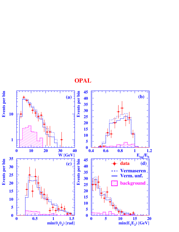
Figure 3: Comparison of the data with the Monte Carlo predictions for the EE sample. Shown are (a) the measured invariant mass, $W$, (b) the energy of the detected electron normalised to the energy of the beam electrons, $E_{\rm tag}$/$E_{\rm b}$, (c) the polar angle of the muon which is scattered closer to the beam direction, ${\rm min}(\theta_{1},\theta_{2})$, and (d) the energy of the muon with lower energy, ${\rm min}(E_{1},E_{2})$. The points represent the data with the statistical error only. The dashed lines denote the distributions of the Vermaseren Monte Carlo with the background added to it before the unfolding is performed, the full lines are the same distributions after reweighting based on the unfolding procedure, and the hatched histograms represent the background contribution

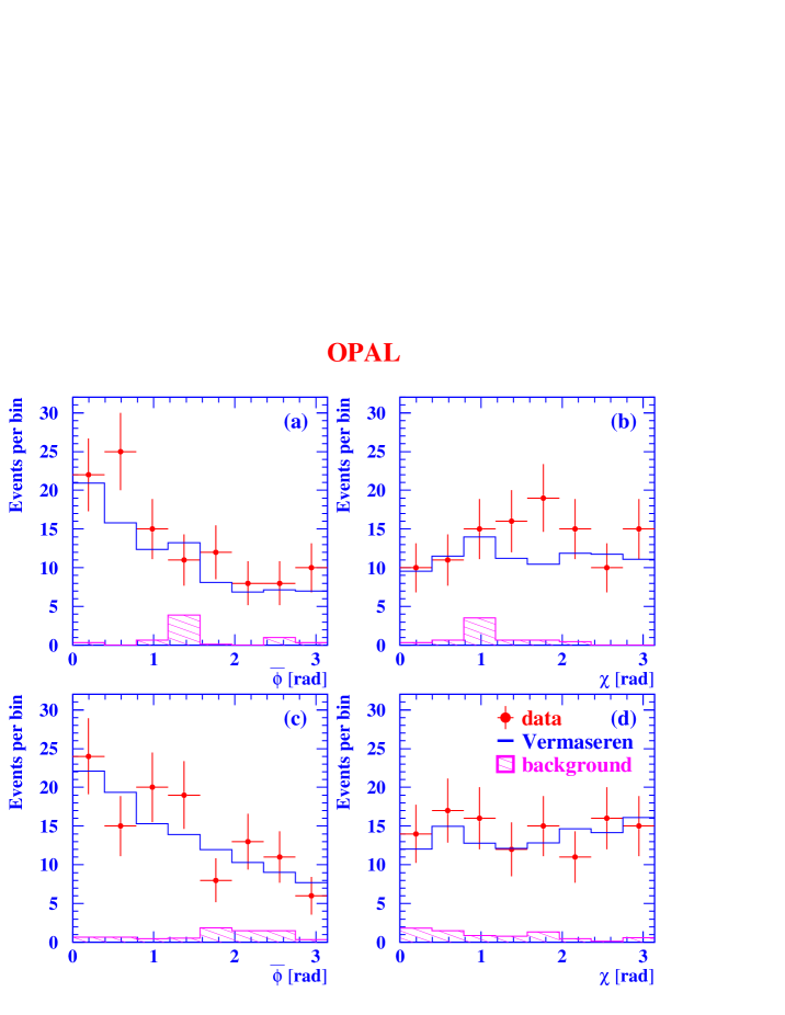
Figure 5: Comparison of the data with the Monte Carlo predictions for the DB samples. Figures (a,b) and (c,d) are for the DB1 and DB2 samples, respectively. Shown are (a,c) the angle $\bar{\phi}$ between the two scattering planes of the electrons in the photon-photon centre-of-mass system, and (b,d) the measured azimuthal angle, $\chi$, defined with respect to the plane containing the electron which radiated the photon of higher virtuality. The points represent the data with the statistical error only. The full lines denote the distributions of the Vermaseren Monte Carlo with the background added to it, and the hatched histograms represent the background contribution

For each of the samples, the agreement between the data and the Monte Carlo predictions, for signal and background events, is checked by comparing quantities reconstructed from the electrons and the muons. The variables used are the energies $E_{\rm tag}$, $E_{\rm stag}$, $E_{1}$, $E_{2}$, and angles $\theta_{\rm tag}$, $\theta_{\rm stag}$, $\theta_{1}$, $\theta_{2}$, of the detected electrons and of the first (1) and second (2) muon, and the derived quantities $y$, $Q^{2}$, $P^{2}$ and $W$. Good agreement of the distributions is found both in shape and normalisation for all samples. The agreement between the data and the Monte Carlo predictions of the SW and FD samples is similar to the findings of Ref. [7]. Some examples of control distributions for the EE sample and the DB samples are shown in Figures 3 and 4. The data with their statistical errors are compared to the signal Monte Carlo with the background added to it before the unfolding is performed, and to the Monte Carlo distributions after reweighting the signal events, where the weights are obtained from the unfolding procedure. All distributions show a good description of the data by the sum of signal and background Monte Carlo events. Figure 5 shows a comparison between the data and the Monte Carlo prediction for the DB samples before the unfolding using statistical errors only. Shown are the measured azimuthal angle $\bar{\phi}$ between the two scattering planes of the electrons in the photon-photon centre-of-mass system and the measured azimuthal angle, $\chi$, which, for doubly-tagged events, is defined with respect to the plane containing the electron which radiated the photon of higher virtuality. Both angular distributions of the data are well reproduceded by the Vermaseren program. The data exhibit a strong dependence on $\bar{\phi}$ which is well described by the prediction of Eq. 2. These distributions in principle give access to several other structure functions [12] but, due to the low statistics, no detailed analysis of these distributions has been performed.

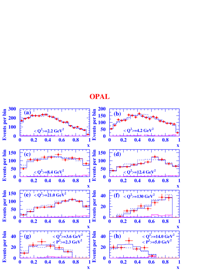
Figure 6: The measured $x$ distributions for the various samples (a) SW1, (b) SW2, (c) FD1, (d) FD2, (e) FD3, (f) EE, (g) DB1 and (h) DB2. The sample definitions are given in Table 1. The points represent the data with the statistical error only. The dashed lines denote the distributions of the Vermaseren Monte Carlo with the background added to it before the unfolding is performed, the full lines are the same distributions after reweighting based on the unfolding procedure, and the hatched histograms represent the background contribution

The differential cross-sections $\mathrm{d}\sigma/\mathrm{d}x$ and the structure functions $F_{\mathrm{2}}^{\gamma}$ are unfolded from the observed $x$ distribution of the data, shown in Figure 6. The distributions in Figure 6 are not corrected for radiative effects and trigger inefficiencies. Because the predicted $x$ distributions are close to the observed distributions, the results of the unfolding are also very close to the QED prediction. The method used to unfold the cross-section $\mathrm{d}\sigma/\mathrm{d}x$ and the structure function $F_{\mathrm{2}}^{\gamma}$ closely follows the procedure applied to the measurement of the hadronic structure function $F_{\mathrm{2,{\mathrm{h}ad}}}^{\gamma}$ and is described in detail in Ref. [26]. There is however a very important difference between the $\mu^{+}\mu^{-}$ final state and the hadronic final state. The resolution in $x$ of the $\mu^{+}\mu^{-}$ final state which, as determined form the signal Monte Carlo, amounts to about 0.03, is much better than the resolution in $x$ for the hadronic final state due to the good measurement of the invariant mass of the muon pair. Therefore a much finer binning in $x$ with much reduced correlations between the bins, could be chosen here.

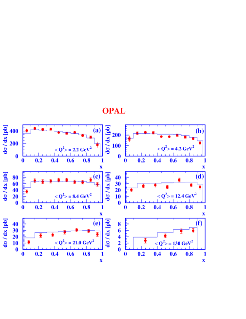
Figure 7: Differential cross-sections $\mathrm{d}\sigma/\mathrm{d}x$ unfolded from the data for the various independent samples of singly-tagged events. The samples shown are (a) SW1, (b) SW2, (c) FD1, (d) FD2, (e) FD3 and (f) EE. The points represent the data with their statistical (inner error bars) and total errors (outer error bars). The full line is the differential cross-sections as predicted by the Vermaseren Monte Carlo. The tic marks at the top of the figures indicate the bin boundaries

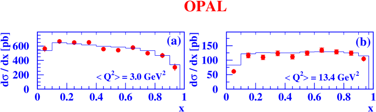
Figure 8: Differential cross-sections $\mathrm{d}\sigma/\mathrm{d}x$ unfolded from the data for the two combined samples of singly-tagged events. The samples shown are (a) SW and (b) FD. The symbols are as defined in Figure 7

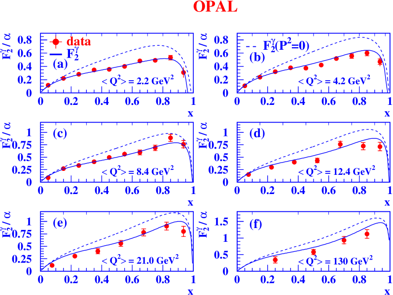
Figure 9: Structure functions $F_{\mathrm{2}}^{\gamma}$ normalised by the fine structure constant $\alpha$ for the various independent samples of singly-tagged events. The ordering of sub-figures is the same as in Figure 7. The points represent the data with their statistical (inner error bars) and total errors (outer error bars). The full line is the structure function $F_{\mathrm{2}}^{\gamma}$ normalised by the fine structure constant $\alpha$ for the $\langle Q^{2}\rangle$ and $\langle P^{2}\rangle$ values listed in Table 1, and the dashed line shows the structure function $F_{\mathrm{2}}^{\gamma}$ normalised by the fine structure constant $\alpha$ for the same $\langle Q^{2}\rangle$ but for $P^{2}=0$. The tic marks at the top of the figures indicate the bin boundaries

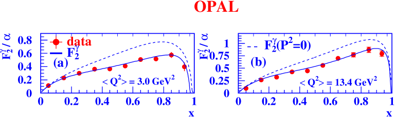
Figure 10: Structure functions $F_{\mathrm{2}}^{\gamma}$ normalised by the fine structure constant $\alpha$ for the two combined samples of singly-tagged events. The samples shown are (a) SW and (b) FD. The symbols are as defined in Figure 9

The differential cross-sections $\mathrm{d}\sigma/\mathrm{d}x$ and the structure functions $F_{\mathrm{2}}^{\gamma}$, normalised by the fine structure constant $\alpha$, unfolded from the data, are shown in Figure 7 and Figure 9 for the independent samples of singly-tagged events and in Figure 8 and Figure 10 for the combined SW and FD samples. The measured values are corrected both for radiative effects and for the trigger inefficiencies. The radiative corrections are based on the ratio of the predicted cross-sections by the BDK and Vermaseren programs in bins of $x$. The radiative corrections vary with $Q^{2}$ and $x$ and amount up to about $\pm 9\%$. The structure function values are given at the centres of the $x$ bins. Because, in a given bin in $x$, the average value of $F_{\mathrm{2}}^{\gamma}$ is different from the value of $F_{\mathrm{2}}^{\gamma}$ at the centre of the $x$ bin, the results has to be corrected for this bin size effect. The measured average value of $F_{\mathrm{2}}^{\gamma}$ in a given bin in $x$, as obtained from the unfolding, is corrected for the bin size effect by multiplying the measured value of $F_{\mathrm{2}}^{\gamma}$ with the QED prediction of the ratio of $F_{\mathrm{2}}^{\gamma}$ at the centre of the bin and the average $F_{\mathrm{2}}^{\gamma}$ in the bin. In general the corrections are small and the largest corrections occur at low, and high values of $x$. The corrections are below 1$\%$ in all but the lowest and highest bins in $x$, for all samples. In the lowest and highest bins in $x$ the correction is always positive, and amounts up to 7$\%$ in the lowest $x$ bins, and in the highest $x$ bins it is around 5$\%$, with the exception of the SW1 sample, where it is largest and amounts to 19$\%$. The vertical error bars show both the statistical error and the full error, which is obtained from the quadratic sum of statistical and systematic errors. In all unfolded results, the statistical error is obtained from the quadratic sum of the statistical error of the data events and the signal Monte Carlo events. The measured values for the cross-sections $\mathrm{d}\sigma/\mathrm{d}x$ are listed in Tables 2$-$5 and the structure functions in Tables 6$-$8. For the cross-section measurement of the singly-tagged events, the corrected data correspond to the phase space defined by $y<0.5$, $P^{2}<1.4$ $\rm GeV^{2}$ and the $Q^{2}$ ranges listed in Table 1. The full range of $W$ is used, except for the EE sample where $W^{2}>1$ $\rm GeV^{2}$ is required. For the doubly-tagged events, the corrected data correspond to the phase space defined by $y<0.5$ and the $Q^{2}$ and $P^{2}$ ranges listed in Table 1.

The systematic error receives contributions from several sources. The determination of $x$ and $Q^{2}$ is based on the measurement of the muon and electron momenta. The uncertainties in these measurements are taken into account by shifting the reconstructed quantities in the Monte Carlo samples according to resolution and repeating the unfolding. The variations performed are the following.

• The transverse momentum of the muons is shifted by 0.25$\%$ for tracks in the region $|\cos\theta_{\mu}|<0.90$ and by 5$\%$ for very forward tracks, which are less well measured up to $|\cos\theta_{\mu}|=0.96$.

• The polar angle and the azimuthal angle of the muons are shifted by 0.2 mrad for tracks in the region $|\cos\theta_{\mu}|<0.90$ and by 1 mrad for very forward tracks up to $|\cos\theta_{\mu}|=0.96$.

• The polar angle of the observed electron is shifted by 0.3 mrad, 0.7 mrad and 5 mrad for electrons observed in the SW, FD and EE calorimeters, respectively.

The differences of the results based on the central values and the results obtained using the shifted values are added in quadrature. The systematic errors due to the uncertainties in the determination of trigger efficiencies and of the radiative corrections are also added in quadrature. The uncertainty is dominated in almost all bins by the statistical error.

The predicted structure function $F_{\mathrm{2}}^{\gamma}$ is strongly suppressed for $P^{2}=\langle P^{2}\rangle$ compared to $P^{2}=0$. The measured structure functions Figures 9 and 10 are distinctly different from the predictions for $P^{2}=0$ for all values of $Q^{2}$. In general there is good agreement between the data and the predictions for all ranges in $Q^{2}$, and the corresponding $\chi^{2}$ probabilities $P(\chi^{2})$ are listed in Tables 2$-$8. Some small differences between the data and the predictions can be seen for $Q^{2}>10$ $\rm GeV^{2}$. For the individual FD samples, FD2 and FD3, the data shows a slightly different shape for $x<0.5$ than the predicted differential cross section, Figure 7(d,e), and the structure function, Figure 9(d,e), and for the EE sample the predicted differential cross section, Figure 7(f), and the structure function Figure 9(f), are slightly higher than what is observed in the data for all $x$.

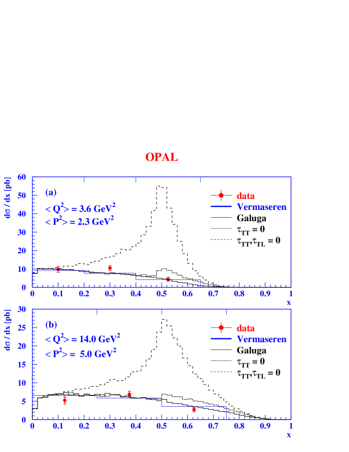
Figure 11: Differential cross-sections $\mathrm{d}\sigma/\mathrm{d}x$ unfolded from the data, (a) for the DB1 sample and (b) for the DB2 sample. The sample definitions are given in Table 1. The points represent the data with their statistical (inner error bars) and total errors (outer error bars). The full line denotes the differential cross-sections as predicted by the Vermaseren Monte Carlo using the same bins as for the data. The additional three histograms represent the cross-section calculations from the GALUGA Monte Carlo for three different scenarios: the full cross-section (full line), the cross-section obtained for vanishing $\tau_{\mathrm{TT}}$ (dot-dash) and the cross-section obtained for vanishing $\tau_{\mathrm{TT}}$ and $\tau_{\mathrm{TL}}$ (dash), as defined in Eq. 2. The tic marks at the top of the figures indicate the bin boundaries

The cross-sections for the samples DB1 and DB2, unfolded from the data, are listed in Table 5 and shown in Figure 11, together with the predictions from the Vermaseren and GALUGA programs. The data are well described by both Monte Carlos using the full cross-section from Eq. 2. Using the GALUGA predictions, the influence of the non-vanishing terms proportional to $\cos\bar{\phi}$ and $\cos 2\bar{\phi}$ can be seen. If these terms are neglected, the predicted cross-section grossly overestimates the measured cross-section. This shows that both terms, $\tau_{\mathrm{TT}}$ and $\tau_{\mathrm{TL}}$, are present, mainly at $x>0.1$, and that the corresponding contributions to the cross-section are negative. The contribution from $\tau_{\mathrm{TL}}$ is especially very large in the specific kinematical region of the DB samples. There is also good agreement between the number of events predicted and observed for the DB3 sample but, because of its low statistics, no cross-section is evaluated for that sample.

6 Results for $\bf F_{\mathrm{A}}^{\gamma}$ and $\bf F_{\mathrm{B}}^{\gamma}$

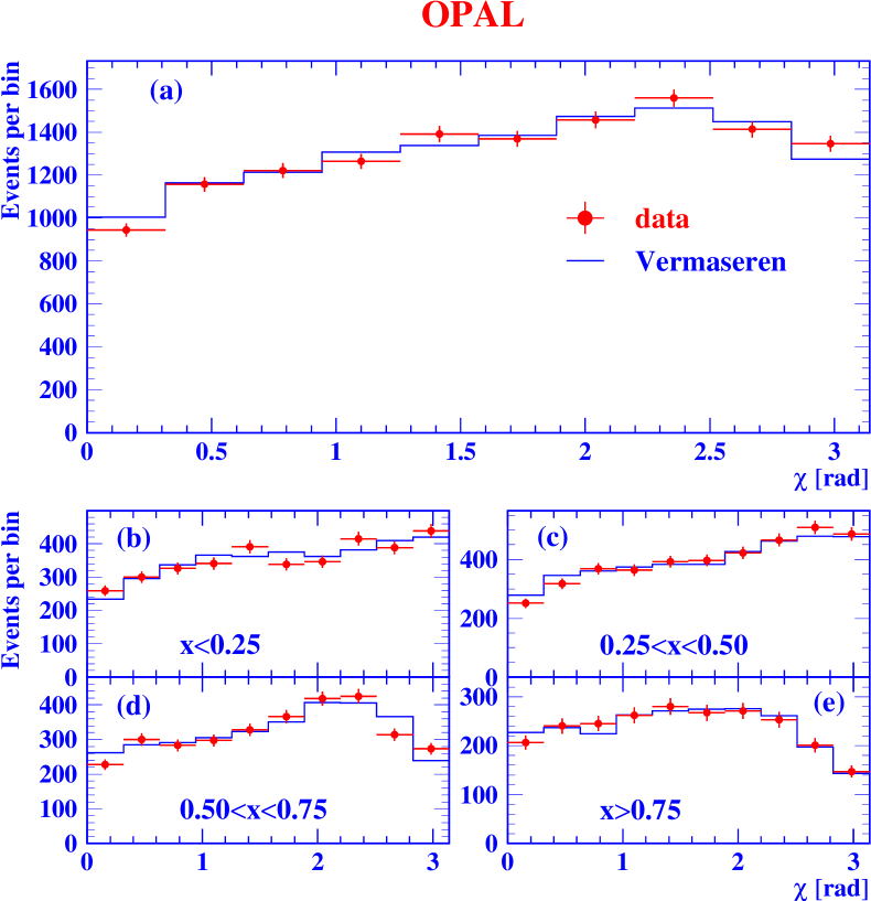
Figure 12: Measured azimuthal angle distributions for the combined SW and FD sample for different ranges in $x$. The points represent the data with the statistical error only, and the full line is the prediction of the Vermaseren Monte Carlo normalised to the number of events in the data

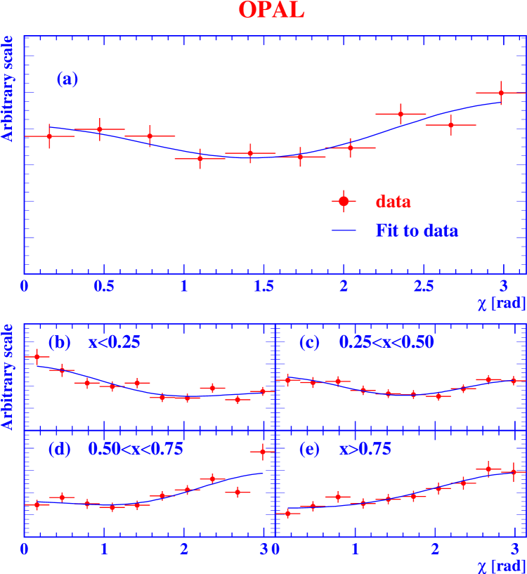
Figure 13: Corrected azimuthal angle distributions for the combined SW and FD sample for different ranges of $x$. The points represent the corrected data with the statistical error only, and the full line is a fit to the data based on Eq. 13

For the combined SW and FD samples, the quantities $F_{\mathrm{A}}^{\gamma}/F_{\mathrm{2}}^{\gamma}$ and $\frac{1}{2}F_{\mathrm{B}}^{\gamma}/F_{\mathrm{2}}^{\gamma}$ are obtained in bins of $x$ from the azimuthal angle distributions shown in Figure 12. The resolution in $\chi$ is about 20 mrad over the whole range of $\chi$. The measured distributions do not exhibit directly the $\cos\chi$ and $\cos 2\chi$ dependences predicted by QED in Eq. 7. This is mainly due to the loss of muons close to the beam axis in the region $|\cos\theta_{\mu}|>0.96$. In order to extract $F_{\mathrm{A}}^{\gamma}/F_{\mathrm{2}}^{\gamma}$ and $\frac{1}{2}F_{\mathrm{B}}^{\gamma}/F_{\mathrm{2}}^{\gamma}$, the azimuthal angle distributions are corrected for this and other detector effects using a bin-by-bin correction in $\chi$ for ranges of $x$. The correction factor is a given bin is obtained from the distribution of the generated $\chi$ for events passing the selection cuts, where each event is weighted by $1/(1+F_{\mathrm{A}}^{\gamma}/F_{\mathrm{2}}^{\gamma}\cos\chi+\frac{1}{2}F_{\mathrm{B}}^{\gamma}/F_{\mathrm{2}}^{\gamma}\cos 2\chi)$. The ratios $F_{\mathrm{A}}^{\gamma}/F_{\mathrm{2}}^{\gamma}$ and $F_{\mathrm{B}}^{\gamma}/F_{\mathrm{2}}^{\gamma}$ used in the weighting function are determined from the analytical QED structure functions Eq’s. 8$-$10. The weighted distribution is equivalent to what would be obtained from a flat $\chi$ distribution. The corrected distributions are shown in Figure 13. They are fitted to the following function:

$$F(\chi)=A(1+B\cos\chi+C\cos 2\chi),$$ (13)

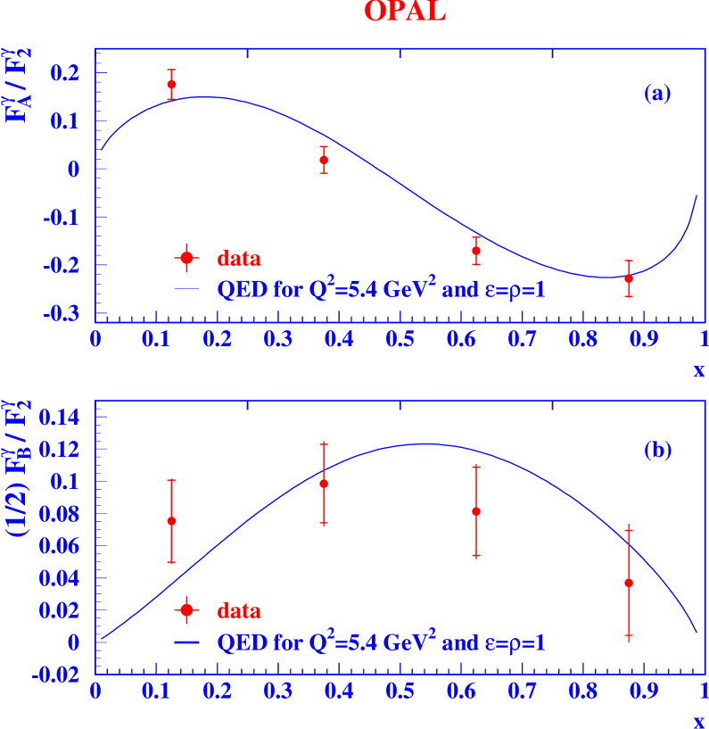
Figure 14: The measured structure function ratios $F_{\mathrm{A}}^{\gamma}/F_{\mathrm{2}}^{\gamma}$ and $\frac{1}{2}F_{\mathrm{B}}^{\gamma}/F_{\mathrm{2}}^{\gamma}$ for the combined SW and FD sample. The points represent the data with their statistical (inner error bars) and total errors (outer error bars). The solid lines are the QED predictions for $Q^{2}=5.4$ $\rm GeV^{2}$ and $\epsilon=\rho=1$. $\chi^{2}/{\rm dof}=5.9/4$ for $F_{\mathrm{A}}^{\gamma}/F_{\mathrm{2}}^{\gamma}$ and $\chi^{2}/{\rm dof}=4.4/4$ for $\frac{1}{2}F_{\mathrm{B}}^{\gamma}/F_{\mathrm{2}}^{\gamma}$

where $A$ is a normalisation factor, which is left free in the fit, $B=F_{\mathrm{A}}^{\gamma}/F_{\mathrm{2}}^{\gamma}$, and $C=\frac{1}{2}F_{\mathrm{B}}^{\gamma}/F_{\mathrm{2}}^{\gamma}$, for $\epsilon=\rho=1$. The correlation coefficients between the parameters $B$ and $C$ resulting from the fits are $0.04$ over the whole $x$ range and $0.26$, $0.13$, $-0.11$ and $-0.29$ for the different bins in $x$, as given in Table 9. The measured average values of $F_{\mathrm{A}}^{\gamma}/F_{\mathrm{2}}^{\gamma}$ and $\frac{1}{2}F_{\mathrm{B}}^{\gamma}/F_{\mathrm{2}}^{\gamma}$ in bins of $x$, as obtained from the fit, are corrected for the bin size effect as before. The measured values of $\frac{1}{2}F_{\mathrm{B}}^{\gamma}/F_{\mathrm{2}}^{\gamma}$ are in good agreement with the previous OPAL measurement of $\frac{1}{2}F_{\mathrm{B}}^{\gamma}/F_{\mathrm{2}}^{\gamma}$ [7]. The corrected values of $F_{\mathrm{A}}^{\gamma}/F_{\mathrm{2}}^{\gamma}$ and $\frac{1}{2}F_{\mathrm{B}}^{\gamma}/F_{\mathrm{2}}^{\gamma}$ are listed in Table 9 and shown in Figure 14 compared to the QED predictions for $Q^{2}=5.4$ $\rm GeV^{2}$ and $\epsilon=\rho=1$. The QED predictions for the full range in $x$ of $F_{\mathrm{A}}^{\gamma}/F_{\mathrm{2}}^{\gamma}=-0.027$ and $\frac{1}{2}F_{\mathrm{B}}^{\gamma}/F_{\mathrm{2}}^{\gamma}=0.078$ are in good agreement with the measured values, $F_{\mathrm{A}}^{\gamma}/F_{\mathrm{2}}^{\gamma}=-0.036\pm 0.027\pm 0.004$ and $\frac{1}{2}F_{\mathrm{B}}^{\gamma}/F_{\mathrm{2}}^{\gamma}=0.061\pm 0.013\pm 0.004$. The measured values of $\frac{1}{2}F_{\mathrm{B}}^{\gamma}/F_{\mathrm{2}}^{\gamma}$ as a function of $x$ are significantly different from zero and the measured shape agrees with the QED prediction, although it is not significantly different from a constant.

The sources of systematic errors are

• Detector effects:
  The same variations as carried out for the measurement of $F_{\mathrm{2}}^{\gamma}$ and $\mathrm{d}\sigma/\mathrm{d}x$ and described in Section 5, have been performed.

• Reweighting procedure:
  The reweighting procedure is tested by using a version of the TWOGEN [27] generator where the structure functions $F_{\mathrm{A}}^{\gamma}$ and $F_{\mathrm{B}}^{\gamma}$ can be chosen arbitrarily. By chosing one of the two structure functions to be a constant and measuring the other structure function, systematic uncertainties varying between 0.03$\%$ and 3.3$\%$ for the measurement of $F_{\mathrm{A}}^{\gamma}/F_{\mathrm{2}}^{\gamma}$ and between 0.7$\%$ and 3.8$\%$ for $\frac{1}{2}F_{\mathrm{B}}^{\gamma}/F_{\mathrm{2}}^{\gamma}$ in the different $x$ ranges are found.

• Background:
  As the background is not subtracted from the data, the fit to the data is a superposition of the fit to the signal and background distributions contributing with their relative fractions. To take the effect of the background distribution into account in the estimation of the systematic error, the $\chi$ distribution of the background is corrected, using the same procedure as for the data, and then fitted like the data. The parameters $B$ and $C$ of this fit are weighted by the relative contribution of the background to the data for each range in $x$. They constitute the estimate of the systematic error, which varies from 1.4$\%$ to 4.2$\%$ between the low and high $x$ range.

The strength of the $\chi$ dependence varies with the scattering angle $\cos\theta^{\star}$ of the muons in the photon-photon centre-of-mass system. Reducing the acceptance of $\cos\theta^{\star}$ enhances the $\chi$ dependence but, to obtain a result for $F_{\mathrm{A}}^{\gamma}$ and $F_{\mathrm{B}}^{\gamma}$ which is valid for the full range of $\cos\theta^{\star}$ the measurement has to be extrapolated using the predictions of QED. The measurements of Ref. [6] are obtained in the range $|\cos\theta^{\star}|<0.7$, and extrapolated to the full range in $\cos\theta^{\star}$, whereas the measurement presented here is valid for the full angular range $|\cos\theta^{\star}|<1$. Taking this into account, the results for $F_{\mathrm{A}}^{\gamma}/F_{\mathrm{2}}^{\gamma}$ and $\frac{1}{2}F_{\mathrm{B}}^{\gamma}/F_{\mathrm{2}}^{\gamma}$ obtained here and the measurements of Ref. [6] are consistent.

From the measurements of $F_{\mathrm{A}}^{\gamma}/F_{\mathrm{2}}^{\gamma}$ and $\frac{1}{2}F_{\mathrm{B}}^{\gamma}/F_{\mathrm{2}}^{\gamma}$ and $F_{\mathrm{2}}^{\gamma}$, the values of $F_{\mathrm{A}}^{\gamma}$ and $F_{\mathrm{B}}^{\gamma}$ are obtained in the following way. The data from the SW and FD sample are combined and the structure function $F_{\mathrm{2}}^{\gamma}$ is unfolded using the same bins as those used for the measurement of $F_{\mathrm{A}}^{\gamma}/F_{\mathrm{2}}^{\gamma}$ and $\frac{1}{2}F_{\mathrm{B}}^{\gamma}/F_{\mathrm{2}}^{\gamma}$. As Eq’s. 8$-$10, used for the measurement of $F_{\mathrm{A}}^{\gamma}/F_{\mathrm{2}}^{\gamma}$ and $\frac{1}{2}F_{\mathrm{B}}^{\gamma}/F_{\mathrm{2}}^{\gamma}$, are only valid for $P^{2}=0$, the measurement of $F_{\mathrm{2}}^{\gamma}$ is corrected for the effect of non-zero $P^{2}$ in the data by multiplying the result of the unfolding for $\langle P^{2}\rangle=0.05$ $\rm GeV^{2}$ by the ratio of $F_{\mathrm{2}}^{\gamma}$ for $P^{2}=0$ and $F_{\mathrm{2}}^{\gamma}$ for $\langle P^{2}\rangle=0.05$ $\rm GeV^{2}$ as predicted by QED. Then $F_{\mathrm{A}}^{\gamma}$ and $F_{\mathrm{B}}^{\gamma}$ are calculated by multiplying the measured ratios by $F_{\mathrm{2}}^{\gamma}$ and corrected for the bin size effect as before. The corrected values for $F_{\mathrm{2}}^{\gamma}$, $F_{\mathrm{A}}^{\gamma}$ and $F_{\mathrm{B}}^{\gamma}$ are listed in Table 10, and $F_{\mathrm{A}}^{\gamma}$ and $F_{\mathrm{B}}^{\gamma}$ are shown in Figure 15. The QED predictions for $Q^{2}$ = 5.4 $\rm GeV^{2}$ and $\epsilon=\rho=1$ nicely describe the data.

7 Summary and conclusions

The complete set of data collected by the OPAL experiment at centre-of-mass energies close to the mass of the $\rm Z$ boson are used to extract information about the QED structure of the photon. The structure function $F_{\mathrm{2}}^{\gamma}$ and the differential cross-section $\mathrm{d}\sigma/\mathrm{d}x$ for quasi-real photons are measured in the $Q^{2}$ range from 1.5 to 400 $\rm GeV^{2}$, the largest kinematic range ever covered by a single experiment. The predictions of QED are found to be in good agreement with the data, and the predicted $P^{2}$ suppression of the structure function $F_{\mathrm{2}}^{\gamma}$ is clearly observed.

For the first time, the detailed quantitative analysis of the QED structure of the photon has been extended to highly virtual photons. Due to the non-vanishing interference terms $\tau_{\mathrm{TL}}$ and $\tau_{\mathrm{TT}}$ in the kinematical region studied, strong cancellations in the differential cross-section occur between the cross-section and interference terms. Consequently, no clear relation of a structure function to the cross-section terms can be found. Therefore the differential cross-section for the reaction $\rm ee\rightarrow\rm ee\mu^{+}\mu^{-}$, proceeding via the exchange of two highly virtual photons is measured instead, for the range $1.5<Q^{2}<30$ $\rm GeV^{2}$ and $1.5<P^{2}<20$ $\rm GeV^{2}$. The QED predictions using the GALUGA program show good agreement with the data for the full cross-section and also the presence of the interference terms $\tau_{\mathrm{TL}}$ and $\tau_{\mathrm{TT}}$ in the data.

The azimuthal correlations between electrons and muons are used to extract the structure functions $F_{\mathrm{A}}^{\gamma}$ and $F_{\mathrm{B}}^{\gamma}$ in bins of $x$. The results are consistent with those already published and with the QED predictions. The measurements presented here supersede the earlier structure function results of OPAL [7, 4]

Acknowledgements:

We wish to thank C. Berger and G. Schuler for valuable discussions concerning the interpretation of the measurements for highly virtual photons and M. Seymour for providing us with the structure function calculations for the measurement of $F_{\mathrm{A}}^{\gamma}$ and $F_{\mathrm{B}}^{\gamma}$.

We particularly wish to thank the SL Division for the efficient operation of the LEP accelerator at all energies and for their continuing close cooperation with our experimental group. We thank our colleagues from CEA, DAPNIA/SPP, CE-Saclay for their efforts over the years on the time-of-flight and trigger systems which we continue to use. In addition to the support staff at our own institutions we are pleased to acknowledge the
Department of Energy, USA,
National Science Foundation, USA,
Particle Physics and Astronomy Research Council, UK,
Natural Sciences and Engineering Research Council, Canada,
Israel Science Foundation, administered by the Israel Academy of Science and Humanities,
Minerva Gesellschaft,
Benoziyo Center for High Energy Physics,
Japanese Ministry of Education, Science and Culture (the Monbusho) and a grant under the Monbusho International Science Research Program,
Japanese Society for the Promotion of Science (JSPS),
German Israeli Bi-national Science Foundation (GIF),
Bundesministerium für Bildung, Wissenschaft, Forschung und Technologie, Germany,
National Research Council of Canada,
Research Corporation, USA,
Hungarian Foundation for Scientific Research, OTKA T-016660, T023793 and OTKA F-023259.

Sample	SW1	SW2	SW
$Q^{2}$ [$\rm GeV^{2}$ ]	1.5$-$3	3$-$7	1.5$-$7
$P^{2}$ [$\rm GeV^{2}$ ]	$-$	$-$	$-$
$x$	0$-$0.97	0$-$0.97	0$-$0.97
$y$	0$-$0.5	0$-$0.5	0$-$0.5
$\langle Q^{2}\rangle$ [$\rm GeV^{2}$ ]	2.2	4.2	3.0
$\langle P^{2}\rangle$ [$\rm GeV^{2}$ ]	0.05	0.05	0.05
data	3259 $\pm$ 57	2292 $\pm$ 48	5551 $\pm$ 75
signal	3176 $\pm$ 25	2273 $\pm$ 21	5449 $\pm$ 33
background	47.9 $\pm$ 6.7	60.6 $\pm$ 9.2	108.6 $\pm$ 11.4
Sample	FD1	FD2	FD3	FD
$Q^{2}$ [$\rm GeV^{2}$ ]	6$-$10	10$-$15	15$-$30	6$-$30
$P^{2}$ [$\rm GeV^{2}$ ]	$-$	$-$	$-$	$-$
$x$	0$-$0.97	0$-$0.97	0$-$0.97	0$-$0.97
$y$	0$-$0.5	0$-$0.5	0$-$0.5	0$-$0.5
$\langle Q^{2}\rangle$ [$\rm GeV^{2}$ ]	8.4	12.4	21.0	13.4
$\langle P^{2}\rangle$ [$\rm GeV^{2}$ ]	0.05	0.05	0.05	0.05
data	1058 $\pm$ 33	790 $\pm$ 28	719 $\pm$ 27	2567 $\pm$ 51
signal	988 $\pm$ 16	803 $\pm$ 14	738 $\pm$ 13	2531 $\pm$ 25
background	41.4 $\pm$ 4.0	39.5 $\pm$ 3.9	38.2 $\pm$ 3.9	119.1 $\pm$ 6.8
Sample	EE	DB1	DB2	DB3
$Q^{2}$ [$\rm GeV^{2}$ ]	70$-$400	1.5$-$6	6$-$30	70$-$300
$P^{2}$ [$\rm GeV^{2}$ ]	$-$	1.5$-$6	1.5$-$20	1.5$-$20
$x$	0.1$-$0.9	0$-$0.65	0$-$0.75	0$-$1
$y$	0$-$0.5	0$-$0.5	0$-$0.5	0$-$0.5
$\langle Q^{2}\rangle$ [$\rm GeV^{2}$ ]	130	3.6	14.0	140
$\langle P^{2}\rangle$ [$\rm GeV^{2}$ ]	0.05	2.3	5.0	16
data	163 $\pm$ 12.8	111 $\pm$ 10.5	116 $\pm$ 10.8	8 $\pm$ 2.8
signal	161.9 $\pm$ 4.7	85.0 $\pm$ 2.5	102.1 $\pm$ 2.7	7.9 $\pm$ 0.8
background	17.4 $\pm$ 2.7	6.4 $\pm$ 3.1	7.5 $\pm$ 1.4	2.0 $\pm$ 0.7

Table 1: The sample definitions in terms of $P^{2}$, $Q^{2}$, $x$ and $y$, the average values $\langle Q^{2}\rangle$ and $\langle P^{2}\rangle$ as obtained from the data and Monte Carlo and the number of events selected from the data (data), together with the predictions of the signal Monte Carlo (signal) and background events (background). The SW and the FD samples are not statistically independent from the other samples, i.e. the SW sample contains all events from SW1 and SW2 and the FD sample contains all events from FD1, FD2 and FD3

	SW1	SW2	SW
$x$	$\mathrm{d}\sigma/\mathrm{d}x$ [pb]	$\mathrm{d}\sigma/\mathrm{d}x$ [pb]	$\mathrm{d}\sigma/\mathrm{d}x$ [pb]
0.00$-$0.10	409.0 $\pm$ 23.6 $\pm$ 16.3	164.4 $\pm$ 15.0 $\pm$ 25.0	562.3 $\pm$ 28.3 $\pm$ 33.2
0.10$-$0.20	443.4 $\pm$ 19.7 $\pm$ 16.7	217.4 $\pm$ 13.0 $\pm$   8.2	663.0 $\pm$ 25.4 $\pm$ 22.3
0.20$-$0.30	423.2 $\pm$ 18.8 $\pm$ 16.2	223.8 $\pm$ 12.3 $\pm$   8.2	647.9 $\pm$ 24.4 $\pm$ 22.4
0.30$-$0.40	430.9 $\pm$ 18.3 $\pm$ 13.8	220.9 $\pm$ 11.8 $\pm$   6.6	650.3 $\pm$ 23.6 $\pm$ 21.4
0.40$-$0.50	377.7 $\pm$ 17.6 $\pm$ 10.9	185.7 $\pm$ 10.1 $\pm$   4.9	556.3 $\pm$ 21.6 $\pm$ 12.5
0.50$-$0.60	366.0 $\pm$ 18.3 $\pm$ 10.3	184.8 $\pm$ 10.8 $\pm$   5.5	542.4 $\pm$ 22.6 $\pm$ 15.0
0.60$-$0.70	380.1 $\pm$ 19.9 $\pm$ 12.4	198.3 $\pm$ 11.1 $\pm$   4.9	578.7 $\pm$ 24.3 $\pm$ 23.4
0.70$-$0.80	329.5 $\pm$ 20.6 $\pm$   7.8	181.0 $\pm$ 11.1 $\pm$   3.6	500.9 $\pm$ 24.3 $\pm$ 12.3
0.80$-$0.90	302.5 $\pm$ 19.4 $\pm$   7.4	166.7 $\pm$ 11.1 $\pm$   3.6	467.7 $\pm$ 23.9 $\pm$ 28.0
0.90$-$0.97	181.6 $\pm$ 18.7 $\pm$ 41.9	124.3 $\pm$ 11.0 $\pm$ 13.5	304.9 $\pm$ 22.3 $\pm$ 45.5
$\langle Q^{2}\rangle$	2.2 $\rm GeV^{2}$	4.2 $\rm GeV^{2}$	3.0 $\rm GeV^{2}$
$P(\chi^{2})$	0.79	0.26	0.46

Table 2: The measured differential cross-section $\mathrm{d}\sigma/\mathrm{d}x$ for the SW samples. In addition, the average $Q^{2}$ value for each sample, $\langle Q^{2}\rangle$, and the $\chi^{2}$ probabilities, $P(\chi^{2})$, are listed. The sample definitions are given in Table 1. The SW sample contains all events from SW1 and SW2. The first error is statistical and the second systematic

	FD1	FD
$x$	$\mathrm{d}\sigma/\mathrm{d}x$ [pb]	$\mathrm{d}\sigma/\mathrm{d}x$ [pb]
0.00$-$0.10	35.4 $\pm$ 4.8 $\pm$ 2.8	61.2 $\pm$ 6.7 $\pm$ 4.2
0.10$-$0.20	69.4 $\pm$ 5.6 $\pm$ 4.9	116.2 $\pm$ 8.1 $\pm$ 6.0
0.20$-$0.30	66.2 $\pm$ 5.8 $\pm$ 4.0	109.6 $\pm$ 7.9 $\pm$ 5.0
0.30$-$0.40	67.9 $\pm$ 5.5 $\pm$ 3.6	123.2 $\pm$ 8.1 $\pm$ 5.7
0.40$-$0.50	71.2 $\pm$ 5.5 $\pm$ 3.8	111.5 $\pm$ 7.5 $\pm$ 4.4
0.50$-$0.60	71.3 $\pm$ 5.4 $\pm$ 3.3	124.2 $\pm$ 7.5 $\pm$ 5.1
0.60$-$0.70	65.3 $\pm$ 5.4 $\pm$ 2.5	134.5 $\pm$ 7.7 $\pm$ 5.7
0.70$-$0.80	64.8 $\pm$ 5.3 $\pm$ 2.2	128.3 $\pm$ 7.4 $\pm$ 4.3
0.80$-$0.90	72.1 $\pm$ 5.8 $\pm$ 3.5	124.2 $\pm$ 7.6 $\pm$ 4.8
0.90$-$0.97	57.5 $\pm$ 5.6 $\pm$ 3.7	104.6 $\pm$ 7.0 $\pm$ 5.8
$\langle Q^{2}\rangle$	8.4 $\rm GeV^{2}$	13.4 $\rm GeV^{2}$
$P(\chi^{2})$	0.61	0.13

	FD2	FD3
$x$	$\mathrm{d}\sigma/\mathrm{d}x$ [pb]	$\mathrm{d}\sigma/\mathrm{d}x$ [pb]
0.00$-$0.15	20.2 $\pm$ 2.9 $\pm$ 1.6	11.5 $\pm$ 2.7 $\pm$ 1.2
0.15$-$0.30	26.4 $\pm$ 3.0 $\pm$ 1.5	21.9 $\pm$ 2.8 $\pm$ 1.5
0.30$-$0.45	27.6 $\pm$ 2.8 $\pm$ 1.7	22.9 $\pm$ 2.9 $\pm$ 1.6
0.45$-$0.60	24.7 $\pm$ 2.5 $\pm$ 1.9	26.9 $\pm$ 2.8 $\pm$ 1.4
0.60$-$0.75	35.7 $\pm$ 2.9 $\pm$ 1.9	30.5 $\pm$ 2.7 $\pm$ 1.3
0.75$-$0.90	27.9 $\pm$ 2.8 $\pm$ 1.1	28.9 $\pm$ 2.5 $\pm$ 1.1
0.90$-$0.97	24.5 $\pm$ 2.9 $\pm$ 1.0	23.6 $\pm$ 3.0 $\pm$ 1.0
$\langle Q^{2}\rangle$	12.4 $\rm GeV^{2}$	21.0 $\rm GeV^{2}$
$P(\chi^{2})$	0.07	0.09

Table 3: The differential cross-section $\mathrm{d}\sigma/\mathrm{d}x$ for the FD samples. In addition, the average $Q^{2}$ value for each sample, $\langle Q^{2}\rangle$, and the $\chi^{2}$ probabilities, $P(\chi^{2})$, are listed. The sample definitions are given in Table 1. The FD sample contains all events from FD1, FD2 and FD3. The first error is statistical and the second systematic

	EE
$x$	$\mathrm{d}\sigma/\mathrm{d}x$ [pb]
0.1$-$0.4	2.78 $\pm$ 0.76 $\pm$ 0.28
0.4$-$0.6	4.27 $\pm$ 0.58 $\pm$ 0.38
0.6$-$0.8	5.79 $\pm$ 0.67 $\pm$ 0.39
0.8$-$0.9	5.88 $\pm$ 0.68 $\pm$ 0.30
$\langle Q^{2}\rangle$	130 $\rm GeV^{2}$
$P(\chi^{2})$	0.48

Table 4: The measured differential cross-section $\mathrm{d}\sigma/\mathrm{d}x$ for the EE sample. In addition, the average $Q^{2}$ value for the sample, $\langle Q^{2}\rangle$, and the $\chi^{2}$ probability, $P(\chi^{2})$, are listed. The sample definition is given in Table 1. The first error is statistical and the second systematic

	DB1		DB2
$x$	$\mathrm{d}\sigma/\mathrm{d}x$ [pb]	$x$	$\mathrm{d}\sigma/\mathrm{d}x$ [pb]
0.00$-$0.20	9.77 $\pm$ 1.62 $\pm$ 0.78	0.00$-$0.25	5.26 $\pm$ 0.82 $\pm$ 0.99
0.20$-$0.40	10.45 $\pm$ 1.26 $\pm$ 0.59	0.25$-$0.50	6.87 $\pm$ 0.78 $\pm$ 0.74
0.40$-$0.65	4.34 $\pm$ 1.07 $\pm$ 0.21	0.50$-$0.75	2.75 $\pm$ 0.60 $\pm$ 0.22
$\langle Q^{2}\rangle$	3.6 $\rm GeV^{2}$	$\langle Q^{2}\rangle$	14.0 $\rm GeV^{2}$
$\langle P^{2}\rangle$	2.3 $\rm GeV^{2}$	$\langle P^{2}\rangle$	5.0 $\rm GeV^{2}$
$P(\chi^{2})$	0.26	$P(\chi^{2})$	0.32

Table 5: The measured differential cross-section $\mathrm{d}\sigma/\mathrm{d}x$ for the DB samples. In addition, the average $Q^{2}$ and $P^{2}$ values for each sample, $\langle Q^{2}\rangle$ and $\langle P^{2}\rangle$, and the $\chi^{2}$ probabilities, $P(\chi^{2})$, are listed. The sample definitions are given in Table 1. The first error is statistical and the second systematic

	SW1	SW2	SW
$x$	$F_{\mathrm{2}}^{\gamma}$	$F_{\mathrm{2}}^{\gamma}$	$F_{\mathrm{2}}^{\gamma}$
0.00$-$0.10	0.115 $\pm$ 0.007 $\pm$ 0.005	0.108 $\pm$ 0.010 $\pm$ 0.016	0.113 $\pm$ 0.006 $\pm$ 0.007
0.10$-$0.20	0.219 $\pm$ 0.010 $\pm$ 0.008	0.237 $\pm$ 0.014 $\pm$ 0.009	0.230 $\pm$ 0.009 $\pm$ 0.008
0.20$-$0.30	0.282 $\pm$ 0.012 $\pm$ 0.011	0.320 $\pm$ 0.018 $\pm$ 0.012	0.300 $\pm$ 0.011 $\pm$ 0.010
0.30$-$0.40	0.347 $\pm$ 0.015 $\pm$ 0.011	0.378 $\pm$ 0.020 $\pm$ 0.011	0.363 $\pm$ 0.013 $\pm$ 0.012
0.40$-$0.50	0.356 $\pm$ 0.017 $\pm$ 0.010	0.373 $\pm$ 0.020 $\pm$ 0.010	0.364 $\pm$ 0.014 $\pm$ 0.008
0.50$-$0.60	0.400 $\pm$ 0.020 $\pm$ 0.011	0.421 $\pm$ 0.025 $\pm$ 0.012	0.409 $\pm$ 0.017 $\pm$ 0.011
0.60$-$0.70	0.483 $\pm$ 0.025 $\pm$ 0.016	0.519 $\pm$ 0.029 $\pm$ 0.013	0.507 $\pm$ 0.021 $\pm$ 0.020
0.70$-$0.80	0.491 $\pm$ 0.031 $\pm$ 0.012	0.556 $\pm$ 0.034 $\pm$ 0.011	0.516 $\pm$ 0.025 $\pm$ 0.013
0.80$-$0.90	0.532 $\pm$ 0.034 $\pm$ 0.013	0.601 $\pm$ 0.040 $\pm$ 0.013	0.574 $\pm$ 0.029 $\pm$ 0.034
0.90$-$0.97	0.308 $\pm$ 0.032 $\pm$ 0.071	0.470 $\pm$ 0.041 $\pm$ 0.051	0.397 $\pm$ 0.029 $\pm$ 0.059
$\langle Q^{2}\rangle$	2.2 $\rm GeV^{2}$	4.2 $\rm GeV^{2}$	3.0 $\rm GeV^{2}$
$P(\chi^{2})$	0.79	0.26	0.46

Table 6: The measured structure function $F_{\mathrm{2}}^{\gamma}$ for the SW samples. In addition, the average $Q^{2}$ value for each sample, $\langle Q^{2}\rangle$, and the $\chi^{2}$ probabilities, $P(\chi^{2})$, are listed. The sample definitions are given in Table 1. The SW sample contains all events from SW1 and SW2. The first error is statistical and the second systematic

	FD1	FD
$x$	$F_{\mathrm{2}}^{\gamma}$	$F_{\mathrm{2}}^{\gamma}$
0.00$-$0.10	0.090 $\pm$ 0.012 $\pm$ 0.007	0.095 $\pm$ 0.010 $\pm$ 0.007
0.10$-$0.20	0.271 $\pm$ 0.022 $\pm$ 0.019	0.264 $\pm$ 0.018 $\pm$ 0.014
0.20$-$0.30	0.334 $\pm$ 0.029 $\pm$ 0.020	0.319 $\pm$ 0.023 $\pm$ 0.014
0.30$-$0.40	0.409 $\pm$ 0.033 $\pm$ 0.022	0.428 $\pm$ 0.028 $\pm$ 0.020
0.40$-$0.50	0.496 $\pm$ 0.038 $\pm$ 0.026	0.446 $\pm$ 0.030 $\pm$ 0.018
0.50$-$0.60	0.563 $\pm$ 0.043 $\pm$ 0.026	0.558 $\pm$ 0.034 $\pm$ 0.023
0.60$-$0.70	0.596 $\pm$ 0.049 $\pm$ 0.023	0.698 $\pm$ 0.040 $\pm$ 0.030
0.70$-$0.80	0.687 $\pm$ 0.056 $\pm$ 0.023	0.770 $\pm$ 0.044 $\pm$ 0.026
0.80$-$0.90	0.891 $\pm$ 0.072 $\pm$ 0.044	0.871 $\pm$ 0.053 $\pm$ 0.033
0.90$-$0.97	0.761 $\pm$ 0.074 $\pm$ 0.049	0.795 $\pm$ 0.053 $\pm$ 0.044
$\langle Q^{2}\rangle$	8.4 $\rm GeV^{2}$	13.4 $\rm GeV^{2}$
$P(\chi^{2})$	0.61	0.13

	FD2	FD3
$x$	$F_{\mathrm{2}}^{\gamma}$	$F_{\mathrm{2}}^{\gamma}$
0.00$-$0.15	0.151 $\pm$ 0.022 $\pm$ 0.012	0.117 $\pm$ 0.028 $\pm$ 0.012
0.15$-$0.30	0.297 $\pm$ 0.033 $\pm$ 0.017	0.302 $\pm$ 0.039 $\pm$ 0.021
0.30$-$0.45	0.402 $\pm$ 0.041 $\pm$ 0.025	0.403 $\pm$ 0.051 $\pm$ 0.029
0.45$-$0.60	0.434 $\pm$ 0.044 $\pm$ 0.034	0.559 $\pm$ 0.058 $\pm$ 0.030
0.60$-$0.75	0.758 $\pm$ 0.062 $\pm$ 0.041	0.782 $\pm$ 0.070 $\pm$ 0.034
0.75$-$0.90	0.723 $\pm$ 0.072 $\pm$ 0.028	0.907 $\pm$ 0.080 $\pm$ 0.033
0.90$-$0.97	0.714 $\pm$ 0.085 $\pm$ 0.030	0.802 $\pm$ 0.103 $\pm$ 0.033
$\langle Q^{2}\rangle$	12.4 $\rm GeV^{2}$	21.0 $\rm GeV^{2}$
$P(\chi^{2})$	0.07	0.09

Table 7: The measured structure function $F_{\mathrm{2}}^{\gamma}$ for the FD samples. In addition, the average $Q^{2}$ value for each sample, $\langle Q^{2}\rangle$, and the $\chi^{2}$ probabilities, $P(\chi^{2})$, are listed. The sample definitions are given in Table 1. The FD sample contains all events from FD1, FD2 and FD3. The first error is statistical and the second systematic

	EE
$x$	$F_{\mathrm{2}}^{\gamma}$
0.1$-$0.4	0.343 $\pm$ 0.094 $\pm$ 0.034
0.4$-$0.6	0.578 $\pm$ 0.079 $\pm$ 0.052
0.6$-$0.8	0.936 $\pm$ 0.109 $\pm$ 0.063
0.8$-$0.9	1.125 $\pm$ 0.130 $\pm$ 0.057
$\langle Q^{2}\rangle$	130 $\rm GeV^{2}$
$P(\chi^{2})$	0.48

Table 8: The measured structure function $F_{\mathrm{2}}^{\gamma}$ for the EE sample. In addition, the average $Q^{2}$ value for the sample, $\langle Q^{2}\rangle$, and the $\chi^{2}$ probability, $P(\chi^{2})$, are listed. The sample definition is given in Table 1. The first error is statistical and the second systematic

$x$	$F_{\mathrm{A}}^{\gamma}/F_{\mathrm{2}}^{\gamma}$	$\frac{1}{2}F_{\mathrm{B}}^{\gamma}/F_{\mathrm{2}}^{\gamma}$
$x<0.25$	0.176 $\pm$ 0.031 $\pm$ 0.010	0.075 $\pm$ 0.025 $\pm$ 0.008
0.25 $-$ 0.50	0.018 $\pm$ 0.028 $\pm$ 0.008	0.099 $\pm$ 0.024 $\pm$ 0.010
0.50 $-$ 0.75	$-$0.171 $\pm$ 0.029 $\pm$ 0.007	0.081 $\pm$ 0.027 $\pm$ 0.011
$x>0.75$	$-$0.228 $\pm$ 0.037 $\pm$ 0.014	0.037 $\pm$ 0.033 $\pm$ 0.011

Table 9: The measured values of the structure function ratios $F_{\mathrm{A}}^{\gamma}/F_{\mathrm{2}}^{\gamma}$ and $\frac{1}{2}F_{\mathrm{B}}^{\gamma}/F_{\mathrm{2}}^{\gamma}$ for the combined SW and FD sample. The sample definitions are given in Table 1. The first error is statistical and the second systematic

$x$	$F_{\mathrm{2}}^{\gamma}$	$F_{\mathrm{A}}^{\gamma}$	$F_{\mathrm{B}}^{\gamma}$
$x<0.25$	0.249 $\pm$ 0.006 $\pm$ 0.008	0.039 $\pm$ 0.007 $\pm$ 0.003	0.029 $\pm$ 0.010 $\pm$ 0.003
0.25 $-$ 0.50	0.523 $\pm$ 0.011 $\pm$ 0.014	0.011 $\pm$ 0.016 $\pm$ 0.004	0.101 $\pm$ 0.025 $\pm$ 0.011
0.50 $-$ 0.75	0.738 $\pm$ 0.017 $\pm$ 0.019	$-$0.122 $\pm$ 0.021 $\pm$ 0.006	0.121 $\pm$ 0.041 $\pm$ 0.017
$x>0.75$	0.871 $\pm$ 0.027 $\pm$ 0.021	$-$0.201 $\pm$ 0.033 $\pm$ 0.013	0.063 $\pm$ 0.056 $\pm$ 0.018

Table 10: The measured values of the structure functions $F_{\mathrm{2}}^{\gamma}$, $F_{\mathrm{A}}^{\gamma}$ and $F_{\mathrm{B}}^{\gamma}$ for the combined SW and FD sample. The sample definitions are given in Table 1. The first error is statistical and the second systematic

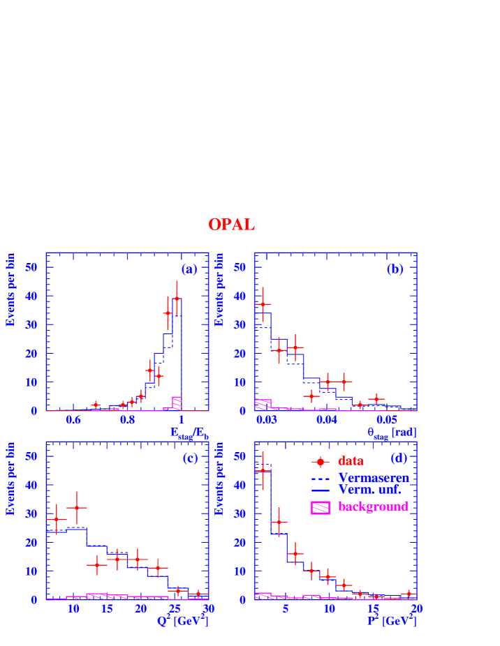
Figure 4: Comparison of the data with the Monte Carlo predictions for the DB samples. Figures (a,b) and (c,d) are for the DB1 and DB2 samples, respectively. Shown are (a) the energy of the second detected electron normalised to the energy of the beam electrons, $E_{\rm stag}$/$E_{\rm b}$, (b) the polar angle of the second detected electron, $\theta_{\rm stag}$, (c) the measured $Q^{2}$, and (d) the measured $P^{2}$. The points represent the data with the statistical error only. The dashed lines denote the distributions of the Vermaseren Monte Carlo with the background added to it before the unfolding is performed, the full lines are the same distributions after reweighting based on the unfolding procedure, and the hatched histograms represent the background contribution

Figure 15: The measured structure functions $F_{\mathrm{A}}^{\gamma}$ and $F_{\mathrm{B}}^{\gamma}$ for the combined SW and FD sample. The points represent the data with their statistical (inner error bars) and total errors (outer error bars). The solid lines are the QED predictions for $Q^{2}=5.4$ $\rm GeV^{2}$ and $\epsilon=\rho=1$. $\chi^{2}/{\rm dof}=3.5/4$ for $F_{\mathrm{A}}^{\gamma}$ and $\chi^{2}/{\rm dof}=3.8/4$ for $F_{\mathrm{B}}^{\gamma}$

References

- [1] V.M. Budnev, I.F. Ginzburg, G.V. Meledin, and V.G. Serbo, Phys. Rep. 15, 181 (1975).
- [2] C. Peterson, P.M. Zerwas, and T.F. Walsh, Nucl. Phys. B229, 301 (1983).
-
[3]
CELLO Collaboration,
H.J. Behrend et al.,
Phys. Lett. 126B, 384 (1983);
TPC/2 Collaboration, M.P. Cain et al., Phys. Lett. 147B, 232 (1984);
PLUTO Collaboration, C. Berger et al., Z. Phys. C27, 249 (1985). - [4] OPAL Collaboration, R. Akers et al., Z. Phys. C60, 593 (1993).
- [5] DELPHI Collaboration, P. Abreu et al., Z. Phys. C69, 223 (1996).
-
[6]
L3 Collaboration,
M. Acciarri et al.,
Phys. Lett. B438, 363 (1998).
- [7] OPAL Collaboration, K. Ackerstaff et al., Z. Phys. C74, 49 (1997).
- [8] C. Berger and W. Wagner, Phys. Rep. 146, 1 (1987).
- [9] P. Kessler, Il Nuovo Cimento 17, 809 (1960).
-
[10]
C.F. von Weizsäcker,
Z. Phys. 88, 612 (1934);
E.J. Williams, Phys. Rev. 45, 729 (1934). - [11] PLUTO Collaboration, C. Berger et al., Phys. Lett. 142B, 119 (1984).
- [12] N. Arteaga, C. Carimalo, P. Kessler, and S. Ong, Phys. Rev. D52, 4920 (1995).
- [13] R. Nisius, M.H. Seymour, RAL-TR-1998-079, (1998), hep-ph/9812281, to be published in Phys. Lett. B.
- [14] P. Aurenche, G. Schuler, et al., physics, in Proceedings of Physics at LEP2 Vol1., edited by G. Altarelli, T. Sjöstrand, and F. Zwirner, p291, 1996, CERN 96-01.
-
[15]
J. Smith, J.A.M. Vermaseren, and G. Grammer Jr.,
Phys. Rev. D15, 3280 (1977);
J.A.M. Vermaseren, J. Smith, and G. Grammer Jr., Phys. Rev. D19, 137 (1979);
J.A.M. Vermaseren, Nucl. Phys. B229, 347 (1983). - [16] R. Bhattacharya, G. Grammer Jr., and J. Smith, Phys. Rev. D15, 3267 (1977).
-
[17]
F. Berends, P. Daverveldt, and R. Kleiss,
Nucl. Phys. B253, 421 (1985);
F. Berends, P. Daverveldt, and R. Kleiss, Comp. Phys. Comm. 40, 271 (1986);
F. Berends, P. Daverveldt, and R. Kleiss, Comp. Phys. Comm. 40, 285 (1986);
F. Berends, P. Daverveldt, and R. Kleiss, Nucl. Phys. B264, 243 (1986). - [18] G.A. Schuler, Comp. Phys. Comm. 108, 279 (1998).
- [19] J. Hilgart, R. Kleiss, and F.L. Diberder, Comp. Phys. Comm. 75, 191 (1993).
- [20] J. Fujimoto et al., Comp. Phys. Comm. 100, 128 (1997).
-
[21]
OPAL Collaboration,
K. Ahmet et al.,
Nucl. Instr. and Meth. A305, 275 (1991);
P.P. Allport et al., Nucl. Instr. and Meth. A324, 34 (1993);
P.P. Allport et al., Nucl. Instr. and Meth. A346, 476 (1994);
B.E. Anderson et al., IEEE Transactions on Nuclear Science 41, 845 (1994). -
[22]
G. Marchesini and B.R. Webber,
Nucl. Phys. B310, 461 (1988);
I.G. Knowles, Nucl. Phys. B310, 571 (1988);
S. Catani, G. Marchesini, and B.R. Webber, Nucl. Phys. B349, 635 (1991);
G. Abbiendi and L. Stanco, Comp. Phys. Comm. 66, 16 (1991);
M.H. Seymour, Z. Phys. C56, 161 (1992). - [23] S. Jadach, B.F.L. Ward, and Z. Wa̧s, Comp. Phys. Comm. C79, 503 (1994).
- [24] J. Allison et al., Nucl. Instr. and Meth. A317, 47 (1992).
-
[25]
V. Blobel,
DESY84-118 (1984);
V. Blobel, Regularized Unfolding for High-Energy Physics Experiments, RUN program manual, unpublished (1996). -
[26]
OPAL Collaboration,
K. Ackerstaff et al.,
Z. Phys. C74, 33 (1997);
OPAL Collaboration, K. Ackerstaff et al., Phys. Lett. B411, 387 (1997);
OPAL Collaboration, K. Ackerstaff et al., Phys. Lett. B412, 225 (1997). - [27] A. Buijs, W.G.J. Langeveld, M.H. Lehto, and D.J. Miller, Comp. Phys. Comm. 79, 523 (1994).