Hadronic Structure in the Decay $\tau^{-}\rightarrow\nu_{\tau}\pi^{-}\pi^{0}\pi^{0}$
and the Sign of the Tau Neutrino Helicity

Abstract

Based on a sample corresponding to $4.3\times 10^{6}$ produced $\tau$-pair events, we have studied hadronic dynamics in the decay $\tau^{-}\to\nu_{\tau}\pi^{-}\pi^{0}\pi^{0}$ in data recorded by the CLEO II detector operating at the CESR $e^{+}e^{-}$ collider. The decay is dominated by the process $\tau^{-}\to\nu_{\tau}a_{1}^{-}(1260)$, with the $a_{1}^{-}$ meson decaying to three pions predominantly via the lowest dimensional (mainly $S$-wave) $a_{1}\to\rho^{-}\pi^{0}$ Born amplitude. From model-dependent fits to the Dalitz plot and angular observables in bins of $3\pi$ mass, we find significant additional contributions from amplitudes for $a_{1}$ decay to $\sigma\pi$, $f_{0}(1370)\pi$ and $f_{2}(1270)\pi$, as well as higher dimensional $a_{1}\to\rho\pi$ and $\rho^{\prime}\pi$ amplitudes. Notably, the squared $\sigma\pi$ amplitude accounts for approximately 15$\%$ of the total $\tau^{-}\to\nu_{\tau}\pi^{-}\pi^{0}\pi^{0}$ rate in the models considered. The data are well described using couplings to these amplitudes that are independent of the $3\pi$ mass. These amplitudes also provide a good description for the $\tau^{-}\to\nu_{\tau}\pi^{-}\pi^{+}\pi^{-}$ Dalitz plot distributions. We have searched for additional contributions from $\tau^{-}\to\nu_{\tau}\pi^{\prime-}(1300)$. We place $90\%$ confidence level upper limits on the branching fraction for this channel of between $1.0\times 10^{-4}$ and $1.9\times 10^{-4}$, depending on the $\pi^{\prime}$ decay mode considered. The $\pi^{-}\pi^{0}\pi^{0}$ mass spectrum is parametrized by a Breit-Wigner form with a mass-dependent width which is specified according to the results of the Dalitz plot fits plus an unknown coupling to an $a_{1}\to K^{*}K$ amplitude. From a $\chi^{2}$ fit using this parametrization, we extract the pole mass and width of the $a_{1}$, as well as the magnitude of the $K^{*}K$ coupling. We have also investigated the impact of a possible contribution from the $a_{1}^{\prime}(1700)$ meson on this spectrum. Finally, exploiting the parity-violating angular asymmetry in $a_{1}\to 3\pi$ decay, we determine the signed value of the $\tau$ neutrino helicity to be $h_{\nu_{\tau}}=-1.02\pm 0.13\,\mbox{(stat.)}\pm 0.03\,\mbox{(syst.$+$model)}$, confirming the left-handedness of the $\tau$ neutrino.

D. M. Asner,¹ A. Eppich,¹ J. Gronberg,¹ T. S. Hill,¹ D. J. Lange,¹ R. J. Morrison,¹ H. N. Nelson,¹ T. K. Nelson,¹ D. Roberts,¹ B. H. Behrens,² W. T. Ford,² A. Gritsan,² H. Krieg,² J. Roy,² J. G. Smith,² J. P. Alexander,³ R. Baker,³ C. Bebek,³ B. E. Berger,³ K. Berkelman,³ V. Boisvert,³ D. G. Cassel,³ D. S. Crowcroft,³ M. Dickson,³ S. von Dombrowski,³ P. S. Drell,³ K. M. Ecklund,³ R. Ehrlich,³ A. D. Foland,³ P. Gaidarev,³ R. S. Galik,³ L. Gibbons,³ B. Gittelman,³ S. W. Gray,³ D. L. Hartill,³ B. K. Heltsley,³ P. I. Hopman,³ D. L. Kreinick,³ T. Lee,³ Y. Liu,³ T. 0. Meyer,³ N. B. Mistry,³ C. R. Ng,³ E. Nordberg,³ M. Ogg,^3, J. R. Patterson,³ D. Peterson,³ D. Riley,³ A. Soffer,³ J. G. Thayer,³ P. G. Thies,³ B. Valant-Spaight,³ A. Warburton,³ C. Ward,³ M. Athanas,⁴ P. Avery,⁴ C. D. Jones,⁴ M. Lohner,⁴ C. Prescott,⁴ A. I. Rubiera,⁴ J. Yelton,⁴ J. Zheng,⁴ G. Brandenburg,⁵ R. A. Briere,⁵ A. Ershov,⁵ Y. S. Gao,⁵ D. Y.-J. Kim,⁵ R. Wilson,⁵ T. E. Browder,⁶ Y. Li,⁶ J. L. Rodriguez,⁶ H. Yamamoto,⁶ T. Bergfeld,⁷ B. I. Eisenstein,⁷ J. Ernst,⁷ G. E. Gladding,⁷ G. D. Gollin,⁷ R. M. Hans,⁷ E. Johnson,⁷ I. Karliner,⁷ M. A. Marsh,⁷ M. Palmer,⁷ C. Plager,⁷ C. Sedlack,⁷ M. Selen,⁷ J. J. Thaler,⁷ J. Williams,⁷ K. W. Edwards,⁸ A. Bellerive,⁹ R. Janicek,⁹ P. M. Patel,⁹ A. J. Sadoff,¹⁰ R. Ammar,¹¹ P. Baringer,¹¹ A. Bean,¹¹ D. Besson,¹¹ D. Coppage,¹¹ R. Davis,¹¹ S. Kotov,¹¹ I. Kravchenko,¹¹ N. Kwak,¹¹ X. Zhao,¹¹ L. Zhou,¹¹ S. Anderson,¹² Y. Kubota,¹² S. J. Lee,¹² R. Mahapatra,¹² J. J. O’Neill,¹² R. Poling,¹² T. Riehle,¹² A. Smith,¹² M. S. Alam,¹³ S. B. Athar,¹³ Z. Ling,¹³ A. H. Mahmood,¹³ S. Timm,¹³ F. Wappler,¹³ A. Anastassov,¹⁴ J. E. Duboscq,¹⁴ K. K. Gan,¹⁴ C. Gwon,¹⁴ T. Hart,¹⁴ K. Honscheid,¹⁴ H. Kagan,¹⁴ R. Kass,¹⁴ J. Lorenc,¹⁴ H. Schwarthoff,¹⁴ A. Wolf,¹⁴ M. M. Zoeller,¹⁴ S. J. Richichi,¹⁵ H. Severini,¹⁵ P. Skubic,¹⁵ A. Undrus,¹⁵ M. Bishai,¹⁶ S. Chen,¹⁶ J. Fast,¹⁶ J. W. Hinson,¹⁶ J. Lee,¹⁶ N. Menon,¹⁶ D. H. Miller,¹⁶ E. I. Shibata,¹⁶ I. P. J. Shipsey,¹⁶ S. Glenn,¹⁷ Y. Kwon,^17, A.L. Lyon,¹⁷ E. H. Thorndike,¹⁷ C. P. Jessop,¹⁸ K. Lingel,¹⁸ H. Marsiske,¹⁸ M. L. Perl,¹⁸ V. Savinov,¹⁸ D. Ugolini,¹⁸ X. Zhou,¹⁸ T. E. Coan,¹⁹ V. Fadeyev,¹⁹ I. Korolkov,¹⁹ Y. Maravin,¹⁹ I. Narsky,¹⁹ R. Stroynowski,¹⁹ J. Ye,¹⁹ T. Wlodek,¹⁹ M. Artuso,²⁰ S. Ayad,²⁰ E. Dambasuren,²⁰ S. Kopp,²⁰ G. Majumder,²⁰ G. C. Moneti,²⁰ R. Mountain,²⁰ S. Schuh,²⁰ T. Skwarnicki,²⁰ S. Stone,²⁰ A. Titov,²⁰ G. Viehhauser,²⁰ J.C. Wang,²⁰ S. E. Csorna,²¹ K. W. McLean,²¹ S. Marka,²¹ Z. Xu,²¹ R. Godang,²² K. Kinoshita,^22, I. C. Lai,²² P. Pomianowski,²² S. Schrenk,²² G. Bonvicini,²³ D. Cinabro,²³ R. Greene,²³ L. P. Perera,²³ G. J. Zhou,²³ S. Chan,²⁴ G. Eigen,²⁴ E. Lipeles,²⁴ M. Schmidtler,²⁴ A. Shapiro,²⁴ W. M. Sun,²⁴ J. Urheim,²⁴ A. J. Weinstein,²⁴ F. Würthwein,²⁴ D. E. Jaffe,²⁵ G. Masek,²⁵ H. P. Paar,²⁵ E. M. Potter,²⁵ S. Prell,²⁵ and V. Sharma²⁵

I INTRODUCTION

The decay  $\tau^{-}\to\nu_{\tau}[3\pi]^{-}$ has been the subject of much interest over the years. Because of the transformation properties of the weak current under parity and G-parity, $\tau$ lepton decay to an odd number of pions is expected to occur exclusively through the axial vector current, ignoring isospin-violating effects. Thus the $3\pi$ system in this decay must have spin-parity quantum numbers $J^{P}=0^{-}$ or $1^{+}$. As a result of this plus the purely weak interaction involved in $\tau$ decay, such decays provide an excellent opportunity to investigate the axial vector hadronic weak current and the dynamics of axial vector meson decay.

The $\tau^{-}\to\nu_{\tau}[3\pi]^{-}$ decay is dominated by production of the poorly understood $a_{1}(1260)$ meson, which is believed to decay mainly via the lowest dimensional Born (mostly $S$-wave) $\rho\pi$ intermediate state. The world average values [1] for its mass and width are $1230\pm 40$ and 250–600 MeV respectively, determined primarily from $\tau$ decay. The theoretical understanding of the $a_{1}$ is not rigorous – many models have been proposed [2, 3, 4, 5, 6, 7] to describe the line shape and resonant substructure, but none have provided an entirely satisfactory description of the data. Additional experimental input is essential for a better understanding of this system.

Recent experimental studies of the $\tau^{-}\to\nu_{\tau}\pi^{-}\pi^{+}\pi^{-}$ decay have been carried out by the ARGUS [8, 9], OPAL [10] and DELPHI [11, 12] collaborations. Analyses of earlier data such as that by Isgur, Morningstar and Reader [4] had demonstrated the presence of $D$-wave $\rho\pi$ production. With $\sim 7,500$ events, ARGUS [8] measured the ratio of amplitudes at the nominal $a_{1}$ mass to be $D/S=-0.11\pm 0.02$. In a sample of $\sim 6,300$ events, OPAL [10] found $D/S=-0.10\pm 0.02\pm 0.02$. Another ARGUS analysis [9] of $\sim 3,300$ lepton-tagged events considered many additional amplitudes. This analysis found a signal at the $4.2$ standard deviation ($\sigma$) level for the presence of an $a_{1}\to f_{2}(1270)\pi$ amplitude. Neither ARGUS nor OPAL found evidence of non-axial-vector contributions such as production of the $J^{P}=0^{-}$ $\pi^{\prime}(1300)$ which decays via $\rho\pi$ and $\sigma\pi$.

In addition, the decays $\tau^{-}\to\nu_{\tau}[3\pi]^{-}$ and $\tau^{-}\to\nu_{\tau}[5\pi]^{-}$ have been employed to constrain the $\tau$ neutrino mass [11, 13], through investigation of the endpoint in the invariant mass and energy spectra of the multi-pion system. Notably, ALEPH [14] has obtained an upper limit of 18.2 MeV at the 95$\%$ confidence level (CL) on the $\nu_{\tau}$ mass, based on these decays. These analyses rely on an understanding of the hadronic dynamics. DELPHI [11, 12], with $\sim 6,500$ events, has reported anomalous structure in $\tau^{-}\to\nu_{\tau}\pi^{-}\pi^{+}\pi^{-}$ in the context of a $\nu_{\tau}$ mass analysis. In that work, the Dalitz plot distribution for events with very high $3\pi$ mass ($>1.5\,\mbox{GeV}$) is suggestive of enhanced $D$-wave $\rho\pi$ production, while the $3\pi$ mass spectrum shows an excess in this region relative to expectations from a single $a_{1}$ resonance. Inclusion of a radial excitation (an $a_{1}^{\prime}$) with a large $D$-wave coupling to $\rho\pi$ provides an improved description of the DELPHI data, but weakens the $\nu_{\tau}$ mass limit.

In this article, we present results from a model-dependent analysis of the decay $\tau^{-}\to\nu_{\tau}\pi^{-}\pi^{0}\pi^{0}$, based on data collected with the CLEO II detector. We perform fits to models to characterize both the substructure as seen in Dalitz plot and angular variables, as well as the $a_{1}$ resonance parameters as seen in the $3\pi$ invariant mass spectrum. The $\pi^{-}\pi^{0}\pi^{0}$ channel has several advantages relative to the all-charged mode. First, the multihadronic and $\tau$ feed-across backgrounds are smaller. Second, the $\pi^{-}\pi^{0}\pi^{0}$ mode may be better suited for discerning substructure involving isoscalar mesons because there is only one pairing of pions which can have $I=0$, unlike in the all-charged case. This second point is particularly relevant in light of the ARGUS result for $f_{2}\pi$ production [9] and the recent observation of the decay $\tau^{-}\to\nu_{\tau}f_{1}(1285)\pi^{-}$ by CLEO [15]. These results suggest that isoscalars may play a role in $a_{1}$ decay.

The outline for the article is as follows. In Section II, we describe the data sample and event selection. We describe the basic elements of the model used to characterize the $\tau^{-}\to\nu_{\tau}\pi^{-}\pi^{0}\pi^{0}$ data in Section III. In Sections IV, V and VI, we describe the three analyses of the hadronic structure: (1) performing fits to the substructure based on Dalitz plot and angular observables; (2) extending these fits to determine the signed $\tau$ neutrino helicity; and (3) performing fits to determine the resonant structure of the $3\pi$ mass spectrum, making use of results from the substructure fits. We summarize the results and conclude in Section VII.

II DATA SAMPLE AND EVENT SELECTION

The analysis described here is based on 4.67 fb^-1 of $e^{+}e^{-}$ collision data collected at center-of-mass energies $2E_{\rm beam}$ of $\sim 10.6$ GeV, corresponding to $4.3\times 10^{6}$ reactions of the type $e^{+}e^{-}\to\tau^{+}\tau^{-}$. These data were recorded at the Cornell Electron Storage Ring (CESR) with the CLEO II detector [16] between 1990 and 1995. Charged particle tracking in CLEO II consists of a cylindrical six-layer straw tube array surrounding a beam pipe of radius 3.2 cm that encloses the $e^{+}e^{-}$ interaction point (IP), followed by two co-axial cylindrical drift chambers of 10 and 51 sense wire layers respectively. Barrel ($|\cos\theta|<0.81$, where $\theta$ is the polar angle relative to the beam axis) and end cap scintillation counters used for triggering and time-of-flight measurements surround the tracking chambers. For electromagnetic calorimetry, 7800 CsI(Tl) crystals are arrayed in projective (toward the IP) and axial geometries in barrel and end cap sections respectively. The barrel crystals present 16 radiation lengths to photons originating from the IP.

Identification of $\tau^{-}\to\nu_{\tau}\pi^{-}\pi^{0}\pi^{0}$ decays relies heavily on the segmentation and energy resolution of the calorimeter for reconstruction of the $\pi^{0}$’s. The central portion of the barrel calorimeter ($|\cos\theta|<0.71$) achieves energy and angular resolutions of $\sigma_{E}/E\,(\%)=0.35\,E^{0.75}+1.9-0.1\,E$ and $\sigma_{\phi}\,\mbox{(mrad)}=2.8/\sqrt{E}+2.5$, with $E$ in GeV, for electromagnetic showers. The angular resolution ensures that the two clusters of energy deposited by the photons from a $\pi^{0}$ decay are resolved over the range of $\pi^{0}$ energies typical of the $\tau$ decay mode studied here.

The detector elements described above are immersed in a 1.5 Tesla magnetic field provided by a superconducting solenoid surrounding the calorimeter. Muon identification is accomplished with proportional tubes embedded in the flux return steel at depths representing 3, 5 and 7 interaction lengths of total material penetration at normal incidence.

A Event selection

To identify events as $\tau\tau$ candidates we require the decay of the $\tau^{+}$ (denoted as the ‘tagging’ decay) that is recoiling against our signal $\tau^{-}$ decay to be classified as $\overline{\nu}_{\tau}e^{+}\nu_{e}$, $\overline{\nu}_{\tau}\mu^{+}\nu_{\mu}$, $\overline{\nu}_{\tau}\pi^{+}$, or $\overline{\nu}_{\tau}\pi^{+}\pi^{0}$. Thus, we select events containing two oppositely charged barrel tracks separated in angle by at least $90^{\circ}$. To reject backgrounds from Bhabha scattering and two-photon interactions we require track momenta to be between $0.08\,E_{\rm beam}$ and $0.90\,E_{\rm beam}$. Clusters of energy deposition in the central region of the calorimeter ($|\cos\theta|<0.71$) that are not matched with a charged track projection are paired to form $\pi^{0}$ candidates. These showers must have energies greater than 50 MeV, and the invariant mass of the photon-pair must lie within $7.5\sigma$ of the $\pi^{0}$ mass where $\sigma$ varies between $\sim 4-7$ MeV. Those $\pi^{0}$ candidates with energy above $0.06\,E_{\rm beam}$ after application of a $\pi^{0}$ mass constraint are associated with any track within $90^{\circ}$.

A $\pi^{-}\pi^{0}\pi^{0}$ candidate is formed from a track which has two associated $\pi^{0}$ candidates as defined above. If more than one combination of $\pi^{0}$ candidates can be assigned to a given track, only one combination is chosen: namely, that for which the largest unused barrel photon-like cluster in the $\pi^{-}\pi^{0}\pi^{0}$ hemisphere has the least energy. A cluster is defined to be photon-like if it satisfies a $1\%$ confidence level cut on the transverse shower profile and lies at least 30 cm away from the nearest track projection.

As mentioned earlier, to reject background from multihadronic ($e^{+}e^{-}\to q\overline{q}$) events, the tag system recoiling against the $\pi^{-}\pi^{0}\pi^{0}$ candidate must be consistent with $\tau$ decay to neutrino(s) plus $e^{+}$, $\mu^{+}$, $\pi^{+}$ or $\pi^{+}\pi^{0}$ (denoted as $\rho^{+}$). The recoiling track is identified as an electron if its calorimeter energy to track momentum ratio satisfies $0.85<E/p<1.1$ and if its specific ionization in the main drift chamber is not less than $2\sigma$ below the value expected for electrons. It is classified as a muon if the track has penetrated to at least the innermost layer of muon chambers at 3 interaction lengths. If not identified as an $e$ or a $\mu$, then if the track is accompanied by a third $\pi^{0}$ of energy $\geq 350\,{\mbox{M}eV}$ which lies closer to it than to the $\pi 2\pi^{0}$ system, the track-$\pi^{0}$ combination is classified as a $\rho$ tag. The invariant mass of this system must be between 0.55 and 1.20 GeV. If not identified as an $e$, $\mu$, or $\rho$ tag, the recoil track is identified as a single $\pi$ tag. To ensure that these classifications are consistent with expectations from $\tau$ decay, events are vetoed if any unused photon-like cluster with $|\cos\theta|<0.95$ has energy greater than 200 MeV, or if any unmatched non-photon-like cluster has energy above 500 MeV. The missing momentum as determined using the $\pi 2\pi^{0}$ and tagging systems must point into a high-acceptance region of the detector ($|\cos\theta_{\rm miss}|<0.9$), and must have a component transverse to the beam of at least $0.06\,E_{\rm beam}$.

B Final event sample

After all cuts, the remaining sample consists of 51,136 events. The normalized invariant masses of the two photon-pairs, $S_{\gamma\gamma}\equiv(M_{\gamma\gamma}-m_{\pi^{0}})/\sigma_{\gamma\gamma}$, are plotted against each other in Fig. 1(a). In Fig. 1(b), $S_{\gamma\gamma}$ is plotted for all $\pi^{0}$ candidates along with the corresponding distribution from the $\tau$ Monte Carlo (MC) sample described in the following section.

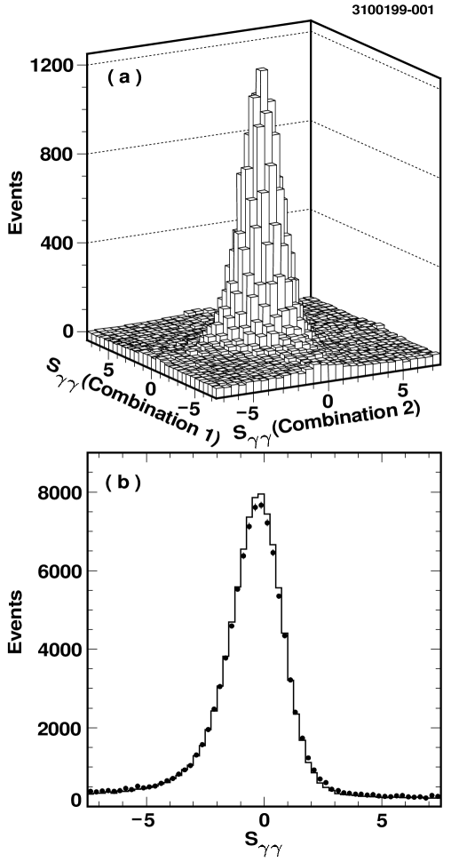
FIG. 1.: (a) Plot of the normalized photon-pair invariant mass $S_{\gamma\gamma}=(M_{\gamma\gamma}-m_{\pi^{0}})/\sigma_{\gamma\gamma}$ for the two $\pi^{0}$ candidates after all other cuts have been applied. (b) Comparison of the $S_{\gamma\gamma}$ distribution (two entries per event) for data (points) and $\tau\tau$ Monte Carlo (histogram) samples.

We define the $\pi^{0}\pi^{0}$ signal region to be that where $-3.0<S_{\gamma\gamma}<2.0$ for both $\pi^{0}$ candidates. In the $\pi^{0}\pi^{0}$ signal region there are 36710 events, of which 17234 are tagged by leptonic decays of the recoiling $\tau$. To estimate the contributions from fake $\pi^{0}$’s, we also define side and corner band regions using $-7.5<S_{\gamma\gamma}<-5.0$ and $3.0<S_{\gamma\gamma}<5.5$.

In Fig. 2, we plot the $\pi^{-}\pi^{0}\pi^{0}$ mass for events in the $\pi^{0}\pi^{0}$ signal and side band regions, for data and $\tau$ MC samples.

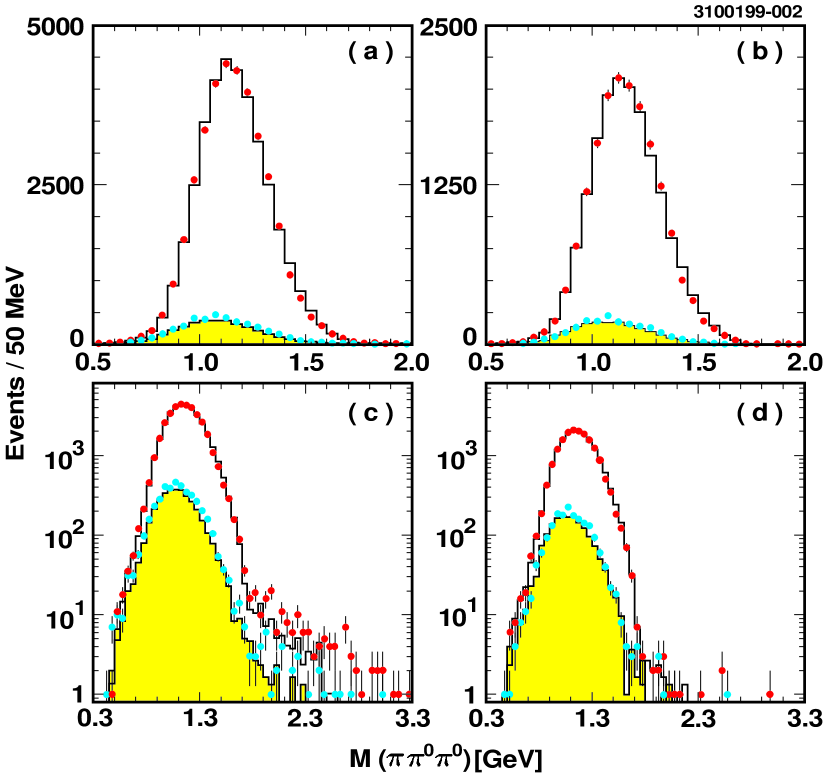
FIG. 2.: $\pi^{-}\pi^{0}\pi^{0}$ mass spectrum from the all-tag (a) and lepton tag (b) samples, after cuts. Shown are events in the $\pi^{0}\pi^{0}$ signal (dark points for the data, unshaded histogram for the Monte Carlo spectrum) and side band (light points for the data, shaded histogram for the MC spectrum) regions. Plots (c) and (d) show the same spectra as in (a) and (b) plotted over a larger range and on a logarithmic scale.

The events above the $\tau$ mass in Fig. 2(c) are dominantly due to feedacross from $\tau\to\rho\nu$ decays where the second $\pi^{0}$ is being picked up from the recoil $\tau$ decay. The $\tau$ Monte Carlo simulation accounts for most of this high mass tail, but not all, with the remainder being due to a small $q\overline{q}$ background contribution. The high mass events are essentially absent from the lepton-tagged events, plotted in Fig. 2(d).

C Monte Carlo samples

For determination of detection efficiency for our signal decay as well as for backgrounds from other $\tau$ decay modes, we rely on a sample of Monte Carlo $e^{+}e^{-}\to\tau^{+}\tau^{-}$ events with equivalent luminosity approximately three times that of the data. These events were generated using the KORALB/TAUOLA [17] program, and then passed through the GEANT-based [18] CLEO II detector simulation package. The full CLEO event reconstruction program was then run on this sample. The MC distributions shown in Figs. 1 and 2 are derived from this sample.

In TAUOLA, the $\tau^{-}\to\nu_{\tau}[3\pi]^{-}$ decay is described with a single $a_{1}$ resonance decaying solely via the lowest dimensional ($s$-wave, in the notation introduced in the next section) Born amplitude for $(\rho+\rho^{\prime})\,\pi$ production, following the model of Kühn and Santamaria [5]. We have tuned the $a_{1}$ mass and width to yield a $3\pi$ mass spectrum that roughly matches that seen in our data in the all-charged mode. Although the data and MC $3\pi$ mass spectra show reasonable agreement on average (see Fig. 2), close inspection reveals significant deviations, particularly in the high mass region located roughly between 1.4 GeV and the $\tau$ mass. The Dalitz plot distributions agree poorly with the corresponding MC distributions, especially in the $M_{\pi^{0}\pi^{0}}$ projection and most strikingly at high $3\pi$ mass.

For the substructure fits described in Section IV, we generated additional MC samples for our signal mode plus key background $\tau$ decay modes. For these samples, we developed special purpose event generators. Unlike the treatment in KORALB/TAUOLA, we implemented radiative effects according to an approximation in which they factorize from the rest of the differential matrix element, as required by the reverse Monte Carlo approach described in Section IV A. In addition, the signal mode was generated with a $3\pi$ mass spectrum weighted towards high values so as to ensure high statistics in the high-mass region where the data show the most apparent deviation from the model used by TAUOLA in both Dalitz plot and $3\pi$ mass distributions.

III MODEL OF $\tau^{-}\to\nu_{\tau}\pi^{-}\pi^{0}\pi^{0}$

Tau lepton decay to neutrino plus three pions follows the form

$$d\Gamma(\tau\to\nu_{\tau}3\pi)=\frac{1}{2m_{\tau}}\left[\frac{G_{F}^{2}V_{ud}}{2}L^{\mu\nu}J_{\mu}J^{*}_{\nu}\right]d\Phi_{4},$$ (1)

where $L^{\mu\nu}$ represents the lepton tensor for weak decay, $J^{\mu}$ denotes the hadronic weak current for production of three pions, and $d\Phi_{4}$ is the Lorentz-invariant 4-body phase space element for the decay. The goal of this analysis is to probe the structure of the hadronic current, benefitting from the well-understood properties of the weak interaction.

In principle $J^{\mu}$ is comprised of vector and axial vector currents:

$$J^{\mu}=J_{V}^{\mu}+J_{A}^{\mu}=<3\pi|\overline{d}\gamma_{\mu}u|0>+<3\pi|\overline{d}\gamma_{5}\gamma_{\mu}u|0>,$$ (2)

however $G$-parity conservation requires that $J^{V}_{\mu}=0$. Thus we consider only contributions from the axial vector current.

In $\tau$ decay, the squared momentum transfer $s\equiv M_{3\pi}^{2}$ is small, and thus the dynamics are expected to be dominated by resonance production. The possible axial vector ($J^{P}=1^{+}$) resonance contributions are the $a_{1}(1260)$ and radial excitations, i.e., the $a_{1}^{\prime}$. In addition, pseudoscalar ($J^{P}=0^{-}$) contributions are possible, i.e., the $\pi^{\prime}(1300)$, although these are expected to be suppressed according to the Partially Conserved Axial Current (PCAC) hypothesis. In this section we describe the model used to parametrize $J^{\mu}$, assuming the $3\pi$ system is in a $J^{P}=1^{+}$ state.

A Model for substructure in $1^{+}\to 3\pi$

The strong decay of the $a_{1}$ is expected to involve substructure which is again dominated by resonance production. We write for the contribution to $J^{\mu}$ involving $a_{1}$ production

$$J^{\mu}_{a_{1}}=B_{a_{1}}(s)\times\sum_{i}\beta_{i}\,j^{\mu}_{i},$$ (3)

where $B_{a_{1}}(s)$ denotes the $a_{1}$ Breit-Wigner, $\beta_{i}$ are complex coupling constants, and $j^{\mu}_{i}$ contain form factors describing components of the substructure involving specific resonances. The details of this parametrization are given in Appendix A. As an example, in the case of $s$-wave $\rho\pi$ production,

$$j^{\mu}_{\rho\pi,\,s\mbox{-wave}}=T^{\mu\nu}\left[q_{1\nu}\,B_{\rho}(s_{1})\,F_{R_{\rho\pi}}(k_{1})-q_{2\nu}\,B_{\rho}(s_{2})\,F_{R_{\rho\pi}}(k_{2})\right].$$ (4)

We define $p_{1}$, $p_{2}$ and $p_{3}$ as the four-momenta of the three pions, in our case $\pi^{0}_{1}$, $\pi^{0}_{2}$ and $\pi^{-}$, respectively. We define $a=p_{1}+p_{2}+p_{3}$, $s_{i}=(p_{j}+p_{k})^{2}$ and $q_{i}=p_{j}-p_{k}$, where $(i,j,k)$ represent cyclic permutations of $(1,2,3)$. The factor $T^{\mu\nu}$ denotes the expression $g^{\mu\nu}-a^{\mu}a^{\nu}/a^{2}$. The factors $B_{\rho}(s_{i})$ denote Breit-Wigners describing the corresponding $\rho\to\pi\pi^{0}$ amplitudes. Finally, we have included an additional form factor $F_{R_{\rho\pi}}$, which represents the effect of the finite size of the $a_{1}$ meson in its decay to $\rho\pi$. We take this form factor to have the form

$$F_{R_{i}}(k_{i})=e^{-R_{i}^{2}k_{i}^{2}/2},$$ (5)

where $k_{i}$ is the momentum of the decay products, the $\rho$ and the $\pi$ in this case, in the $a_{1}$ rest frame. The parameter $R_{i}$ is proportional (by a factor of $\sqrt{6}\hbar c$, see Ref. [3]) to the root mean square (r.m.s.) radius of the $a_{1}$. We note that expressions for $j^{\mu}_{i}$ must be symmetric with respect to interchange of $\pi^{0}_{1}$ and $\pi^{0}_{2}$ since these are indistinguishable.

In our analysis of substructure in the $\tau\to\nu_{\tau}3\pi$ decay, we consider the following amplitudes:

$$\begin{array}[]{cl}j_{1}^{\mu}:&\mbox{$s$-wave amplitude for $1^{+}\rightarrow\rho(770)\pi$ (denoted as $\rho\pi$)},\\ j_{2}^{\mu}:&\mbox{$s$-wave amplitude for $1^{+}\rightarrow\rho(1450)\pi$ (denoted as $\rho^{\prime}\pi$)},\\ j_{3}^{\mu}:&\mbox{$d$-wave amplitude for $1^{+}\rightarrow\rho(770)\pi$},\\ j_{4}^{\mu}:&\mbox{$d$-wave amplitude for $1^{+}\rightarrow\rho(1450)\pi$},\\ j_{5}^{\mu}:&\mbox{$p$-wave amplitude for $1^{+}\rightarrow f_{2}(1270)\pi$},\\ j_{6}^{\mu}:&\mbox{$p$-wave amplitude for $1^{+}\rightarrow f_{0}(400-1200)\pi$ (denoted as $\sigma\pi$)},\\ j_{7}^{\mu}:&\mbox{$p$-wave amplitude for $1^{+}\rightarrow f_{0}(1370)\pi$}.\end{array}$$ (6)

An explicit parametrization of the amplitudes $j_{i}^{\mu}$ is given by Eqn. A5. With these definitions, the constants $\beta_{i}$ have dimensions of [GeV]^x, where the exponent depends on the amplitude. In our fits we specify $\beta_{1}=1$, such that the couplings for the other amplitudes are determined relative to the $s$-wave $\rho\pi$ coupling. The parameters used to describe the resonances appearing in the $j^{\mu}_{i}$ above are given in Table I, while the Breit-Wigner form used here is given in Appendix A by Eqn. A11.

TABLE I.: Resonance parameters for the intermediate states as used in the substructure fits.

$Y$	$m_{0Y}$	$\Gamma_{0}^{Y}$	Ref.
	[GeV]	[GeV]
$\rho(770)$	$0.774$	$0.149$	[19]
$\rho(1450)$	$1.370$	$0.386$	[19]
$f_{2}(1270)$	$1.275$	$0.185$	[1]
$\sigma$	$0.860$	$0.880$	[20]
$f_{0}(1370)$	$1.186$	$0.350$	[20]

In Eqns. 4 and A5, we have constructed Lorentz-invariant amplitudes so as to make contact with the resonant components of the substructure. In contrast with a formulation based on angular momentum eigen functions, these amplitudes are only approximately associated with a specific angular momentum quantum number $L$, and hence we have employed lower case letters to identify the primary value of $L$. Thus, for example the lowest dimensional Born amplitude for $\rho\pi$, the Lorentz-invariant $s$-wave amplitude, contains a small $D$-wave component (see for example, Refs. [4, 6]).

The selection of the amplitudes $j^{\mu}_{1},\ldots,j^{\mu}_{7}$ is in part based on experience gained in early attempts to fit the data. It is also in part motivated by the unitarized quark model of Törnqvist [20]. The resonance parameters of the broader $\sigma$ and $f_{0}(1370)$ mesons are taken from application of this model to existing data [20]. We have also performed fits with additional amplitudes, namely the axial vector $f_{0}(980)\pi$ and pseudoscalar $\pi^{\prime}\to\rho\pi$ and $\sigma\pi$. These are discussed in Section IV D.

B Model for the $3\pi$ mass spectrum

The conventional understanding of $\tau\to\nu_{\tau}\,3\pi$ decay is that it proceeds through creation of the lowest lying axial vector meson, the $a_{1}(1260)$. Since radial excitations may also be present, we replace the Breit-Wigner function $B_{a_{1}}(s)$ appearing in Eqn. 3 by a modified function that includes a possible $a_{1}^{\prime}$ admixture.

$$B(s)=B_{a_{1}}(s)+\kappa\cdot B_{a^{\prime}_{1}}(s) = \frac{1}{s-m^{2}_{a_{1}}(s)+im_{0\,a_{1}}\Gamma^{a_{1}}_{tot}(s)}$$ (7)

$$+ \frac{\kappa}{s-m^{2}_{0\,a_{1}^{\prime}}+im_{0\,a_{1}^{\prime}}\,\Gamma^{a_{1}^{\prime}}_{tot}(s)}\,,$$ (8)

where $\kappa$ is an unknown complex coefficient. The $a_{1}^{\prime}$ meson is predicted in a flux-tube-breaking model [21, 22] with a mass of $m_{0\,a_{1}^{\prime}}=1.820\mbox{ GeV}$. Experimental indications [23] suggest a mass of $1.7\mbox{ GeV}$ and a width of $0.3$ GeV. One impact of introducing the $a_{1}^{\prime}$ in this way is that the coupling constants $\beta_{i}$ in Eqn. 3 will necessarily vary with $s$. We will return to this issue later in this article.

In Eqn. 7, the function $m^{2}_{a_{1}}(s)$ is the running mass [4, 20],

$$m^{2}_{a_{1}}(s)=m_{0\,a_{1}}^{2}+\delta^{2}(s)\,,$$ (9)

where $\delta^{2}(s)$ is the mass shift function,

$$\delta^{2}(s)=\frac{1}{\pi}\int_{s_{\rm min}}^{\infty}\frac{m_{0\,a_{1}}\Gamma^{a_{1}}_{tot}(s^{\prime})}{s-s^{\prime}}ds^{\prime}\,.$$ (10)

The mass shift function is renormalized such that

$$m_{a_{1}}(s)|_{s=m^{2}_{0\,a_{1}}}=m_{0\,a_{1}}\,.$$ (11)

The bare mass $m_{0\,a_{1}}$ is chosen to be the resonance mass by requiring that the total width $\Gamma^{a_{1}}_{tot}(s)$ at $s=m^{2}_{0\,a_{1}}$ is equal to the nominal width $\Gamma_{0\,a_{1}}$.

The $\sqrt{s}$-dependent behavior of the $a_{1}$ width, and consequently of its mass, requires knowledge of the underlying substructure, not just for $a_{1}\to 3\pi$, but also for decays to other channels such as $a_{1}\to K\overline{K}\pi$ [via $a_{1}\to K^{*}K$ and $a_{1}\to f_{0}(980)\pi$]. Considering only these contributions, the $a_{1}$ width can be written as

$$\Gamma_{tot}^{a_{1}}(s)=g^{2}_{a_{1}(3\pi)}\left(\hat{\Gamma}_{2\pi^{0}\pi^{\mp}}^{a_{1}}(s)+\hat{\Gamma}_{2\pi^{\mp}\pi^{\pm}}^{a_{1}}(s)+\gamma^{2}_{a_{1}(K^{\star}K)}\hat{\Gamma}_{K^{\star}K}^{a_{1}}(s)+\gamma^{2}_{a_{1}(f_{0}(980)\pi)}\hat{\Gamma}_{f_{0}(980)\pi}^{a_{1}}(s)\right)\,,$$ (12)

where $g_{a_{1}(3\pi)}$ denotes the coupling of the $a_{1}$ meson to the $3\pi$ system, the $\gamma_{a_{1}(x)}$ denote the relative coupling of $x$ to the $a_{1}$ meson, and the $\hat{\Gamma}^{a_{1}}_{x}$ denote the reduced widths.

The $a_{1}\to 3\pi$ partial width can be expressed in terms of the amplitudes for the hadronic current $j^{\mu}_{i}$, as defined by Eqn. 3. Specifically, the reduced widths $\hat{\Gamma}^{a_{1}}_{2\pi^{0}\pi^{\mp}}$ and $\hat{\Gamma}^{a_{1}}_{2\pi^{\mp}\pi^{\pm}}$ are

$$\hat{\Gamma}^{a_{1}}_{2\pi^{0}\pi^{\mp}/2\pi^{\mp}\pi^{\pm}}=\int\sum_{ij}\left[-\beta_{i}\beta_{j}^{\star}\,j_{i\mu}\,j_{j}^{\star\mu}\right]d\Phi_{3\pi}\,,$$ (13)

where $d\Phi_{3\pi}$ denotes 3-body phase space for the $a_{1}^{-}\to\pi^{-}\pi^{0}\pi^{0}$ decay. We determine $\hat{\Gamma}^{a_{1}}_{2\pi^{0}\pi^{\mp}}$ numerically using the output from the substructure analysis in which the $j_{i}^{\mu}$ are specified according to Eqn. A5 in Appendix A. Similarly, for $\hat{\Gamma}^{a_{1}}_{2\pi^{\mp}\pi^{\pm}}$ we make use of isospin symmetry to infer the corresponding all-charged amplitudes from our analysis of the $\pi^{-}\pi^{0}\pi^{0}$ substructure.

The $K^{*}K$ and $f_{0}(980)\pi$ partial widths contribute as thresholds in the $\sqrt{s}$-dependence of the $a_{1}$ width. We determined these from expressions for the $s$- and $p$-wave amplitudes, respectively, making use of the narrow width approximation for the $f_{0}$ and $K^{*}$. The relative couplings for these contributions are left as free parameters to be determined from the data, along with the $a_{1}$ pole mass and width.

IV ANALYSIS OF DALITZ PLOT AND ANGULAR VARIABLES

The primary goal of this analysis is to characterize the contributions to the substructure of the $a_{1}\to 3\pi$ decay, as well as the parameters describing $a_{1}$ line shape itself, including the question of possible radial excitations. Two separate analyses are carried out to address these two issues, however it is important to realize that they are closely coupled.

First, the integration over the Dalitz plot needed to specify the mass-dependence of the $a_{1}$ width as well as the running of the $a_{1}$ mass requires the amplitudes participating in the $3\pi$ hadronic current to have been determined. On the other hand, the question of whether an $a_{1}^{\prime}$ resonance also contributes to the $3\pi$ mass spectrum affects the way one would choose to parametrize the substructure.

Practically, it is not feasible to fit the $3\pi$ mass spectrum and the hadronic substructure simultaneously. We have elected to determine first the substructure in a way that is mostly independent of the $3\pi$ mass spectrum. Then in a second step, using the results on $\hat{\Gamma}^{a_{1}}_{3\pi}(s)$ obtained in the substructure fits, we measure the $a_{1}$ resonance parameters from the $3\pi$ mass spectrum. In this section we describe the substructure fits, while the fits to the $3\pi$ mass spectrum are described in Section VI.

A Fitting method

To determine the contributions to the substructure in $\tau\to\nu_{\tau}3\pi$, we perform unbinned maximum likelihood fits using as input the measured 3-momenta of the three pions in the decay, and the energy of the decaying $\tau$ lepton. The latter is known to be the beam energy in the absence of radiative effects. With knowledge of the particle masses (we take the mass of the $\tau$ neutrino to be zero), these inputs comprise a complete kinematical description of the decay, with the exception of: (1) deviations in the $\tau$ energy due to initial state radiation (ISR), (2) the azimuthal orientation $\varphi_{\tau}^{3\pi}$ of the $\tau$ flight direction relative to the measured momentum vector of the $3\pi$ system, and (3) smearing due to scattering and detector resolution, the beam energy spread, and radiative effects other than ISR.

Following the discussions in Sec. III and Appendix A, and ignoring the sources of smearing described in item (3) above, we construct the likelihood function. The numerator $d\sigma(p_{1},p_{2},p_{3})$ of the likelihood ${\cal L}=d\sigma/\int d\sigma$ is

$$d\sigma = \left[\int\left\{P\left(\cos\theta^{lab}_{3\pi},\cos\theta_{\tau}^{3\pi}(E_{3\pi}^{lab},|p_{\gamma}|),\varphi_{\tau}^{3\pi}\right)\times f(p_{\gamma})\times\left(S_{\mu\nu}+ih_{\nu_{\tau}}A_{\mu\nu}\right)\right\}d^{3}{p_{\gamma}}d\varphi_{\tau}^{3\pi}\right]$$ (15)

$$\times\left[\sum_{ij}(\beta_{i}\,j^{\mu}_{i})(\beta^{\star}_{j}\,j^{\star\nu}_{j})\times{|B(s)|}^{2}\right]d\!\cos{\theta_{3\pi}^{lab}}\,d\varphi_{3\pi}^{lab}\,dE^{lab}_{3\pi}\,d\Phi_{3\pi}\,ds\,,$$

where we integrate over the unmeasured $\nu_{\tau}$ ($\varphi_{\tau}^{3\pi}$ above) and ISR photon ($p_{\gamma}$) degrees of freedom, such that $d\sigma$ is a function of the measured degrees of freedom. For illustrative purposes we represent these in the above by the squared $3\pi$ invariant mass ($s$), the energy and orientation of the $3\pi$ system in the laboratory ($E_{3\pi}^{lab},\,\theta_{3\pi}^{lab},\,\varphi_{3\pi}^{lab}$), and the 3-body phase space element ($d\Phi_{3\pi}$). The phase space factor can be expressed in terms of the Dalitz plot variables $s_{1}=M_{\pi^{-}\pi^{0}_{2}}^{2}$ and $s_{2}=M_{\pi^{-}\pi^{0}_{1}}^{2}$ and the Euler angles representing the orientation of the $3\pi$ decay plane in the $3\pi$ rest frame. The symbols $S_{\mu\nu}$ and $A_{\mu\nu}$ represent the symmetric and antisymmetric terms in the lepton tensor. The factor $f(p_{\gamma})$ denotes the factorized ISR photon probability distribution. Finally, we have also included the $\tau$-pair production dynamics, the effect of which is to make non-uniform the probability distribution, denoted by the factor $P$, for the azimuthal angle $\varphi_{\tau}^{3\pi}$. The polar angle $\theta_{\tau}^{3\pi}$ between the $\tau$ direction and the $3\pi$ system appearing in this factor is determined by $E_{\rm beam}$, $E^{lab}_{3\pi}$ and $|p_{\gamma}|$. The $\tau$ neutrino helicity $h_{\nu_{\tau}}$ and the complex coupling constants $\beta_{i}$ of the hadronic amplitudes are the fit parameters.

The above integral is computed using a reverse Monte Carlo technique [9, 24]. In this method, for each event in the data we generate a sample of trial MC events which are designed to have precisely the measured values for the pion momenta, but which have unmeasured quantities determined randomly according to the factorized distributions for ISR photons and the unknown azimuthal angle $\varphi_{\tau}^{3\pi}$. The integration is performed using trial events that possess internally consistent kinematics. We remove data events for which the number $n_{hit}$ of these successful trials is low so as to maintain high precision on the integration. This requirement also tends to preferentially remove background events.

To be insensitive to details of the $3\pi$ mass spectrum (addressed in Section VI), we subdivide the data in fine bins (25 MeV) of $\sqrt{s}$ and calculate the normalization $N=\int d\sigma$ of the likelihood separately for each bin $j$:

$$N_{j}=\int_{s_{j}}^{s_{j+1}}\left[\int\frac{\epsilon\cdot d\sigma}{d\!\cos{\theta_{3\pi}^{lab}}\,d\varphi_{3\pi}^{lab}\,dE^{lab}_{3\pi}\,d\Phi_{3\pi}\,ds}\,d\!\cos{\theta_{3\pi}^{lab}}\,d\varphi_{3\pi}^{lab}\,dE^{lab}_{3\pi}\,d\Phi_{3\pi}\right]\,ds\,,$$ (16)

where $\epsilon$ denotes the detector efficiency. Over the bin width $\Delta s=s_{j+1}-s_{j}$, ${|B(s)|}^{2}$ is approximated to be constant, and thus cancels in the likelihood. The normalization integrals are computed using factorization-based Monte Carlo events that have been passed through the full detector simulation as described in Section II C.

B Treatment of backgrounds

In addition to the likelihood for signal events defined by Eqn. 15, we also include the four main background sources listed in Table II. There, the background fractions, estimated from the $\tau$ MC sample for the $\nu 4\pi$, $\nu K\pi\pi$ and $\nu Ks\pi$ modes, are tabulated in slices of $\sqrt{s}$ so as to illustrate the dependence.

TABLE II.: Background contributions ($\%$) to the lepton-tagged sample in slices of the $3\pi$ invariant mass $\sqrt{s}$ after the cuts on $\sqrt{s}>0.6\mbox{ GeV}$ and $n_{hit}$.

	fake $\pi^{0}$	$\tau^{-}\rightarrow\nu_{\tau}\pi^{-}3\pi^{0}$	$\tau^{-}\rightarrow\nu_{\tau}K^{-}\pi^{0}\pi^{0}$	$\tau^{-}\rightarrow\nu_{\tau}K_{S}\pi^{-}$
Bin 1-8: 0.6-0.9 GeV	$17.2\pm 1.5$	$14.0\pm 1.6$	$2.1\pm 0.6$	$8.7\pm 1.3$
Bin 2-8: 0.9-1.0 GeV	$12.9\pm 0.8$	$5.5\pm 0.6$	$0.7\pm 0.2$	$1.5\pm 0.3$
Bin 3-8: 1.0-1.1 GeV	$9.5\pm 0.5$	$4.3\pm 0.4$	$0.5\pm 0.1$	$0.1\pm 0.1$
Bin 4-8: 1.1-1.2 GeV	$6.8\pm 0.4$	$3.0\pm 0.3$	$0.6\pm 0.1$	$0.1\pm 0.1$
Bin 5-8: 1.2-1.3 GeV	$7.1\pm 0.5$	$2.3\pm 0.3$	$0.7\pm 0.2$	$0.0$
Bin 6-8: 1.3-1.4 GeV	$6.5\pm 0.6$	$1.8\pm 0.3$	$0.4\pm 0.2$	$0.0$
Bin 7-8: 1.4-1.5 GeV	$6.6\pm 0.9$	$0.9\pm 0.3$	$0.2\pm 0.2$	$0.0$
Bin 8-8: 1.5-1.8 GeV	$6.8\pm 1.3$	$0.3\pm 0.3$	$0.2\pm 0.2$	$0.0$
Bin 1-8: 0.6-1.8 GeV	$8.5\pm 0.2$	$3.5\pm 0.2$	$0.6\pm 0.1$	$0.5\pm 0.1$

Events with fake $\pi^{0}$’s tend to be $\tau^{-}\to\nu_{\tau}\rho^{-}$ events where a spurious $\pi^{0}$ has been recontructed from clusters associated with radiative photons, shower fragments from the interaction of the charged $\pi$ in the detector, or other accidental activity in the calorimeter. The likelihood distribution for the fake $\pi^{0}$ background is approximated from data by the Dalitz plot distribution of events populating the $\pi^{0}$ mass side bands.

For the $\tau^{-}\rightarrow\nu_{\tau}\pi^{-}3\pi^{0}$ background the reverse Monte Carlo procedure is modified to simulate a lost $\pi^{0}$. The $4\pi$ matrix element is not well measured. We consider models in which the $4\pi$ system arises via the $\rho(1450)$ resonance, where we simulate either (1) $\rho^{\prime-}\to a_{1}^{-}\pi^{0}\;(s\mbox{-wave})\to\rho^{-}\pi^{0}\pi^{0}$, or (2) $\rho^{\prime-}\to\rho^{-}\sigma\;(s\mbox{-wave})$, or a combination thereof. The Dalitz plot projections from these models are very similar. In addition, the goodness of fit varies little with the choice of model. In the fits reported here, we used the $\rho^{\prime-}\to\rho^{-}\sigma$ model.

The background $\tau^{-}\rightarrow\nu_{\tau}K^{-}\pi^{0}\pi^{0}$ is modeled by the decay chain $\tau^{-}\rightarrow\nu_{\tau}K_{1}^{-}\mbox{, }K_{1}^{-}\rightarrow K^{\star-}\pi^{0}\mbox{ ($s$-wave), }$ where the $K_{1}$ meson is parametrized by a superposition of the $K_{1}(1270)$ and $K_{1}(1400)$ Breit-Wigner functions. Finally, the $\tau^{-}\rightarrow\nu_{\tau}K_{S}\pi^{-}$ background is parametrized by the decay chain $\tau^{-}\rightarrow\nu_{\tau}K^{\star-}$, $K^{\star-}\rightarrow K_{S}^{0}\pi^{-}$ ($p$-wave). The mass distribution for the $K_{S}\to\pi^{0}\pi^{0}$ decay is parametrized by a Gaussian, where the mean and the width are taken from data.

With the inclusion of these backgrounds the likelihood function is:

$${\cal L} = (1-\alpha_{f_{\pi^{0}}}-\alpha_{4\pi}-\alpha_{K\pi\pi}-\alpha_{K_{S}\pi}){\cal L}_{signal}$$ (18)

$$\mbox{}+\alpha_{f_{\pi^{0}}}{\cal L}_{f_{\pi^{0}}}+\alpha_{4\pi}{\cal L}_{4\pi}+\alpha_{K\pi\pi}{\cal L}_{K\pi\pi}+\alpha_{K_{S}\pi}{\cal L}_{K_{S}\pi}$$

The background fractions $\alpha_{i}$ depend on $\sqrt{s}$ and are taken from Table II.

C Results

In this section, we report on the fits to the substructure in $\tau^{-}\to\nu_{\tau}\pi^{-}\pi^{0}\pi^{0}$ decays. Given the complexity of the fitting procedure, we use only the lepton-tagged sample since the backgrounds from multihadronic events and other $\tau$ decays are smaller, particularly in the high $3\pi$ mass region. We have performed many fits, including various amplitudes and employing differing assumptions. Here, we present results from one fit based on the model described in Section III A, with certain parameters fixed as described below. Results obtained when these parameters were varied are given in Section IV D.

The resonances $Y$ shown in Table I are implemented in the fit in amplitudes for $A\to Y\pi$, where $A$ represents an axial vector system. As mentioned above, we compute the normalization of the likelihood function in bins of $\sqrt{s}$ so as to be insensitive to the resonant content of the $3\pi$ system. In addition, the couplings $\beta_{i}$ could vary as a function of $\sqrt{s}$. This could be the case if, for example, several resonances contribute to the $3\pi$ system. In our nominal fit, we constrain the $\beta_{i}$ to be independent of $\sqrt{s}$. For simplicity, we also consider the $1^{+}$ system to be point-like, i.e., we set $R_{i}=0$ in Eqn. 5, with the result that $F_{R_{i}}=1$. Finally, we fix the $\nu_{\tau}$ helicity $h_{\nu_{\tau}}$ to its Standard Model value of $-1$. Thus, our fit parameters consist of twelve real numbers: the moduli $|\beta_{i}|$ and phases $\phi_{\beta_{i}}$ of the couplings, for $i=2$–7. Fits with $h_{\nu_{\tau}}$ floating are discussed in Section V.

The results from this nominal fit are summarized in Table III. The measured likelihood is 224259, while that expected is $224340\pm 214$. The difference, $-0.4\,\sigma$, indicates an acceptable goodness of fit. As a function of $\sqrt{s}$, it is (in units of standard deviations): $+2.2$, $-1.3$, $-0.3$, $-1.5$, $+0.9$, $-0.7$, $-0.6$ and $+1.2$ in the eight slices of $\sqrt{s}$ defined in Table II. The significance of each amplitude is determined by repeating the fit with that amplitude excluded. Dalitz plot projections from the fit are shown in Figs. 3 and 4 in slices of $\sqrt{s}$, overlaid with the corresponding data distributions. The Dalitz plots themselves are shown in Fig. 5. A discussion of the results follows in Section IV F. For now, we note the large contributions from channels involving isoscalars, in particular $\sigma\pi$ with a significance of $8.2\sigma$.

TABLE III.: Results of the nominal fit for the moduli $|\beta_{i}|$ and phases $\phi_{\beta_{i}}$ of the coefficients for the amplitudes listed in Eqn. 6. The two errors shown are statistical and systematic respectively. The branching fractions $\cal B$ are derived from the squared amplitudes (using the values of $|\beta_{i}|$), and are normalized to the total $\tau^{-}\to\nu_{\tau}\pi^{-}\pi^{0}\pi^{0}$ rate. These do not sum to 100$\%$, due to interference between the amplitudes.

		Signif.	$|\beta_{i}|$	$\phi_{\beta_{i}}/\pi$	${\cal B}$ fraction$(\%)$
$\rho$	$s$-wave	—	$1$	$0$	$68.11$
$\rho(1450)$	$s$-wave	$1.4\sigma$	$0.12\pm 0.09\pm 0.03$	$\phantom{-}0.99\pm 0.25\pm 0.04$	$0.30\pm 0.64\pm 0.17$
$\rho$	$d$-wave	$5.0\sigma$	$0.37\pm 0.09\pm 0.03$	$-0.15\pm 0.10\pm 0.03$	$0.36\pm 0.17\pm 0.06$
$\rho(1450)$	$d$-wave	$3.1\sigma$	$0.87\pm 0.29\pm 0.06$	$\phantom{-}0.53\pm 0.16\pm 0.06$	$0.43\pm 0.28\pm 0.06$
$f_{2}(1270)$	$p$-wave	$4.2\sigma$	$0.71\pm 0.16\pm 0.05$	$\phantom{-}0.56\pm 0.10\pm 0.03$	$0.14\pm 0.06\pm 0.02$
$\sigma$	$p$-wave	$8.2\sigma$	$2.10\pm 0.27\pm 0.09$	$\phantom{-}0.23\pm 0.03\pm 0.02$	$16.18\pm 3.85\pm 1.28$
$f_{0}(1370)$	$p$-wave	$5.4\sigma$	$0.77\pm 0.14\pm 0.05$	$-0.54\pm 0.06\pm 0.02$	$4.29\pm 2.29\pm 0.73$

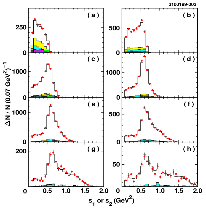
FIG. 3.: Dalitz plot projections: distributions in squared $\pi^{-}\pi^{0}$ mass $s_{1}$ and $s_{2}$ (two entries per event). The data are represented by the filled points. The solid line is the fit result. Background is represented by the shaded histograms. The lightest shaded histogram is the sum of the backgrounds, while the darker histograms show the backgrounds separately. Plots (a) to (h) correspond to slices in $\sqrt{s}=$ 0.6-0.9, 0.9-1.0, 1.0-1.1, 1.1-1.2, 1.2-1.3, 1.3-1.4, 1.4-1.5, 1.5-1.8 GeV.

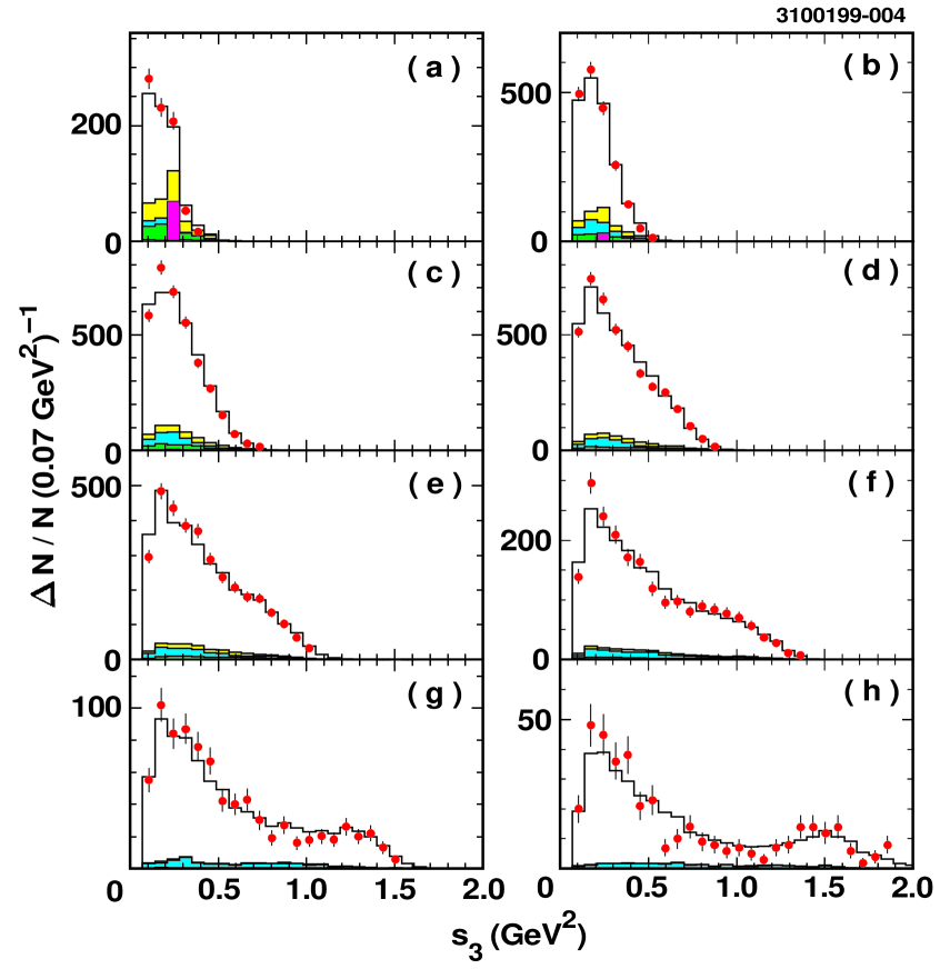
FIG. 4.: Dalitz plot projections: distributions in squared $\pi^{0}\pi^{0}$ mass $s_{3}$ (one entry per event). The data are represented by the filled points. The solid line is the fit result. Background is represented by the shaded histograms. The lightest shaded histogram is the sum of the backgrounds, while the darker histograms show the backgrounds separately. Plots (a) to (h) correspond to slices in $\sqrt{s}=$ 0.6-0.9, 0.9-1.0, 1.0-1.1, 1.1-1.2, 1.2-1.3, 1.3-1.4, 1.4-1.5, 1.5-1.8 GeV.

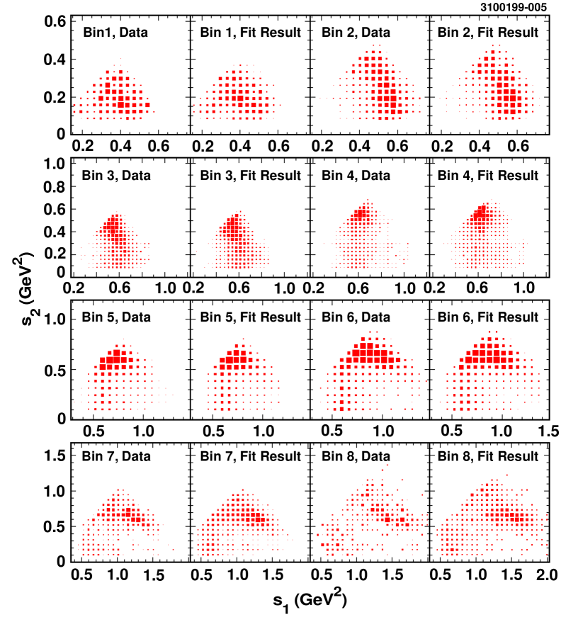
FIG. 5.: Dalitz plot distributions for data and fit result. Here $s_{1}$ is taken to be the higher of the two values of $M_{\pi^{-}\pi^{0}}^{2}$ in each event. Bins 1 through 8 correspond to slices in $\sqrt{s}=$ 0.6-0.9, 0.9-1.0, 1.0-1.1, 1.1-1.2, 1.2-1.3, 1.3-1.4, 1.4-1.5, 1.5-1.8 GeV.

D Modifications to the default model

With the model described in Section III A, we have obtained a good fit to the Dalitz plot distributions. In this section we describe fits to variations of the model.

1 Uniformity of amplitude coefficients across $\sqrt{s}$

The assumption that the coefficients $\beta_{i}$ for the various substructure amplitudes are independent of $\sqrt{s}$ may not be correct. They would not be constant if, for example, more than one $3\pi$ resonance were present. We have performed fits allowing the $\beta_{i}$ to vary; the results from one such fit are plotted in Fig. 6. In this fit, we considered fewer amplitudes so as to limit the number of fit parameters. They are $\rho\pi$ ($d$-wave), $f_{2}\pi$ ($p$-wave) and $\sigma\pi$ ($p$-wave), in addition to the dominant $s$-wave $\rho\pi$ contribution. Also, for this fit, we take the $\rho$ resonance to be the sum of $\rho(770)$ and $\rho(1450)$ amplitudes, with the $\rho(1450)$ admixture fixed according to studies of $\tau^{-}\to\nu_{\tau}\pi^{-}\pi^{0}$ decay [19]. The goodness of fit is acceptable: the measured likelihood minus that expected is $+0.2\sigma$.

The behavior of the moduli $|\beta_{i}|$ are consistent with uniformity across $\sqrt{s}$. However, we note that the signficance of the $f_{2}\pi$ contribution is greatest in the highest mass slice. We also see elevated contributions from the $\sigma\pi$ and $d$-wave $\rho\pi$ amplitudes in the high-mass slices, although these are not statistically significant.

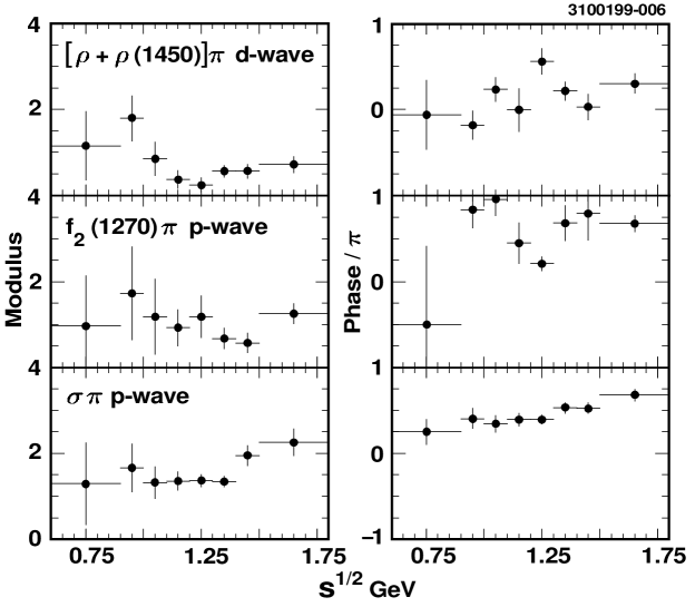
FIG. 6.: Results for the moduli and phases of coefficients $\beta_{i}$ of amplitudes from a fit in which these are allowed to vary as a function of the $3\pi$ invariant mass. In this fit, only three amplitudes are considered in addition to the $s$-wave $\rho\pi$ amplitude: $\rho\pi$ ($d$-wave), $f_{2}\pi$ ($p$-wave) and $\sigma\pi$ ($p$-wave).

2 Importance of isoscalar contributions

This analysis is the first study of the $a_{1}$ in $\tau$ decay to consider contributions from scalar $I=0$ mesons [$\sigma$ and $f_{0}(1370)$]. In addition, our fits return a significant $f_{2}(1270)\pi$ component. Although these channels are expected to be present, a demonstration of the validity of the fit results is desirable given the complexity of both the model and the fit procedure. To help visualize their collective importance in describing the substructure, we have performed fits excluding the three amplitudes $j_{5}$, $j_{6}$, and $j_{7}$ that involve isoscalars. The Dalitz plot projections from one fit performed in this way are presented in Appendix B for comparison with those from the nominal fit. We comment further on the impact of the large isoscalar contributions in Section IV F.

3 Consideration of finite size of the $a_{1}$ meson

In our nominal fit, we set the $a_{1}$ radius to zero, such that the form factors $F_{R_{i}}$ in Eqn. 5 are just unity. We find that good fits can also be obtained with non-zero values for $R_{i}$. In Fig. 7, we plot the differences in the minus log likelihood values from fits in which all $R_{i}$ are set to some value $R$. The best fit is obtained with $R=1.4\,{\rm GeV}^{-1}$. We present the results from this fit in Table VII in Appendix C. We will return to this issue in the context of the fits to the $3\pi$ mass spectrum in Section VI.

FIG. 7.: Dependence of $-2\ln{\cal L}$ on the value of the meson radius parameter $R_{i}=R$ in variations of the nominal ($R_{i}=0$) substructure fit.

4 Inclusion of $0^{-}\to 3\pi$ amplitudes

We have also performed fits including pseudoscalar contributions, namely $\pi^{\prime}\to\rho\pi$ ($p$-wave) and $\pi^{\prime}\to\sigma\pi$ ($s$-wave). These amplitudes will necessarily have a different $\sqrt{s}$-dependence from those associated with axial vector production. To account for this, we assume a Breit-Wigner form for the $\pi^{\prime}$ with a constant mass and width of 1.300 and 0.400 GeV respectively, and use the results from one of the fits presented in Section VI for the $a_{1}$ parameters.

In fits with each of these amplitudes included separately we find no statistically significant contributions. We obtain the following 90$\%$ CL limits:

$${\cal B}(\tau\to\nu\pi^{\prime}\to\nu\rho\pi\to\nu 3\pi) < 1.0\times 10^{-4},$$ (19)

$${\cal B}(\tau\to\nu\pi^{\prime}\to\nu\sigma\pi\to\nu 3\pi) < 1.9\times 10^{-4}.$$ (20)

5 Inclusion of other $1^{+}\to 3\pi$ amplitudes

In addition to the axial vector amplitudes $j^{\mu}_{1},\ldots,j^{\mu}_{7}$, we performed fits including a contribution from $f_{0}(980)\pi$ ($p$-wave). None of these fits returned a signficant coupling for this amplitude. Further discussion of possible $f_{0}(980)$ contributions appears in Section VI C 4.

6 Variation of $\sigma$ meson resonance parameters

By virtue of its low mass and large width, there is much uncertainty regarding the resonant shape of the $\sigma$ meson. For simplicity, we have elected to characterize it using a Breit-Wigner form, with its mass and width taken from the model of Törnqvist [20]. We have not considered alternative forms, or explored extensively the range of possible resonance parameters. However, in view of the large $\sigma$ contribution observed in this analysis, we have attempted to ascertain whether our data are sensitive to variation of its properties.

We have refitted the data with a range of input values for the mass and width of the $\sigma$. Of the values we considered, the best fit was obtained with $m_{0\sigma}=555$ MeV and $\Gamma_{0\sigma}=540$ MeV. The value of $-2\ln{\cal L}$ for this fit was 224216. This is 43 units below that for the nominal fit, but is still consistent with expectations given the statistics of the data sample. Using the smaller values of $m_{0\sigma}$ and $\Gamma_{0\sigma}$ has an impact on the values of $\beta_{i}$ obtained. The main trend is a relative change of 20–40$\%$ in the $a_{1}$ branching fractions, which are smaller for the $\sigma\pi$ and $f_{0}(1370)\pi$ channels and are larger for the $\rho^{\prime}\pi$ and $f_{2}(1270)\pi$ channels.

E Systematic errors

The systematic errors shown in Table III are based on estimates of the uncertainties arising from the following sources: Monte Carlo statistics, background fractions and modeling, dependence of the acceptance on the kinematical observables used in the fit, and detector resolution. The uncertainties due to these sources are given in Table IV.

TABLE IV.: Systematic errors on hadronic substructure for the nominal fit.

		$\rho(1450)$	$\rho$	$\rho(1450)$	$f_{2}(1270)$	$\sigma$	$f_{0}(1370)$
		s-wave	d-wave	d-wave	p-wave	p-wave	p-wave
	$\Delta(\mbox{${\cal B}$ fraction})$ $(\%)$	$\pm 0.162$	$\pm 0.058$	$\pm 0.045$	$\pm 0.017$	$\pm 1.201$	$\pm 0.701$
Monte Carlo	$\Delta(|\beta_{i}|)$	$\pm 0.029$	$\pm 0.028$	$\pm 0.044$	$\pm 0.047$	$\pm 0.081$	$\pm 0.049$
statistics	$\Delta(\phi_{\beta_{i}}/\pi)$	$\pm 0.038$	$\pm 0.027$	$\pm 0.058$	$\pm 0.026$	$\pm 0.011$	$\pm 0.020$
	$\Delta(\mbox{${\cal B}$ fraction})$ $(\%)$	$\pm 0.027$	$\pm 0.008$	$\pm 0.042$	$\pm 0.014$	$\pm 0.391$	$\pm 0.157$
background	$\Delta(|\beta_{i}|)$	$\pm 0.006$	$\pm 0.005$	$\pm 0.037$	$\pm 0.010$	$\pm 0.036$	$\pm 0.018$
	$\Delta(\phi_{\beta_{i}}/\pi)$	$\pm 0.005$	$\pm 0.007$	$\pm 0.018$	$\pm 0.009$	$\pm 0.007$	$\pm 0.006$
	$\Delta(\mbox{${\cal B}$ fraction})$ $(\%)$	$\pm 0.024$	$\pm 0.014$	$\pm 0.006$	$\pm 0.002$	$\pm 0.178$	$\pm 0.097$
efficiency	$\Delta(|\beta_{i}|)$	$\pm 0.004$	$\pm 0.007$	$\pm 0.008$	$\pm 0.002$	$\pm 0.016$	$\pm 0.007$
	$\Delta(\phi_{\beta_{i}}/\pi)$	$\pm 0.013$	$\pm 0.002$	$\pm 0.009$	$\pm 0.001$	$\pm 0.006$	$\pm 0.008$
	$\Delta(\mbox{${\cal B}$ fraction})$ $(\%)$	$\pm 0.018$	$\pm 0.006$	$\pm 0.004$	$\pm 0.002$	$\pm 0.083$	$\pm 0.065$
detector	$\Delta(|\beta_{i}|)$	$\pm 0.001$	$\pm 0.002$	$\pm 0.007$	$\pm 0.001$	$\pm 0.011$	$\pm 0.006$
resolution	$\Delta(\phi_{\beta_{i}}/\pi)$	$\pm 0.002$	$\pm 0.004$	$\pm 0.006$	$\pm 0.002$	$\pm 0.004$	$\pm 0.005$
	$\Delta(\mbox{${\cal B}$ fraction})$ $(\%)$	$\pm 0.17$	$\pm 0.06$	$\pm 0.06$	$\pm 0.02$	$\pm 1.28$	$\pm 0.73$
total	$\Delta(|\beta_{i}|)$	$\pm 0.03$	$\pm 0.03$	$\pm 0.06$	$\pm 0.05$	$\pm 0.09$	$\pm 0.05$
	$\Delta(\phi_{\beta_{i}}/\pi)$	$\pm 0.04$	$\pm 0.03$	$\pm 0.06$	$\pm 0.03$	$\pm 0.02$	$\pm 0.02$

The error due to Monte Carlo statistics is based on the variance of results obtained from six separate fits, each using one sixth of the Monte Carlo sample for the normalization of the likelihood function. Fits performed after varying the background fractions and model (in the case of the $\nu_{\tau}\,\pi^{-}\,3\pi^{0}$ channel) within reasonable limits were used to estimate the error associated with this source. To estimate the error associated with acceptance, the Monte Carlo was used to parameterize acceptance as a function of the charged and neutral pion momenta as well as the opening angles between these particles. Reasonable deviations from these parameterizations were used to reweight events entering the fit, and the resulting variations in fit parameters were taken as the systematic errors. Finally, the likelihood function in Eqn. 15 does not take into account resolution effects. The effects of modifying it to include resolution smearing based on errors in track parameters for the $\pi^{-}$ and in photon energies and directions for the $\pi^{0}$’s was used to estimate the error from this source. For all fit parameters, the error due to limited Monte Carlo statistics dominates the systematic error.

The results given in Table III are meaningful only in the context of the model used to parametrize the substructure. Different models yield results that can differ significantly from our nominal fit results. Given this plus the unfeasibility of examining all possible models, we have not attempted to assign a systematic error associated with model dependence.

F Discussion

The results of the fits for the substructure can be summarized as follows:

• The $\rho\pi$ $s$-wave amplitude with a branching fraction of around $70\%$ is dominant, as expected.

• With the exception of the $\rho(1450)\pi$ $s$-wave amplitude, all amplitudes included in the nominal fit contribute significantly to the $3\pi$ hadronic current. In other fits, we find no evidence for contributions from $a_{1}\to f_{0}(980)\pi$, or from $\tau^{-}\to\nu_{\tau}\pi^{\prime-}$.

• The isoscalar mesons $f_{2}$, $f_{0}(1370)$, and $\sigma$ contribute with a combined branching fraction of approximately $20\%$ to the $3\pi$ hadronic width. In particular, the $\sigma$ meson with a significance of $\sim 8\sigma$ cannot be neglected. It shows up strongly as part of the broad enhancement at the low end in the $s_{3}$ ($M_{\pi^{0}\pi^{0}}^{2}$) distribution in the slices of $\sqrt{s}$ shown in Fig. 4(g) and (h), but is significant in all slices.

• The $\rho(1450)\pi$ state shows up more strongly in the $d$-wave amplitude than in the $s$-wave amplitude.

The last point above may have implications regarding a possible $a_{1}^{\prime}$ contribution. One expects that an $a_{1}^{\prime}$ contribution induces $\sqrt{s}$-dependent couplings. In the fits allowing $\beta_{i}$ to vary with $\sqrt{s}$, we found that (1) the goodness of fit is not significantly better, and (2) the values of $\beta_{i}(s)$ are roughly consistent with being constant. On the other hand, according to the flux-tube-breaking model of Refs. [21, 22], the $a_{1}^{\prime}$ meson prefers to decay to $\rho\pi$ by $D$-wave rather than $S$-wave, and the $\rho(1450)$ is preferred over the $\rho(770)$. Thus, it is possible that the measured $\rho(1450)\pi$ $d$-wave amplitude could be induced by an $a_{1}^{\prime}$. The suggestions of enhanced $f_{2}\pi$ and $\sigma\pi$ contributions at large $\sqrt{s}$ are also consistent with the hypothesis of an $a_{1}^{\prime}$. However, the statistics of the present data sample are not sufficient to resolve this question with the substructure fits.

As a test of our fit results, we have compared the Dalitz plot distributions from a sample of background-subtracted $\tau^{-}\rightarrow\nu_{\tau}\pi^{-}\pi^{-}\pi^{+}$ events with the isospin prediction based on the results from the nominal fit to the $\pi^{-}\pi^{0}\pi^{0}$ mode. The backgrounds were estimated from the generic $\tau$ Monte Carlo sample. The dominant backgound $\tau^{-}\to\nu_{\tau}\pi^{-}\pi^{-}\pi^{+}\pi^{0}$ is simulated in this sample with the model implemented in TAUOLA, containing $\pi^{-}\omega$ as well as $[\rho\pi\pi]^{-}$ (in various charge combinations) substructure. The Dalitz plot projections are shown in Fig. 8. The observation that the hadronic current for the all-charged mode is well described by our results for the $\pi^{-}\pi^{0}\pi^{0}$ mode provides a critical corroboration of our measurements. This is particularly important for the amplitudes involving isoscalars since they enter the all-charged mode with the opposite sign relative to the other amplitudes. A full analysis of the high-statistics all-charged mode is under way and will be presented in the future.

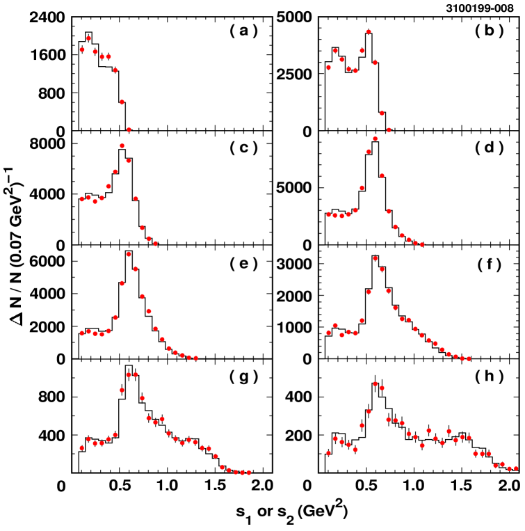
FIG. 8.: Background-subtracted squared $\pi^{+}\pi^{-}$ mass ($s_{1}$ and $s_{2}$) spectrum for the three charged pion mode (two entries per event). The data are represented by the filled points. The solid line is the isospin prediction based on our fit to the $\pi^{-}\pi^{0}\pi^{0}$ mode.

The world average values [1] for the $\tau^{-}\to\nu_{\tau}\pi^{-}\pi^{+}\pi^{-}$ and $\tau^{-}\to\nu_{\tau}\pi^{-}\pi^{0}\pi^{0}$ branching fractions are $(9.23\pm 0.11)\,\%$ and $(9.15\pm 0.15)\,\%$, respectively. Their near equality is consistent with expectations from isospin symmetry, if the decays were to proceed exclusively via $\rho\pi$ or $\rho^{\prime}\pi$. One consequence of the presence of isoscalars in $a_{1}$ decay is the possibility of upsetting this expectation. However, due to interference the two modes contribute nearly equally to $\Gamma^{a_{1}}_{tot}(s)$ (see Fig. 9(b) in Section VI B). The divergence of these contributions at high values of $\sqrt{s}$ is damped in the decay rate by the falling of the $a_{1}$ line shape, as well as by phase space and weak interaction dynamics in the $\tau$ decay. Furthermore, the residual preference for the all-charged mode at high $\sqrt{s}$ is compensated for by the larger phase space available for the $\pi^{-}2\pi^{0}$ mode at low $\sqrt{s}$. Quantitatively, the ratio of branching fractions is predicted from this analysis to be ${\cal B}(\tau^{-}\to\nu_{\tau}\pi^{-}\pi^{+}\pi^{-})/{\cal B}(\tau^{-}\to\nu_{\tau}\pi^{-}\pi^{0}\pi^{0})=0.985$, in agreement with the ratio $1.009\pm 0.020$ obtained from the direct measurements.

Finally, the branching fractions reported in Table III are the $\tau^{-}$ decay branching fractions relative to the total $\nu_{\tau}\pi^{-}\pi^{0}\pi^{0}$ rate. These differ from the $a_{1}$ branching fractions due to the weighting of the $a_{1}$ line shape by factors associated with $\tau^{-}\to\nu_{\tau}a_{1}^{-}$ weak decay. The $a_{1}$ branching ratios ${\cal B}(a_{1}^{-}\to[Y\pi]^{-}\to\pi^{-}\pi^{0}\pi^{0})/{\cal B}(a_{1}^{-}\to\pi^{-}\pi^{0}\pi^{0})$ are given in Table V.

TABLE V.: Branching ratios for $a_{1}^{-}$ decay into $\pi^{-}\pi^{0}\pi^{0}$ via intermediate states shown, relative to the total $a_{1}^{-}\to\pi^{-}\pi^{0}\pi^{0}$ rate. The errors shown are statistical only.

Amplitude		Branching ratio $(\%)$
$\rho\pi$	$s$-wave	$60.19$
$\rho(1450)\pi$	$s$-wave	$\phantom{1}0.56\pm 0.84$
$\rho\pi$	$d$-wave	$\phantom{1}1.30\pm 0.60$
$\rho(1450)\pi$	$d$-wave	$\phantom{1}2.04\pm 1.20$
$f_{2}(1270)\pi$	$p$-wave	$\phantom{1}1.19\pm 0.49$
$\sigma\pi$	$p$-wave	$18.76\pm 4.29$
$f_{0}(1370)\pi$	$p$-wave	$\phantom{1}7.40\pm 2.71$

V DETERMINATION OF THE SIGNED $\nu_{\tau}$ HELICITY

In the fits reported in the previous section, the $\tau$ neutrino (anti-neutrino) helicity was fixed to the Standard Model value of $h_{\nu_{\tau}}=-1$ ($h_{\overline{\nu}_{\tau}}=+1$). However as first pointed out by Kühn and Wagner [25], interference between the two $\pi^{-}\pi^{0}$ systems gives rise to a parity violating term in the squared matrix element for the decay $\tau^{-}\to\nu_{\tau}\pi^{-}\pi^{0}\pi^{0}$. This permits determination of the sign, as well as the magnitude, of the neutrino helicity. Including $h_{\nu_{\tau}}$ as an additional free parameter to the nominal fit described in the previous section, and assuming invariance under the combined charge-conjugation and parity ($CP$) operation, we find $h_{\nu_{\tau}}=-1.00\pm 0.12$. In this fit, the values of $\beta_{i}$ are affected at a negligible level. Including only the $s$-wave $\rho\pi$ amplitude in the model for the substructure yields a poor fit, with $h_{\nu_{\tau}}=-0.73\pm 0.09$.

To investigate the model dependence entering this measurement we also performed fits for substructure and $h_{\nu_{\tau}}$ with different input parameters. While our nominal fit was performed with the $a_{1}$ radius set to zero, non-zero values also gave good fits, as noted in the previous section. Using the best fit value of $R_{i}=1.4\mbox{ GeV}^{-1}$, we obtain $h_{\nu_{\tau}}=-1.03\pm 0.13\,.$ As a best estimate of $h_{\nu_{\tau}}$ given the dependence on input assumptions, we average this value with the $R_{i}=0$ result to obtain

$$h_{\nu_{\tau}}=-1.02\pm 0.13\,\mbox{\sl(stat.)}\pm 0.01\,\mbox{\sl(syst.)}\pm 0.03\,\mbox{\sl(model)}\,,$$ (21)

where the uncertainty due to the model dependence is estimated by the difference between the values from these two fits. This result agrees with other determinations [1] of the sign and magnitude of $h_{\nu_{\tau}}$, as well as with the Standard Model value of $-1$.

The systematic error given for $h_{\nu_{\tau}}$ was determined in a fashion similar to those in the substructure analysis. The sources contributing to this error are: Monte Carlo statistics ($\pm 0.005$), background determination ($\pm 0.010$), dependence of the acceptance on the kinematic observables used in the fit ($\pm 0.003$), and detector resolution ($\pm 0.004$).

We have also looked for possible $CP$ non-conservation by determining $h_{\nu_{\tau}}$ and $h_{\overline{\nu}_{\tau}}$ separately. Defining a $CP$-violating asymmetry

$$A_{CP}=\frac{h_{\overline{\nu}_{\tau}}+h_{\nu_{\tau}}}{|h_{\overline{\nu}_{\tau}}|+|h_{\nu_{\tau}}|},$$ (22)

we find $A_{CP}=-0.08\pm 0.13$, where the error is dominantly due to statistics.

VI ANALYSIS OF THE $\pi^{-}\pi^{0}\pi^{0}$ MASS SPECTRUM

In this section, we describe fits to the $3\pi$ mass spectrum performed to extract resonance parameters of the $a_{1}$ meson. The results from the substructure fits are used as inputs for determination of the running of the $a_{1}$ mass and width.

A Fitting method and assumptions

The $a_{1}$ resonance parameters are determined from a $\chi^{2}$ fit to the background-subtracted and efficiency-corrected $\pi^{-}\pi^{0}\pi^{0}$ mass spectrum. The fit is performed over a range from $M_{3\pi}=0.600$ to 1.725 GeV in bins of width 25 MeV. As in the substructure analysis, we perform a variety of fits, reflecting different models and assumptions. We perform fits to the all-tagged sample, as well as to the lepton-tagged subsample, to benefit from the higher statistics.

For our nominal fit, we specify the following version of the model described in Section III B: (1) turn off $a_{1}^{\prime}$ contribution, i.e., set $\kappa=0$ in Eqn. 7; (2) turn off form factors describing finite size of the $a_{1}$, i.e., set $R_{i}=0$; (3) include the $K^{*}K$ threshold, but not the $f_{0}(980)\pi$ threshold, in determining $\Gamma^{a_{1}}_{tot}(s)$; and (4) assume the running $a_{1}$ mass to be flat as a function of $\sqrt{s}$. We have also performed fits in which various of these specifications are modified, and obtain satisfactory results under a variety of configurations. With the above specifications, the fit contains three free parameters in addition to an overall normalization: the pole $a_{1}$ mass $m_{0a_{1}}$, the $a_{1}\to 3\pi$ coupling $g_{a_{1}(3\pi)}$, and the relative $a_{1}\to K^{*}K$ coupling $\gamma_{a_{1}(K^{*}K)}$. We derive from these parameters the pole $a_{1}$ width $\Gamma_{0a_{1}}$ using Eqn. 12.

Some comments on the above choices are in order. The $\sqrt{s}$-dependence of the $a_{1}$ total width depends strongly on assumptions. Inclusion of the $K^{*}K$ channel is motivated by observation of the decay $\tau^{-}\to\nu_{\tau}[K^{*}K]^{-}$ [1], although it is not well-determined as to how much of this comes through the axial vector (rather than vector) weak current. As we have no evidence for the $f_{0}(980)\pi$ channel in the substructure fits, we have omitted its possible contribution in our nominal fit here. However, this and other thresholds may be present. For example, a possible $a_{1}\to f_{1}(1285)\pi$ channel, as suggested by the recent obervation of this system in $\tau$ decay [15], would open up near the $K^{*}K$ threshold. Thus, the value for $\Gamma^{a_{1}}_{K^{*}K}$ returned from our fit can not be strictly interpreted as just the $a_{1}\to K^{*}K$ partial width.

The running of the $a_{1}$ mass is even more problematic since the upper limit of integration (over $ds^{\prime}$) in Eqn. 10 is infinity, and thus the integral will include effects from channels that open above the $\tau$ mass, and are therefore not directly measureable in $\tau$ decay. Furthermore, a damping of the amplitudes, such as that provided by the form factors $F_{R_{i}}$, is needed so that the integral can converge. As a result, allowing the $a_{1}$ mass to run is practical only in models where the $R_{i}$ are non-zero. In such models, the effect of additional thresholds at high $\sqrt{s}$ is to flatten the $\sqrt{s}$-dependence of the running mass. Thus, we expect the running mass to be closer to a constant than we would predict from Eqn. 9 with known thresholds. Setting $R_{i}=0$ and taking a constant $a_{1}$ mass may not be rigorous, however the resulting model is simplified.

B Results

The results obtained from our nominal fit to the $3\pi$ resonance shape parameters are shown in the second column of Table VI. The $\chi^{2}$ for this fit is 39.3 for 41 degrees of freedom. Fits to just the lepton-tagged event sample yield consistent results.

The background-subtracted, efficiency-corrected $3\pi$ mass spectrum from the all-tagged sample is shown in Fig. 9(a), with the function corresponding to the nominal fit overlaid. Shown in Fig. 9(b) is the $a_{1}$ width $\Gamma_{tot}^{a_{1}}(s)$, as defined by Eqn. 12, as well as the contributions from the individual $a_{1}$ decay channels considered. The kink associated with the turn-on of $a_{1}\to K^{*}K$ is visible in the $3\pi$ mass spectrum at $\sim 1.375$ GeV.

TABLE VI.: Results for fits to the $3\pi$ resonance shape, with nominal background and efficiency correction. The second column gives results based on the nominal fit function. The first error is that due to statistics, while the second is the systematic error. The third column gives results from the fit including an $a_{1}^{\prime}$ contribution, with statistical errors only. The derived quantity ${\cal B}(K^{*}K)$, the $a_{1}\to K^{*}K$ branching fraction, is also shown assuming this is the only amplitude accounted for by the threshold function labeled $\Gamma_{K^{*}K}$ in Fig. 9(b) (see text). The quantity $\phi_{\kappa}$ denotes the phase of the $a_{1}^{\prime}$ amplitude relative to that of the $a_{1}$.

Fit Parameter	Nominal Fit	Fit with $a_{1}^{\prime}$
$m_{0a_{1}}\mbox{ (GeV)}$	$1.331\pm 0.010\pm 0.003$	$1.330\pm 0.011$
$\Gamma_{0a_{1}}\mbox{ (GeV)}$	$0.814\pm 0.036\pm 0.013$	$0.814\pm 0.038$
$\gamma_{a_{1}(K^{\star}K)}$	$3.32\pm 0.26\pm 0.04$	$3.72\pm 0.45$
${\cal B}(K^{\star}K)$ $(\%)$	$3.3\pm 0.5\pm 0.1$	$4.0\pm 1.0$
$|\kappa|$	0	$0.053\pm 0.019$
$\phi_{\kappa}/\pi$	—	$0.10\pm 0.22$
$\chi^{2}/ndof$	$39.3/41$	$28.9/39$

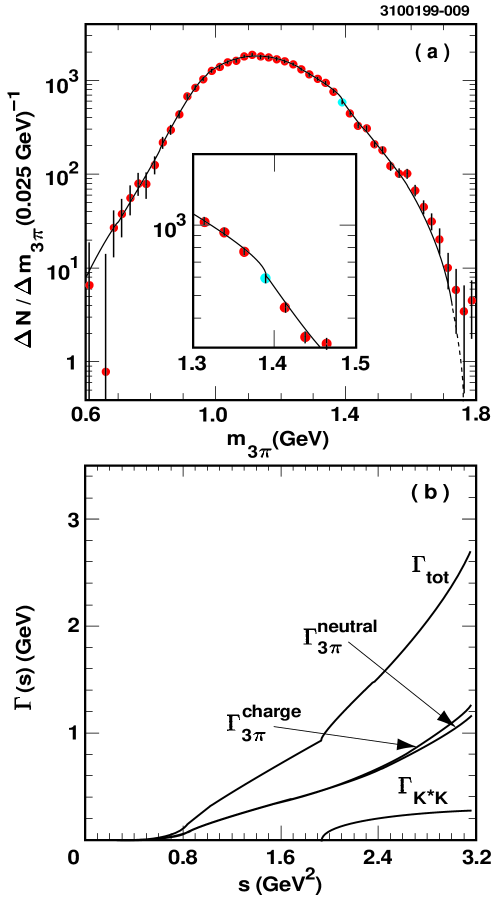
FIG. 9.: (a) Background-subtracted, efficiency-corrected $3\pi$ mass spectrum from the all-tag sample. The solid line shows the result from the nominal fit. The inset shows a magnified view of the $a_{1}\to K^{*}K$ threshold region. In (b), the $\sqrt{s}$-dependent $a_{1}$ width $\Gamma_{tot}^{a_{1}}(s)$ is plotted as a function of $s$, along with the separate contributions from the channels considered, as given in Eqn. 12. The labels $\Gamma^{\rm charge}_{3\pi}$ and $\Gamma^{\rm neutral}_{3\pi}$ refer to the contributions from the $a_{1}^{-}\to\pi^{-}\pi^{+}\pi^{-}$ and $\pi^{-}\pi^{0}\pi^{0}$ channels respectively.

C Modifications to the nominal fit function

1 Finite size of the $a_{1}$ meson

Like the Dalitz plot distributions, the $3\pi$ mass spectrum contains some sensitivity to the parametrization of the $a_{1}$ as being point-like or of finite size. Here the sensitivity depends also on the treatment of the $\sqrt{s}$-dependence of $a_{1}$ mass.

As in the substructure analysis, we re-fit the data multiple times, stepping through a range of values for the $a_{1}$ meson size parameter $R$. The results from these fits are given in Appendix C. For both the all-tag and lepton-only-tag samples, the best fits were obtained with values of $R$ between 1.2 and 1.4 GeV^-1, depending on whether the $a_{1}$ mass was treated as a running or constant mass. This agrees well with the substructure analysis which favors a value of $R$ of 1.4 GeV^-1. This value of $R$ corresponds to an r.m.s. radius of the $a_{1}$ of 0.7 fm. It is interesting to note that this is similar to the value employed by Isgur, Morningstar and Reader citeIMR in their analysis of the $3\pi$ line shapes from the DELCO [26], MARK II [27] and ARGUS [28] experiments. However, the statistics of the present sample are not sufficient to determine the necessity of including the $F_{R}(k)$ form factor in the parametrization of the hadronic current.

Despite this, uncertainty on this issue represents a substantial source of model dependence with regard to the $a_{1}$ resonance parameters. Tables VIII and IX in Appendix C demonstrate this point. As an example, for $R=1.2\,\mbox{GeV}^{-1}$ with a constant $a_{1}$ mass, we find $m_{0a_{1}}=1.285\pm 0.007$ GeV and $\Gamma_{0a_{1}}=0.619\pm 0.021$ GeV (statistical errors only).

2 Running of the $a_{1}$ mass

As indicated above, we have also performed fits with the $\sqrt{s}$-dependence of the $a_{1}$ mass computed according to Eqn. 9. This can only be done in models with non-zero values for the $a_{1}$ size parameter $R$. The results, also given in Appendix C, indicate that slightly better fits can be obtained using a running $a_{1}$ mass. However, since satisfactory fits are obtained with a constant mass, we conclude that the present data sample is not sensitive to the running of the $a_{1}$ mass.

3 Inclusion of an $a_{1}^{\prime}(1700)$ admixture

Despite the goodness of the fit to the nominal model, the data above 1.575 GeV show an excess relative to the fit function in Fig. 9. This region is where contributions from interference with an $a_{1}^{\prime}$ meson with mass around 1.7 GeV might appear. We have performed various fits allowing $\kappa$ in Eqn. 7 to float. The results from one such fit are given in the last column of Table VI and plotted in Fig. 10(a). In this fit, we have used $m_{0a_{1}^{\prime}}=1.700$ GeV and $\Gamma_{0a_{1}^{\prime}}=0.300$ GeV. We have also fixed the $a_{1}^{\prime}(\rho^{\prime}\pi)$ coupling to be equal to the $a_{1}^{\prime}(\rho\pi)$ coupling to determine $\Gamma_{a_{1}^{\prime}}(s)$ as shown in Fig. 10(b). This is an ad hoc choice, however the fit is relatively insensitive to the parametrization of $\Gamma_{a_{1}^{\prime}}(s)$.

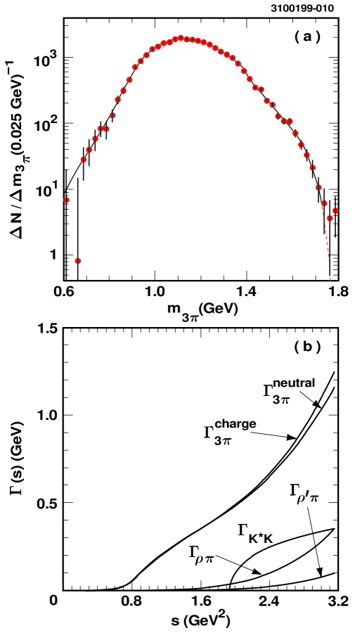
FIG. 10.: (a) Background-subtracted, efficiency-corrected $3\pi$ mass spectrum from the all-tag sample. The solid line shows the fit result for the model in which an $a_{1}^{\prime}$ admixture is allowed to contribute. In (b) the assumed $\rho\pi$ and $\rho^{\prime}\pi$ contributions to the $a_{1}^{\prime}$ width in this model are shown, along with the contributions to the $a_{1}$ width from Fig. 9 for comparison.

The $\chi^{2}$ for this fit is 28.9 for 39 degrees of freedom. The $a_{1}^{\prime}$ contribution has a significance of 2.8$\sigma$, with $|\kappa|=0.053\pm 0.019$ and a phase $\phi_{\kappa}$ consistent with zero. If we take $\phi_{\kappa}$ to be zero, the resulting fit yields $|\kappa|=0.060\pm 0.017$. To test whether backgrounds in the all-tag sample are influencing this result, we have also fit the spectrum from just the lepton-tag events (with $\phi_{\kappa}$ floating). This fit yields consistent results, with $|\kappa|=0.05\pm 0.04$.

The analysis of DELPHI [12] yielded a large amplitude for the $a_{1}^{\prime}$ contribution, with $|\kappa|$ in the range of $0.50\pm 0.06$ to $0.75\pm 0.06$, depending on the model used. The corresponding values obtained here are smaller by an order of magnitude, and are much less significant statistically. However, the models used by DELPHI include neither the contributions to $\Gamma^{a_{1}}_{tot}(s)$ from the opening of the $K^{*}K$ channel, nor those associated with the isoscalar channels. In particular, the $K^{*}K$ amplitude has a significant effect at large values of $\sqrt{s}$ where the spectrum is most sensitive to the presence of an $a_{1}^{\prime}$. Omitting the $K^{*}K$ amplitude in our fit, we obtain a value of $|\kappa|$ approximately twice as large as our nominal value. Finally, the DELPHI anaylsis involves a simultaneous fit to the $3\pi$ mass spectrum and the Dalitz plot projections at large $\sqrt{s}$, employing assumptions for the substructure composition that differ from what we have determined (for the $a_{1}$) in our substructure analysis. In summary, direct comparison of our value of $\kappa$ with that from the DELPHI analysis is not meaningful.

4 Opening of $f_{0}(980)\pi$ threshold

Since the impact of the opening of $K^{*}K$ threshold appeared to be significant, we also performed fits including the opening of $f_{0}(980)\pi$ threshold. This would include contributions through both $f_{0}\to\pi\pi$ and $K\overline{K}$ channels. The $f_{0}\to\pi^{0}\pi^{0}$ channel would be expected to contribute to the substructure in our $\pi^{-}\pi^{0}\pi^{0}$ sample, but the other modes would not do so.

Marginal improvements in the fit quality were obtained only for those models in which the $a_{1}$ mass was run according to Eqn. 9. In these cases the $f_{0}(980)\pi$ contributions to the total width of the $a_{1}$ were present at the $2\sigma$ level or less. Fits including this contribution are discussed in Appendix C.

To summarize, we find no evidence for contribution from the opening of the $a_{1}\to f_{0}(980)\pi$ channel in either the substructure fits or the $3\pi$ mass fits. However, other scalar $I=0$ mesons [$\sigma$ and $f_{0}(1370)$] are needed to provide a good description of the substructure. This observation may have some bearing on the interpretation of the $f_{0}(980)$ as something other than a $q\overline{q}$ meson, as has been frequently speculated (see for example Ref. [1]). Given the theoretical and experimental complexity, we cannot comment on this issue except to note that the non-observation of the $f_{0}(980)$ in $a_{1}$ decay is not inconsistent with an exotic interpretation for this state.

D Systematic errors

The sources of the systematic errors shown in Table VI are just those associated with background subtraction and acceptance. The background errors are estimated by repeating the fit after separately varying the amount of each of the backgrounds being subtracted. We vary the background fractions of modes with two real $\pi^{0}$’s by three times the uncertainty on their branching fractions. In the case of the fake-$\pi^{0}$ background, the subtraction is varied by three times the statistical error of the $\pi^{0}\pi^{0}$ side band sample. Finally, the $\sqrt{s}$-dependence of the acceptance as determined from Monte Carlo events is parametrized; these parameters are then varied by three standard deviations to estimate the associated uncertainty.

The systematic errors shown in Table VI are dominated by the errors due to the background subtraction. As a check, we have performed fits allowing the separate background normalization and acceptance correction functions to float, subject to constraints added to the $\chi^{2}$ on the magnitude of their deviations from nominal. The changes in fit parameters observed in these fits are small relative to the quoted errors. The deviations of the correction functions from nominal are also small in this fit. As in the substructure fits, we do not assign a systematic error for model dependence.

E Discussion

As can be seen from Fig. 9(a), and from the $\chi^{2}$ for the nominal fit shown, the model described in Sec. III B, with the assumptions listed in Sec. VI A, provides a good description of the data. The $a_{1}$ pole mass and width are determined precisely, however their values depend significantly on the model and input assumptions.

The results demonstrate the importance of including the opening of $K^{*}K$ threshold. Fits performed without this contribution to $\Gamma^{a_{1}}_{tot}(s)$ yield large $\chi^{2}$ values. The obtained $a_{1}\to K^{*}K$ branching fraction $(3.3\pm 0.5)\%$ corresponds to a $\tau$ branching fraction of ${\cal B}(\tau^{-}\to\nu_{\tau}a_{1}^{-}\to\nu_{\tau}[K^{*}K]^{-})=(0.16\pm 0.03)\%$. For comparison, multiplying the directly measured $\tau^{-}\to\nu_{\tau}K^{*0}K^{-}$ branching fraction [1] by a factor of two (to account for $K^{*-}K^{0}$) gives ${\cal B}(\tau^{-}\to\nu_{\tau}[K^{*}K]^{-})=(0.42\pm 0.08)\%$. The apparent shortfall in our measurement is not surprising since the $\nu_{\tau}[K^{*}K]^{-}$ final state is expected to receive contributions from both vector and axial vector hadronic currents.

In the high-mass region above 1.575 GeV, the data appear to be systematically high relative to the fit function. To understand whether this is an experimental effect, we have modified the background and efficiency corrections within reasonable limits. As described in the previous section, we have also performed fits in which background and efficiency correction functions are allowed to float. Neither of these approaches significantly improves the fit in this region. Fits with non-zero values of $R_{i}$, with and without a running $a_{1}$ mass, and/or including the $f_{0}(980)\pi$ threshold also fail in this respect.

Including a contribution from an $a_{1}^{\prime}$ meson, however, visibly influences the shape of the $3\pi$ mass spectrum in the high-mass region, as shown in Fig. 10(a). As noted earlier, the presence of an $a_{1}^{\prime}$ may also be consistent with an enhanced $d$-wave contribution from $\rho(1450)\pi$ relative to $s$-wave, as observed in the substructure analysis. We have not evaluated systematic errors associated with the $a_{1}^{\prime}$ contribution determined from the $3\pi$ mass spectrum fits, since these are likely dominated by uncertainties associated with the modeling of the $a_{1}$ line shape. We have performed other fits with an $a_{1}^{\prime}$, sampling the range of model variations described above. The statistical significance of the $a_{1}^{\prime}$ contribution is typically 2-3$\,\sigma$ in these fits. We conclude that more data is needed to establish whether the $a_{1}^{\prime}$ is present.

VII SUMMARY AND CONCLUSIONS

To summarize, we have presented a detailed model-dependent analysis of hadronic structure in the decay $\tau^{-}\to\nu_{\tau}\pi^{-}\pi^{0}\pi^{0}$ using data obtained with the CLEO II detector. This decay mode represents a unique source of information on the $I=1$ axial vector meson sector, an area of hadron spectroscopy which is difficult to access cleanly via other production mechanisms. In this analysis we have derived successful descriptions of both the $a_{1}$ line shape and the substructure present in its decay to three pions. The most significant result is the observation of large contributions to the substructure from intermediate states involving the isoscalar mesons $\sigma$, $f_{0}(1370)$, and $f_{2}(1270)$. With this, our data also provides new input on the complicated $I=0$ scalar meson sector: we observe some sensitivity to the properties of the $\sigma$ meson, for example. More generally, significant progress towards a satisfactory description of Dalitz plot distributions in $\tau^{-}\to\nu_{\tau}[3\pi]^{-}$ decay has been achieved. This is supported by the observation that our characterization of substructure in the $\nu_{\tau}\pi^{-}\pi^{0}\pi^{0}$ mode also provides a good description of substructure in the $\nu_{\tau}\pi^{-}\pi^{+}\pi^{-}$ data.

Using the results from the substructure fits to infer the $\sqrt{s}$-dependence of the $a_{1}$ width, we have determined the $a_{1}$ meson resonance parameters. We obtain $m_{0a_{1}}=1.331\pm 0.010\pm 0.003$ GeV and $\Gamma_{0a_{1}}=0.814\pm 0.036\pm 0.013$ GeV, although these values depend significantly on the details of the model used to fit the $3\pi$ mass spectrum. For example, taking the meson size parameter to be $R=1.2\,\mbox{GeV}^{-1}$ instead of zero, we find $m_{0a_{1}}=1.285\pm 0.007\,\mbox{(stat.)}$ GeV and $\Gamma_{0a_{1}}=0.619\pm 0.021\,\mbox{(stat.)}$ GeV. Such model dependences are not reflected in the quoted systematic errors. We also find a significant contribution to the $\sqrt{s}$-dependence of the $a_{1}$ width associated with the opening of the $a_{1}\to K^{*}K$ decay channel at high values of $\sqrt{s}$.

We have investigated the possibility of an additional contribution to the $3\pi$ mass spectrum from a radially excited $a_{1}^{\prime}$ meson, as suggested by the analysis of DELPHI [11, 12]. This is also suggested by our data, which show an apparent excess of events at large $3\pi$ mass relative to various fits without an $a_{1}^{\prime}$ component. The data are better described with an $a_{1}^{\prime}$ contribution, though at a level below that reported by DELPHI. The model used in our analysis differs substantially from that analysis, with regard to treatment of the $K^{*}K$ threshold and the substructure in the $a_{1}\to 3\pi$ channel. We have not assessed the impact on $\nu_{\tau}$ mass studies of effects associated with the complex substructure in $a_{1}\to 3\pi$ decay or the apparent distortions in the $3\pi$ mass spectrum caused by the $K^{*}K$ and possible $a_{1}^{\prime}$ contributions. However, careful consideration of such effects in the course of these analyses should improve the reliability of the ensuing tau neutrino mass constraints.

We have also obtained a precise determination of the signed $\tau$ neutrino helicity $h_{\nu_{\tau}}=-1.02\pm 0.13\;(\mbox{stat.})\pm 0.03\;(\mbox{syst.}+\mbox{model})$ when this quantity is left as a free parameter in the substructure fits. As has been noted in earlier measurements of this quantity [8], accurate parameterization of the substructure is important for obtaining an unbiased measurement. With the improved understanding of this substructure, this result provides unambiguous evidence for the left-handedness of the $\tau$ neutrino.

We have addressed several additional issues pertaining to the characterization of axial vector meson decay dynamics. For example, the data show limited sensitivity to the finite size of the $a_{1}$ meson, both in the substructure and the $3\pi$ mass spectrum fits. With the parametrization of the associated form factor used here, we find that both analyses favor an r.m.s. $a_{1}$ radius of around 0.7 fm. As with the question of a possible $a_{1}^{\prime}$ contribution, a definitive conclusion on this issue requires additional data. We have looked for indications of non-axial-vector contributions to the $3\pi$ substructure via the $\pi^{\prime}(1300)$ resonance, and have placed upper limits on the $\tau$ decay rate to this state. Detailed analyses of the higher-statistics $\tau^{-}\to\nu_{\tau}\pi^{-}\pi^{+}\pi^{-}$ data should shed additional light on these and other issues.

Although the quantitative results presented in this article are strongly model-dependent, they describe successfully the qualitative features of the data. However, further insight can be gained from a quantitative model-independent analysis of the data, such as that proposed by Kühn and Mirkes [29]. We are presently pursuing such an analysis and will report the results in a separate article.

A PARAMETERIZATION OF SUBSTRUCTURE IN $\tau^{-}\to\nu_{\tau}\pi^{-}\pi^{0}\pi^{0}$

To parameterize the model used to fit for the substructure in $\tau^{-}\to\nu_{\tau}\pi^{-}\pi^{0}\pi^{0}$, we follow many of the conventions used in the KORALB/TAUOLA [17] $\tau\tau$ Monte Carlo generator. We first denote the four-momenta of the pions by

$$p_{1} = \pi^{0}_{1}$$ four-momentum of , (A1)

$$p_{2} = \pi^{0}_{2}$$ four-momentum of , and (A2)

$$p_{3} = \pi^{-}$$ four-momentum of . (A3)

We then define the quantities $q_{1}=p_{2}-p_{3}$, $q_{2}=p_{3}-p_{1}$, $q_{3}=p_{1}-p_{2}$, and $a=p_{1}+p_{2}+p_{3}$. Ignoring for now the resonant structure of the $3\pi$ system, the general form for $3\pi$ hadronic current $J^{\mu}$ as defined by Eqs. 1 and 2 can be written as:

$$J^{\mu}=T^{\mu\nu}\left[c_{1}q_{1\nu}F_{1}+c_{2}q_{2\nu}F_{2}+c_{3}q_{3\nu}F_{3}\right]+c_{4}a^{\mu}F_{4}+c_{5}i\epsilon^{\mu\nu\rho\sigma}p_{1\nu}p_{2\rho}p_{3\sigma}F_{5}\,,$$ (A4)

where the $c_{i}$ are complex scalar coefficients, and $T^{\mu\nu}=g^{\mu\nu}-{a^{\mu}a^{\nu}}/{a^{2}}$.

The form factors $F_{i}$ contain the description of the low energy QCD phenomena we are studying. Owing to Lorentz invariance, they depend only on Lorentz scalars. The terms containing $F_{1}$, $F_{2}$ and $F_{3}$ are associated with the axial vector contribution. The term containing $F_{3}$ is not needed since it can be absorbed into the terms containing $F_{1}$ and $F_{2}$. We write it explicitly here to make connection with form factors associated with specific resonant substructure. $F_{4}$ is the scalar form factor, and $F_{5}$ is the $G$-parity violating vector form factor. Neither of these are expected to contribute significantly in $\tau^{-}\to\nu_{\tau}[3\pi]^{-}$, hence we generally set these terms to zero, except where noted.

1 Model for the form factors

The form factors as defined in Eqn. A4 do not have a simple correspondance with those that can be associated with specific resonant contributions to the hadronic current. Here we give the ansatz for the amplitudes $j^{\mu}_{i}$ (as defined in Eqn. 3) of the hadronic current in the decay $\tau^{-}\rightarrow\nu_{\tau}\pi^{-}\pi^{0}\pi^{0}$ used in the substructure fits:

$$\begin{array}[]{rccrcc}j^{\mu}_{1}&=&T^{\mu\nu}&\Bigg{[}&q_{1\nu}B^{P}_{\rho}(s_{1})F_{R_{1}}(k_{1})-q_{2\nu}B^{P}_{\rho}(s_{2})F_{R_{1}}(k_{2})&\Bigg{]}\\ \rule[-8.61108pt]{0.0pt}{43.05542pt}j^{\mu}_{2}&=&T^{\mu\nu}&\Bigg{[}&q_{1\nu}B^{P}_{\rho^{\prime}}(s_{1})F_{R_{2}}(k_{1})-q_{2\nu}B^{P}_{\rho^{\prime}}(s_{2})F_{R_{2}}(k_{2})&\Bigg{]}\\ \rule[-8.61108pt]{0.0pt}{43.05542pt}j^{\mu}_{3}&=&T^{\mu\nu}&\Bigg{[}&Q_{1\nu}\left(aq_{1}\right)B^{P}_{\rho}(s_{1})F_{R_{3}}(k_{1})-Q_{2\nu}\left(aq_{2}\right)B^{P}_{\rho}(s_{2})F_{R_{3}}(k_{2})&\Bigg{]}\\ \rule[-8.61108pt]{0.0pt}{43.05542pt}j^{\mu}_{4}&=&T^{\mu\nu}&\Bigg{[}&Q_{1\nu}\left(aq_{1}\right)B^{P}_{\rho^{\prime}}(s_{1})F_{R_{4}}(k_{1})-Q_{2\nu}\left(aq_{2}\right)B^{P}_{\rho^{\prime}}(s_{2})F_{R_{4}}(k_{2})&\Bigg{]}\\ \rule[-8.61108pt]{0.0pt}{43.05542pt}j^{\mu}_{5}&=&T^{\mu\nu}&\Bigg{[}&\phantom{+}\left[q_{3\nu}\left(aq_{3}\right)-{\displaystyle\frac{1}{3}}\left[a_{\nu}-h_{3\nu}{\displaystyle\frac{\left(h_{3}a\right)}{s_{3}}}\right]\left(q_{3}q_{3}\right)\right]B^{D}_{f_{2}}(s_{3})F_{R_{5}}(k_{3})&\Bigg{]}\\ \rule[-8.61108pt]{0.0pt}{43.05542pt}j^{\mu}_{6}&=&T^{\mu\nu}&\Bigg{[}&Q_{3\nu}B^{S}_{\sigma}(s_{3})F_{R_{6}}(k_{3})&\Bigg{]}\\ \rule[-8.61108pt]{0.0pt}{43.05542pt}j^{\mu}_{7}&=&T^{\mu\nu}&\Bigg{[}&Q_{3\nu}B^{S}_{f_{0}}(s_{3})F_{R_{7}}(k_{3})&\Bigg{]}\,.\end{array}$$ (A5)

The kinematic factors appearing in above are defined as follows:

$$h_{i} = p_{j}+p_{k}\mbox{ with ($i\neq j\neq k\neq i$)}\,,$$ (A6)

$$Q_{i} = h_{i}-p_{i}\,,$$ (A7)

$$s_{i}=h_{i}^{2}\,,\quad s=a^{2}\,,$$ (A8)

and the decay momenta are given by

$$k_{i} = \frac{\sqrt{\left(s-{\left(\sqrt{s_{i}}+m_{i}\right)}^{2}\right)\left(s-{\left(\sqrt{s_{i}}-m_{i}\right)}^{2}\right)}}{2\sqrt{s}}$$ (A9)

$$k_{i}^{\prime} = \frac{\sqrt{\left(s_{i}-{\left(m_{j}+m_{k}\right)}^{2}\right)\left(s_{i}-{\left(m_{j}-m_{k}\right)}^{2}\right)}}{2\sqrt{s_{i}}}\mbox{ with ($i\neq j\neq k\neq i$)}\,.$$ (A10)

For the complex couplings $\beta_{i}$, we specify $\beta_{1}=1$, and thus we determine the remaining couplings relative to the first amplitude ($\rho\pi$, $s$-wave). The Breit-Wigner functions for the intermediate states are

$$B^{L}_{Y}(s_{i}) = \frac{m_{0Y}^{2}}{(m^{2}_{0Y}-s_{i})-im_{0Y}\Gamma^{Y,L}(s_{i})}\,\,$$ (A11)

$$\Gamma^{Y,L}(s_{i}) = \Gamma^{Y}_{0}{\left(\frac{k^{\prime}_{i}}{k^{\prime}_{0}}\right)}^{2L+1}\frac{m_{0Y}}{\sqrt{s_{i}}}\,.$$ (A12)

The parameters $m_{0Y}$, $\Gamma^{Y}_{0}$, $k_{i}^{\prime}$ and $k_{0}^{\prime}$ are the nominal mass, nominal width, the decay momentum, and the decay momentum at $s_{i}=m^{2}_{0Y}$, respectively. See Table I for a summary of the resonance parameters of the intermediate states as used in the substructure fits. The ansatz used for the form factors $F_{R_{j}}$ is

$$F_{R_{j}}(k_{i})=\exp(-\frac{1}{2}R^{2}_{j}k^{2}_{i})\,.$$ (A13)

2 Connection with reduced form factors

With the ansatz $J^{\mu}=\sum_{i=1}^{7}\beta_{i}\,j_{i}^{\mu}$, the reduced form factors $F_{i}$ of Eqn. A4 are given by:

$$F_{1} = \phantom{-\frac{1}{3}}\beta_{1}B^{P}_{\rho}(s_{1})F_{R_{1}}(k_{1})$$ (A14)

$$+\phantom{\frac{1}{3}}\beta_{2}B^{P}_{\rho^{\prime}}(s_{1})F_{R_{2}}(k_{1})$$ (A15)

$$-\frac{1}{3}\beta_{3}((s_{3}-m^{2}_{3})-(s_{1}-m^{2}_{1}))B^{P}_{\rho}(s_{2})F_{R_{3}}(k_{2})$$ (A16)

$$-\frac{1}{3}\beta_{4}((s_{3}-m^{2}_{3})-(s_{1}-m^{2}_{1}))B^{P}_{\rho^{\prime}}(s_{2})F_{R_{4}}(k_{2})$$ (A17)

$$+\frac{1}{3}\beta_{5}\frac{(a^{2}-m^{2}_{3}+s_{3})(2m^{2}_{1}+2m^{2}_{2}-s_{3})}{6s_{3}}B^{D}_{f_{2}}(s_{3})F_{R_{5}}(k_{3})$$ (A18)

$$+\frac{2}{3}\beta_{6}B^{S}_{\sigma}(s_{3})F_{R_{6}}(k_{3})$$ (A19)

$$+\frac{2}{3}\beta_{7}B^{S}_{f_{0}}(s_{3})F_{R_{7}}(k_{3})$$ (A20)

$$\rule[-8.61108pt]{0.0pt}{25.83325pt}F_{3} = \phantom{+}\frac{1}{3}\beta_{3}\left[((s_{2}-m^{2}_{2})-(s_{3}-m^{2}_{3}))B^{P}_{\rho}(s_{1})F_{R_{3}}(k_{1})+((s_{3}-m^{2}_{3})-(s_{1}-m^{2}_{1}))B^{P}_{\rho}(s_{2})F_{R_{3}}(k_{2})\right]$$ (A21)

$$+\frac{1}{3}\beta_{4}\left[((s_{2}-m^{2}_{2})-(s_{3}-m^{2}_{3}))B^{P}_{\rho^{\prime}}(s_{1})F_{R_{4}}(k_{1})+((s_{3}-m^{2}_{3})-(s_{1}-m^{2}_{1}))B^{P}_{\rho^{\prime}}(s_{2})F_{R_{4}}(k_{2})\right]$$ (A22)

$$-\frac{1}{2}\beta_{5}((s_{1}-m^{2}_{1})-(s_{2}-m^{2}_{2}))B^{D}_{f_{2}}(s_{3})F_{R_{5}}(k_{3})$$ (A23)

$$\rule[-8.61108pt]{0.0pt}{25.83325pt}F_{4} = 0$$ (A24)

$F_{2}$ is given by $F_{1}$ under an interchange of indices $1\leftrightarrow 2$, with a relative minus sign between $F_{1}$ and $F_{2}$ required (i.e., the coefficients $c_{i}$ Eqn. A4 follow $c_{2}=-c_{1}$).

B SUBSTRUCTURE FITS EXCLUDING ISOSCALARS

To assess the statistical significances of individual amplitudes in the nominal substructure fit summarized in Table III, we successively repeated the fit, each time with one amplitude omitted. In view of the large contribution from amplitudes involving isoscalar mesons, we have also performed a fit in which all three of these have been omitted. The Dalitz plot projections from this fit are plotted in slices of $\sqrt{s}$ in Figs. 11 and 12, overlaid on the data distributions. The agreement with the data is visibly worse than that seen in the nominal fit with all amplitudes (see Figs. 3 and 4).

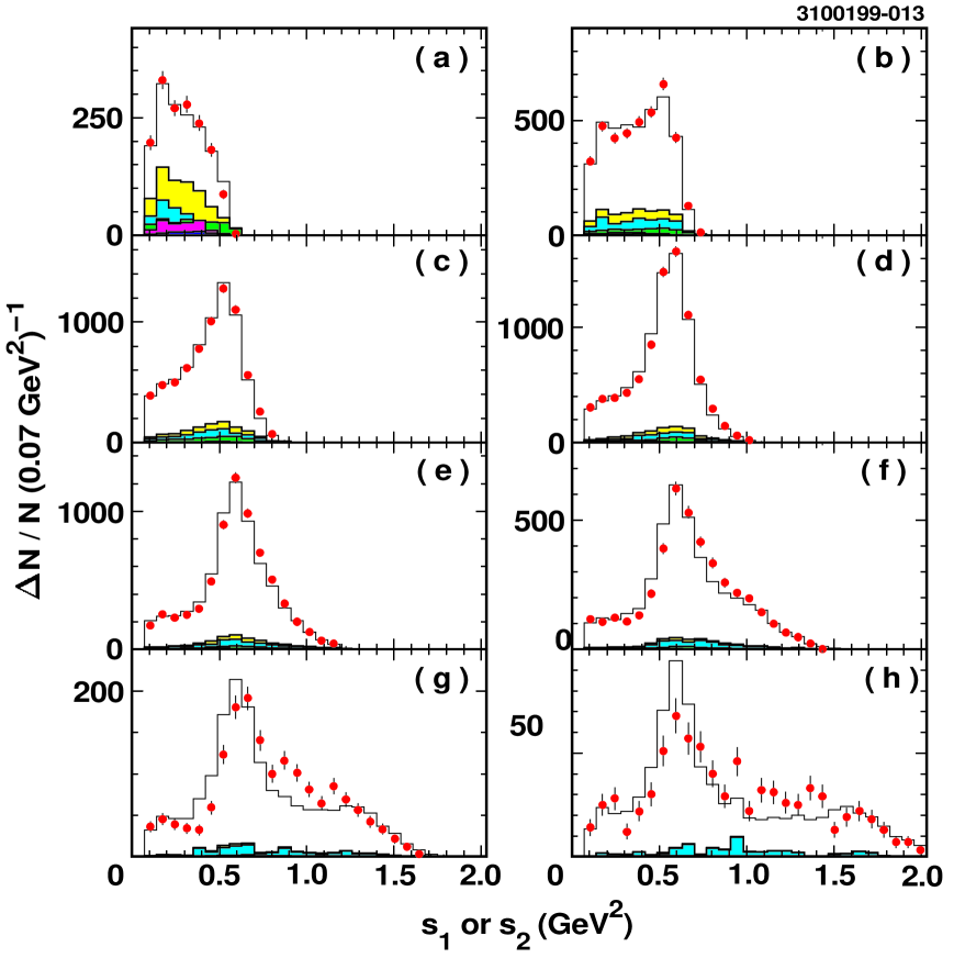
FIG. 11.: Dalitz plot projections: distributions in squared $\pi^{-}\pi^{0}$ mass $s_{1}$ and $s_{2}$ (two entries per event), plotted for slices of $\sqrt{s}$ as in Fig. 3. The data are represented by the filled points. The solid line is the result from a modified version of the nominal fit in which amplitudes involving isoscalar mesons ($\sigma\pi$, $f_{0}\pi$ and $f_{2}\pi$) have been omitted.

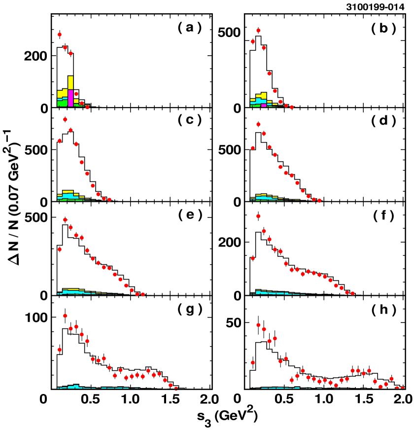
FIG. 12.: Dalitz plot projections: distributions in squared $\pi^{0}\pi^{0}$ mass $s_{3}$ (one entry per event), plotted for slices of $\sqrt{s}$ as in Fig. 4. The data are represented by the filled points. The solid line is the result from a modified version of the nominal fit in which amplitudes involving isoscalar mesons ($\sigma\pi$, $f_{0}\pi$ and $f_{2}\pi$) have been omitted.

C RESULTS FROM FITS WITH FINITE MESON RADII

Treatment of the $a_{1}$ as being point-like results in unphysical behavior of the running width $\Gamma^{a_{1}}_{tot}(s)$ at large values of $s$. The effect of the form factor $F_{R_{i}}(k_{i})$ defined in Eqn. 5 is to damp out this behavior, although the Gaussian form itself is somewhat ad hoc. This form factor affects both the substructure analysis and the $3\pi$ mass spectrum analysis. Although the data at present do not show much sensitivity to the value of the meson size $R$, we note that both analyses prefer values of $R\sim 1.4\,\rm{GeV}^{-1}$. In this appendix we report the results from fits using non-zero values for $R$.

1 Substructure fits

In Table VII, we give the results from the substructure fit with $R_{i}=1.4\,\rm{GeV}^{-1}$. These results are in qualitative agreement with those from the nominal fit.

TABLE VII.: Results from substructure fit with meson radii $R_{i}=1.4\mbox{ GeV}^{-1}$.

		Signif.	$|\beta_{i}|$	$\phi_{\beta_{i}}/\pi$	${\cal B}$ fraction ($\%$)
$\rho$	$s$-wave	–	$1.00$	$0.0$	$69.11$
$\rho(1450)$	$s$-wave	$0.6\sigma$	$0.03\pm 0.06$	$\phantom{-}0.92\pm 0.58$	$0.02\pm 0.08$
$\rho$	$d$-wave	$5.4\sigma$	$0.36\pm 0.09$	$-0.12\pm 0.11$	$0.28\pm 0.13$
$\rho(1450)$	$d$-wave	$3.7\sigma$	$0.78\pm 0.28$	$\phantom{-}0.41\pm 0.14$	$0.28\pm 0.20$
$f_{2}(1270)$	$p$-wave	$4.6\sigma$	$0.66\pm 0.14$	$\phantom{-}0.64\pm 0.10$	$0.11\pm 0.05$
$\sigma$	$p$-wave	$7.9\sigma$	$2.13\pm 0.27$	$\phantom{-}0.27\pm 0.03$	$14.31\pm 3.66$
$f_{0}(1370)$	$p$-wave	$6.1\sigma$	$0.77\pm 0.13$	$-0.47\pm 0.05$	$3.69\pm 1.21$

2 Fits to $M_{3\pi}$

Fits to the $3\pi$ mass spectrum were performed with non-zero values for $R_{i}$ with the assumptions of constant and running $a_{1}$ masses. These studies differed from the nominal fit in Fig. 9 in two additional ways. First, the fitting range included two additional bins in the high mass region, extending up to 1.775 MeV. Second, so as to account for possible systematic effects, the acceptance and background corrections were allowed to vary within reasonable amounts by adding terms to the $\chi^{2}$ constraining their deviations from the nominal assuming these to be Gaussian distributed (see Section VI D).

Results for fits assuming constant and running $a_{1}$ masses are presented in Tables VIII and IX respectively. Similar trends are observed in fits to just the lepton-tagged sample, as well as in fits that include an $a_{1}^{\prime}$ contribution. The final column in the tables, labeled $\sqrt{\chi^{2}_{c}}$, denotes the square root of the contribution of the acceptance and background correction constraints to the total $\chi^{2}$ of the fit. In both constant and running mass scenarios, the $a_{1}$ pole width is strongly affected by the presence of the form factor accounting for the size of the $a_{1}$ meson, and by the value of $R$.

The preferred fits, with $R=1.2\;\mbox{GeV}^{-1}$ for the constant mass case and $R=1.4\;\mbox{GeV}^{-1}$ for the running mass case are plotted in Figures 13(a) and (c), respectively. We have also performed these fits including turn-on of the $f_{0}(980)\pi$ channel, the results of which are plotted in Figures 13(b) and (d) for the two cases.

TABLE VIII.: Results of $3\pi$ mass spectrum fits with different input values of $a_{1}$ size parameter $R$, assuming constant $a_{1}$ mass.

$R$	$\chi^{2}/n_{dof}$	$m_{0a_{1}}$	$\Gamma_{0a_{1}}$	${\cal B}(K^{\star}K)$	$\sqrt{\chi^{2}_{c}}$
$[\mbox{GeV}^{-1}]$		$[\mbox{GeV}]$	$[\mbox{GeV}]$	$[\%]$
$0.0$	40.9/43	$1.330\pm 0.011$	$0.811\pm 0.042$	$3.3\pm 0.6$	$0.32$
$1.0$	38.9/43	$1.289\pm 0.008$	$0.653\pm 0.025$	$3.4\pm 0.6$	$0.32$
$1.2$	38.6/43	$1.285\pm 0.007$	$0.619\pm 0.021$	$3.5\pm 0.6$	$0.31$
$1.3$	39.3/43	$1.279\pm 0.006$	$0.597\pm 0.019$	$3.4\pm 0.7$	$0.33$
$1.4$	39.9/43	$1.274\pm 0.006$	$0.578\pm 0.017$	$3.2\pm 0.7$	$0.37$
$1.5$	42.9/43	$1.269\pm 0.005$	$0.558\pm 0.015$	$3.0\pm 0.7$	$0.38$
$1.6$	45.5/43	$1.263\pm 0.005$	$0.538\pm 0.014$	$2.8\pm 0.7$	$0.44$

TABLE IX.: Results of $3\pi$ mass spectrum fits with different input values of $a_{1}$ size parameter $R$, assuming running $a_{1}$ mass.

$R$	$\chi^{2}/n_{dof}$	$m_{0a_{1}}$	$\Gamma_{0a_{1}}$	${\cal B}(K^{\star}K)$	$\sqrt{\chi^{2}_{c}}$
$[\mbox{GeV}^{-1}]$		$[\mbox{GeV}]$	$[\mbox{GeV}]$	$[\%]$
$1.2$	39.6/43	$1.298\pm 0.007$	$1.200\pm 0.100$	$3.3\pm 0.7$	$0.77$
$1.3$	39.3/43	$1.294\pm 0.006$	$0.822\pm 0.047$	$3.3\pm 0.7$	$0.78$
$1.4$	36.7/43	$1.288\pm 0.006$	$0.667\pm 0.031$	$3.3\pm 0.7$	$0.71$
$1.5$	41.9/43	$1.284\pm 0.006$	$0.558\pm 0.021$	$3.2\pm 0.7$	$0.79$
$1.6$	54.4/43	$1.279\pm 0.005$	$0.493\pm 0.016$	$3.0\pm 0.7$	$0.77$

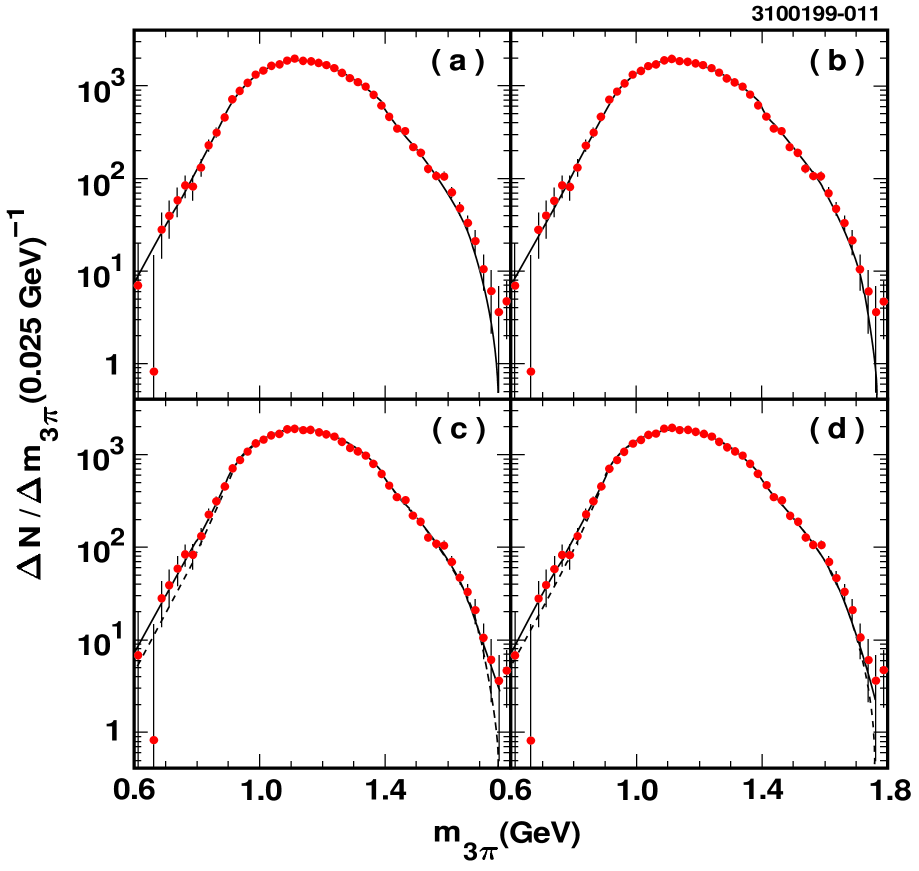
FIG. 13.: Background-subtracted efficiency-corrected $3\pi$ mass spectrum (points with error bars) with fit functions overlaid. The solid curves in plots (a) and (b) represent the fit function with $R=1.2\mbox{ GeV}^{-1}$, assuming a constant mass, excluding (a) and including (b) the effect of the $f_{0}(980)\pi$ threshold on $\Gamma^{a_{1}}_{tot}(s)$. The solid curves in plots (c) and (d) represent the fit function with $R=1.4\mbox{ GeV}^{-1}$, assuming a running mass. The effect of the $f_{0}(980)\pi$ threshold on $\Gamma^{a_{1}}_{tot}(s)$ and $m_{a_{1}}(s)$ is excluded in (c), and included in (d). The dotted curves represent the corresponding fit functions without the deviations in the background subtraction and efficiency correction returned by the fits.

The parametrizations of the $\sqrt{s}$-dependence of the $a_{1}$ mass entering the fits shown in Figs. 13(c) and (d) are plotted in Fig. 14. The overall mass shift function depends on the relative amplitudes for the $K^{*}K$ and (in Fig. 13(d)) $f_{0}(980)\pi$ channels which are fit parameters, however the shapes of the contributions to $m_{a_{1}}(s)$ from these channels are determined as described in Section III B. The effect of successively including thresholds is illustrated by the dotted curve in Fig. 14(a), in which an ad hoc $f_{0}(980)\pi$ contribution is added, assuming unchanged couplings to the other channels. As noted earlier, the effect is to flatten the dependence of $m_{a_{1}}(s)$.

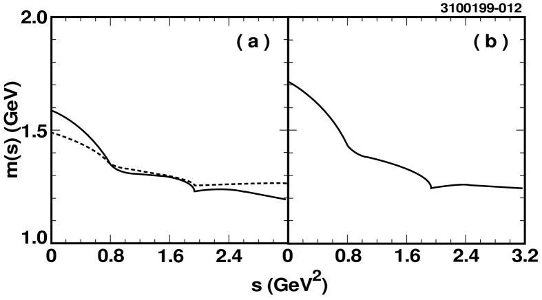
FIG. 14.: The solid curve in plot (a) shows the running mass used in the fit shown in Fig. 13(c). The dotted curve illustrates the effect of adding the $f_{0}(980)\pi$ threshold, with $\Gamma_{3\pi}(s)$ and $\Gamma_{K^{\star}K}$ unchanged. Plot (b) shows the running mass used in the fit shown in Fig. 13(d), where the relative $K^{*}K$ and $f_{0}(980)\pi$ amplitudes are determined from the fit.

Satisfactory fits are obtained with both constant and running $a_{1}$ masses. Functions assuming a running mass yield fits with smaller $\chi^{2}$ values than those with a constant mass. However, the running mass fits also prefer a larger distortion of the background and acceptance corrections, as indicated by the larger values of $\sqrt{\chi^{2}_{c}}$ in Table IX and by the deviations of the dotted curves in Figs. 13(c) and (d) from the corresponding solid curves.

REFERENCES

- [1] Particle Data Group, C. Caso et al., E. Phys. J. C 3, 1 (1998).
- [2] M. G. Bowler, Phys. Lett. 182B, 400 (1986); M. G. Bowler, Phys. Lett. 209B, 99 (1988).
- [3] N. A. Törnqvist, Z. Phys. C 36, 695 (1987); 40, 632(E) (1988).
- [4] N. Isgur, C. Morningstar and C. Reader, Phys. Rev. D 39, 1357 (1989).
- [5] J. H. Kühn and A. Santamaria, Z. Phys. C 48, 445 (1990).
- [6] M. Feindt, Z. Phys. C 48 681 (1990).
- [7] M. K. Volkov, Yu. P. Ivanov and A. A. Osipov, Z. Phys. C 49, 563 (1991).
- [8] H. Albrecht et al., (the ARGUS Collaboration), Z. Phys. C 58, 61 (1993).
- [9] H. Albrecht et al., (the ARGUS Collaboration), Phys. Lett. 349B, 576 (1995); M. Schmidtler, Bestimmung der Michelparameter und in leptonischen -Zerfällen, Dr. thesis, Universität Karlsruhe, IEKP-KA/94-16.
- [10] K. Ackerstaff et al., (the OPAL Collaboration), Z. Phys. C 75, 593 (1997).
- [11] R. McNulty, to appear in proceedings of the Fifth Workshop on Tau Lepton Physics, Santander, Spain, September 1998.
- [12] P. Abreu et al., (the DELPHI Collaboration), Phys. Lett. 426B, 411 (1998).
- [13] L. Passalacqua, Nucl. Phys. B (Proc. Suppl.) 55C 435 (1997), proceedings of the Fourth Workshop on Tau Lepton Physics, Estes Park, Colorado, September 1996.
- [14] R. Barate et al., (the ALEPH Collaboration), E. Phys. J. C 2, 395 (1998).
- [15] T. Bergfeld et al., (the CLEO Collaboration), Phys. Rev. Lett. 79, 2406 (1997).
- [16] Y. Kubota et al., (the CLEO Collaboration), Nucl. Inst. Meth. A320, 66 (1992).
- [17] We use KORALB (v.2.2) / TAUOLA (v.2.4). References for earlier versions are: S. Jadach and Z. Was, Comput. Phys. Commun. 36, 191 (1985); 64, 267 (1991); S. Jadach, J. H. Kühn, and Z. Was, Comput. Phys. Commun. 64, 275 (1991); 70, 69 (1992); 76, 361 (1993).
- [18] R. Brun et al., GEANT 3.15, CERN DD/EE/84-1.
- [19] J. Urheim, Nucl. Phys. B (Proc. Suppl.) 55C, 359 (1997), proceedings of the Fourth Workshop on Tau Lepton Physics, Estes Park Colorado, September 1996.
- [20] N. A. Törnqvist, Z. Phys. C 68, 647 (1995).
- [21] R. Kokoski and N. Isgur, Phys. Rev. D 35, 907 (1987).
- [22] S. Godfrey and N. Isgur, Phys. Rev. D 32, 189 (1985).
- [23] D. V. Amelin et al., (the VES Collaboration), Phys. Lett. 356B, 595 (1995).
- [24] J. P. Alexander et al., (the CLEO Collaboration), Phys. Rev. D 56, 5320 (1997).
- [25] J. H. Kühn and F. Wagner, Nucl. Phys. B236, 16 (1984).
- [26] W. B. Ruckstühl et al., (the DELCO Collaboration), Phys. Rev. Lett. 56, 2132 (1986).
- [27] W. B. Schmidke et al., (the Mark II Collaboration), Phys. Rev. Lett. 57, 527 (1986).
- [28] H. Albrecht et al., (the ARGUS Collaboration), Z. Phys. C 33, 7 (1986).
- [29] J. H. Kühn and E. Mirkes, Z. Phys. C 56 661 (1992); 67 364(E) (1995).