DEMO-HEP 98/04 November 1998

Extended Modified Observable Technique
for a Multi-Parametric Trilinear Gauge Coupling
Estimation at LEP II

G. K. Fanourakis, D. Fassouliotis, A. Leisos,
N. Mastroyiannopoulos and S. E. Tzamarias

Institute of Nuclear Physics - N.C.S.R. Demokritos
15310 - Aghia Paraskevi - Attiki - Greece

This paper describes the extension of the Modified Observables technique in estimating simultaneously more than one Trilinear Gauge Couplings. The optimal properties, unbiasedness and consistent error estimation of this method are demonstrated by Monte Carlo experimentation using $\ell\nu jj$ four-fermion final state topologies. Emphasis is given in the determination of the expected sensitivities in estimating the $\lambda_{\gamma}-\Delta g_{1}^{z}$ and $\Delta k_{\gamma}-\Delta g_{1}^{z}$ pair of couplings with data from the 183 GeV LEPII run.

1 Introduction

It has been shown [1], that by expanding the probability distribution function (p.d.f.) and keeping only linear terms with respect to the Trilinear Gauge Couplings (TGC’s), one can build estimators (the Optimal Observables) which are linear functions of the couplings around the expansion point. Furthermore, this linear dependence can be easily evaluated by theory. An efficient estimation of the couplings can be performed by inverting these linear relations. Such an estimation has the same accuracy as the unbinned maximum likelihood technique.

The method of the Optimal Observables has been extended [2] to incorporate the influence of the detector effects to the measurement of the kinematical vectors. An iterative procedure has been also introduced to ensure the consistency and optimality of the technique, independent of the choice of the parametric expansion point. In the same paper, the optimal properties of this (Modified Observables) method have been demonstrated for one coupling fits to the 172 GeV LEPII data.
In the meanwhile larger data samples are available from the 183 GeV LEPII run and the application of the Modified Observable technique to a simultaneous estimation of two couplings is very relevant.

This paper concentrates on the simultaneous estimation of two TGC’s by employing phenomenological models [3] where two couplings could deviate freely from their Standard Model (S.M.) values whilst certain constraints are imposed on the other couplings. This paper is dealing with WW events produced in $e^{+}e^{-}$ annihilation, where one of the W’s decays leptonically whilst the other decays in two jets. A large sample of 60000 $WW\rightarrow\ell\nu q\bar{q}$ Monte Carlo (M.C.) events was used to evaluate cross sections and other statistics, as well as their dependence on the coupling values by the M.C. reweighting procedure [4]. These events have been produced either by PYTHIA [5] (employing only the CC03 production diagrams) or by EXCALIBUR [6] (full 4-fermion production) at different coupling values and they have undergone full detector simulation by the DELSIM [7] simulation programme. Moreover these events have been reconstructed and selected by the same analysis algorithms as the real data [8] [9] accumulated with the DELPHI [10] detector. The background contamination has been simulated by the production of the physics channels [8] [9] [11] which produce final state topologies indistinguishable from the signal WW events.

This paper is organised as follows: the statistical technique and its asymptotic properties are described in Section 2, whilst numerical results obtained by M.C. experimentation are presented in Section 3. Finally, Section 4 contains the comparison with other techniques and the conclusions.

2 Modified Observables in Multi-Parametric Fits

The present study is focusing on two parameter (TGC’s) estimations but this analysis can be extended to any number of parameters in a straight forward way.

The probability distribution function, with respect to the observed kinematical vector $\vec{\Omega}$, is expressed [2] [3] as a function of the two couplings $\alpha_{1}$ and $\alpha_{2}$ as

$$P(\vec{\Omega};\alpha_{1},\alpha_{2})=\int\frac{d\sigma(\vec{V};\alpha_{1},\alpha_{2})/d\vec{V}}{\sigma_{tot}(\alpha_{1},\alpha_{2})}\cdot\epsilon(\vec{V})\cdot R(\vec{V};\vec{\Omega})\cdot d\vec{V}$$

$$=\int\frac{\sum_{i=0}^{2}\sum_{j=0}^{2-i}c_{ij}(\vec{V})\alpha_{1}^{i}\alpha_{2}^{j}}{\sum_{i=0}^{2}\sum_{j=0}^{2-i}S_{ij}\alpha_{1}^{i}\alpha_{2}^{j}}\cdot\epsilon(\vec{V})\cdot R(\vec{V};\vec{\Omega})\cdot d\vec{V}$$ (1)

where

$\vec{V}$

is the true kinematical vector which describes the events

$\epsilon(\vec{V})$

is the efficiency of observing an event produced at $\vec{V}$

$R(\vec{V};\vec{\Omega})$

is the resolution function, i.e. the probability the true kinematical vector $\vec{V}$ to be measured as $\vec{\Omega}$

$\frac{d\sigma(\vec{V};\alpha_{1},\alpha_{2})}{d\vec{V}}$

is the differential cross-section

$\sigma_{tot}(\alpha_{1},\alpha_{2})$

is the total cross-section and

$S_{ij}=\int c_{ij}(\vec{V})d\vec{V}$.

In [2], it has been shown that the Optimal Observables including detector effects, in the neighbourhood of the parametric point $\{\alpha_{1}^{0},\alpha_{2}^{0}\}$, are defined as the mean values of the following quantities:

$$z_{1}(\vec{\Omega};\alpha_{1}^{0},\alpha_{2}^{0})=\frac{\int y_{01}(\vec{V};\alpha_{1}^{0},\alpha_{2}^{0})\epsilon(\vec{V})R(\vec{V};\vec{\Omega})d\vec{V}}{\int y_{00}(\vec{V};\alpha_{1}^{0},\alpha_{2}^{0})\epsilon(\vec{V})R(\vec{V};\vec{\Omega})d\vec{V}}$$

$$z_{2}(\vec{\Omega};\alpha_{1}^{0},\alpha_{2}^{0})=\frac{\int y_{10}(\vec{V};\alpha_{1}^{0},\alpha_{2}^{0})\epsilon(\vec{V})R(\vec{V};\vec{\Omega})d\vec{V}}{\int y_{00}(\vec{V};\alpha_{1}^{0},\alpha_{2}^{0})\epsilon(\vec{V})R(\vec{V};\vec{\Omega})d\vec{V}}$$ (2)

where the functions $y_{\kappa,\lambda}(\vec{V};\alpha_{1}^{0},\alpha_{2}^{0})$ are expressed in terms of the differential cross section coefficients as:

$$y_{00}(\vec{V};\alpha_{1}^{0},\alpha_{2}^{0}) = c_{00}(\vec{V})+c_{01}(\vec{V})\alpha_{1}^{0}+c_{10}(\vec{V})\alpha_{2}^{0}+c_{20}(\vec{V})\alpha_{1}^{{}_{0}2}+c_{02}(\vec{V})\alpha_{2}^{{}_{0}2}+c_{11}(\vec{V})\alpha_{1}^{0}\alpha_{2}^{0}$$

$$y_{10}(\vec{V};\alpha_{1}^{0},\alpha_{2}^{0}) = c_{10}(\vec{V})+2c_{20}(\vec{V})\alpha_{1}^{0}+c_{11}(\vec{V})\alpha_{2}^{0}$$ (3)

$$y_{01}(\vec{V};\alpha_{1}^{0},\alpha_{2}^{0}) = c_{01}(\vec{V})+2c_{02}(\vec{V})\alpha_{2}^{0}+c_{11}(\vec{V})\alpha_{1}^{0}$$

It has also been shown that the Optimal Observables are linear functions of the couplings $\alpha_{1}$ and $\alpha_{2}$ in the neighbourhood of ($\alpha_{1}^{0},\alpha_{2}^{0}$) i.e.:

$$\int z_{k}(\vec{\Omega};\alpha_{1}^{0},\alpha_{2}^{0})P(\vec{\Omega};\alpha_{1},\alpha_{2})d\vec{\Omega}= \int z_{k}(\vec{\Omega};\alpha_{1}^{0},\alpha_{2}^{0})P(\vec{\Omega};\alpha_{1}^{0},\alpha_{2}^{0})d\vec{\Omega}+$$ (4)

$$\sum_{i=1}^{2}[\int z_{i}(\vec{\Omega};\alpha_{1}^{0},\alpha_{2}^{0})z_{k}(\vec{\Omega};\alpha_{1}^{0},\alpha_{2}^{0})P(\vec{\Omega};\alpha_{1}^{0},\alpha_{2}^{0})d\vec{\Omega}-$$

$$(\int z_{i}(\vec{\Omega};\alpha_{1}^{0},\alpha_{2}^{0})P(\vec{\Omega};\alpha_{1}^{0},\alpha_{2}^{0})d\vec{\Omega}\cdot$$

$$\int z_{k}(\vec{\Omega};\alpha_{1}^{0},\alpha_{2}^{0})P(\vec{\Omega};\alpha_{1}^{0},\alpha_{2}^{0})d\vec{\Omega})]\cdot(\alpha_{i}-\alpha_{i}^{0})$$

where k=1,2

Thus, given a set of N experimentally measured vectors $\vec{\Omega}_{n}$ (n=1,…,N) the left hand side of (4) can be approximated as:

$$\int z_{k}(\vec{\Omega};\alpha_{1}^{0},\alpha_{2}^{0})\vec{P}(\vec{\Omega};\alpha_{1},\alpha_{2})d\vec{\Omega}\simeq\frac{1}{N}\sum_{n=1}^{N}z_{k}(\vec{\Omega}_{n};\alpha_{1}^{0},\alpha_{2}^{0})$$ (5)

The right hand side of (4) can be calculated using the theoretical expression of the cross section as a function of the couplings, provided that the resolution and efficiency functions can be parametrized analytically. Then, a simple inversion of the linear system of equations (4) results to an estimation of the coupling values with the same sensitivity as with the maximum likelihood technique.
In practice, neither the efficiency nor the resolution function can be parametrized analytically. However, it has been shown that a very succesfull approximative way of using the basic concepts of the Optimal Observables in one TGC parameter estimations [2] exists. That is the Modified Observable technique, which in this paper is extended to more than one TGC simultaneous estimations.

Following the same steps as in [2], the functional forms of $z_{1}(\vec{\Omega};\alpha_{1}^{0},\alpha_{2}^{0})$ and $z_{2}(\vec{\Omega};\alpha_{1}^{0},\alpha_{2}^{0})$ in (2) are approximated as:

$$z_{1,2}(\vec{\Omega};\alpha_{1}^{0},\alpha_{2}^{0})\simeq\frac{y_{01,10}(\vec{\Omega};\alpha_{1}^{0},\alpha_{2}^{0})}{y_{00}(\vec{\Omega};\alpha_{1}^{0},\alpha_{2}^{0})}$$ (6)

These are very good approximations, as indicated in figure 1 where the mean values of the quantities $\frac{y_{01,10}(\vec{V};\alpha_{1}^{0},\alpha_{2}^{0})}{y_{00}(\vec{V};\alpha_{1}^{0},\alpha_{2}^{0})}$ are compared with the quantities $\frac{y_{01,10}(\vec{\Omega};\alpha_{1}^{0},\alpha_{2}^{0})}{y_{00}(\vec{\Omega};\alpha_{1}^{0},\alpha_{2}^{0})}$, for several expansion points $\alpha_{1}^{0}$ and $\alpha_{2}^{0}$. These mean values have been evaluated by using M.C. events produced with coupling values $\alpha_{1}^{0}$ and $\alpha_{2}^{0}$ and being observed with kinematical vector $\vec{\Omega}$ corresponding to a bin of $\frac{y_{01,10}(\vec{\Omega};\alpha_{1}^{0},\alpha_{2}^{0})}{y_{00}(\vec{\Omega};\alpha_{1}^{0},\alpha_{2}^{0})}$.
The functional form of $z_{1,2}(\vec{\Omega};\alpha_{1}^{0},\alpha_{2}^{0})$ in (6) is independent of phase space and other multiplicative (e.g. Initial State Radiation) factors and it was calculated by using the ERATO [12] four-fermion matrix element package by folding the kinematical information corresponding to the two hadronic jets.

Instead of calculating the terms of the right hand side of (4), the dependence of the mean values of $z_{1,2}(\vec{\Omega};\alpha_{1}^{0},\alpha_{2}^{0})$ (in the following called Modified Observables ) on the production values of the couplings has been evaluated by reweighted M.C. [4] integration.
Figure 2 shows the surfaces $f_{1}(\alpha_{1},\alpha_{2};\alpha_{1}^{0},\alpha_{2}^{0})$ and $f_{2}(\alpha_{1},\alpha_{2};\alpha_{1}^{0},\alpha_{2}^{0})$ (in the following called calibration surfaces), which express the dependence of the product of each Modified Observable with the number of expected events for luminosity of 50.23 $pb^{-1}$, as a function of the coupling values, for three initial parametric points. These products (instead of the Modified Observables themselves) are going to be used as estimators of the couplings, gaining more efficiency by including the extra information of the total number of the observed events [1].
The couplings are estimated by comparing the calibration surfaces to the experimental measurements, that is to the products of the measured values of the Modified Observables with the number of observed events, which are simply expressed as:

$$d_{1}(\alpha_{1}^{0},\alpha_{2}^{0})=\sum_{i=1}^{N}z_{1}(\vec{\Omega}_{i};\alpha_{1}^{0},\alpha_{2}^{0})$$

$$d_{2}(\alpha_{1}^{0},\alpha_{2}^{0})=\sum_{i=1}^{N}z_{2}(\vec{\Omega}_{i};\alpha_{1}^{0},\alpha_{2}^{0})$$ (7)

Such comparisons are shown in figures (3) and (4) between a large independent set of M.C. events used as a data sample and three pairs of calibration surfaces ($f_{1}(\alpha_{1},\alpha_{2};\alpha_{1}^{0},\alpha_{2}^{0})$ and $f_{2}(\alpha_{1},\alpha_{2};\alpha_{1}^{0},\alpha_{2}^{0})$) evaluated at three different expansion points $\{\alpha_{1}^{0},\alpha_{2}^{0}\}$. In these figures the intersections of the calibration surfaces with the planes defined by the experimental measurements, $d_{1}(\alpha_{1}^{0},\alpha_{2}^{0})$ and $d_{2}(\alpha_{1}^{0},\alpha_{2}^{0})$, are also shown. It is worth noticing that the estimation, which is the common point of the pair of lines in figures 3c, 4c and 4f, is independent from the expansion point. This fact reflects one of the basic properties of the technique to be globally unbiased.
However, the evaluation of the estimation confidence intervals is more complicated, due to the statistical correlations between the calibration surfaces as well as between the measured quantities $d_{1}(\alpha_{1}^{0},\alpha_{2}^{0})$ and $d_{2}(\alpha_{1}^{0},\alpha_{2}^{0})$.
The covariant matrices $M(\alpha_{1},\alpha_{2};\alpha_{1}^{0},\alpha_{2}^{0})$ (expressing the statistical accuracy of the calibration surface evaluation at the expansion point { $(\alpha_{1}^{0},\alpha_{2}^{0})$ } ) and $V(\alpha_{1}^{0},\alpha_{2}^{0})$ (which is the covariant matrix corresponding to the measured quantities $d_{1}(\alpha_{1}^{0},\alpha_{2}^{0})$ and $d_{2}(\alpha_{1}^{0},\alpha_{2}^{0})$) are calculated from the kinematical vectors of the reweighted M.C. and real events respectively.
Then, assuming gaussian errors, the probability that the selected event sample supports coupling values equal to $\alpha_{1}$ and $\alpha_{2}$, is given by the Likelihood function:

$$L=\frac{1}{2\pi\left|W\right|}\cdot exp[-\frac{1}{2}\left(\vec{D}(\alpha_{1}^{0},\alpha_{2}^{0})-\vec{F}(\alpha_{1},\alpha_{2};\alpha_{1}^{0},\alpha_{2}^{0})\right)^{T}\cdot$$

$$W^{-1}\cdot\left(\vec{D}(\alpha_{1}^{0},\alpha_{2}^{0})-\vec{F}(\alpha_{1},\alpha_{2};\alpha_{1}^{0},\alpha_{2}^{0})\right)]$$ (8)

where the vector $\vec{D}(\alpha_{1}^{0},\alpha_{2}^{0})$, the vector calibration function $\vec{F}(\alpha_{1},\alpha_{2};\alpha_{1}^{0},\alpha_{2}^{0})$ and the covariant matrix $W(\alpha_{1},\alpha_{2};\alpha_{1}^{0},\alpha_{2}^{0})$ are defined as follows:

$$\vec{D}(\alpha_{1}^{0},\alpha_{2}^{0})=\left(\begin{array}[]{l}d_{1}(\alpha_{1}^{0},\alpha_{2}^{0})\\ d_{1}(\alpha_{1}^{0},\alpha_{2}^{0})\end{array}\right)$$ (9)

$$\vec{F}(\alpha_{1},\alpha_{2};\alpha_{1}^{0},\alpha_{2}^{0})=\left(\begin{array}[]{l}f_{1}(\alpha_{1},\alpha_{2};\alpha_{1}^{0},\alpha_{2}^{0})\\ f_{2}(\alpha_{1},\alpha_{2};\alpha_{1}^{0},\alpha_{2}^{0})\end{array}\right)$$ (10)

$$W(\alpha_{1},\alpha_{2};\alpha_{1}^{0},\alpha_{2}^{0})=M(\alpha_{1},\alpha_{2};\alpha_{1}^{0},\alpha_{2}^{0})+V(\alpha_{1}^{0},\alpha_{2}^{0})$$ (11)

Maximization of (8), with respect to $\alpha_{1}$ and $\alpha_{2}$, provides the estimation of the coupling values, whilst the confidence intervals are evaluated by the asymptotic gaussian properties of the estimation distribution [13].
A set of M.C. events produced with Standard Model coupling values ( 6000 events at $\{\lambda_{\gamma}=0,\Delta g_{1}^{z}=0\}$), was used as data sample to demonstrate the asymptotic properties of such estimations. The $\lambda_{\gamma},\Delta g_{1}^{z}$ couplings were simultaneously estimated by maximizing the likelihood function of (8) and the estimated coupling values are shown as functions of the expansion point in figure (5). The fact that the estimations are close (within the statistical errors) to the true coupling values, for the whole region of the expansion points, emphasizes the optimal properties of the method. However, the optimal estimated error is achieved [1] at expansion points close to the estimated values, where the linear dependance of the Optimal Variables holds. This is shown in figure 5c where three 70% confidence limit contours corresponding to different expansion points are presented for comparison. Obviously the optimum estimated sensitivity is achieved in the case where $\alpha_{1}^{0}=\hat{\alpha_{1}}$ and $\alpha_{2}^{0}=\hat{\alpha_{2}}$, where $\hat{\alpha_{1}}$ and $\hat{\alpha_{2}}$ are the estimated values. The fact that the above condition also guarantees a correct error estimation, is demonstrated in the next section by Monte Carlo experimentation.

3 Numerical results

A series of M.C. experiments were used to demonstrate the optimal properties of the Modified Observable technique when two TGC’s are simultaneously estimated by fitting finite statistical samples.

Fully reconstructed four fermion EXCALIBUR events, produced with S.M. coupling values, were mixed with background events to form data sets corresponding to the luminosity of 50.23 $pb^{-1}$ accumulated by the DELPHI detector at $\sqrt{s}~{}\simeq~{}183$ GeV. Each set consisted of 82, 101 and 39 events in average with an electron, muon and tau lepton in the final state, respectively. The average background contribution to each of the above subsets were 8.0, 1.4 and 8.3 events. The specific event multiplicity of each data set was chosen to follow poissonian distributions. Another set of fully four fermion and background reconstructed events, produced and selected as described in Section 1, was used to calculate cross sections and probabilties as well as their dependence on the TGC’s by reweighted Monte Carlo integration. In fitting the data sets, the ($\lambda_{\gamma},\Delta g^{Z}_{1}$) and the ($\Delta k_{\gamma},\Delta g^{Z}_{1}$) TGC schemes were used [3] and a simultaneous estimation of the free couplings was performed.
In order to take into account the differences in the production dynamics, the selection efficiencies and the background contamination between the final states ($\ell\nu jj$, $\ell=\mu,e,\tau$) the measured vector $\vec{D}(\alpha_{1}^{0},\alpha_{2}^{0})$ was defined as follows:

$$\vec{D}(\alpha_{1}^{0},\alpha_{2}^{0})=\left(\begin{array}[]{l}\sum_{\ell=1}^{3}(d_{1}^{\ell}(\alpha_{1}^{0},\alpha_{2}^{0})-B_{1}^{\ell})\\ \sum_{\ell=1}^{3}(d_{2}^{\ell}(\alpha_{1}^{0},\alpha_{2}^{0})-B_{2}^{\ell})\end{array}\right)$$ (12)

Where $\ell=1,2,3$ stands for the three lepton tags whilst $B_{1}^{\ell}$, $B_{2}^{\ell}$ denotes the expected contribution of the background events to the measurement.
Similarly the calibration surface vector was defined as:

$$\vec{F}(\alpha_{1},\alpha_{2};\alpha_{1}^{0},\alpha_{2}^{0})=\left(\begin{array}[]{l}\sum_{\ell=1}^{3}f_{1}^{\ell}(\alpha_{1},\alpha_{2};\alpha_{1}^{0},\alpha_{2}^{0})\\ \sum_{\ell=1}^{3}f_{2}^{\ell}(\alpha_{1},\alpha_{2};\alpha_{1}^{0},\alpha_{2}^{0})\end{array}\right)$$ (13)

The asymptotic property of the log likelihood ratio [13] was used to demonstrate the unbiasedness of the proposed techniques. That is, the $\chi^{2}$ (n.d.f.=2) probability of obtaining the specific value of $\lambda$, where

$$\lambda=-2\cdot\log\frac{L(\alpha_{1}^{true},\alpha_{2}^{true})}{L(\hat{\alpha}_{1},\hat{\alpha}_{2})}$$ (14)

in fits of the data sets should follow an equiprobable distribution.
Furthermore, the consistency in evaluating the error matrix of the estimated couplings ($\hat{\cal{E}}$) in every fit, is checked by using the other asymptotic property [13] of the likelihood estimations to be gaussian distributed around the true parameter values. Thus for an unbiased estimation of the central values and for a correct error matrix evaluation the quantity $\delta$:

$$\delta=\left(\begin{array}[]{l}\hat{a_{1}}-a_{1}^{true}\\ \hat{a_{2}}-a_{2}^{true}\end{array}\right)\cdot\hat{\cal{E}}\cdot\left(\begin{array}[]{clcr}\hat{a_{1}}-a_{1}^{true}&\hat{a_{2}}-a_{2}^{true}\end{array}\right)$$ (15)

should follow a $\chi^{2}$(n.d.f.=2) distribution. This property is demonstrated by presenting the $\chi^{2}$(n.d.f.=2) probabilities to obtain specific $\delta$ values in fitting the data sets.
The above tests of $\lambda$ and $\delta$ $\chi^{2}$-probability distributions can be considered as extensions of the sampling and pull distribution tests respectively, commonly used in one parameter fits.

Due to the limited number of the available M.C. events, only sixty independent data sets could be constructed. Although the number of the data sets is enough to show the optimal properties of the proposed technique, the bootstrap procedure [14] has been also used to construct a large number of semicorrelated data sets.

Results of estimating the ($\lambda_{\gamma},\Delta g^{Z}_{1}$) and ($\Delta k_{\gamma},\Delta g^{Z}_{1}$) couplings with the Modified Observable technique are shown in figure 6. In both TGC schemes the optimal properties of the technique in estimating central values and error matrices are obvious. Specifically the sixty completely uncorrelated samples produce $\chi^{2}(n.d.f.=2)$ probabilities distributed with mean values close to 0.5 and root mean squares close to $1/\sqrt{12}$, whilst the equiprobable behaviour of the $\chi^{2}(n.d.f.=2)$ probabililty values obtained by fitting the bootstrapped samples is striking.

The $\chi^{2}$ behaviour of the $\lambda$ and $\delta$ quantities is further used to quantify the sensitivity of this technique. Indeed such property [13] ensures that the estimated values $\{\hat{\alpha_{1}},\hat{\alpha_{2}}\}$ follow a two dimensional gaussian distribution with a covariant matrix which characterises the average sensitivity in estimating the couplings. The covariant matrix elements (i.e. the variances and correlations of the couplings estimations) are found by fitting a 2-dim gaussian to the estimated coupling values from the 60 independent sets. These average sensitivities are summarized in Tables 1 and 2 for ($\lambda_{\gamma},\Delta g^{Z}_{1}$) and ($\Delta k_{\gamma},\Delta g^{Z}_{1}$) estimations.
The same uncorrelated M.C. sets of events were treated as if they have been collected by a “perfect” detector and the two pairs of couplings were estimated by an unbinned extended likelihood fit as well as by the Modified Observable technique . The average sensitivities obtained from these estimations (“perfect” detector extended unbinned likelihood and “perfect” detector Modified Observables) are also shown for comparison in Tables 1 and 2 where the equivalence of the Modified Observables to the likelihood fit is obvious. The loss of sensitivity in the case of a realistic detector is a natural consequence of the loss of information due to the imperfect experimental resolution. However, the consistent inclusion of the detector effects in the realistic case guaranties consistent central value and confidence interval estimation. It is also worth noticing that in the realistic case, the evaluated errors and correlations in every individual Modified Observable estimation are gaussian distributed with means very close to the average sensitivities, as it is shown in figure 7.

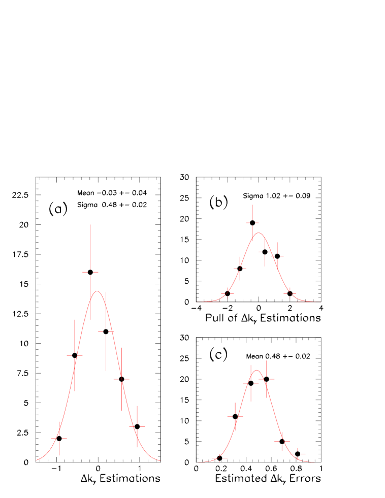
Figure 8: The sampling, pull and error distribution of $\Delta\kappa_{\gamma}$ estimation with the Modified Observable technique.

As a last point, figure 8 shows the sampling, the pull and the error distributions of a single coupling ($\Delta k_{\gamma}$) estimation. Similar estimations of the same coupling [2], using 172 GeV data samples, have been found to exhibit non gaussian tails. However, it was advocated that with small event samples, where the statistical error is large compared to the linear part of the calibration curves, the evaluated error from the fits is expected to underestimate the sensitivity of the technique. Obviously such pathologies are absent when the relative statistical error is smaller, as in the case of the data sample accumulated at 183 GeV.

4 Conclusion

In this paper the Modified Observables technique [2] was generalized in order to be applied for a simultaneous estimation of two couplings by deploying the appropriate TGC scheme [3]. The technique,including the detector effects and the background contribution, was demonstrated to be asymptotically a consistent estimator. This consistency was also shown to be independent of the initial expansion values. However the optimal sensitivity is achieved for expansion points close to the estimated values of the couplings.
The properties of the technique, when fitting finite size event samples, were investigated by M.C. experimentation. Sets of M.C. events, of the same size as the data samples accumulated by each of the LEP experiments at $\sqrt{s}~{}\simeq~{}183$ GeV, were fitted to estimate the $\{\lambda_{\gamma},\Delta g_{1}^{z}\}$ and $\{\Delta\kappa_{\gamma},\Delta g_{1}^{z}\}$ pairs of couplings. The distributions of these estimations demostrated the optimal behaviour (unbiasedness, consistent error matrix evaluation) of the technique. Moreover a comparison with the unbinned extended likelihood results shows that the Modified Observable estimators are practically reaching the maximum sensitivity. These two methods are completely equivalent at the “perfect” detector case (tables 1 and 2). A deterioration of the sensitivity (up to 20%) when dealing with realistic detectors is due to the imperfect resolution of the measuring apparatus.
A comparison [9] between the sensitivity of several multiparametric TGC estimators, which include detector effects, shows that the Modified Observables are equivalent to the Iterative Optimal Variables and Multidimensional Clustering techniques [15] whilst outperform classical methods of one or two dimensional binned likelihood fits.

Method	$\lambda_{\gamma}$ - $\Delta g_{1}^{z}$
	$\sigma_{\lambda_{\gamma}}$	$\sigma_{\Delta g_{1}^{z}}$	$\rho$
“Perfect” Extended Likelihood	0.21 $\pm$ 0.01	0.20 $\pm$ 0.01	-0.73 $\pm$ 0.06
“Perfect” Modified Observables	0.22 $\pm$ 0.01	0.21 $\pm$ 0.01	-0.74 $\pm$ 0.06
Modified Observables	0.25 $\pm$ 0.01	0.23 $\pm$ 0.01	-0.74 $\pm$ 0.06

Table 1: Comparison of the statistical properties of the technique proposed in this paper with the unbinned extended likelihood estimations.

Method	$\Delta k_{\gamma}$ - $\Delta g_{1}^{z}$
	$\sigma_{\Delta k_{\gamma}}$	$\sigma_{\Delta g_{1}^{z}}$	$\rho$
“Perfect” Extended Likelihood	0.35 $\pm$ 0.03	0.14 $\pm$ 0.01	-0.22 $\pm$ 0.08
“Perfect” Modified Observables	0.38 $\pm$ 0.03	0.13 $\pm$ 0.01	-0.25 $\pm$ 0.09
Modified Observables	0.44 $\pm$ 0.03	0.15 $\pm$ 0.01	-0.28 $\pm$ 0.10

Table 2: Comparison of the statistical properties of the techniques proposed in this paper with the unbinned extended likelihood estimations.

Figure 1: The mean values (see text) of the quantities $\frac{y_{10}(\vec{V};\alpha_{1}^{0},\alpha_{2}^{0})}{y_{00}(\vec{V};\alpha_{1}^{0},\alpha_{2}^{0})}$ [(a),(c),(e)] and $\frac{y_{01}(\vec{V};\alpha_{1}^{0},\alpha_{2}^{0})}{y_{00}(\vec{V};\alpha_{1}^{0},\alpha_{2}^{0})}$ [(b),(d),(f)] as functions of the $\frac{y_{10}(\vec{\Omega};\alpha_{1}^{0},\alpha_{2}^{0})}{y_{00}(\vec{\Omega};\alpha_{1}^{0},\alpha_{2}^{0})}$ and $\frac{y_{01}(\vec{\Omega};\alpha_{1}^{0},\alpha_{2}^{0})}{y_{00}(\vec{\Omega};\alpha_{1}^{0},\alpha_{2}^{0})}$ respectively. These mean values correspond to kinematical vectors produced with couplings:

$\alpha_{1}(\equiv\Delta g_{1}^{z})=0$, $\alpha_{2}(\equiv\lambda_{\gamma})=0$ in (a) and (b)
$\alpha_{1}(\equiv\Delta g_{1}^{z})=0$, $\alpha_{2}(\equiv\lambda_{\gamma})=-1$ in (c) and (d)
$\alpha_{1}(\equiv\Delta g_{1}^{z})=0$, $\alpha_{2}(\equiv\lambda_{\gamma})=+1$ in (e) and (f)

Figure 2: The $f_{1}(\alpha_{1},\alpha_{2};\alpha_{1}^{0},\alpha_{2}^{0})$, $f_{2}(\alpha_{1},\alpha_{2};\alpha_{1}^{0},\alpha_{2}^{0})$ calibration surfaces for several expansion points $\alpha_{1}^{0}(\equiv\Delta g_{1}^{z})=0$ , $\alpha_{2}^{0}(\equiv\lambda_{\gamma})=0$ in (a) and (b), $\alpha_{1}^{0}(\equiv\Delta g_{1}^{z})=0$, $\alpha_{2}^{0}(\equiv\lambda_{\gamma})=+1$ in (c) and (d), $\alpha_{1}^{0}(\equiv\Delta g_{1}^{z})=0$, $\alpha_{2}^{0}(\equiv\lambda_{\gamma})=-1$ in (e) and (f).

Figure 3: The calibration surfaces $f_{1}(\alpha_{1},\alpha_{2};\alpha_{1}^{0},\alpha_{2}^{0})$, $f_{2}(\alpha_{1},\alpha_{2};\alpha_{1}^{0},\alpha_{2}^{0})$ as functions of the couplings $\alpha_{1}=\Delta g_{1}^{z}$, $\alpha_{2}=\lambda_{\gamma}$ at the expansion point {$\alpha_{1}^{0}=0$, $\alpha_{2}^{0}=0$}. The horizontal shadowed planes correspond to the experimental measurements. The two lines representing the intersection of the calibration surfaces with the measured values are shown in (c).

Figure 4: The calibration surfaces $f_{1}(\alpha_{1},\alpha_{2};\alpha_{1}^{0},\alpha_{2}^{0})$, $f_{2}(\alpha_{1},\alpha_{2};\alpha_{1}^{0},\alpha_{2}^{0})$ as functions of the couplings $\alpha_{1}=\Delta g_{1}^{z}$, $\alpha_{2}=\lambda_{\gamma}$ at the expansion points {$\alpha_{1}^{0}=0$, $\alpha_{2}^{0}=-1$} in [(a),(b)] and {$\alpha_{1}^{0}=0$, $\alpha_{2}^{0}=+1$} in [(d),(e)]. The horizontal shadowed planes correspond to the experimental measurements. The two lines representing the intersection of the calibration surfaces with the measured values are shown in (c) and (f) for the two pairs of expansion points, respectively.

Figure 5: In [(a) and (b)] the estimated $\alpha_{1}=\Delta g_{1}^{z}$ and $\alpha_{2}=\lambda_{\gamma}$ coupling values as functions of the expansion points are shown. In (c) the evaluated 70% C.L. contours for $\alpha_{1}^{0}=0,\alpha_{2}^{0}=0$ (solid points), $\alpha_{1}^{0}=0.2,\alpha_{2}^{0}=-0.6$ (squares) and $\alpha_{1}^{0}=-0.2,\alpha_{2}^{0}=0.6$ (stars) are compared.

Figure 6: The distributions of $\chi^{2}$ (n.d.f.=2) probabilities in obtaining $\lambda$ [(a),(b),(e),(f)] and $\delta$ [(c),(d),(g),(h)] values in $\{\lambda_{\gamma}$,$\Delta g_{1}^{z}\}$ [(a),(b),(c),(d)] and $\{\Delta\kappa_{\gamma}$,$\Delta g_{1}^{z}\}$ [(e),(f),(g),(h)] estimations by the Modified Observables technique. The lines with slopes consistent with zero in (b),(d),(f) and (h) are first degree polynomial fits to the bootstrap results.

Figure 7: Confidence interval estimations with the Modified Observables technique. The distributions of errors [(a),(b),(d),(e)] and correlations [(c),(f)] in estimating the $\{\lambda_{\gamma},\Delta g_{1}^{z}\}$ [(a),(b),(c)] and $\{\Delta\kappa_{\gamma},\Delta g_{1}^{z}\}$ [(d),(e),(f)] pair of couplings. The data points correspond to the 60 independent data sets whilst the histograms to the bootstrap results. The arrows indicate the average sensitivities summarized in Tables 1 and Table 2.

References

• [1] M. Diehl and O. Nachtmann, Z. Phys. C62 (1994) 397
C.G. Papadopoulos Phys. Let. B386 (1996) 442
M. Diehl and O. Nachtman, HD-THEP-97-03,CPTH-S494-0197,hep-ph/9702208 (1997)
• [2] G.K. Fanourakis, D.A. Fassouliotis and S.E. Tzamarias, Accurate Estimation of the Trilinear Gauge Couplings using Optimal Observables including Detector effects, HEP-EX/9711015 (to appear in NIM A (1998))
• [3] G. Gounaris, J.-L. Kneur and D. Zeppenfeld, in Physics at LEP2, eds G. Altarelli, T. Sjostrand and F. Zwinger, CERN 96-01 Vol. 1,525(1996)
• [4] G.K. Fanourakis, D.A. Fassouliotis and S.E. Tzamarias, A method to include detector effects in estimators sensitive to the Trilinear Gauge Couplings, HEP-EX/9711014 (to appear in NIM A (1998))
• [5] T. Sjöstrand, PYTHIA 5.6 and JETSET 7.3, CERN-TH/6488-92.
• [6] F.A. Berends, R. Kleis and R. Pittau, EXCALIBUR, Physics at LEP2, eds G. Altarelli, G. T. Sjostrand and F. Zwinger, CERN 96-01 Vol. 2, 23(1996)
• [7] DELSIM Reference Manual, DELPHI note, DELPHI 87-97 PROG-100
• [8] T.J.V Bowcock et al, Measurement of Trilinear Gauge Boson Couplings WWV in e+e- Collisions at 183 GeV, DELPHI 98-94 CONF 162
• [9] G. K. Fanourakis et al Comparison of Trilinear Gauge Couplings Estimation Techniques DELPHI 98-154 PHYS 797.
• [10] DELPHI Collaboration: P. Abreu et al., Nucl. Instr. & Meth. A303 (1991) 233
DELPHI Collaboration: P. Abreu et al., Nucl. Instr. & Meth. A378 (1996) 57
• [11] P. Abreu et al., Phys.Lett. B423 (1998) 194
P. Abreu et al., E.Phys.J. C2(1998) 581
• [12] ERATO: event generator for four-fermion production at LEP II energies and beyond C. G. Papadopoulos, Comp. Phys. Comm. 101, (1997) 183.
The part of the ERATO code which calculates the coefficients of the polynomial representation of the matrix elements was extracted and used as a stand alone package.
• [13] See for example Statistical Methods in Experimental Physics, W.T. Eadie et al, North-Holland P.C. (1988).
• [14] See for example
B. Efron, Better bootstrap confidence intervals, Journal of the American Statistical Association, Vol 82, No. 397, (1987), 171-185.
An Introduction to the Bootstrap (Monographs on Statistics and Applied Probability, No 57) by Bradley Efron and Robert J. Tibshirani, Published by Chapman & Hall
• [15] G. Fanourakis et al. Multidimensional Binning Techniques for a Two Parameter Trilinear Gauge Coupling Estimation at LEPII DELPHI 98-148 PHYS 792