DEMO-HEP 98/03 November 1998

Multidimensional Binning Techniques
for a Two Parameter Trilinear Gauge Coupling
Estimation at LEP II

G. K. Fanourakis, D. Fassouliotis, A. Leisos,
N. Mastroyiannopoulos and S. E. Tzamarias

Institute of Nuclear Physics - N.C.S.R. Demokritos
15310 - Aghia Paraskevi - Attiki - Greece

This paper describes two generalization schemes of the Optimal Variables technique in estimating simultaneously two Trilinear Gauge Couplings. The first is an iterative procedure to perform a 2-dimensional fit using the linear terms of the expansion of the probability density function with respect to the corresponding couplings, whilst the second is a clustering method of probability distribution representation in five dimensions. The pair production of W’s at 183 GeV center of mass energy, where one W decays leptonically and the other hadronically, was used to demonstrate the optimal properties of the proposed estimation techniques.

1 Introduction

The precision in measuring physical parameters is strongly dependent on the incorporation of the detector resolution and efficiency into the statistical estimators. However when several kinematical variables are needed to describe the physics process, the convolution of the theoretical predictions with the detector effects is a difficult task. This is the case of the Trilinear Gauge Couplings (TGC’s) estimation at LEPII from the pair production of W bosons, where one deals with an 8-dimensional phase space. In this case, the resolution function describing the measuring process is an 8x8 matrix with elements functions of the kinematical vector. There is no practical way to parameterize analytically such detector dependence unless an enormous amount of Monte Carlo (M.C.) events is available. An alternative procedure would be to project the probability distribution function to a subset of kinematical variables, thus decreasing the order of the resolution matrix, without losing in sensitivity.

In a previous paper [1] it has been shown that, in one TGC estimation, the probability distribution function (p.d.f.) $P(\vec{V};\alpha)$ can be projected on the two variables $x_{1}$ and $x_{2}$ (the Optimal Variables) without any loss of information. Specifically, in a phenomenological scheme where only one coupling is free to deviate from the Standard Model value [2], the differential cross section with respect to the 8-dimensional kinematical vector $\vec{V}$ has a quadratic dependence on the free coupling $\alpha$ of the form:

$$\frac{d\sigma}{d\vec{V}}=c_{0}(\vec{V})+c_{1}(\vec{V})\cdot\alpha+c_{2}(\vec{V})\cdot\alpha^{2}$$ (1)

The p.d.f. $P(\vec{V};\alpha)$, which carries the whole information concerning the coupling $\alpha$, is then defined as:

$$P(\vec{V};\alpha)\cdot d\vec{V}=\frac{(c_{0}(\vec{V})+c_{1}(\vec{V})\cdot\alpha+c_{2}(\vec{V})\cdot\alpha^{2})}{(S_{0}+S_{1}\cdot\alpha+S_{2}\cdot\alpha^{2})}\cdot d\vec{V}$$ (2)

where the denominator is the total cross section, i.e. :

$$S_{i}\equiv\int c_{i}(\vec{V})\cdot d\vec{V}$$ (3)

The projection of (2), on a plane defined by the two Optimal Variables $x_{1}$ and $x_{2}$,

$$\varpi(x_{1},x_{2};\alpha)=\int P(\vec{V};\alpha)\cdot\delta(x_{1}-\frac{c_{1}(\vec{V})}{c_{0}(\vec{V})})\cdot\delta(x_{2}-\frac{c_{2}(\vec{V})}{c_{0}(\vec{V})})\cdot d\vec{V}$$ (4)

contains all the information. The functional form of the Optimal Variables ( $x_{1}=\frac{c_{1}(\vec{V})}{c_{0}(\vec{V})}$, $x_{2}=\frac{c_{2}(\vec{V})}{c_{0}(\vec{V})}$) is independent of phase space or other multiplicative (e.g. Initial State Radiation) factors, containing only the coefficients of the polynomial realization of the squared Matrix element by folding the kinematical information corresponding to the hadronic jets.
When detector effects are to be taken into account, the Optimal Variables are defined by the convolution of the differential cross section with the resolution and efficiency functions. However, it has been shown [1] that their functional form can be approximated very precisely as:

$$x_{1}\cong\frac{c_{1}(\vec{\Omega})}{c_{0}(\vec{\Omega})},x_{2}\cong\frac{c_{2}(\vec{\Omega})}{c_{0}(\vec{\Omega})}$$ (5)

where $\vec{\Omega}$ is the measured kinematical vector.

A binned likelihood fit, in bins of $x_{1}$,$x_{2}$, was demonstrated to estimate the coupling with maximal accuracy even in cases of small statistical ( 172 LEPII Run [1],[4]) samples.

Despite the success of the Optimal Variable method in one parameter estimation, the same technique is not easily extended to multi parametric fits. As an example, in a TGC scheme where two couplings can deviate from their S.M. values, the p.d.f. is written as:

$$P(\vec{V};\alpha_{1},\alpha_{2})\cdot d\vec{V}=\frac{\sum_{i=0}^{2}\sum_{j=0}^{2-i}c_{ij}(\vec{V})\cdot\alpha_{1}^{i}\cdot\alpha_{2}^{j}}{\sum_{i=0}^{2}\sum_{j=0}^{2-i}S_{ij}\alpha_{1}^{i}\alpha_{2}^{j}}\cdot d\vec{V}$$ (6)

In this scheme five Optimal Variables are needed to contain the whole information, namely:

$$x_{1}=\frac{c_{01}(\vec{V})}{c_{00}(\vec{V})},x_{2}=\frac{c_{10}(\vec{V})}{c_{00}(\vec{V})}$$

$$x_{3}=\frac{c_{20}(\vec{V})}{c_{00}(\vec{V})}$$ (7)

$$x_{4}=\frac{c_{02}(\vec{V})}{c_{00}(\vec{V})},x_{5}=\frac{c_{11}(\vec{V})}{c_{00}(\vec{V})}$$

Although there are other maximum likelihood equivalent strategies [1], [3], [5] which are reducing further the number of the necessary variables, it is interesting to see that unbiased and efficient binned likelihood fits can be made in many dimensions, as well.

In this paper we propose two new techniques of performing two TGC simultaneous estimations based on evaluating the cross section of the process $e^{+}e^{-}\rightarrow\ell\nu jj$ in bins of the Optimal Variables. In both methods the M.C. reweighting procedure is used [6] to express the cross sections and the probabilities in every bin as functions of the two TGC couplings. The reweighted sample of M.C. events consisted of 60000 fully reconstructed four fermion events in $\ell\nu jj$ final states. A fraction about the 40% of them have been generated by PYTHIA [8] (including only CCO3 production processes), another 40% are generated by EXCALIBUR [9](including the full list of 4 fermion diagrams) at Standard Model (S.M.) coupling values. The remaining 20% of theses events are generated by EXCALIBUR at several anomalous coupling values.
The simulation of the detector effects was performed by deploying the DELSIM [10] package whilst the event selection algorithms were the same as the ones described in [11] and [12]. The effect of the background contamination to the data samples has been studied by producing M.C. sets corresponding to physical processes [2],[4], [11] with final state topologies accepted by the selection criteria of the genuine WW events.

2 Iterative estimation with Optimal Variables

The p.d.f. (6) can be written in a Taylor expansion around the parametric point $\{\alpha_{1}^{0},\alpha_{2}^{0}\}$ as:

$$P(\vec{V};\alpha_{1},\alpha_{2})=\frac{y_{00}(\vec{V})}{\Sigma_{00}}\cdot[1+(\frac{y_{10}(\vec{V})}{y_{00}(\vec{V})}-\frac{\Sigma_{10}}{\Sigma_{00}})\cdot\delta_{\alpha_{1}}+(\frac{y_{01}(\vec{V})}{y_{00}(\vec{V})}-\frac{\Sigma_{20}}{\Sigma_{00}})\cdot\delta_{\alpha_{2}}]+O(\delta_{\alpha_{1}}^{2},\delta_{\alpha_{2}}^{2})$$ (8)

where:

$$y_{00}(\vec{V};\alpha_{1}^{0},\alpha_{2}^{0}) = c_{00}(\vec{V})+c_{01}(\vec{V})\alpha_{1}^{0}+c_{10}(\vec{V})\alpha_{2}^{0}+c_{20}(\vec{V})\alpha_{1}^{{}_{0}2}+c_{02}(\vec{V})\alpha_{2}^{{}_{0}2}+c_{11}(\vec{V})\alpha_{1}^{0}\alpha_{2}^{0}$$

$$y_{10}(\vec{V};\alpha_{1}^{0},\alpha_{2}^{0}) = c_{10}(\vec{V})+2c_{20}(\vec{V})\alpha_{1}^{0}+c_{11}(\vec{V})\alpha_{2}^{0}$$

$$y_{01}(\vec{V};\alpha_{1}^{0},\alpha_{2}^{0}) = c_{01}(\vec{V})+2c_{02}(\vec{V})\alpha_{2}^{0}+c_{11}(\vec{V})\alpha_{1}^{0}$$ (9)

$$\Sigma_{ij} = \int y_{ij}(\vec{V})d\vec{V}$$

and $\delta_{\alpha_{1}}$, $\delta_{\alpha_{2}}$ being the deviations from $\alpha_{1}^{0}$ and $\alpha_{2}^{0}$ respectively. For coupling values close to the expansion point, the p.d.f. is accurately approximated by keeping only the linear terms of (8). In this approximation the p.d.f. is a function of the variables

$$z_{1}(\vec{V};\alpha_{1}^{0},\alpha_{2}^{0}) = \frac{y_{10}(\vec{V};\alpha_{1}^{0},\alpha_{2}^{0})}{y_{00}(\vec{V};\alpha_{1}^{0},\alpha_{2}^{0})}$$ (10)

$$z_{2}(\vec{V};\alpha_{1}^{0},\alpha_{2}^{0}) = \frac{y_{01}(\vec{V};\alpha_{1}^{0},\alpha_{2}^{0})}{y_{00}(\vec{V};\alpha_{1}^{0},\alpha_{2}^{0})}$$

rather than the kinematical vector $\vec{V}$ itself.

By including the influence of the detector in the determination of the kinematical variables, the p.d.f. with respect to the measured kinematical vector $\vec{\Omega}$ should be expressed as:

$$P(\vec{\Omega};\alpha_{1},\alpha_{2})\cdot d\vec{\Omega}=\int\frac{\sum\sum c_{ij}(\vec{V})\cdot\alpha_{1}^{i}\cdot\alpha_{2}^{j}}{\sum\sum S_{ij}\cdot\alpha_{1}^{i}\cdot\alpha_{2}^{j}}\cdot\epsilon(\vec{V})\cdot R(\vec{V};\vec{\Omega})d\vec{V}d\vec{\Omega}$$ (11)

where $\epsilon(\vec{V})$ is the differential efficiency, and $R(\vec{V};\vec{\Omega})$ is the resolution function. By expanding (11) in a Taylor series around the $\{\alpha_{1}^{0},\alpha_{2}^{0}\}$ parametric point, a similar expression as in (8) is achieved. Namely:

$$P(\vec{\Omega};\alpha_{1},\alpha_{2})=\frac{y_{00}^{{}^{\prime}}(\vec{\Omega};\alpha_{1}^{0},\alpha_{2}^{0})}{\Sigma_{00}}\cdot[1+(\frac{y_{10}^{{}^{\prime}}(\vec{\Omega};\alpha_{1}^{0},\alpha_{2}^{0})}{y_{00}^{{}^{\prime}}(\vec{\Omega};\alpha_{1}^{0},\alpha_{2}^{0})}-\frac{\Sigma_{10}}{S_{00}})\cdot\delta_{\alpha_{1}}+(\frac{y_{01}^{{}^{\prime}}(\vec{\Omega};\alpha_{1}^{0},\alpha_{2}^{0})}{y_{00}^{{}^{\prime}}(\vec{\Omega};\alpha_{1}^{0},\alpha_{2}^{0})}-\frac{\Sigma_{20}}{\Sigma_{00}})\cdot\delta_{\alpha_{2}}]+O(\delta_{\alpha_{1}}^{2},\delta_{\alpha_{2}}^{2})$$ (12)

where the terms $y_{ij}^{{}^{\prime}}(\vec{\Omega};\alpha_{1}^{0},\alpha_{2}^{0})$ are convolutions of the functions $y_{ij}(\vec{V};\alpha_{1}^{0},\alpha_{2}^{0})$, given in (9), with the detector functions i.e.

$$y_{ij}^{{}^{\prime}}(\vec{\Omega})=\int y_{ij}(\vec{V};\alpha_{1}^{0},\alpha_{2}^{0})\epsilon(\vec{V})R(\vec{V},\vec{\Omega})d\vec{V}$$ (13)

The Optimal Variables, ignoring higher orders in (12), are the ratios:

$$z_{1}^{{}^{\prime}}(\alpha_{1}^{0},\alpha_{2}^{0}) = \frac{\int y_{10}(\vec{V};\alpha_{1}^{0},\alpha_{2}^{0})\epsilon(\vec{V})R(\vec{V},\vec{\Omega})d\vec{V}}{\int y_{00}(\vec{V};\alpha_{1}^{0},\alpha_{2}^{0})\epsilon(\vec{V})R(\vec{V},\vec{\Omega})d\vec{V}}$$ (14)

$$z_{2}^{{}^{\prime}}(\alpha_{1}^{0},\alpha_{2}^{0}) = \frac{\int y_{01}(\vec{V};\alpha_{1}^{0},\alpha_{2}^{0})\epsilon(\vec{V})R(\vec{V},\vec{\Omega})d\vec{V}}{\int y_{00}(\vec{V};\alpha_{1}^{0},\alpha_{2}^{0})\epsilon(\vec{V})R(\vec{V},\vec{\Omega})d\vec{V}}$$

As it has been shown in [5] the functional form of the Optimal Variables, including detector effects, can be approximated as:

$$z_{1}^{{}^{\prime}}(\vec{\Omega};\alpha_{1}^{0},\alpha_{2}^{0}) \simeq \frac{y_{10}(\vec{\Omega};\alpha_{1}^{0},\alpha_{2}^{0})}{y_{00}(\vec{\Omega};\alpha_{1}^{0},\alpha_{2}^{0})}$$ (15)

$$z_{2}^{{}^{\prime}}(\vec{\Omega};\alpha_{1}^{0},\alpha_{2}^{0}) \simeq \frac{y_{01}(\vec{\Omega};\alpha_{1}^{0},\alpha_{2}^{0})}{y_{00}(\vec{\Omega};\alpha_{1}^{0},\alpha_{2}^{0})}$$

where the measured kinematical vector $\vec{\Omega}$, instead of the real vector $\vec{V}$, is used to define the expansion coefficients in eq(9).

Based on this analysis, the simultaneous estimation of two couplings is realized by an iterative procedure consisted of the following steps:

1. Define the functional form of the Optimal Variables around the expansion point $\{\alpha_{1}^{0},\alpha_{2}^{0}\}$, as in (10) and (15), by using the observed kinematical vectors as input to the ERATO [7] four-fermion matrix element package.

2. Evaluate the differential cross sections ($\Delta_{i}(\alpha_{1},\alpha_{2})$ $i=1,2,\ldots,k$) in k 2-dimensional bins of the Optimal Variables as functions of the $\alpha_{1}$ and $\alpha_{2}$ TGC values by means of a reweighted Monte Carlo integration.

3. Estimate the couplings values by maximizing an extended likelihood function, thus taking into account the total number of the observed events. In order to include inaccuracies due to the M.C. evaluation of the cross sections, the extended likelihood function is written as:

   $$L^{E}(\alpha_{1},\alpha_{2};\alpha_{1}^{0},\alpha_{2}^{0})=\prod_{i=1}^{k}\int\frac{\mu_{i}^{n_{i}}e^{-\mu_{i}}}{n_{i}!}\frac{e^{-\frac{(\mu_{i}-\delta_{i}(\alpha_{1},\alpha_{2}))^{2}}{2\sigma_{i}^{2}(\alpha_{1},\alpha_{2})}}}{\sqrt{2\pi}\sigma_{i}(\alpha_{1},\alpha_{2})}d\mu_{i}$$ (16)

   where

   $\delta_{i}(\alpha_{1},\alpha_{2})=\Delta_{i}(\alpha_{1},\alpha_{2})\cdot{\cal{L}}$ is the number of the expected events in the bin i for coupling values $\alpha_{1}$ and $\alpha_{2}$ and integrated luminosity ${\cal{L}}$.

   $\sigma_{i}(\alpha_{1},\alpha_{2})$ is the estimated error in the determination of $\delta_{i}(\alpha_{1},\alpha_{2})$

   $n_{i}$ is the number of the observed events in the bin i.

4. The likelihood estimations of the couplings, $\hat{\alpha_{1}}$ and $\hat{\alpha_{2}}$, are used as a new expansion point at the step 1 and the whole procedure is repeated.
   The iteration method is considered to converge when the estimated values of the couplings are equal to those which have been used as expansion values.

The converging properties of the proposed technique are demonstrated by a simultaneous estimation of the $\Delta g_{1}^{z}$ and $\lambda_{\gamma}$ couplings using M.C. generated events as data samples. These are three sets of M.C. events produced by the EXCALIBUR four fermion generator at different points of the parametric space undergone full detector simulation, and have been reconstructed and selected in the same way as the real data [11]. In figures 1a and 1c the deviations of the two couplings estimated values ($\hat{\alpha}_{1}=\hat{\lambda}_{\gamma}$,$\hat{\alpha}_{2}=\Delta\hat{g}_{1}^{z}$) from the corresponding expansion values (${\alpha}_{1}^{0}=\lambda_{\gamma}^{0},{\alpha}_{2}^{0}=\Delta g_{1}^{z^{0}}$) are shown, for several expansion points. These are the estimated couplings by applying the proposed technique to the M.C. set of events which has been produced with S.M. values. The intersections of these deviation surfaces with the plane of zero deviation, corresponding to the fits where the estimated values of each individual coupling are equal to the expansion point, are shown in figure 1b and 1d. The geometry of these intersection lines is such that there is only one parametric point at which the expansion and estimated values are equal for both couplings. This point of convergence (indicated on both the intersections as a star) is very close to the S.M. couplings used for the generation of the data samples. In figure 2, similar deviation surfaces are shown, corresponding to the sets produced with $\lambda_{\gamma}=1$, $\Delta g_{1}^{z}=0$ (a,b,c,d) and $\lambda_{\gamma}=-1$, $\Delta g_{1}^{z}=0$ (e,f,g,h) values. The convergence points in these last examples are also consistently matching the true coupling values.

3 Multidimensional fits with the Clustering technique

The general expression of the p.d.f. (11) depends on the measured kinematical vector $\vec{\Omega}$ through the five Optimal Variables:

$$\omega_{ij}(\vec{\Omega})=\frac{\int c_{ij}(\vec{V})\cdot\epsilon(\vec{V})R(\vec{V};\vec{\Omega})d\vec{V}}{\int c_{00}(\vec{V})\cdot\epsilon(\vec{V})R(\vec{V};\vec{\Omega})d\vec{V}}$$ (17)

That is the projection

$$\Pi(R_{1},R_{2},\ldots,R_{5};\alpha_{1},\alpha_{2})=\int P(\vec{\Omega};\alpha_{1},\alpha_{2})\delta(R_{1}-\omega_{01})\cdot\delta(R_{2}-\omega_{10})\cdot\ldots\cdot\delta(R_{5}-\omega_{11})\cdot d\vec{\Omega}$$ (18)

carries the whole information concerning the couplings $\alpha_{1}$ and $\alpha_{2}$. Furthermore by writing (17) as :

$$\omega_{ij}(\vec{\Omega})=\int\frac{c_{ij}(\vec{V})}{c_{00}(\vec{V})}\cdot\frac{\frac{c_{00}(\vec{V})}{S_{00}}\cdot\epsilon(\vec{V})\cdot R(\vec{V};\vec{\Omega})}{\int\frac{c_{00}(\vec{V})}{S_{00}}\cdot\epsilon(\vec{V})\cdot R(\vec{V};\vec{\Omega})d\vec{V}}\cdot d\vec{V}$$ (19)

we could repeat the same arguments as in [1] to approximate the functional form of the Optimal Variables as:

$$\omega_{ij}(\vec{\Omega})\simeq\frac{c_{ij}(\vec{\Omega})}{c_{00}(\vec{\Omega})}$$ (20)

by using the observed kinematical vector as input to ERATO four-fermion matrix element package [7]. In figure 3 this approximation (20) is tested by plotting the mean values of the quantities $\frac{c_{ij}(\vec{V})}{c_{00}(\vec{V})}$ for events produced with coupling values equal to zero and been observed in a bin of $\frac{c_{ij}(\vec{\Omega})}{c_{00}(\vec{\Omega})}$ versus the approximated expression of the Optimal Observables $\frac{c_{ij}(\vec{\Omega})}{c_{00}(\vec{\Omega})}$. In the same figure the straight lines indicate where the two expressions are equal. Although, this is an inclusive behavior of this approximation and does not prove necessarily that it holds in every point of the phase space, it is an indicative demonstration of its validity. An empirical proof will be obtained in the following chapters by using (20) in fits in comparison with the unbinned maximum likelihood technique.

The p.d.f. (18) could be evaluated in bins of the five Optimal Variables of (20), by means of a M.C. integration provided that there is the available statistics of fully reconstructed M.C. events. As an example, if one uses 10 bins per Optimal Variable and demands an average of 100 M.C. events per bin then a total of $10^{7}$ M.C. (!!) reconstructed events is needed in order to represent the p.d.f. with a 10$\%$ evaluation error. On the other hand, the accumulated data samples during the 183 Gev run of LEP II are of the order of 200 events (in all the semileptonic channels) per experiment.

By inverting the argument, one could demand the division of the available M.C. statistics in so many 5-dimensional bins as the number of the accumulated events. In doing so, several semi-analytic kernel techniques [13] could be deployed to represent the p.d.f.. However, none of them [14] guaranties unbiased results for every application. In the following we propose a method of distribution representation which, instead of optimizing the shape and magnitude of the kernel function, it is using the data points to divide the space in equiprobable multidimensional bins.

Let a sample of $n_{d}$ selected real events described by the set of $n_{d}$ Optimal Variable vectors $\vec{R}_{i}=(R^{1}_{i},R^{2}_{i},R^{3}_{i},R^{4}_{i},R^{5}_{i})$ with $i=1,2,...,n_{d}$. In parallel, let us assume that there are N M.C. events with Optimal Variable vectors $\vec{r}_{k}=(r^{1}_{k},r^{2}_{k},r^{3}_{k},r^{4}_{k},r^{5}_{k})$ where $k=1,2,\ldots,N$. The scalar distance of each of the M.C. events to each of the data points is formed as:

$$D_{ik}=(\vec{R}_{i}-\vec{r}_{k})^{T}\cdot{\cal{M}}\cdot(\vec{R}_{i}-\vec{r}_{k})$$ (21)

In this distance definition, $\cal M$ is a 5x5 matrix representing the metric of the space. The $j^{th}$ M.C. event is associated to the $n^{th}$ datum if $D_{nj}$ is the minimum of all the $D_{\lambda j}$, $\lambda=1,\ldots,n_{d}$. The $n^{th}$ bin thus corresponds to the cluster of $m_{n}$ M.C. events being associated with the $n^{th}$ real event. The cross section $\Delta_{n}(a_{1},a_{2})$, its error $\sigma_{n}(a_{1},a_{2})$ and their dependence on the coupling values are evaluated by M.C. reweighting by using these $m_{n}$ events. Obviously this association results to an equiprobable division of the space, assuming that the best available knowledge of the p.d.f. is that of the real data points themselves. The coupling values are then estimated by a maximization of the binned extended likelihood function which in this case is defined as:

$$L^{E}=\prod_{i=1}^{n_{d}}\int\mu_{i}e^{-\mu_{i}}\cdot\frac{e^{-\frac{(\mu_{i}-{\cal L}\cdot\Delta_{i}(\alpha_{1},\alpha_{2}))^{2}}{2\cdot({\cal L}\cdot\sigma_{i}(\alpha_{1},\alpha_{2}))^{2}}}}{\sqrt{2\pi}\cdot{\cal L}\cdot\sigma_{i}(\alpha_{1},\alpha_{2})}d\mu_{i}$$ (22)

where $\cal L$ is the available luminosity . The proposed technique coincides with the standard binned analysis only in one dimensional problems when each bin corresponds to one real datum.

The metric matrix in the distance definition (21) is used to enhance the importance of a variable relatively to another, in exactly the same way as one decides to use more bins in one dimension than the other in a standard bin analysis.
In this analysis a metric matrix with zero non-diagonal elements has been used. The diagonal elements have be chosen to be the inverts of the mean squares of the inclusive data distributions with respect to each of the Optimal Variables. Such a choice corresponds to a standard bin analysis where the same number of equiprobable bins have been used in every dimension. In principle the definition of the metric matrix depends on the particular problem (e.g. on the information which each variable is carrying and on the possible correlations between the variables) and should be chosen by M.C. experimentation.

The accuracy of the proposed technique depends strongly on the number of the associated M.C. events to each of the real data. Although this fact is taken into account in the extended likelihood function definition (22), the proposed procedure breaks down when none (or practically very little) of the M.C. events is associated to some data points. Obviously such pathologies are easily avoided, even in the case of a limited M.C. statistical sample, when the p.d.f. used in the M.C. generation is similar to the real events kinematical distribution. Alternatively, the data points should be grouped together defining thus larger bins (mega-bins) with adequate M.C. contribution. As an example, such a grouping will be necessary in situations when a significant number of events will have been collected and the use of so many bins is impractical. In this case the goal consists in dividing the phase space in (almost equiprobable) mega-bins containing several of the accumulated real events. The grouping of the data points should be such that the overall variance, within the groups, to be minimum. In other words if one chooses to group the $n_{d}$ data points in g groups then the optimal grouping is the one which minimizes the quantity

$$V=\sum_{\lambda=1}^{g}\sum_{k=1}^{n_{\lambda}}(\vec{G}_{\lambda}-\vec{R}_{k}^{\lambda})^{T}{\cal{M}}(\vec{G}_{\lambda}-\vec{R}_{k}^{\lambda})$$ (23)

where $\vec{R}_{k}^{\lambda}$ ($k=1,2,...n_{\lambda}$) are the Optimal Variable vectors of the data points belonging to the $\lambda^{th}$ group and $\vec{G}_{\lambda}$ is the center of the $\vec{R}_{k}^{\lambda}$ vectors of the $\lambda^{th}$ group.
An iterative way of approximating the optimal grouping is the so called K-means clustering [15]. This is an iterative algorithm where in the zeroth step g arbitrary data points are used as centers. The rest of the events are grouped taking into account their scaled distance (by the metric matrix) from each of the centers. The centers of each group are reevaluated and the data points are redistributed according to their scaled distances to the new centers. The procedure is repeated until no more data points are migrating.
In applying this method, the $n_{\lambda}$ vectors $\vec{G}$ are used in eq. (21) to cluster the M.C. events, to define the mega-bins and to evaluate the corresponding cross sections as before. The likelihood function is defined as in (22) with the obvious difference that the poissonian terms represent the observation of $n_{\lambda}$ (instead of one) events in each of the $\lambda=1,2,\ldots,g$ mega-bins.

4 Numerical results

In order to demonstrate the properties of the proposed techniques in fitting finite statistical samples, a series of M.C. experiments has been performed. Fully reconstructed four fermion EXCALIBUR events, produced with S.M. coupling values, were mixed with background events to form data sets corresponding to the $50.23$ $pb^{-1}$ accumulated luminosity by the DELPHI detector [16] at the 183 GeV Run of LEP II. Each of the sets consisted of 82, 101 and 39 events, in average, with an electron, muon and tau lepton in the final state respectively. The average background contribution to each of the above subsets were 8.0 1.4 and 8.3 events. The specific event multiplicity of each data set was chosen to follow poissonian distributions. Another set of fully four fermion and background reconstructed events, produced and selected as it is described in Section 1, was used to calculate cross sections and probabilities as well as their dependence on the TGC’s by reweighted Monte Carlo integration. In fitting the data sets the ($\lambda_{\gamma},\Delta g^{Z}_{1}$) and the ($\Delta k_{\gamma},\Delta g^{Z}_{1}$) TGC schemes were used [2], where a simultaneous estimation of the free couplings was performed.

The asymptotic property of the log likelihood ratio [17] was used in order to demonstrate the unbiasedness of the proposed techniques. That is that the $\chi^{2}$ (n.d.f.=2) probability of obtaining the specific value of $\lambda$

$$\lambda=-2\cdot\log\frac{L(\alpha_{1}^{true},\alpha_{2}^{true})}{L(\hat{\alpha}_{1},\hat{\alpha}_{2})}$$ (24)

in each fit of the data sets should follow an equiprobable distribution.
Furthermore, the consistency of evaluating correctly the error matrix ($\hat{\cal{E}}$) in each estimation is checked by using the asymptotic property of the likelihood estimations to be gaussian distributed around the true parameter values. Thus for an unbiased estimation of central values and for correct error matrix evaluation the quantity $\delta$:

$$\delta=\left(\begin{array}[]{l}\hat{a_{1}}-a_{1}^{true}\\ \hat{a_{2}}-a_{2}^{true}\end{array}\right)\cdot\hat{\cal{E}}\cdot\left(\begin{array}[]{clcr}\hat{a_{1}}-a_{1}^{true}&\hat{a_{2}}-a_{2}^{true}\end{array}\right)$$ (25)

should follow a $\chi^{2}$(n.d.f.=2) distribution. This property is demonstrated by presenting the $\chi^{2}$(n.d.f.=2) probabilities to obtain specific $\delta$ values in fitting the data sets. The above tests of $\lambda$ and $\delta$ distributions are extensions of the sampling and pull distribution tests respectively, commonly used in one parametric fits.

Due to the limited number of the available M.C. events, only sixty independent data sets could be constructed. Although the number of the data sets is enough to indicate the optimal properties of the proposed techniques, the bootstrap procedure [18] has been used as well to construct a large number of semicorrelated data sets.

The background contamination of these data sets was taken into account in both the estimators (16) and (22) by including the contribution from non signal sources in the expected number of events. In parallel, the evaluation error of these contributions was also included in the convolutions.

Results of estimating the ($\lambda_{\gamma},\Delta g^{Z}_{1}$) and ($\Delta k_{\gamma},\Delta g^{Z}_{1}$) couplings with the Iterative Optimal Variable technique are shown in figure 4. In both TGC schemes, the optimal properties of the technique in estimating central values and error matrices are obvious. Specifically the sixty completely uncorrelated samples produce $\chi^{2}(n.d.f.=2)$ probabilities (b,d,f,h) distributed with mean values close to 0.5 and root mean squares close to $1/\sqrt{12}$ whilst the equiprobable (corresponding to zero slope when fitted to a first degree polynomial) behavior of the $\chi^{2}(n.d.f.=2)$ probability values obtained by fitting the bootstrapped (a,c,e,g) samples is striking.

In applying the Multidimensional Clustering technique the metric matrix elements were evaluated separately for each fit according to the inclusive distributions of each leptonic final state. Special care has been taken to define the limits on every Optimal Variable direction and to avoid artificially large bins at the extrema of the joint distribution. As an example in figure 5 the inclusive distributions with respect to the five Optimal Variables corresponding to the muonic final states of a single data set are shown. Only those of the M.C. events which had their coordinates lying between the maxima and minima of the observed Optimal Variables (extended by the one tenth of the root mean square value) were taken into account in the cluster definition.

Results obtained with the Multidimensional Clustering technique are shown in figure 6 where the consistent behavior of these estimations is apparent. In these clustering experiments, each of the multidimensional bins was occupied by a single datum employing thus 240 bins per average.

The $\chi^{2}$ behavior of the $\lambda$ and $\delta$ quantities are further used to quantify the sensitivity of the proposed techniques. Indeed such properties [17] ensure that the estimated values $\{\hat{\alpha_{1}},\hat{\alpha_{2}}\}$ follow a two dimensional gaussian distribution with a covariant matrix which characterizes the average sensitivity in estimating the couplings. The covariant matrix elements for both the techniques (i.e. the variances and correlations of the couplings estimations) are found by fitting a 2-dim gaussian to the estimated coupling values from the 60 independent sets. These average sensitivities are summarized in Tables 1 and 2 for the ($\lambda_{\gamma},\Delta g^{Z}_{1}$) and ($\Delta k_{\gamma},\Delta g^{Z}_{1}$) estimations.
The same uncorrelated M.C. sets of events were treated as if they have been collected by a ”perfect” detector and the two pair of couplings were estimated by an unbinned extended likelihood fit as well as by the Clustering and the Iterative Optimal Variable technique. The average sensitivities obtained from these estimations (”perfect” extended unbinned likelihood, ”perfect” Iterative Optimal Variables and ”perfect” Clustering technique) are also shown for comparison in Tables 1 and 2 where the equivalence of the proposed methods to the likelihood fits is obvious. The loss of sensitivity in the case of a realistic detector is a natural consequence of the loss of information due to the imperfect measuring resolution. However the consistent inclusion of the detector effects in the realistic case guaranties consistent central value and confidence interval estimation. It is also worth noticing that for both the proposed methods (in the realistic case), the evaluated errors and correlations in every individual estimation are gaussian distributed with means very close to the average sensitivities, as it is shown in figure 7 and figure 8.

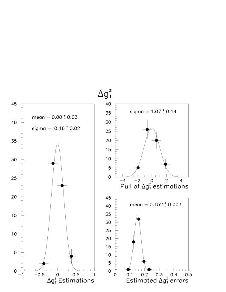
Figure 9: The sampling, pull and error distribution of $\Delta g_{1}^{z}$ estimation by a binned Optimal Variable fit using the proposed in this paper Clustering procedure.

The proposed Multidimensional Clustering technique is a general purpose procedure which can be used in any binned fit provided that the metric matrix is properly defined. As a demonstration, the properties of the estimations of a single coupling ($\delta g_{1}^{z}$) are shown in figure 9 and figure 10. These are the results of two dimensional binned extended likelihood fits, using either the Optimal Variables or the angular distributions of the hadronic and leptonic part of the event [4] [11]. Results (mean of the sampling distributions, mean and sigmas of the pull distributions and expected errors ) concerning the other couplings can be found in Table 3 in comparison to the results which could be obtained by a ”perfect” unbinned extended likelihood.

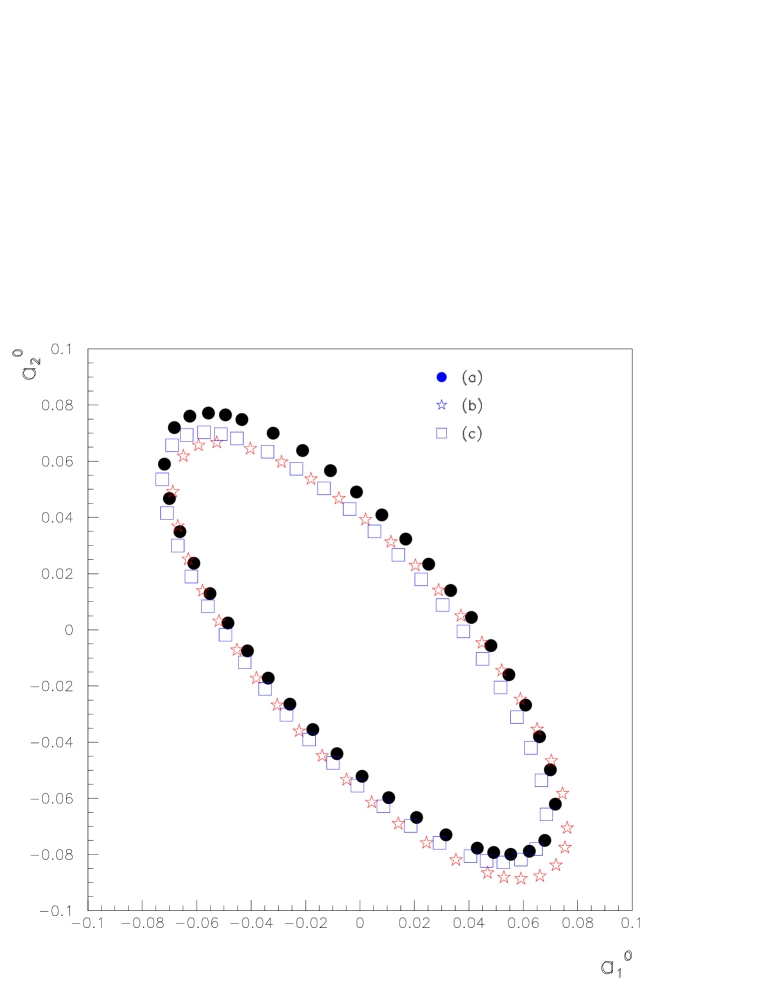
Figure 11: Comparison of confidence intervals in the ($\lambda,\Delta g_{1}^{z}$) plane obtained by : a) an Iterative Optimal Variable, b) Multidimensional Clustering using mega-bins and c) Unbinned extended likelihood (assuming a “perfect” detector) estimation of the couplings.

Finally the extension of the Multidimensional Clustering technique involving grouping of the data points was applied to a data set of 6000 events. The data were divided in 64 groups by the K-means clustering algorithm and the mega-bins were defined by the centers of the data clusters. Results of this method in estimating the ($\lambda_{\gamma},\Delta g^{Z}_{1}$) couplings are shown in figure 11 in comparison with the results of the Iterative Optimal Variable technique (employing the same number of bins) and the “perfect” unbinned extended likelihood fit.

5 Conclusions

In this paper the Optimal Variable technique [1] was generalized in order to be applied for a simultaneous estimation of two couplings using the appropriate TGC model [2]. Two generalization schemes were proposed; one Iterative 2-dimensional procedure which is based on expanding the p.d.f. in a Taylor series and another which is a method of representing the p.d.f. in five dimensions using the real data-points as seeds. The latter is a novel kernel-type algorithm which can be used for any number of real events. Both the techniques were demonstrated to be asymptotically consistent estimators, including the detector effects and the background contribution.

The properties of the techniques when fitting finite size event samples were investigated by M.C. experimentation. Sets of M.C. events, of the same size as the data samples accumulated by each of the LEP experiments at the 183 GeV run, were fitted by both the proposed methods to estimate the $\{\lambda_{\gamma},\Delta g_{1}^{z}\}$ and $\{\Delta\kappa_{\gamma},\Delta g_{1}^{z}\}$ couplings. The distributions of these estimations support the optimal behavior (unbiasedness, consistent error matrix evaluation) of the techniques. Moreover a comparison with the unbinned extended likelihood results demonstrates that the Iterative Optimal Variable and Multidimensional Clustering estimators are practically reaching the maximum sensitivity, as it is shown in Tables 1 and 2. A deterioration of their sensitivity (up to 20%) when dealing with realistic detectors is due to the imperfect resolution of the measuring apparatus.
A comparison [12] between the sensitivity of several multiparametric TGC estimators, which include detector effects, shows that the proposed techniques are equivalent to the Modified Observables [5] technique whilst outperform classical methods of one or two dimensional binned likelihood fits [12].

Finally, in Table 3 the expected sensitivities of the Clustering technique when applied to single coupling estimations are summarized. This method is a general purpose procedure of representing any projection of the probability distribution functions. In this study the $\Delta g_{1}^{z},\lambda_{\gamma}$ and $\Delta\kappa_{\gamma}$ couplings were estimated by using projections of the p.d.f. (6) to the Optimal Variable plane and to the plane defined by the cosines of the polar angles of the hadronic system and the charged lepton ($cos{\Theta_{W}},cos{\Theta_{l}}$). Naturally, the estimations corresponding to the Optimal Variable choice are more sensitive to that of the angular distributions due to the information content [1] of the projected p.d.f.. These results of the 2-dimensional fits with the Clustering procedure are completely equivalent to the results obtained [12] by the standard binned analysis when using the same p.d.f. projections.

	$\lambda\gamma$ - $\Delta g_{1}^{z}$
	$\sigma_{\lambda\gamma}$	$\sigma_{\Delta g_{1}^{z}}$	$\rho$
”Perfect” Extended Likelihood	0.21 $\pm$ 0.01	0.20 $\pm$ 0.01	-0.73 $\pm$ 0.06
Clustering (”Perfect”)	0.21 $\pm$ 0.01	0.20 $\pm$ 0.01	-0.74 $\pm$ 0.06
Iterative estimations (”Perfect” )	0.22 $\pm$ 0.01	0.21 $\pm$ 0.01	-0.74 $\pm$ 0.06
Clustering	0.23 $\pm$ 0.01	0.22 $\pm$ 0.01	-0.74 $\pm$ 0.06
Iterative estimations	0.24 $\pm$ 0.01	0.23 $\pm$ 0.01	-0.72 $\pm$ 0.06

Table 1: Comparison of the statistical properties of the techniques proposed in this paper with the unbinned extended likelihood estimations of the $\lambda_{\gamma}-\Delta g_{1}^{z}$ couplings.

	$\Delta k\gamma$ - $\Delta g_{1}^{z}$
	$\sigma_{\Delta k\gamma}$	$\sigma_{\Delta g_{1}^{z}}$	$\rho$
”Perfect” Extended Likelihood	0.35 $\pm$ 0.03	0.14 $\pm$ 0.01	-0.22 $\pm$ 0.08
Clustering (”Perfect” )	0.35 $\pm$ 0.03	0.15 $\pm$ 0.01	-0.21 $\pm$ 0.09
Iterative estimations (”Perfect” )	0.36 $\pm$ 0.03	0.15 $\pm$ 0.01	-0.24 $\pm$ 0.09
Clustering	0.41 $\pm$ 0.03	0.15 $\pm$ 0.01	-0.23 $\pm$ 0.10
Iterative estimations	0.43 $\pm$ 0.03	0.16 $\pm$ 0.01	-0.27 $\pm$ 0.10

Table 2: Comparison of the statistical properties of the techniques proposed in this paper with the unbinned extended likelihood estimations of the $\Delta\kappa_{\gamma}-\Delta g_{1}^{z}$ couplings.

	$\Delta g_{1}^{z}$	$\lambda_{\gamma}$	$\Delta\kappa_{\gamma}$
”Perfect” Extended Likelihood
mean of estimations	0.006 $\pm$ 0.020	-0.006 $\pm$ 0.02	0.004 $\pm$ 0.06
estimation accuracy	0.14 $\pm$ 0.01	0.16 $\pm$ 0.02	0.49 $\pm$ 0.05
Clustering technique (Opt. Var.)
mean of estimations	0.00 $\pm$ 0.03	-0.01 $\pm$ 0.02	-0.02 $\pm$ 0.09
estimation accuracy	0.16 $\pm$ 0.02	0.16 $\pm$ 0.02	0.47$\pm$ 0.07
pull sigma	1.07 $\pm$ 0.14	0.95 $\pm$ 0.11	1.13 $\pm$ 0.15
Clustering technique (cos$\theta_{W},cos\theta_{l}$)
mean of estimations	-0.01 $\pm$ 0.03	-0.01 $\pm$ 0.02	-0.01 $\pm$ 0.08
estimation accuracy	0.18 $\pm$ 0.02	0.19 $\pm$ 0.02	0.56$\pm$ 0.05
pull sigma	1.05 $\pm$ 0.11	1.1 $\pm$ 0.11	1.13 $\pm$ 0.11

Table 3: Comparison of the statistical properties of the Clustering procedure proposed in this paper with the single unbinned extended likelihood estimations of the $\Delta g_{1}^{z}$, $\lambda_{\gamma}$ and $\Delta\kappa_{\gamma}$.

Figure 1: Deviations of the estimated coupling values ($\hat{\alpha}_{1}=\hat{\lambda}_{\gamma}$, $\hat{\alpha}_{2}=\Delta\hat{g}_{1}^{z}$) from the expansion values.

a) ($\hat{\lambda}_{\gamma}-\lambda_{\gamma}^{0}$) as a function of {$\lambda_{\gamma}^{0}$,$\Delta g_{1}^{z^{0}}\}$,
b) the intersection of (a) with the plane corresponding to zero deviation,
c)($\Delta\hat{g}_{1}^{z}-\Delta g_{1}^{z^{0}}$) as a function of $\{\lambda_{\gamma}^{0},\Delta g_{1}^{z^{0}}\}$,
d) the intersection of (c) with the plane corresponding to zero deviation.
The fitted events have been produced with S.M. couplings. The stars at (b) and (d) indicate the point where both the deviations are zero.

Figure 2: Deviations of the estimated coupling values ($\hat{\alpha}_{1}=\hat{\lambda}_{\gamma}$, $\hat{\alpha}_{2}=\Delta\hat{g}_{1}^{z}$) from the expansion values. The fitted events in [a,b,c,d] have been produced with $\{\lambda_{\gamma}=-1,\Delta g_{1}^{z}=0\}$ whilst [e,f,g,h] correspond to events produced with $\{\lambda_{\gamma}=1$ ,$\Delta g_{1}^{z}=0\}$.

[a,e] $(\hat{\lambda}_{\gamma}-\lambda_{\gamma}^{0})$ as a function of $\{\lambda_{\gamma}^{0}$ , $\Delta g_{1}^{z^{0}}\}$,
[b,f] the intersection of [a,e] with the plane corresponding to zero deviation respectively,
[c,g] $(\Delta\hat{g}_{1}^{z}-\Delta g_{1}^{z^{0}})$ as a function of $\{\lambda_{\gamma}^{0}$, $\Delta g_{1}^{z^{0}}\}$,
[d,h] The intersection of [c,g] with the plane corresponding to zero deviation respectively.
The stars to [b,d] and [f,h] indicate the point where the estimated couplings are equal to the expansion values.

Figure 3: The mean values of the functions a)$\frac{c_{10}(\vec{V})}{c_{00}(\vec{V})}$, b)$\frac{c_{01}(\vec{V})}{c_{00}(\vec{V})}$, c)$\frac{c_{20}(\vec{V})}{c_{00}(\vec{V})}$, d)$\frac{c_{02}(\vec{V})}{c_{00}(\vec{V})}$ and e)$\frac{c_{11}(\vec{V})}{c_{00}(\vec{V})}$ evaluated using M.C. events produced with zero couplings and have been reconstructed with kinematical vectors $\vec{\Omega}$ corresponding to a bin of a)$\frac{c_{10}(\vec{\Omega})}{c_{00}(\vec{\Omega})}$, b)$\frac{c_{01}(\vec{\Omega})}{c_{00}(\vec{\Omega})}$, c)$\frac{c_{20}(\vec{\Omega})}{c_{00}(\vec{\Omega})}$, d)$\frac{c_{02}(\vec{\Omega})}{c_{00}(\vec{\Omega})}$ and e)$\frac{c_{11}(\vec{\Omega})}{c_{00}(\vec{\Omega})}$ respectively.

Figure 4: The distributions of $\chi^{2}$ (n.d.f.=2) probabilities in obtaining $\lambda$ [a,b,e,f] and $\delta$ [c,d,g,h] values in $\{\lambda_{\gamma}$,$\Delta g_{1}^{z}\}$ [a,b,c,d] and $\{\Delta\kappa_{\gamma}$,$\Delta g_{1}^{z}\}$ [e,f,g,h] estimations by the Iterative Optimal Variable technique. The lines with slopes consistent with zero in [a,c,e,g] are first degree polynomial fits to the bootstrap results.

Figure 5: The inclusive event distributions with respect to the five Optimal Variables.The events have been produced with Standard Model couplings.

Figure 6: The distributions of $\chi^{2}$ (n.d.f.=2) probabilities in obtaining $\lambda$ [a,b,e,f] and $\delta$ [c,d,g,h] values in $\{\lambda_{\gamma}$,$\Delta g_{1}^{z}\}$ [a,b,c,d] and $\{\Delta\kappa_{\gamma}$,$\Delta g_{1}^{z}\}$ [e,f,g,h] estimations by the Clustering technique. The lines with slopes consistent with zero in [a,c,e, g] are first degree polynomial fits to the bootstrap results.

Figure 7: Confidence interval estimations with the Iterative Optimal Variable technique. The distributions of errors [a,b,d,e] and correlations [c,f] in estimating the $\{\lambda_{\gamma},\Delta g_{1}^{z}\}$ [a,b,c] and $\{\Delta\kappa_{\gamma},\Delta g_{1}^{z}\}$ [d,e,f] pair of couplings. The data points correspond to the 60 independent data sets whilst the histograms to the bootstrap results. The arrows indicate the average sensitivities summarized in Table 1 and 2.

Figure 8: Confidence interval estimations with the Clustering technique. The distributions of errors [a,b,d,e] and correlations [c,f] in estimating the $\{\lambda_{\gamma},\Delta g_{1}^{z}\}$ [a,b,c] and $\{\Delta\kappa_{\gamma},\Delta g_{1}^{z}\}$ [d,e,f] pair of couplings. The data points correspond to the 60 independent data sets whilst the histograms to the bootstrap results. The arrows indicate the average sensitivities summarized in Table 1 and 2.

Figure 10: The sampling, pull and error distribution od $\Delta g_{1}^{z}$ estimation by a binned $\{cos{\Theta_{W}},cos{\Theta_{l}}\}$ fit using the proposed in this paper Clustering procedure.

References

- [1] G.K. Fanourakis, D.A. Fassouliotis and S.E. Tzamarias, Accurate Estimation of the Trilinear Gauge Couplings using Optimal Observables including Detector effects, HEP-EX/9711015 to appear in NIM A (1998), DELPHI 97-91 PHYS 715
- [2] G. Gounaris, J.-L. Kneur and D. Zeppenfeld, in Physics at LEP2, eds G. Altarelli, T. Sjostrand and F. Zwinger, CERN 96-01 Vol. 1,525(1996)
-
[3]
M. Diehl and O. Nachtmann, Z. Phys. C62 (1994) 397
C.G. Papadopoulos Phys. Let. B386 (1996) 442
M. Diehl and O. Nachtman, HD-THEP-97-03,CPTH-S494-0197,hep-ph/9702208 (1997) -
[4]
P. Abreu et al Measurement of Trilinear Gauge
Couplings in e+e- Collisions at 161GeV and 172 GeV CERN-PPE/97-163
Phys.Lett. B423 (1998) 194
P. Abreu et al. Measurement of the W-pair cross-section and of the W mass in e+e- interactions at 172GeV CERN-PPE/97-160 E.Phys.J. C2(1998) 581 - [5] G. K. Fanourakis et al Extended Modified Observable Technique for a Multi-parametric Trilinear Gauge Coupling Estimation at LEP II DELPHI 98-149 PHYS 793
- [6] G.K. Fanourakis, D.A. Fassouliotis and S.E. Tzamarias, Reweighting Technique for Monte Carlo Integration., DELPHI note 97-56 PHYS 706 (1997).
-
[7]
ERATO: event generator for four-fermion production at LEP II energies and beyond
C. G. Papadopoulos, Comp. Phys. Comm. 101, (1997) 183.
The part of the ERATO code which calculates the coefficients
of the polynomial representation of the matrix elements was extracted and used in
the methods proposed in this paper.
- [8] T. Sjöstrand, PYTHIA 5.6 and JETSET 7.3, CERN-TH/6488-92.
- [9] F.A. Berends, R. Kleis and R. Pittau, EXCALIBUR, Physics at LEP2, eds G. Altarelli, G. T. Sjostrand and F. Zwinger, CERN 96-01 Vol. 2, 23(1996)
- [10] DELSIM Reference Manual, DELPHI note, DELPHI 87-97 PROG-100
- [11] T.J.V Bowcock et al, Measurement of Trilinear Gauge Boson Couplings WWV in e+e- Collisions at 183 GeV, DELPHI 98-94 CONF 162
- [12] G. K. Fanourakis et al Comparison of Trilinear Gauge Couplings Estimation Techniques DELPHI 98-154 PHYS 797
- [13] See for example Neural Networks for Pattern Recognition by C. M. Bishop, Clarendon Press-Oxford (1995)
- [14] M. Rosenblatt, Remarks on some nonparametric estimates of a density function, Annals of Mathematical Statistics 27,(1956)832-837
- [15] J. Moody and C.J. Darken Fast learning in networks of locally-tuned processing units., Neural Computation 1(2), (1989), 281-294.
-
[16]
DELPHI Collaboration: P. Abreu et al., Nucl. Instr. & Meth.
A303 (1991) 233
DELPHI Collaboration: P. Abreu et al., Nucl. Instr. & Meth. A378 (1996) 57 - [17] See for example Statistical Methods in Experimental Physics, W.T. Eadie et al, North-Holland P.C. (1988).
-
[18]
See for example
B. Efron, Better bootstrap confidence intervals, Journal of the American Statistical Association, Vol 82, No. 397, (1987), 171-185.
An Introduction to the Bootstrap (Monographs on Statistics and Applied Probability, No 57) by Bradley Efron and Robert J. Tibshirani, Published by Chapman and Hall