Study of 3-prong hadronic $\tau$ decays with charged kaons

Abstract

Using a sample of 4.7 $fb^{-1}$ integrated luminosity accumulated with the CLEO-II detector at the Cornell Electron Storage Ring (CESR), we have measured the ratios of branching fractions ${\cal B}(\tau^{-}\rightarrow K^{-}h^{+}\pi^{-}\nu_{\tau})/{\cal B}(\tau^{-}\rightarrow h^{-}h^{+}h^{-}\nu_{\tau})=(5.16\pm 0.20\pm 0.50)\times 10^{-2}$, ${\cal B}(\tau^{-}\rightarrow K^{-}h^{+}\pi^{-}\pi^{0}\nu_{\tau})/{\cal B}(\tau^{-}\rightarrow h^{-}h^{+}h^{-}\pi^{0}\nu_{\tau})=(2.54\pm 0.44\pm 0.39)\times 10^{-2}$, ${\cal B}(\tau^{-}\rightarrow K^{-}K^{+}\pi^{-}\nu_{\tau})/{\cal B}(\tau^{-}\rightarrow h^{-}h^{+}h^{-}\nu_{\tau})=(1.52\pm 0.14\pm 0.29)\times 10^{-2}$, and the upper limit: ${\cal B}(\tau^{-}\rightarrow K^{-}K^{+}\pi^{-}\pi^{0}\nu_{\tau})/{\cal B}(\tau^{-}\rightarrow h^{-}h^{+}h^{-}\pi^{0}\nu_{\tau})<0.0154$ at 95% C.L. Coupled with additional experimental information, we use our results to extract information on the structure of three-prong tau decays to charged kaons.

S. J. Richichi,¹ H. Severini,¹ P. Skubic,¹ A. Undrus,¹ M. Bishai,² S. Chen,² J. Fast,² J. W. Hinson,² N. Menon,² D. H. Miller,² E. I. Shibata,² I. P. J. Shipsey,² S. Glenn,³ Y. Kwon,^3, A.L. Lyon,³ S. Roberts,³ E. H. Thorndike,³ C. P. Jessop,⁴ K. Lingel,⁴ H. Marsiske,⁴ M. L. Perl,⁴ V. Savinov,⁴ D. Ugolini,⁴ X. Zhou,⁴ T. E. Coan,⁵ V. Fadeyev,⁵ I. Korolkov,⁵ Y. Maravin,⁵ I. Narsky,⁵ R. Stroynowski,⁵ J. Ye,⁵ M. Artuso,⁶ E. Dambasuren,⁶ S. Kopp,⁶ G. C. Moneti,⁶ R. Mountain,⁶ S. Schuh,⁶ T. Skwarnicki,⁶ S. Stone,⁶ A. Titov,⁶ G. Viehhauser,⁶ J.C. Wang,⁶ J. Bartelt,⁷ S. E. Csorna,⁷ K. W. McLean,⁷ S. Marka,⁷ Z. Xu,⁷ R. Godang,⁸ K. Kinoshita,⁸ I. C. Lai,⁸ P. Pomianowski,⁸ S. Schrenk,⁸ G. Bonvicini,⁹ D. Cinabro,⁹ R. Greene,⁹ L. P. Perera,⁹ G. J. Zhou,⁹ S. Chan,¹⁰ G. Eigen,¹⁰ E. Lipeles,¹⁰ J. S. Miller,¹⁰ M. Schmidtler,¹⁰ A. Shapiro,¹⁰ W. M. Sun,¹⁰ J. Urheim,¹⁰ A. J. Weinstein,¹⁰ F. Würthwein,¹⁰ D. W. Bliss,¹¹ D. E. Jaffe,¹¹ G. Masek,¹¹ H. P. Paar,¹¹ E. M. Potter,¹¹ S. Prell,¹¹ V. Sharma,¹¹ D. M. Asner,¹² J. Gronberg,¹² T. S. Hill,¹² D. J. Lange,¹² R. J. Morrison,¹² H. N. Nelson,¹² T. K. Nelson,¹² D. Roberts,¹² B. H. Behrens,¹³ W. T. Ford,¹³ A. Gritsan,¹³ H. Krieg,¹³ J. Roy,¹³ J. G. Smith,¹³ J. P. Alexander,¹⁴ R. Baker,¹⁴ C. Bebek,¹⁴ B. E. Berger,¹⁴ K. Berkelman,¹⁴ V. Boisvert,¹⁴ D. G. Cassel,¹⁴ D. S. Crowcroft,¹⁴ M. Dickson,¹⁴ S. von Dombrowski,¹⁴ P. S. Drell,¹⁴ K. M. Ecklund,¹⁴ R. Ehrlich,¹⁴ A. D. Foland,¹⁴ P. Gaidarev,¹⁴ R. S. Galik,¹⁴ L. Gibbons,¹⁴ B. Gittelman,¹⁴ S. W. Gray,¹⁴ D. L. Hartill,¹⁴ B. K. Heltsley,¹⁴ P. I. Hopman,¹⁴ J. Kandaswamy,¹⁴ D. L. Kreinick,¹⁴ T. Lee,¹⁴ Y. Liu,¹⁴ N. B. Mistry,¹⁴ C. R. Ng,¹⁴ E. Nordberg,¹⁴ M. Ogg,^14, J. R. Patterson,¹⁴ D. Peterson,¹⁴ D. Riley,¹⁴ A. Soffer,¹⁴ B. Valant-Spaight,¹⁴ C. Ward,¹⁴ M. Athanas,¹⁵ P. Avery,¹⁵ C. D. Jones,¹⁵ M. Lohner,¹⁵ S. Patton,¹⁵ C. Prescott,¹⁵ A. I. Rubiera,¹⁵ J. Yelton,¹⁵ J. Zheng,¹⁵ G. Brandenburg,¹⁶ R. A. Briere,¹⁶ A. Ershov,¹⁶ Y. S. Gao,¹⁶ D. Y.-J. Kim,¹⁶ R. Wilson,¹⁶ H. Yamamoto,¹⁶ T. E. Browder,¹⁷ Y. Li,¹⁷ J. L. Rodriguez,¹⁷ S. K. Sahu,¹⁷ T. Bergfeld,¹⁸ B. I. Eisenstein,¹⁸ J. Ernst,¹⁸ G. E. Gladding,¹⁸ G. D. Gollin,¹⁸ R. M. Hans,¹⁸ E. Johnson,¹⁸ I. Karliner,¹⁸ M. A. Marsh,¹⁸ M. Palmer,¹⁸ M. Selen,¹⁸ J. J. Thaler,¹⁸ K. W. Edwards,¹⁹ A. Bellerive,²⁰ R. Janicek,²⁰ P. M. Patel,²⁰ A. J. Sadoff,²¹ R. Ammar,²² P. Baringer,²² A. Bean,²² D. Besson,²² D. Coppage,²² C. Darling,²² R. Davis,²² S. Kotov,²² I. Kravchenko,²² N. Kwak,²² L. Zhou,²² S. Anderson,²³ Y. Kubota,²³ S. J. Lee,²³ R. Mahapatra,²³ J. J. O’Neill,²³ R. Poling,²³ T. Riehle,²³ A. Smith,²³ M. S. Alam,²⁴ S. B. Athar,²⁴ Z. Ling,²⁴ A. H. Mahmood,²⁴ S. Timm,²⁴ F. Wappler,²⁴ A. Anastassov,²⁵ J. E. Duboscq,²⁵ K. K. Gan,²⁵ T. Hart,²⁵ K. Honscheid,²⁵ H. Kagan,²⁵ R. Kass,²⁵ J. Lee,²⁵ H. Schwarthoff,²⁵ M. B. Spencer,²⁵ A. Wolf,²⁵ and M. M. Zoeller²⁵

I Introduction

Decays of the $\tau$ lepton present a unique opportunity to confirm and further probe the Standard Model. The large mass of the $\tau$ lepton makes possible decays into hadrons in an environment where the initial state is simple and well understood[1]. This allows comparison with hadron production at comparable center of mass energies from processes such as pion-nucleon, nucleon-nucleon and electron-positron collisions. Strange $\tau$ decays give us information on $SU(3)_{f}$ symmetry breaking, and direct measurements of the Cabibbo angle ($\theta_{c}$). Alternately, the rates for such Cabibbo-suppressed decays (e.g., $\tau\to K\nu_{\tau},\tau\to K^{*}\nu_{\tau}$, and $\tau\to K_{1}\nu_{\tau}$) can be predicted using corresponding measurements of the Cabibbo favored modes ($\tau\to\pi\nu_{\tau}$, $\tau\to\rho\nu_{\tau}$, and $\tau\to a_{1}\nu_{\tau}$). For the case of vector coupling, the theoretically expected ratio of branching ratios, ${\cal B}(\tau\to K^{*}\nu_{\tau})/{\cal B}(\tau\to\rho\nu_{\tau})$[2] can be written following the approach of the Das-Mathur-Okubo sum rules[3] as $f(m_{K^{*}},m_{\rho},m_{\tau})\tan^{2}\theta_{c}g_{K^{*}}^{2}/g_{\rho}^{2}$, where $f$ is a factor that incorporates the phase space available for decays into $\rho$ and $K^{*}$, $\theta_{c}$ is the Cabibbo angle, and the factors $g_{K^{*}}$ and $g_{\rho}$ reflect the coupling strengths of the $K^{*}$ and $\rho$ to the vector current. In the limit of exact SU(3) symmetry, there is no differentiation between the $K^{*}$ and the $\rho$, so $g_{K^{*}}=g_{\rho}$. In the more realistic case of broken symmetry, however, the couplings $g$ are directly proportional to mass. In this approximation, using $\sin\theta_{c}$=0.221 [4], the ratio of rates equals 0.068. There are many experimental results for $\tau\to K^{*}\nu_{\tau}$ (where the charged $K^{*}$ is observed through the very clean decay chain: $K^{*}\to K^{0}_{S}\pi$; $K^{0}_{S}\to\pi^{+}\pi^{-}$) which are in agreement with this prediction[4].

We expect similar relationships to hold for the coupling of the tau to the axial vector $K_{1}$ resonance relative to the $a_{1}$ resonance. Unfortunately, $\tau\to K_{1}\nu_{\tau}$ is not as well-studied as $\tau\to K^{*}\nu_{\tau}$, in part due to the fact that the $K_{1}$ decay most often leads to multi-prong events that include charged kaons. Whereas the $K^{*}$ can be unambiguously identified through its decay, $K^{*}\to K^{0}_{S}\pi$, a measurement of charged kaons requires good K/$\pi$ particle identification in order to separate kaons from the substantially more numerous pions. Moreover, theoretical understanding of charged kaon production in tau decay is hampered by uncertainties in the production mechanism; there is a wide range of predictions for the mass spectrum (expected to be dominated by $K_{1}(1270)$ and $K_{1}(1400)$), the $K^{*}\pi/K\rho$ ratio (in $K\pi\pi$), and the helicity amplitudes for $\tau$ decays to kaons.

In recent years the large data samples accumulated at CLEO and LEP have allowed much-improved measurements of inclusive decays of tau leptons to charged kaons, complementing similar measurements of inclusive decays of tau leptons to neutral kaons. In this analysis we measure the ratio of branching fractions of $\tau^{-}\rightarrow K^{-}h^{+}\pi^{-}(\pi^{0})\nu_{\tau}$ and $\tau^{-}\rightarrow K^{-}K^{+}\pi^{-}(\pi^{0})\nu_{\tau}$ relative to $\tau^{-}\rightarrow h^{-}h^{+}h^{-}(\pi^{0})\nu_{\tau}$, where $h^{\pm}$ can be either a charged pion or kaon. The decay $\tau\to K^{-}\pi^{+}\pi^{-}(\pi^{0})\nu_{\tau}$ proceeding through the $K^{-}K^{0}(\pi^{0})\nu_{\tau}$ intermediate state has been measured in [5]; in our analysis, these are considered background since we are interested in studying tau decays directly into 3 or 4 mesons that include charged kaons.

II Data sample and event selection

Our data sample contains approximately 4.3 million $\tau$-pairs produced in $e^{+}e^{-}$ collisions, corresponding to an integrated luminosity of 4.7 $fb^{-1}$. The data were collected with the CLEO-II detector[6] at the Cornell Electron Storage Ring operating at a center-of-mass energy approximately 10.58 GeV.

The CLEO II detector is a general purpose solenoidal magnet spectrometer and calorimeter. The detector was designed for efficient triggering and reconstruction of two-photon, tau-pair, and hadronic events. Measurements of charged particle momenta are made with three nested coaxial drift chambers consisting of 6, 10, and 51 layers, respectively. These chambers fill the volume from $r$=3 cm to $r$=1 m, with $r$ the radial coordinate relative to the beam (${\hat{z}}$) axis. This system is very efficient ($\epsilon\geq$98%) for detecting tracks that have transverse momenta ($p_{T}$) relative to the beam axis greater than 200 MeV/$c$, and that are contained within the good fiducial volume of the drift chamber ($|\cos\theta|<$0.94, with $\theta$ defined as the polar angle relative to the beam axis). The charged particle detection efficiency in the fiducial volume decreases to approximately 90% at $p_{T}\sim$100 MeV/$c$. For $p_{T}<$100 MeV/$c$, the efficiency decreases roughly linearly to zero at a threshold of $p_{T}\approx$30 MeV/$c$. This system achieves a momentum resolution of $(\delta p/p)^{2}=(0.0015p)^{2}+(0.005)^{2}$ ($p$ is the momentum, measured in GeV/$c$). Pulse height measurements in the main drift chamber provide specific ionization ($dE/dx$) resolution of 5.5% for Bhabha events, giving good $K/\pi$ separation for tracks with momenta up to 700 MeV/$c$ and separation nearly 2$\sigma$ in the relativistic rise region above 2 GeV/$c$. Outside the central tracking chambers are plastic scintillation counters, which are used as a fast element in the trigger system and also provide particle identification information from time-of-flight measurements.

Beyond the time-of-flight system is the electro-magnetic calorimeter, consisting of 7800 thallium-doped CsI crystals. The central “barrel” region of the calorimeter covers about 75% of the solid angle and has an energy resolution which is empirically found to follow:

$$~{}~{}~{}~{}~{}~{}~{}~{}~{}~{}~{}~{}~{}~{}~{}~{}~{}~{}~{}~{}~{}~{}~{}~{}~{}~{}~{}~{}~{}\frac{\sigma_{\rm E}}{E}(\%)=\frac{0.35}{E^{0.75}}+1.9-0.1E;$$ (1)

$E$ is the shower energy in GeV. This parameterization includes effects such as noise, and translates to an energy resolution of about 4% at 100 MeV and 1.2% at 5 GeV. Two end-cap regions of the crystal calorimeter extend solid angle coverage to about 95% of $4\pi$, although energy resolution is not as good as that of the barrel region. The tracking system, time of flight counters, and calorimeter are all contained within a superconducting coil operated at 1.5 Tesla. Flux return and tracking chambers used for muon detection are located immediately outside the coil and in the two end-cap regions.

We select $e^{+}e^{-}\to\tau^{+}\tau^{-}$ events having a “1vs3” topology in which one $\tau$ lepton decays into one charged particle (plus possible neutrals), and the other $\tau$ lepton decays into 3 charged hadrons (plus possible neutrals). An event is separated into two hemispheres based on the measured event thrust axis. Loose cuts on ionization measured in the drift chamber, energy deposited in the calorimeter and the maximum penetration depth into the muon detector system are applied to charged tracks in the signal (3-prong) hemisphere to reject leptons. Backgrounds from $\tau$ and hadronic events with $K_{S}^{0}$ are suppressed by requirements on the impact parameters of charged tracks. To reduce the background from two-photon collisions ($e^{+}e^{-}\to e^{+}e^{-}\gamma\gamma$ with $\gamma\gamma\to$hadrons or $\gamma\gamma\to l^{+}l^{-}$), cuts on visible energy ($E_{vis}$) and total event transverse momentum ($P_{t}$) are applied: 2.5 GeV $<E_{vis}<10$ GeV, and $P_{t}>$0.3 GeV/$c$. We also require the invariant mass of the tracks and showers in the 3-prong hemisphere, calculated under the $\pi^{-}\pi^{+}\pi^{-}$ hypothesis, to be less than 1.7 GeV/$c$.

Events are accepted for which the tag hemisphere (1-prong side) is consistent with one of the following four decays: $\tau^{+}\rightarrow e^{+}\nu_{e}{\overline{\nu}_{\tau}}$, $\tau^{+}\rightarrow\mu^{+}\nu_{\mu}{\overline{\nu}_{\tau}}$, $\tau^{+}\rightarrow\pi^{+}{\overline{\nu}_{\tau}}$, or $\tau^{+}\rightarrow\rho^{+}{\overline{\nu}_{\tau}}$.

For the $\tau^{-}\rightarrow K^{-}h^{+}\pi^{-}(\pi^{0})\nu_{\tau}$ analysis, we determine the kaon and pion yields, using the two same-sign tracks from the three-prong hemisphere. For the $\tau^{-}\rightarrow K^{-}K^{+}\pi^{-}(\pi^{0})\nu_{\tau}$ mode, only the track having sign opposite to its parent $\tau$ is considered as a candidate kaon. Note that we implicitly assume that all signal kaons originating from $\tau$ decays in our selected 1vs3 samples come from one of the decay modes $\tau^{-}\rightarrow K^{-}\pi^{+}\pi^{-}\nu_{\tau}$, $\tau^{-}\rightarrow K^{-}K^{+}\pi^{-}\nu_{\tau}$, $\tau^{-}\rightarrow K^{-}\pi^{+}\pi^{-}\pi^{0}\nu_{\tau}$, or $\tau^{-}\rightarrow K^{-}K^{+}\pi^{-}\pi^{0}\nu_{\tau}$. The decays $\tau^{-}\rightarrow\pi^{-}K^{+}\pi^{-}\nu_{\tau}$ and $\tau^{-}\rightarrow K^{-}\pi^{+}K^{-}\nu_{\tau}$ are extremely small in the Standard Model and have not been experimentally observed, and the decay rate for $\tau^{-}\rightarrow K^{-}K^{+}K^{-}\nu_{\tau}$ is expected be $\sim 1\%$ relative to that for $\tau^{-}\rightarrow K^{-}\pi^{+}\pi^{-}\nu_{\tau}$ due to the limited phase space and the low probability of $(s\bar{s})$ popping.

Candidate events with and without $\pi^{0}$’s are distinguished by the characteristics of showers in the electro-magnetic calorimeter. A ‘photon’ candidate is defined as a shower in the barrel region of the electromagnetic calorimeter with energy above 40 MeV and having an energy deposition pattern consistent with true photons. It must be separated from the closest charged track by at least 30 cm (20 cm for photons used in $\pi^{0}$ reconstruction). $\tau^{-}\to K^{-}h^{+}\pi^{-}\nu_{\tau}$ and $\tau^{-}\to K^{-}K^{+}\pi^{-}\nu_{\tau}$ candidates are defined as those events having zero photons with energy above 100 MeV in the 3-prong hemisphere. For the $\tau^{-}\to K^{-}h^{+}\pi^{-}\pi^{0}\nu_{\tau}$ and $\tau^{-}\to K^{-}K^{+}\pi^{-}\pi^{0}\nu_{\tau}$ decay modes there must be at least two photons in the signal hemisphere, but no more than two photon candidates having a shower energy above 100 MeV. The two most energetic photons in this hemisphere are then paired to form $\pi^{0}$ candidates.

III Signal extraction procedure

To find the number of events with kaons, we use specific ionization information from the central drift chamber. For each track we calculate the parameter $\delta_{K}$, defined as the deviation of the measured energy loss relative to that expected for true kaons in units of the measured $dE/dx$ resolution. For true kaons, this variable is distributed as a unit Gaussian centered at 0. For pion tracks, $\delta_{k}$ also has a Gaussian-like shape but with the mean shifted from zero in a momentum-dependent manner. In this analysis we concentrate on those tracks having momentum $p>$1.5 GeV/$c$. Although the $K/\pi$ separation is better at low momenta, we focus on this high momentum region because the separation varies only slowly through this regime and the systematics of signal extraction are therefore more tractable. These tracks generally have the highest momenta of the tracks in the three-prong hemisphere and are well-separated spatially from the lower momentum tracks. Non-$\tau$ background as well as the pion background relative to the desired kaon signal in real $\tau$ decays is also smaller at high momenta.

The number of kaon and pion tracks in the three-prong hemisphere is found statistically by fitting the $\delta_{k}$ distribution for charged tracks in the three-prong hemisphere to the sum of the pion and kaon $\delta_{k}$ shapes. Since the $K-\pi$ separation is modest, it is critical that the shape of the $\delta_{k}$ distribution for pions is well understood. $K_{s}^{0}\rightarrow\pi^{-}\pi^{+}$ decays provide a very clean sample of true pions from which this distribution can be determined from data. For the pion and kaon shapes, we use a Johnson distribution[7, 8] with mean shifted from zero, and a unit Gaussian centered at zero, respectively.

Requirements on the minimum number of hits used in the $dE/dx$ calculation ($>20$, out of a maximum of 49) and the polar angle of the candidate kaon track ($|\cos{\theta}|<0.8$, where $\theta$ is the polar angle of the track relative to the positron beam direction) ensure that the track is contained in the good fiducial volume of the drift chamber and that the $dE/dx$ information for the track is of high quality. Since the $K/\pi$ separation depends on the number of hits ($N_{hit}$), as well as momentum ($p$), we perform separate $\delta_{k}$ fits for 36 different bins in the two parameter ($N_{hit}$, $p$) space. The kaon and pion yields for each momentum bin above our minimum momentum of 1.5 GeV/$c$ are extracted knowing the pion (and kaon) $\delta_{k}$ shapes appropriate for each $N_{hit}$ interval over a specified momentum range. An example of a $\delta_{k}$ fit, showing the kaon and pion components, is displayed in Fig. 1. The $K:\pi$ mixture in this example is typical of the $\tau^{-}\to K^{-}h^{+}\pi^{-}\nu_{\tau}$ analysis (of order $1:20$) and is prepared using all tracks with momenta $1.9$ GeV/$c<p<$2.1 GeV/$c$.

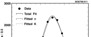
FIG. 1.: Fit to $\delta_{k}$ distribution for charged tracks in the 3-prong hemisphere of candidate $\tau\tau$ events, with the fitted kaon and pion curves overlaid. Open circles are data, the dotted line shows the kaon contribution to the fit, the dashed line shows the pion contribution and the solid line corresponds to the sum of the fitted kaon and pion curves. The confidence level of the fit is 92%; if the kaon contribution is not included, the C.L. is less than $10^{-3}$.

To determine the total number of $\tau\to KX$ events, we must extrapolate from our measured yields in the region $p>$1.5 GeV/$c$ to the lower track momentum region. This is done by fitting the measured kaon and pion momentum spectra to the spectra expected from Monte Carlo (MC) simulations in the $p>$1.5 GeV/$c$ region, and integrating over the full momentum range. Uncertainties in this MC model are included in our systematic error.

FIG. 2.: Reconstructed a) kaon and b) pion momentum spectra for $\tau\rightarrow Kh\pi\nu_{\tau}$ candidates. Solid squares are data points and histogram is the MC shape.

The reconstructed momentum spectrum for the $\tau^{-}\rightarrow K^{-}h^{+}\pi^{-}\nu_{\tau}$ analysis is shown in Fig. 2, with the fit overlaid. For decay modes with $\pi^{0}$ mesons, $\delta_{k}$ distributions are made and fitted separately for cases in which the two-photon invariant mass falls in the $\pi^{0}$ signal and sideband regions. The signal region is taken to be $-4<S_{\gamma\gamma}<3$, and the sidebands defined as $-18<S_{\gamma\gamma}<-10$ and $7<S_{\gamma\gamma}<17$, where $S_{\gamma\gamma}$ is the number of standard deviations from the $\pi^{0}$ mass. Subtracting the $K/\pi$ yields from the $\pi^{0}$ sidebands, the $K/\pi$ signals associated with true $\pi^{0}$ production are determined, and the $\tau^{-}\rightarrow K^{-}h^{+}\pi^{-}\pi^{0}\nu_{\tau}$ yield is extracted. In Table I we summarize the total yields and backgrounds for all four samples.

TABLE I.: Kaon and pion yields in our 1vs3 samples and estimates of background levels. Errors are statistical only. In each pair of numbers in the table the first number pertains to kaons and the second to pions. The $\tau$ feed-across background is included in the $K/\pi$ yields while the hadronic background has already been subtracted.

Hadronic	Number of K/$\pi$	hadronic	$\tau$ feed-
final state	reconstructed	background, %	across, %
$Kh\pi/\pi\pi\pi$	$7903\pm 302$/$294780\pm 1184$	$3.1/0.5$	$9.1/11.2$
$Kh\pi\pi^{0}/\pi\pi\pi\pi^{0}$	$719\pm 123$/$55140\pm 680$	$4.9/0.8$	$9.8/4.5$
$KK\pi/\pi\pi\pi$	$2305\pm 211$/$149599\pm 761$	$5.1/0.4$	$7.0/14.5$
$KK\pi\pi^{0}/\pi\pi\pi\pi^{0}$	$158\pm 89$/$26915\pm 457$	$6.4/0.7$	$0/7.2$

IV Background

There are two primary sources of background: continuum hadronic events ($e^{+}e^{-}\rightarrow q\bar{q}\rightarrow hadrons$) and non-signal $\tau$ decays (“$\tau$ feed-across”). We estimate hadronic background from a continuum hadronic Monte Carlo sample (using the JETSET v7.3[9] event generator and GEANT [10] detector simulation code). The kaon and pion momentum spectra resulting from qq̄ events that satisfy our selection criteria are found from this Monte Carlo sample and subtracted from the data $K/\pi$ spectra prior to fitting for the $\tau\to KX$ and $\tau\to\pi X$ yields. The level of hadronic background is shown in Table I.

$\tau$ decay modes containing $K^{0}_{S}$ mesons are considered feed-across background, because the major source of $\tau$ background to $\tau^{-}\rightarrow K^{-}h^{+}\pi^{-}(\pi^{0})\nu_{\tau}$ is found to be $\tau^{-}\rightarrow K^{-}K^{0}(\pi^{0})\nu_{\tau}$ decays, in which $K^{0}_{S}\to\pi^{+}\pi^{-}$. There is also contamination of modes without $\pi^{0}$’s from modes with $\pi^{0}$’s, and vice versa, which we also determine from Monte Carlo simulations, using our measured branching fractions as inputs. Three prong decays with kaons and more than one $\pi^{0}$ are severely phase space suppressed and are neglected in this analysis. The approximate level of $\tau$ background is also given in Table I.

V Numerical Results

We determine the ratio of branching fractions relative to the normalizing modes directly from the fitted number of kaon and pion tracks in the 1vs3 sample. For the $\tau^{-}\rightarrow K^{-}h^{+}\pi^{-}\nu_{\tau}$ and $\tau^{-}\rightarrow K^{-}h^{+}\pi^{-}\pi^{0}\nu_{\tau}$ decay modes, each event contributes 2 same-sign tracks to the analyzed sample of tracks, one of which is a kaon and one a pion. By contrast, each $\tau^{-}\to\pi^{-}\pi^{+}\pi^{-}\nu_{\tau}$ event contributes 2 pions. Straightforward algebra can be used to find a simple expression for the desired ratio of branching fractions, as outlined in the Appendix. Using this calculation we obtain the results for the ratios ($R$) of branching fractions shown in Table II. The first error shown is statistical and the second is systematic.

TABLE II.: Final results for ratios of branching fractions and derived absolute branching fractions for all four analyses.

Decay Mode	Ratio definition	Value ($\times 10^{-2}$)
$\tau\rightarrow Kh\pi\nu_{\tau}$	${\cal B}(\tau\rightarrow Kh\pi\nu_{\tau})/{\cal B}(\tau\rightarrow\pi\pi\pi\nu_{\tau})$	$5.44\pm 0.21\pm 0.53$
$\tau\rightarrow Kh\pi\pi^{0}\nu_{\tau}$	${\cal B}(\tau\rightarrow Kh\pi\pi^{0}\nu_{\tau})/{\cal B}(\tau\rightarrow\pi\pi\pi\pi^{0}\nu_{\tau})$	$2.61\pm 0.45\pm 0.42$
$\tau\rightarrow KK\pi\nu_{\tau}$	${\cal B}(\tau\rightarrow KK\pi\nu_{\tau})/{\cal B}(\tau\rightarrow\pi\pi\pi\nu_{\tau})$	$1.60\pm 0.15\pm 0.30$
$\tau\rightarrow KK\pi\pi^{0}\nu_{\tau}$	${\cal B}(\tau\rightarrow KK\pi\pi^{0}\nu_{\tau})/{\cal B}(\tau\rightarrow\pi\pi\pi\pi^{0}\nu_{\tau})$	$0.79\pm 0.44\pm 0.16$

VI Systematic errors

The breakdown of systematic errors for each decay mode is given in Table III.

TABLE III.: Systematic errors

Source	Ratio of branching fractions
	$\frac{Kh\pi\nu}{\pi\pi\pi\nu}$	$\frac{Kh\pi\pi^{0}\nu}{\pi\pi\pi\pi^{0}\nu}$	$\frac{KK\pi\nu}{\pi\pi\pi\nu}$	$\frac{KK\pi\pi^{0}\nu}{\pi\pi\pi\pi^{0}\nu}$
Kaon extraction procedure	6%	7%	9%	8%
MC Model uncertainties	2%	6%	9%	15%
$\tau$ MC branching fraction uncertainties	2%	9%	4%	3%
MC statistics (for efficiencies)	1%	3%	2%	4%
qq̄ background	3%	5%	5%	6%
Other backgrounds ($2\gamma$, QED, beam-gas)	5%	5%	5%	5%
Photon finding/veto	4%	6%	10%	6%
Tracking, Trigger, Tag ID	cancels	cancels	cancels	cancels
Total	10%	16%	19%	20%

The dominant systematic errors arise from the uncertainty in the fit procedure used to determine the number of kaons and pions in the 1vs3 sample and from the choice of decay models in Monte Carlo simulation. The former error is estimated by performing cross-checks on independent mixtures of kaons and pions with known fractions of particles of each type. We obtain tagged samples of kaons and pions using data samples of $\phi\rightarrow K^{+}K^{-}$ or $D^{*+}\rightarrow D^{0}\pi^{+}$ events, with the $D^{0}$ decaying to either $K^{-}\pi^{+}$ or $K^{-}\pi^{+}\pi^{-}\pi^{+}$. The $\delta_{k}$ distributions of kaons and pions are added in proportions ranging from 1:1 to 1:25, and the signal extraction procedure applied. The number of fitted kaons is compared to the true number of input kaons and a ratio ($N_{fit}\over N_{true}$) determined. The results of this procedure are used to estimate the systematic errors inherent in the signal extraction procedure. We then extrapolate the results of this cross-check to the mixture appropriate to each specific decay mode and assess the corresponding systematic error of the signal extraction. The expected fractions of kaons in the measured decay modes, averaged over the momentum range $p>$1.5 GeV/$c$, are 1:22, 1:31, 1:49 and 1:34 for the $\tau\to Kh\pi\nu$, $Kh\pi\pi^{0}\nu$, $KK\pi\nu$ and $KK\pi\pi^{0}\nu$ analyses, respectively.

The MC modeling error listed in Table III includes the uncertainty in fitting the extracted pion and kaon momentum spectra (i.e., extrapolating into the $p<$1.5 GeV/$c$ region), as well as the efficiencies for Monte Carlo events to pass both our event and track selection criteria. To evaluate this error, a variety of decay models, both resonant and non-resonant, are used to determine the possible shapes of the $dN\over dp$ spectra and to recalculate branching ratios. The following models were investigated in order to evaluate the systematic error: for $\tau^{-}\to K^{-}\pi^{+}\pi^{-}\nu_{\tau}$: $\tau\to K_{1}(1270)\nu_{\tau}$, $\tau\to K_{1}(1400)\nu_{\tau}$, and phase space; for $\tau^{-}\to K^{-}K^{+}\pi^{-}\nu_{\tau}$: $\tau\to K^{*0}K\nu_{\tau}$, $\tau\to\rho(1690)\nu_{\tau}$ ($\rho(1690)\to K^{*0}K$), and phase space; for $\tau^{-}\to K^{-}\pi^{+}\pi^{+}\pi^{0}\nu_{\tau}$: $\tau\to K\omega\nu_{\tau}$ and phase space; for $\tau^{-}\to K^{-}K^{+}\pi^{-}\pi^{0}\nu_{\tau}$: $\tau\to K^{*}K^{*0}$, $\tau\to\rho(1690)\nu_{\tau}$ ($\rho(1690)\to K^{*}K^{*0}$), and phase space. To obtain central values, the following primary models were used: the model described in [11] for the $\tau\to K\pi\pi\nu_{\tau}$ decay mode (mostly $K_{1}(1400)\to K^{*}\pi$); a mixture of phase space and $\tau\to K\omega\nu_{\tau}$ in proportions 75:25 for the $\tau\to K\pi\pi\pi^{0}\nu_{\tau}$ decay mode; the current KORALB [11] model (including $K^{*}K$ and $\rho K$) for the $\tau\to KK\pi\nu_{\tau}$ decay mode; and a mixture of phase space and $\tau\to K^{*}K^{*0}\nu$ in proportions 50:50 for the $\tau\to KK\pi\pi^{0}\nu_{\tau}$ decay mode. Because $\tau$ decay modes with kaons are not well understood theoretically, and because data on such decays is sparse, this modeling uncertainty is somewhat large.

To determine the systematic error in our feed-across estimate due to the uncertainty in the input tau decay branching fractions, several different samples of generic $\tau$ Monte Carlo were generated using the KORALB package, with branching fractions of the components changed within $\pm 1\sigma$ of the known value. Most feed-across corrections are determined using branching fractions from the Particle Data Group[4]; the magnitude of feed-across corrections internal to this measurement (e.g., $\tau^{-}\to K^{-}\pi^{+}\pi^{-}\pi^{0}\nu_{\tau}$ contamination of $\tau^{-}\to K^{-}\pi^{+}\pi^{-}\nu_{\tau}$) are taken from the results of this analysis. The quoted systematic error is derived from the observed variation of the final results when the input branching fractions are varied.

We conservatively assign a 100% systematic error on the hadronic background level (see Table II), since our hadronic simulation may not accurately model the qq̄ background. Remaining backgrounds, namely 2-photon events, beam-gas interactions, and QED background, are assessed by varying the event and track selection requirements and determined to be less than 5%. To account for systematics related to photon-finding, and the neutral energy veto, we investigate the dependence of the final results upon the particular values of the cuts used in $\pi^{0}$ reconstruction and the photon veto. This study gives 2-10% systematic errors (Table III).

We assign a MC statistics error corresponding to the statistical error on the efficiencies and feed-across corrections determined from Monte Carlo simulations. There are other systematic effects that cancel in the final ratio of branching fractions such as trigger efficiencies, tag identification requirements and track-finding systematics.

VII Summary

We have measured the following ratios of branching fractions:

$${\cal B}(\tau^{-}\rightarrow K^{-}h^{+}\pi^{-}\nu_{\tau})/{\cal B}(\tau^{-}\rightarrow\pi^{-}\pi^{+}\pi^{-}\nu_{\tau})=(5.44\pm 0.21\pm 0.53)\times 10^{-2},\\$$ (2)

$${\cal B}(\tau^{-}\rightarrow K^{-}h^{+}\pi^{-}\pi^{0}\nu_{\tau})/{\cal B}(\tau^{-}\rightarrow\pi^{-}\pi^{+}\pi^{-}\pi^{0}\nu_{\tau})=(2.61\pm 0.45\pm 0.42)\times 10^{-2},$$ (3)

$${\cal B}(\tau^{-}\rightarrow K^{-}K^{+}\pi^{-}\nu_{\tau})/{\cal B}(\tau^{-}\rightarrow\pi^{-}\pi^{+}\pi^{-}\nu_{\tau})=(1.60\pm 0.15\pm 0.30)\times 10^{-2},$$ (4)

$${\cal B}(\tau^{-}\rightarrow K^{-}K^{+}\pi^{-}\pi^{0}\nu_{\tau})/{\cal B}(\tau^{-}\rightarrow\pi^{-}\pi^{+}\pi^{-}\pi^{0}\nu_{\tau})<0.0157(95\%C.L.),$$ (5)

where the limit is quoted because the value in Table II is not statistically significant. Contributions to both denominator and numerator from $\tau\to K^{0}_{S}X$; $K^{0}_{S}(\to\pi^{+}\pi^{-})$ have been excluded. If we instead normalize to $\tau\rightarrow h^{-}h^{+}h^{-}(\pi^{0})\nu_{\tau}$, the corresponding ratio of branching fractions are:

$${\cal B}(\tau^{-}\rightarrow K^{-}h^{+}\pi^{-}\nu_{\tau})/{\cal B}(\tau^{-}\rightarrow h^{-}h^{+}h^{-}\nu_{\tau})=(5.16\pm 0.20\pm 0.50)\times 10^{-2},$$ (6)

$${\cal B}(\tau^{-}\rightarrow K^{-}h^{+}\pi^{-}\pi^{0}\nu_{\tau})/{\cal B}(\tau^{-}\rightarrow h^{-}h^{+}h^{-}\pi^{0}\nu_{\tau})=(2.54\pm 0.44\pm 0.39)\times 10^{-2},$$ (7)

$${\cal B}(\tau^{-}\rightarrow K^{-}K^{+}\pi^{-}\nu_{\tau})/{\cal B}(\tau^{-}\rightarrow h^{-}h^{+}h^{-}\nu_{\tau})=(1.52\pm 0.14\pm 0.29)\times 10^{-2},and$$ (8)

$${\cal B}(\tau^{-}\rightarrow K^{-}K^{+}\pi^{-}\pi^{0}\nu_{\tau})/{\cal B}(\tau^{-}\rightarrow h^{-}h^{+}h^{-}\pi^{0}\nu_{\tau})<0.0154.$$ (9)

Subtracting (8) from (6) and the central value of (9) from (7) we find:

$${\cal B}(\tau^{-}\rightarrow K^{-}\pi^{+}\pi^{-}\nu_{\tau})/{\cal B}(\tau^{-}\rightarrow h^{-}h^{+}h^{-}\nu_{\tau})=(3.64\pm 0.24\pm 0.58)\times 10^{-2},$$ (10)

and

$${\cal B}(\tau^{-}\rightarrow K^{-}\pi^{+}\pi^{-}\pi^{0}\nu_{\tau})/{\cal B}(\tau^{-}\rightarrow h^{-}h^{+}h^{-}\pi^{0}\nu_{\tau})=(1.77\pm 0.62\pm 0.42)\times 10^{-2}.$$ (11)

Using the CLEO measurements of the decay channels $\tau^{-}\to h^{-}h^{+}h^{-}\nu_{\tau}$ and $\tau^{-}\to h^{-}h^{+}h^{-}\pi^{0}\nu_{\tau}$ [12] for the denominator, and Eqns. (8)-(11), we find the branching fractions given in Table IV.

VIII Discussion

The $\tau^{-}\to K^{-}\pi^{+}\pi^{-}\nu_{\tau}$ decay mode is believed to occur predominantly through coupling to the axial-vector mesons $K_{1}(1270)$ and $K_{1}(1400)$. The numerical prediction for the branching fraction of this decay mode calculated by Finkemeier and Mirkes[13] is $0.77\%$, more than twice as large as both our result as well as the result of ALEPH given in Table IV. Another theoretical prediction, 0.18% by Li[23], is consistent with present measurements.

TABLE IV.: Recent measurements of $\tau\to Kh\pi(\pi^{0})\nu_{\tau}$ decay modes.

$\tau$ decay mode	Measurement	Branching fraction, $10^{-2}$
$\tau^{-}\to\bar{K^{0}}\pi^{-}\pi^{0}\nu_{\tau}$	ALEPH[15]	$0.294\pm 0.073\pm 0.037$
	CLEO[5]	$0.417\pm 0.058\pm 0.044$
$\tau^{-}\to K^{-}\pi^{+}\pi^{-}\nu_{\tau}$	ALEPH[17]	$0.214\pm 0.037\pm 0.029$
	This analysis	$0.346\pm 0.023\pm 0.056$
	Theory	0.77 in [13], 0.18 in [23]
$\tau^{-}\to K^{-}\pi^{0}\pi^{0}\nu_{\tau}$	ALEPH[14]	$0.08\pm 0.02\pm 0.02$
	CLEO[16]	$0.14\pm 0.10\pm 0.03$
$\tau^{-}\to K^{-}K^{0}\pi^{0}\nu_{\tau}$	ALEPH[15]	$0.152\pm 0.076\pm 0.021$
	CLEO[5]	$0.145\pm 0.036\pm 0.020$
$\tau^{-}\to K^{-}K^{+}\pi^{-}\nu_{\tau}$	ALEPH[17]	$0.163\pm 0.021\pm 0.017$
	This analysis	$0.145\pm 0.013\pm 0.028$
	Theory [13]	0.22
$\tau\to K^{0}_{S}K^{0}_{L}\pi^{-}\nu_{\tau}$	ALEPH[15]	$0.101\pm 0.023\pm 0.013$
$\tau\to K^{0}_{S}K^{0}_{S}\pi^{-}\nu_{\tau}$	CLEO[5]	$0.023\pm 0.005\pm 0.003$
	ALEPH[15]	$0.026\pm 0.010\pm 0.005$
$\tau\to K^{0}\bar{K^{0}}\pi^{-}\nu_{\tau}$	L3[25]	$0.31\pm 0.12\pm 0.04$
$\tau^{-}\to K^{-}\pi^{+}\pi^{-}\pi^{0}\nu_{\tau}$	ALEPH[17]	$0.061\pm 0.039\pm 0.018$
	This analysis	$0.075\pm 0.026\pm 0.018$
$\tau^{-}\to K^{-}K^{+}\pi^{-}\pi^{0}\nu_{\tau}$	ALEPH[17]	$0.075\pm 0.029\pm 0.015$
	This analysis	$0.033\pm 0.018\pm 0.007$

In contrast to the $K\pi\pi$ mode, tau decays involving the $KK\pi$ final state may occur through either the vector or axial vector currents. Theoretical predictions for the relative amounts of V and A vary considerably [20, 21, 22, 23]. One can use isospin symmetry to relate the $K^{-}K^{0}\pi^{0}$, $K^{-}K^{+}\pi^{-}$ and $K^{0}\bar{K^{0}}\pi^{-}$ tau decay modes. The ratio of the branching fractions of these decay modes should be 2:1:1 if $\tau^{-}\to K^{-}K^{+}\pi^{-}\nu_{\tau}$ proceeds exclusively through the $\rho\pi$ intermediate state or 1:1:1 if this decay proceeds through $K^{*}K$. The experimental results for these decay modes are given in Table IV. The decay rate of $\tau\to K^{0}\bar{K^{0}}\pi^{-}\nu_{\tau}$ can be inferred from the ALEPH’s measurement for ${\cal B}(\tau\to K^{0}_{S}K^{0}_{L}\pi^{-}\nu_{\tau})$ and the combined measurement of CLEO and ALEPH of ${\cal B}(\tau\to K^{0}_{S}K^{0}_{S}\pi^{-}\nu_{\tau})$ (Table IV):

$${\cal B}(\tau\to K^{0}\bar{K^{0}}\pi^{-}\nu_{\tau})= {\cal B}(\tau\to K^{0}_{S}K^{0}_{L}\pi^{-}\nu_{\tau})+2{\cal B}(\tau\to K^{0}_{S}K^{0}_{S}\pi^{-}\nu_{\tau})=$$ (12)

$$=(0.149\pm 0.024\pm 0.014)\times 10^{-2}$$ (13)

Comparison of these numbers with the isospin-predicted ratios indicates that the bulk of $KK\pi$ production occurs through the vector $K^{*}K$ intermediate state. This conclusion is consistent with the direct measurement of ${\cal B}(\tau\to K^{*}K\nu_{\tau})\over{\cal B}(\tau\to K^{-}K^{+}\pi^{-}\nu_{\tau})$=0.87$\pm$0.13 by ALEPH[17].

We can also interpret the available measurements for $\tau\to KK\pi\nu$ to determine the relative couplings of the $\tau$ to the strange vector or strange axial vector currents by taking advantage of isospin relations, as in [24]. If we calculate the ratios

$$R_{v}=1/R_{a}=\frac{{\cal B}_{K^{-}\bar{K^{0}}\pi^{0}}}{2{\cal B}_{K^{-}K^{+}\pi^{-}}-{\cal B}_{K^{-}\bar{K^{0}}\pi^{0}}},~{}~{}~{}~{}~{}R=\frac{2{\cal B}_{K_{S}^{0}K_{S}^{0}\pi^{-}}}{{\cal B}_{K_{S}^{0}K_{L}^{0}\pi^{-}}}$$ (14)

then $R\approx R_{v}$ indicates vector dominance while $R\approx R_{a}$ implies axial vector dominance. Combining the available measurements from Table IV we obtain $R=0.48^{+0.20}_{-0.14}$, $R_{v}=0.90^{+0.69}_{-0.37}$ and $R_{a}=1.11^{+0.75}_{-0.50}$.

The asymmetric errors are defined so that the probability to obtain a measurement within one standard deviation is equal to $68\%$. Although the values of $R$, $R_{a}$ and $R_{v}$ favor the vector $K^{*}K$ state, the results of this method remain inconclusive due to the large errors and the proximity of $R_{V}$ and $R_{a}$ to 1. In addition, the value of $R$, while being closer to $R_{v}$, is lower than both $R_{a}$ and $R_{v}$, in contrast to the expectation that $R$ should assume a value between $R_{a}$ and $R_{v}$. If this situation does not resolve itself as errors are reduced, some of the assumptions in the derivation of these relations may have to be re-examined. More precise measurements of the different $KK$ isospin combinations in $\tau\to KK\pi\nu_{\tau}$ should offer some clarification.

The theoretical prediction for ${\cal B}(\tau^{-}\to K^{-}K^{+}\pi^{-}\nu_{\tau})$ is $\sim 0.2\%$ in [13]. Our measurement is consistent with this value and the recent ALEPH measurement of this mode [17].

The theory for the $\tau$ decays $\tau^{-}\to K^{-}\pi^{+}\pi^{-}\pi^{0}\nu_{\tau}$ and $\tau^{-}\to K^{-}K^{+}\pi^{-}\pi^{0}\nu_{\tau}$ is more difficult to formulate than that for the 3-meson decays discussed above due to the substantially larger number of possible intermediate states. Li[23] has calculated $\tau\to\omega K\nu_{\tau}$=0.025%, which, if correct, would account for approximately 1/3 of our total observed rate for the $\tau^{-}\to K^{-}\pi^{+}\pi^{-}\pi^{0}\nu_{\tau}$. Explicit measurements of the substructure in $\tau\to\pi^{-}\pi^{+}\pi^{-}\pi^{0}\nu_{\tau}$, coupled with these results may help to resolve the nature of these four-meson decays.

ACKNOWLEDGMENTS

We gratefully acknowledge the effort of the CESR staff in providing us with excellent luminosity and running conditions. J.R. Patterson and I.P.J. Shipsey thank the NYI program of the NSF, M. Selen thanks the PFF program of the NSF, M. Selen and H. Yamamoto thank the OJI program of DOE, J.R. Patterson, K. Honscheid, M. Selen and V. Sharma thank the A.P. Sloan Foundation, M. Selen and V. Sharma thank Research Corporation, S. von Dombrowski thanks the Swiss National Science Foundation, and H. Schwarthoff thanks the Alexander von Humboldt Stiftung for support. This work was supported by the National Science Foundation, the U.S. Department of Energy, and the Natural Sciences and Engineering Research Council of Canada.

IX Appendix: Derivation of Relative Ratio of Branching Fractions

The expression for the ratio of branching fractions of $\tau\rightarrow Kh\pi(\pi^{0})\nu_{\tau}$ and $\tau\rightarrow\pi\pi\pi(\pi^{0})\nu_{\tau}$ decays is straightforward to derive. Each $\tau\rightarrow Kh\pi(\pi^{0})\nu_{\tau})$ event contributes one kaon and one pion into the analyzed sample of tracks and each $\tau\rightarrow\pi\pi\pi(\pi^{0})\nu_{\tau})$ contributes 2 pions. A system of linear equations can be written from which follows the formula:

$\displaystyle\frac{{\cal B}(\tau\rightarrow Kh\pi(\pi^{0})\nu_{\tau})}{{\cal B}(\tau\rightarrow\pi\pi\pi(\pi^{0})\nu_{\tau})}=\frac{N_{Kh\pi(\pi^{0})}}{N_{\pi\pi\pi(\pi^{0})}}=\frac{N_{K}^{fit}\phi_{Kh\pi}}{\epsilon_{K}\phi_{\pi\pi\pi}N_{\pi}^{fit}-\epsilon_{\pi fk}\phi_{Kh\pi}N_{K}^{fit}}\frac{2\epsilon_{\pi}\epsilon_{\pi\pi\pi}}{\epsilon_{Kh\pi}}$where $N_{K}^{fit}$ and $N_{\pi}^{fit}$ are the fitted numbers of kaons and pions for a given 1vs3 sample, $\epsilon_{K}$, $\epsilon_{\pi fk}$ and $\epsilon_{\pi}$ are the efficiencies for a hadron (kaon or pion from $Kh\pi(\pi^{0})$ decay or pion from $\pi\pi\pi(\pi^{0})$ decay) to pass our track selection requirements, $\epsilon_{Kh\pi}$ and $\epsilon_{\pi\pi\pi}$ are the efficiencies for the indicated events to pass our 1vs3 event selection cuts, and $\phi_{Kh\pi}$ and $\phi_{\pi\pi\pi}$ represent the $\tau$ feed-across corrections.

The expression for the decay modes $\tau^{-}\rightarrow K^{-}K^{+}\pi^{-}\nu_{\tau}$ and $\tau^{-}\rightarrow K^{-}K^{+}\pi^{-}\pi^{0}\nu_{\tau}$ is simpler since only one track is taken from each event:

$\displaystyle\frac{{\cal B}(\tau\rightarrow KK\pi(\pi^{0})\nu_{\tau})}{{\cal B}(\tau\rightarrow\pi\pi\pi(\pi^{0})\nu_{\tau})}=\frac{N_{Kh\pi(\pi^{0})}}{N_{\pi\pi\pi(\pi^{0})}}=\frac{N_{K}^{obser}\cdot\phi_{Kh\pi}\epsilon_{\pi}\epsilon_{\pi\pi\pi}}{N_{\pi}^{obser}\cdot\phi_{\pi\pi\pi}\epsilon_{K}\epsilon_{Kh\pi}}$where the efficiencies and feed-across corrections have the same meaning as in the previous formula.

The values of track efficiencies $\epsilon_{K}$, $\epsilon_{\pi fk}$ and $\epsilon_{\pi}$ are $\sim 90\%$ and the event efficiencies $\epsilon_{Kh\pi}$, $\epsilon_{\pi\pi\pi}$ are $\sim 36\%$ for decays without $\pi^{0}$’s and $\sim 14\%$ for decays with $\pi^{0}$.

REFERENCES

• [1] Y. S. Tsai, Phys. Rev. D4, 2821 (1971).
• [2] S. Oneda, Phys. Rev. D35, 397 (1987).
• [3] T. Das, V. Mathur, and S. Okubo, Phys. Rev. Lett. 18 761 (1967).
• [4] R. M. Barnett et al., Phys. Rev. D54, 1 (1996).
• [5] CLEO Collaboration, T. Coan et al., Phys. Rev. D53, 6037 (1996).
• [6] CLEO Collaboration, Y. Kubota et al., Nucl. Inst. Meth. 320 66, (1992).
• [7] โ€œSystems of frequency curvesโ€ by W. P. Elderton and N. L. Johnson, publ. Wiley & Sons, New York, NY, 1994.
• [8] โ€œStatistical Models in Engineeringโ€ by G. J. Hahn and S. S. Shapiro, publ. Cambridge Univ. Press, London, UK, 1994.
• [9] JETSET 7.3: T. Sjรถstrand and M. Bengtsson, Comput. Phys. Commun. 43, 367 (1987).
• [10] R. Brun et al., โ€œGEANT3 Users Guide,โ€ CERN DD/EE/84-1 (1987).
• [11] S. Jadach, Z.Was, R. Decker and J. H. Kรผhn, CERN-TH.6793/93.
• [12] CLEO Collaboration, R. Balest et al., Phys. Rev. Lett. 75, 3809 (1995).
• [13] M. Finkemeier and E. Mirkes, Z. Phys. C69, 243 (1996).
• [14] ALEPH Collaboration, D. Buskulic et al., CERN-PPE/95-140 (1995).
• [15] ALEPH Collaboration, R. Barate et al., CERN-PPE/97-167 (1997).
• [16] CLEO Collaboration, M. Battle et al., Phys. Rev. Lett. 73, 1079 (1994).
• [17] ALEPH Collaboration, R. Barate et al., CERN-PPE/97-69, (1997).
• [18] E. Mirkes, Nuclear Physics B (Proc. Suppl.) 55C, 169, 1997; (Proceedings of TAU96: Fourth Workshop on Tau Lepton Physics, Estes Park, Colorado, September 16-19, 1996, ed. J.G. Smith and W. Toki).
• [19] ACCMOR Collaboration, C. Daum et al., Nucl. Phys. B187, 1 (1981).
• [20] J. J. Gomez-Cadenas, M. C. Gonzalez-Garcia, and A. Pich, Phys. Rev. D42, 3093 (1990).
• [21] E. Braaten, R. J. Oakes, S. Tse, Int. J. Mod. Phys. A5, 2737 (1990).
• [22] R. Decker, E. Mirkes, R. Sauer, and Z. Was, Z. Phys. C58, 445 (1993).
• [23] B. A. Li, Phys. Rev. D55, 1436, (1997).
• [24] A. Rougรฉ, Z.Phys. C70, 65 (1996).
• [25] L3 Collaboration, M. Acciarri et al., Phys. Lett. B352, 487 (1995).
• [26] H. Lipkin, Phys. Let. B 303 119 (1993).
• [27] M. Suzuki, Phys. Rev. D47, 1252 (1993).
• [28] F. J. Gilman and S. H. Rhie, Phys. Rev. D31, 1066 (1985).