High Rate Performance of Drift Tubes

Abstract

This article describes calculations and measurements of space charge effects due to high rate irradiation in high resolution drift tubes. Two main items are studied: the reduction of the gas gain and changes of the drift time. Whereas the gain reduction is similar for all gases and unavoidable, the drift time changes depend on the kind of gas that is used. The loss in resolution due to high particle rate can be minimized with a suitable gas. This behaviour is calculable, allowing predictions for new gas mixtures.

1 Introduction

The influence of space charges in proportional counters has been studied theoretically and experimentally and is described in various articles [1, 2]. There, the main emphasis was put on the drop of the gas gain which is important for measuring charges.
For drift chambers in which no charge measurement is foreseen, the gain drop is of secondary importance and the drift time is the relevant information. Variations in the drift time due to a disturbed electric field lead to a loss in the spatial resolution.
This work was done in the context of the development of the Atlas muon spectrometer where high background rates coming from neutrons and photons are expected. The detector should still work at background rates of 500 Hz/cm² (5 times the expected background)[3] – with a spatial resolution for a single tube better than 100 $\mu$m.
The Atlas muon spectrometer will be built from 3 cm diameter drift tubes with a 50 $\mu$m wire in the middle. The gas pressure is raised to 3 bars absolute in order to reach the desired spatial resolution at the nominal gas gain of $2\cdot 10^{4}$. If not stated otherwise, all the measurements and calculations described here refer to these operating conditions.
Important criteria for the choice of the gases are given by the need of a non-flammable gas with a maximum drift time well below 1 $\mu$s. Up to an accumulated charge deposition of 0.6 C per cm wire, ageing effects should be excluded.
The outline of this article is as follows: in section 2 a calculation of the space charge effects is shown, section 3 gives a description of the experimental setup in the test beam. Section 4 shows how the data readout and analysis was done. Section 5 gives results of the gas gain reduction, followed by the treatment of the changes in the drift time in section 6. The event-to-event fluctuations which are responsible for the irreducible loss of the spatial resolution are described in section 7.

2 Calculation of Field Disturbances

The electric field inside a drift tube with radius $b$ and wire radius $a$ held at potential $V$ is given by:

$$E(r)=\frac{V}{\ln{\frac{b}{a}}}\cdot\frac{1}{r}$$ (1)

This formula is only correct if one can neglect the positive ions that are produced in the avalanche processes. They drift towards the cathode and disturb the electric field. They screen the positive potential at the wire and lead to a reduction of the electric field near the wire. Thus one expects a lower gas gain. Since the total voltage between wire and tube is kept constant, the electric field at large radii is increased if the field near the wire is decreased. One expects a change in the drift time because the drift velocity for electrons depends on the electric field.
The density of the space charges coming from positive ions can be calculated assuming a homogeneous irradiation within one tube, thus neglecting all effects of event-to-event fluctuations. These fluctuations will not change the mean value of the charge density but affect the resolution as will be shown in the last section.
The drift velocity $w$ of the positive ions is proportional to the reduced electric field

$$w=\mu\cdot\frac{E}{p}\ \ ,$$ (2)

where $p$ is the gas pressure, $\mu$ the mobility of the gas and the electric field is given by (1). The maximum ion drift time $t_{+}$ (which is the drift time for almost all ions because nearly all of them are produced at the wire) is obtained by integrating (2),

$$t_{+}=\frac{b^{2}p\ln{\frac{b}{a}}}{2\mu V}\ \ .$$ (3)

Note that for the calculation of the above formula the electric field (1) of the undisturbed tube is used. For high rates, the electric field will change and the maximum ion drift time has to be corrected, as will be shown below.
From [1] one can see that the density of the ions $\rho$ is independent of the radial distance $r$ from the tube centre in case of a cylindric tube geometry for a homogeneous irradiation. Since $w\propto 1/r$ the density of the ions is:

$$\rho(r)=\rho=n_{p}\cdot g\cdot t_{+}\frac{1}{\pi b^{2}}\cdot\frac{R}{L}$$ (4)

with $n_{p}$ = the number of primary ion pairs (the number of pairs before gas amplification), $g$ is the gas amplification factor and $R/L$ is the particle rate per wire length. The potential $\Phi(r)$ can now be calculated with Poisson’s equation

$$\triangle\Phi=-\frac{\rho e}{\varepsilon_{0}}\hskip 8.53581pt{\rm(mksa\ \ units)}$$ (5)

and the boundary conditions $\Phi(a)=V$ and $\Phi(b)=0$.

$$\Phi(r) = \frac{V\ln{\frac{b}{r}}}{\ln{\frac{b}{a}}}+\frac{\rho e}{4\varepsilon_{0}}$$ (6)

$$\times \left[\left(b^{2}-r^{2}\right)-\frac{\left(b^{2}-a^{2}\right)\ln{\frac{b}{r}}}{\ln{\frac{b}{a}}}\right]$$

Thus

$$E(r) = -\nabla\Phi(r)$$

$$= \frac{V}{\ln{\frac{b}{a}}}\cdot\frac{1}{r}+\frac{\rho e}{4\varepsilon_{0}}\left[2r-\frac{b^{2}-a^{2}}{\ln{\frac{b}{a}}}\cdot\frac{1}{r}\right]$$

This formula has to be taken instead of (1).

Figure 1: Comparison of the electric field inside a tube with and without space charges. Top: electric fields, bottom: difference of the electric fields. The field near the wire which is relevant for the gas amplification is decreased whereas the field for the drifting electrons is increased for $r>$ 0.4 cm.

Figure 1 (top) shows an example of the electric field inside a tube with and without the addition of space charges coming from a muon rate of 3000 Hz/cm². A 3 cm diameter tube with a 50 $\mu$m diameter wire is operated at a gain of $2\cdot 10^{4}$ at a pressure of 3 bar with the gas Ar-CH₄-N₂ 91-5-4 %. One can see that the field for drifting electrons is changed. The difference plot (bottom) shows clearly that the field is reduced in the region near the wire, but increased for radial distance $>$ 4 mm. As the drift velocity depends on the electric field, the time to drift a certain distance will be different: the r-t relation changes with rate. The magnitude of this effect depends on the variation of the drift velocity with E, which is strongly dependent on the gas.
For calculations of the gas gain, only the field near the wire has to be known. In this case, the above formula can be simplified to

$$\footnotesize E(r) = \frac{V-\delta V}{\ln{\frac{b}{a}}}\cdot\frac{1}{r}$$

$$(a\leq r\ll b)\mbox{\rm\ \ \ and}$$

$$\delta V\, = \,\frac{\rho eb^{2}}{4\varepsilon_{0}}\,=\,n_{p}\,g\ t_{+}\,\frac{e}{4\pi\varepsilon_{0}}\,\frac{R}{L}\ \ \ .$$ (9)

The electric field in the avalanche region behaves as if the effective voltage at the wire was $V-\delta V$.
Taking now a model for the gas amplification where the gas gain is a function of the applied voltage, one should be able to describe the dependence of the gas gain reduction as a function of the rate. We will use the Diethorn formula [4]

$$g=\exp{\left[\frac{V\ln{2}}{\Delta V\ln{\frac{b}{a}}}\cdot\ln{\frac{V}{K\frac{p}{p_{0}}a\ln{\frac{b}{a}}}}\right]}\ \ .$$ (10)

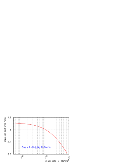
Figure 2: Change of the maximum ion drift time with rate. Calculation using (11).

The Diethorn model has two parameters $\Delta V$ and $K$ which are characteristic for every gas mixture. $\Delta V$ is the potential difference an electron passes between two successive ionisations and $K$ is the critical value of $E/p$ where ionisation starts. $p/p_{0}$ is the ratio of the actual pressure $p$ to the reference pressure $p_{0}$ where K was determined.
For calculating the actual gas gain at rate $R/L$, one now has to replace $V$ by $V-\delta V$ in (10) where $\delta V$ is given by (9). $\delta V$ depends on the gain and vice versa. The two equations have been solved in an iterative way to get a self consistent gain for every rate.
One more correction has to be made for high rates: it was ignored in (3) that the ion drift time $t_{+}$ depends on the rate. For a better approximation of $t_{+}$ in (9), one can insert into (2) the electric field (2) which leads to the formula

$$t_{+}=\frac{p\varepsilon_{0}}{\mu\rho e}\cdot\ln{\left[1+\frac{\rho eb^{2}\ln{\frac{b}{a}}}{2\varepsilon_{0}\left(V-\delta V\right)}\right]}\ .$$ (11)

In the limit of rate $\rightarrow 0$, this is identical to (3). The change of $t_{+}$ with rate is plotted in fig.2 for the gas Ar-CH₄-N₂ 91-5-4 %.

3 Experimental Setup

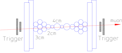
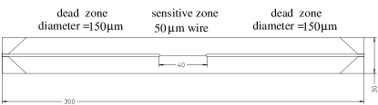
Figure 3: Top: schematic drawing of the chamber, view from top. Bottom: setup of a single tube. The wire is silver coated to avoid gas amplification except for 4 cm in the middle part.

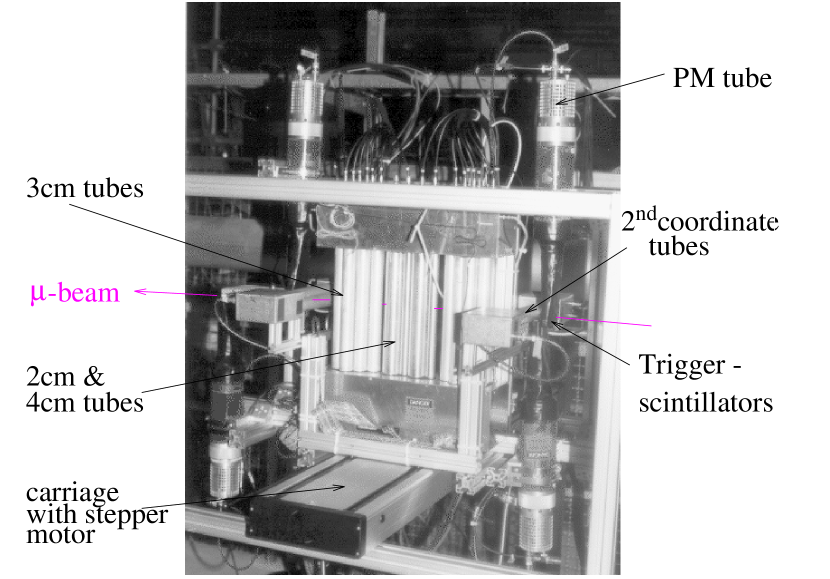
Figure 4: Photo of the apparatus in the 190 GeV muon beam at CERN. One can see two bundles of 8 tubes with 3 cm diameter, two tubes with 2 cm and two tubes with 4 cm diameter. In order to measure the second coordinate, there are two tubes perpendicular to the others at each side of the chamber. The trigger is very small, covering only an area of 1 $\times$ 6 cm² in the sensitive zone of the tubes.

To measure effects of high rates, a specially designed chamber was built for operation in the M2 muon beam at CERN. The task of this setup was to see only effects coming from space charges and to avoid measuring electronic effects such as saturation of preamplifiers, baseline shifts etc. A schematic drawing and a photo are shown in figs. 3 and 4, respectively. The chamber consists of 24 drift tubes: two bundles of eight tubes with 3 cm diameter, two tubes with 2 cm and two tubes with 4 cm diameter. The tubes are glued together precisely, and the two bundles are staggered to improve track fitting.
For measuring the second coordinate, four tubes are placed perpendicular to the others. All tubes are 30 cm long, but the active length is only 4 cm in the middle part of the tubes for the precision coordinate and 10 cm for the second coordinate (fig. 3 bottom). In order to passivate the rest of the tube, the wires have been coated galvanically with silver to increase the wire diameter from 50 $\mu$m to 150 $\mu$m in order to avoid gas amplification. The trigger is made of a coincidence of four scintillation counters which cover an area of 1 cm (along the wires) $\times$ 6 cm (= two tubes in height) and are placed in the middle of the active part of the tubes.
The whole setup can be moved horizontally by a stepper motor within a range of 1 m from the centre of the muon beam. By moving the apparatus with respect to the beam one can adjust the trigger rate from 10 Hz/cm² up to more than 10 kHz/cm².

4 Data Readout and Analysis

Whereas in Atlas the tubes will be read out with TDCs, here the full analog pulse information was read out with 250 MHz flash ADCs [5]. This is necessary for measuring pulse height reductions and to be independent of a fixed discriminator threshold.

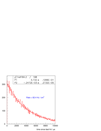
Figure 5: Time differences between two hits in a tube. Fitted to the data is an exponential function $f(t)=\exp{\left(p_{1}+p_{2}t\right)}$.

An important property of the data acquisition was the ability to record at least 8 successive tracks without dead time. This is necessary for the calculation of time distances between consecutive hits from which the particle rate is calculated. It is also used to observe effects coming from event-to-event fluctuations where the ”history” of the tube has to be known. Thus it can be studied how previous hits influence the properties of the detector for the following hits.
In order to achieve this readout without dead time, a trigger logic has been set up that does not need any readout cycle between the first and eighth event trigger. The memory depth of the flash ADC is 2048 bytes per channel corresponding to 8192 ns in time which is large enough to store the waveforms of 8 pulses. The digitization of the flash ADCs is started for each new muon trigger and stopped after 1 $\mu$s.

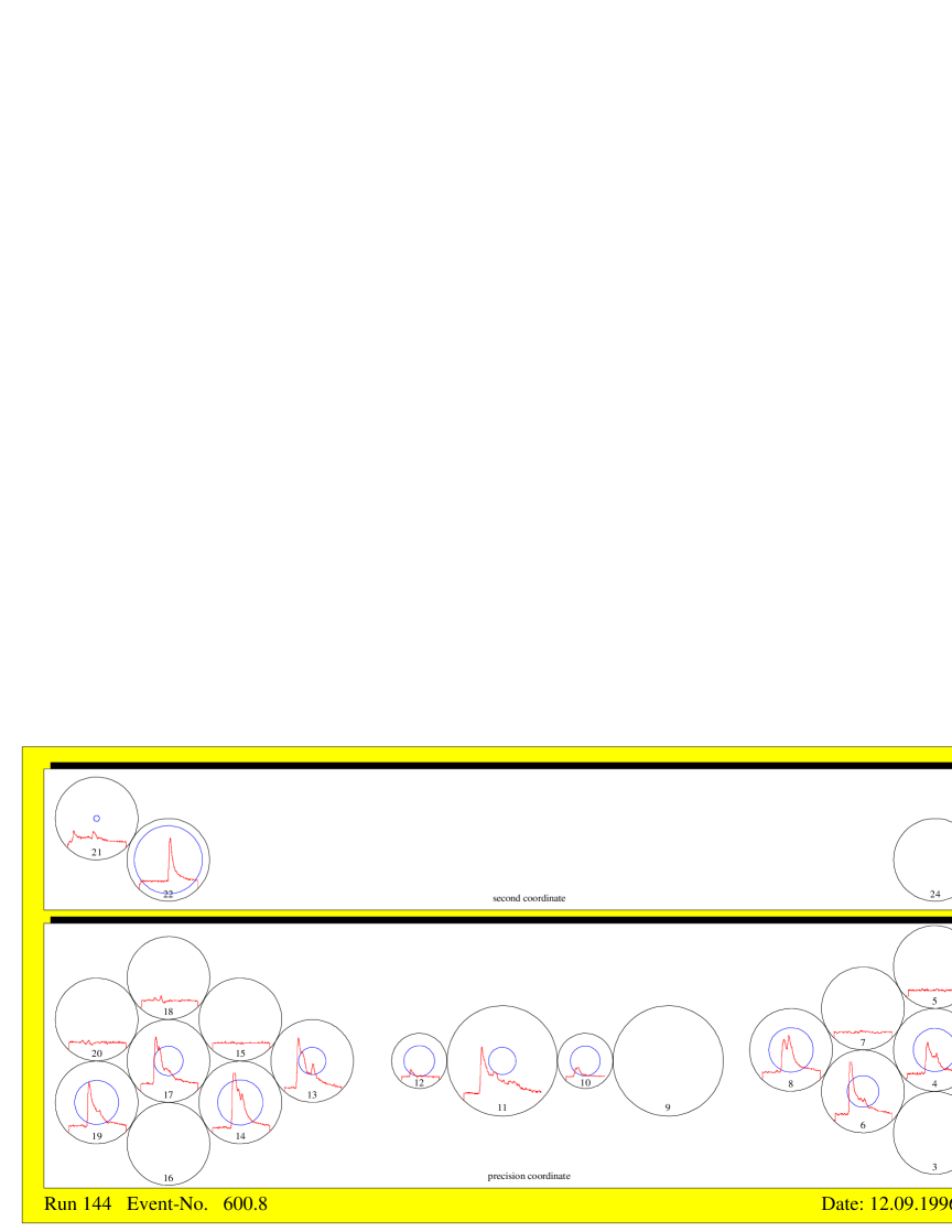
Figure 6: Event display of a muon traversing the chamber. The upper part shows the second coordinate tubes. A circle inside a tube indicates the reconstructed drift distance if a pulse was found. The empty tubes have not been read out.

The time differences between consecutive triggers were measured with a setup of slow TDCs (5 MHz clock) covering a time range of $\approx$ 20 ms. With this information it is possible to compute for every tube the time differences to the last hit. The distribution of these times is exponential (fig. 5). The mean value is $\langle t\rangle=\frac{-1}{p_{2}}$, in agreement with the number of triggers per second counted with a scaler. With this measurements we know both, the time difference between two consecutive hits and (from the second coordinate measurements) the spatial distance of the muon tracks along the wire.
A typical size for the data that had to be read out after every cycle (8 events) was 40 kB. The data were processed by a VME processor operated under OS 9 and stored on an exabyte tape. To maximize the readout speed, all time critical routines have been written in assembler code. The maximum readout rate that could be achieved (if the particle rate was high enough) was $\approx 800$ events within one spill of the CERN SPS accelerator (2.4 s beam followed by a pause of 12 s) and was limited by the speed of the tape drive. The time needed to take a high statistics run (800.000 triggers) at highest rates was 4 hours.
A slow control system was installed to monitor the relevant parameters such as temperature, gas flow, gas mixture, pressure and the high voltages of the tubes.
The measurement of drift times with this kind of flash ADC needs a special setup. The time difference between incoming start signal and start of the digitization can vary randomly between 0 and 12 ns. In order to get a precise time marker, the trigger signal starting the readout was delayed by 800 ns and fed into the test input of the preamplifiers FBPANIK-04 [6]. Thus, every drift chamber pulse was followed by a reference pulse coming always with the same delay with respect to the muon trigger. The time difference between the pulse and the reference pulse is the drift time plus a constant offset t₀.
The time bins of the flash ADCs have a width of 4 ns. To get a better time resolution of the pulse, the DOS (difference of samples) method was used which was developed for the analysis of the flash ADC data of the OPAL experiment[7, 8]. This method is numerically rather simple but very efficient in both finding pulses and calculating the drift time with an accuracy better than 1 ns. First, the pulse shape is differentiated by subtracting the pulse heights of successive bins. Then pulses can be found if the differentiated pulse reaches a certain threshold. Finally the drift time is calculated as the weighted mean of the differentiated pulse around the position of the maximum of the differentiated pulse.
An event display of a muon passing the chamber is shown in fig. 6.

5 Gain Reductions

In order to measure the correct gain drop that is only due to particle rate one has to take care of several effects that influence the measured pulse height. First of all, only data from the same tube are compared to exclude systematic errors like dependence on preamplifiers or slightly different gas mixtures.
One important quantity is the temperature of the gas. The pulse height increases with temperature if the pressure is kept constant (fig. 7). The order of magnitude of this effect is some percent per Kelvin.

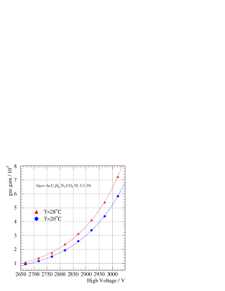
Figure 7: Measurements of the gas gain for Ar-C₂H₆-N₂-CO₂ 92-3-2-3 %. For precise measurements of the gain it is necessary to keep the temperature constant. The solid lines show the Diethorn fits to the data taken at 20^oC and 28^oC.

Figure 8: The pulse height depends on the drift distance. This is due to the different pulse shapes for pulses with short and long drift distances. Measurement with Ar-CH₄-N₂ 91-5-4 % at 3 bar and a gas gain of $2\cdot 10^{4}$.

Figure 9: Histogram of the maximum pulse heights of measured pulses. A Landau function is fitted to this distribution to determine the most probable pulse height.

Since the data were taken in a non-air-conditioned hall with temperature variations of up to 5 K within one measurement, temperature corrections of the pulse height had to be done. Gas gain measurements at different temperatures have been done with the setup described in [9] for the gases that were tested in beam measurements. Thus it was possible to apply the correct temperature corrections and to get the Diethorn parameters needed for the calculation.
However, the most important point is to compare only pulses with equal drift times for the primary electrons. As can be seen in fig. 8, the measured pulse height increases with drift time (with distance from the wire). Pulses with a short drift time have a lower maximum and a longer tail compared to those with long drift time – although the primary ionisation is lower due to the shorter track length inside the tube. Therefore, a cut on the drift time was applied to ensure that only pulses with approximately the same drift distance were compared.

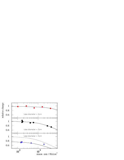
Figure 10: Left: Degradation of the gain with rate. Right: gain reduction vs rate for 2, 3 and 4 cm tubes. The relative charge 1 refers to the charge deposit for a muon track in a 3 cm tube operated at a gas gain of $2\cdot 10^{4}$. The markers show measured data, the lines are calculations. The dashed line in the right plot is an extraplolation from the measured data to rel. charge=1. All measurements were done with the gas Ar-C₂H₆-N₂-CO₂ 92-3-2-3 %.

After these cuts, the maximum of each pulse was determined and histogramed. Because the muons are minimum ionising particles, the distribution of the pulse heights follows a Landau function [10] which was fitted to the data. This is shown in fig. 9. To describe the distribution of the pulse heights, the most probable pulse height (which is one parameter of the fit) was used and not the mean value of the data sample (which is bigger). In the following pulse height means the most probable pulse height of the Landau fit.
Fig. 10 shows the behaviour of the pulse height with increasing rate for three different settings of the high voltage, corresponding to gas gains of $1.5\cdot 10^{4}$, $2\cdot 10^{4}$ and $4.5\cdot 10^{4}$ at zero rate.
The solid lines show a calculation of the pulse height using the Diethorn formula (10) to calculate the gain drop. For the calculation of the electric field (2) and the actual gain, several iterations of the calculation of $\delta$V (9), the gas gain (10) and the maximum ion drift time (11) are necessary to obtain an accurate value for the charge density $\rho$ (4). To compare measured pulse height and calculated gain, one needs to know the ion mobility which was fitted to $\mu=1.5\,\frac{cm^{2}bar}{Vs}$ and found to be consistent with the value of 1.53 $\frac{cm^{2}bar}{Vs}$ for Ar⁺ in Ar from [11, 12].
One can see that an initially high gas gain drops rather fast with increasing rate, going down to 30% of its initial value at 10 kHz/cm². For nominal Atlas conditions with a gas gain of 2$\cdot 10^{4}$ and photon rates $\leq$ 100 Hz/cm² (corresponding to a muon rate of 200 Hz/cm²) the behaviour is rather uncritical, the reduction is some 10%.
However, at very high rates, the pulse height is rather independent of the high voltage, the electric field is reduced to the same limiting value. The order of magnitude of the gain drop with rate is approximately the same for different gases, but the gain drop is larger for gases with low working point (low high voltage for the same gas gain). In that case, the ion drift time is longer and so the space charge density is higher.
The same study was done for the 2 cm and 4 cm tubes. Because the primary ionisation of a muon is proportional to its path length inside the tube, the signals of a 4 cm tube are higher than those of 3 cm and 2 cm tubes if all are operated at the same gas gain. In order to compare the behaviour of the different tubes, measurements at the same charge per track (not at the same gas gain) at zero rate were compared. For easier comparison, the charge for a 3 cm tube at a gas gain of $2\cdot 10^{4}$ is set to 1 in fig. 10. For the 4 cm tube, no measurement was available for charge=1, so a calculation is shown (dashed line) together with a measurement for lower charge. One can clearly see that the gain drop is increasing for bigger tubes at the same irradiation. It is almost negligible for the 2 cm tube, but even for the 4 cm one, the gain drop is in the order of 20 % at a muon rate of 1 kHz/cm² and the nominal gas gain.
The gain reduction could be totally compensated by increasing the high voltage by $\delta$V (9) corresponding to the actual rate – assuming that the irradiation is homogeneous along the tube.

6 Changes in the Electron Drift Time

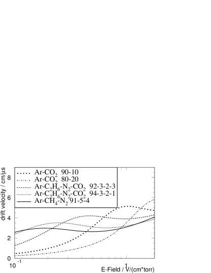
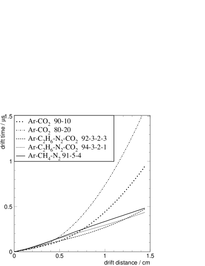
Figure 11: Top: comparison of the drift velocity for different gases. The typical electric field inside a drift tube ranges from 0.15 V/(cm torr) at the tube wall of a 3 cm tube up to 1.8 V/(cm torr) at 1 mm from the wire. Bottom: r-t relations for these gases. Gases with linear r-t relation have a rather constant drift velocity in the relevant region of E/p compared to the other gases.

Figure 12: Fit of the maximum electron drift time. A Fermi function is fitted to the end of the drift time distribution.

The electric field for drifting electrons is changed with rate according to (2). Whereas the field changes are more or less the same for different gases at the same rate (at least if they have to be operated at the same high voltage), the effects to the electron drift times are different. The drift time is given by

$$t(r)=\int_{a}^{r}{\frac{dr^{\prime}}{v(E(r^{\prime}))}}\ \ \ .$$ (12)

The change in drift time depends on the slope of the drift velocity $v(E)$ with the electric field. A gas becomes faster with rate if the slope is positive and slower if it is negative.
One can see here that in order to keep the drift time changes small, one has to look for gases with constant drift velocity, so called linear gases (linear because in this case, the r-t relation is a straight line). Fig. 11 shows the drift velocities and the corresponding r-t relations for the three gases that have been studied in this experiment: the linear gases Ar-CH₄-N₂ 91-5-4 %, and Ar-C₂H₆-N₂-CO₂ 94-3-2-1 % and the rather non-linear Ar-C₂H₆-N₂-CO₂ 92-3-2-3 %. For comparison, the very non-linear gases Ar-CO₂ 80-20 % and Ar-CO₂ 90-10 % are added.
To study the effects of the modified electric field, we look at the change of the maximum electron drift times at different irradiation rates.
The maximum drift time can be calculated using (12) with $r=$ radius of the tube. To do this, one needs to know the drift velocity $v(r)$ of the gas mixture. The Magboltz [15] program was used to calculate the drift velocity as a function of the reduced electric field $v(\frac{E}{p})$. Eq. (2) was taken to calculate the correct electric field $E(r)$ and then the new r-t relation was integrated using (12).
For using the equation (2) the same numbers for the charge density (and the ion mobility) were used as for the calculation of the gain drop in the previous section. The calculated maximum drift time is shown as lines in fig. 13, together with the measured points.
The maximum electron drift time of the measured data can be determined from the falling edge of the distribution of the drift times. Because of diffusion and vanishing ionisation at the tube wall, the tail is smeared. To get a precise and reproducible number, a Fermi function $f(x)=\frac{p_{1}}{exp((x-p_{2})/p_{3})+1}+p_{4}$ has been fitted to the distribution ([13]). The four parameters of the fit are the upper level ($p_{1}$), the time at half height ($p_{2}$), the slope of the fall ($p_{3}$), and an offset ($p_{4}$). Parameter $p_{2}$ is taken as the maximum drift time. The physical maximum drift time may be different from this value by a constant offset. However, we are primarily interested in changes of the maximum drift time. An offset between measurement and calculation was fitted and compensated.

Figure 13: Left: Comparison of measured change in the maximum electron drift time and calculation for different gases (3 cm tubes) Right: Comparison of the change of the maximum drift time versus rate for tubes of 2, 3 and 4 cm diameter. All measurements in the right plot were done with the gas Ar-C₂H₆-N₂-CO₂ 92-3-2-3 %.

Three gases are shown in the left plot of fig. 13 for a 3 cm tube: the linear gas Ar-CH₄-N₂ 91-5-4 %, the non-linear gas with the same maximum drift time Ar-C₂H₆-N₂-CO₂ 92-3-2-3 % and the linear gas Ar-C₂H₆-N₂-CO₂ 94-3-2-1 %. For the first one, the maximum drift time is stable up to very high rates with a tendency to increase with rate. The non-linear one shows already differences of several nanoseconds at rather low rates (100 Hz/cm²). For comparing the 2 cm and the 4 cm tubes to our standard 3 cm one, fig. 13(right) shows the change of the maximum drift time with rate in each case.
The data points for the 3 cm tube are the same as in the left plot for the gas Ar-C₂H₆-N₂-CO₂ 92-3-2-3 %. The solid lines show the calculation done in the same way as for the left plot. The datasets used to compute the right plot are the same as those for the right plot of fig.10.
As for the gain reduction, one can see here that space charges become more and more important if the tube diameter is increased. The 2 cm tube might be operated with a non-linear gas if that was already considered impracticable for a 3 cm tube. For the 4 cm tube, the drift characteristics are dramatically changed at particle rates of 1 kHz/cm² or more. It is surely not advisable to use it for high precision measurements at high rates.
Surprisingly, both measurement and calculation show that the gas with the most linear r-t relation is not the one that is most insensitive to rate. The reason for this is the fact that the operation point of Ar-C₂H₆-N₂-CO₂ 94-3-2-1 % is much lower compared to the others (2575 V instead of 3300 V for Ar-CH₄-N₂ 91-5-4 % and a 3 cm tube. This lower voltage has two effects:

• the amount of space charge is proportional to the inverse of the voltage. $\rho\propto t_{+}\propto\frac{1}{V}$ because of (4) and (3).

• the relative change of the electric field is proportional to the inverse square of the voltage
  

  

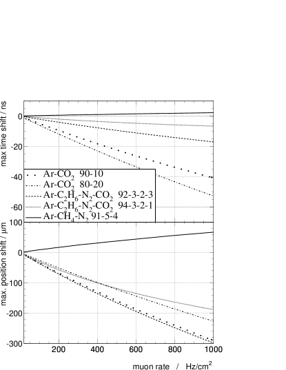
  Figure 14: Top: Change of the maximum drift time with rate. Same calculation as in the previous plot. For comparison, the very non-linear gases Ar-CO₂ 80-20 % and Ar-CO₂ 90-10 % are added. Bottom: corresponding shift in the spatial position.

  

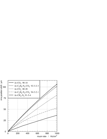
  Figure 15: rms of the position shift for all radii at given rate.

  $\frac{\Delta E}{E}\propto\frac{1}{V^{2}}$ because of (2).

Both points show that an optimum gas should have a high operational voltage. The reason for the rather low working point of this gas is the use of C₂H₆ as quencher. By replacing the Ethane with Methane, the voltage for the same gas gain will increase by 500 V keeping the r-t relation almost unchanged.
Fig. 14 shows the same calculation as fig. 13 for low rates in a linear scale. Additionally, calculations for the gases Ar-CO₂ 80-20 % and 90-10 % are shown for comparison with non-linear gases.
Instead of comparing time shifts it is more adequate to compare the resulting shift in position. Fig. 14 bottom shows this position shift (=the difference between real an assumed position of the particle) when using the r-t relation suited for rate=0 at the actual rate. This value is plotted for the maximum drift radius (1.5 cm) where for most gases this shift has a maximum. It is much smaller for smaller drift radii. The reason for this is the slope of the drift velocity with the electric field (fig. 11). If it is zero, there is no shift because the drift velocity stays constant. If the slope is monotonous the shift increases with drift radius. This is the case for most gases. For the gas Ar-CH₄-N₂ 91-5-4 %, the slope is very low and the sign changes twice in the relevant range of E/p so the integrated effect is almost zero for the maximum drift distance.
Calculating the rms of the values for all radii at given rate leads to fig. 15. This is a good measure for comparing the rate behaviour of different gases. Typical values are in the order of 50-100 $\mu$m for a muon rate of 1 kHz/cm², but for linear gases 30 $\mu$m can be reached which is almost negligible compared to the intrinsic resolution of 70 $\mu$m of the tube.

Figure 16: Difference of the rt relations calculated from data for rates of 150 Hz/cm² and 1200 Hz/cm².

The position shift does not necessarily decrease the resolution of the drift tube. If the rate is stable, one can calculate an adapted r-t relation where the position shift is compensated. Such a r-t relation can be calculated directly from the data with the autocalibration method [16]. Fig. 16 shows the difference between two r-t relations calculated from data at rate=150 Hz/cm² and rate=1200 Hz/cm².

7 Fluctuations

In this section we will show that the resolution becomes worse at high particle rates even if one uses the r-t relation with the position shift compensated. It will be shown that the reason for the resolution loss is the fluctuation of the times between two hits which was ignored up to now where only the mean value was taken into account. Fig. 5 shows that the times between two hits are distributed exponentially. The time constant of the exponential function is defined by the rate. That example for rate $\approx$ 80 Hz/cm² also shows that for roughly half of the events the last hit was more than 4 ms ago, which is the time of the ion drift for a 3 cm tube. In that case, all space charges are gone and the tube behaves as if the rate was zero. On the other hand, we know that for a rate of 80 Hz/cm², the mean position shift is not negligible for most gases. If the time distance between two events is much shorter than 4 ms, one has to take into account all hits within this time window in order to get the correct r-t relation. This is impossible for most applications.
With our setup, it is possible to see the influence of previous hits. Fig. 17 shows how the maximum drift time depends on the time since the last event passed for the gas Ar-C₂H₆-N₂-CO₂ 92-3-2-3 %. All tracks were used that were within one cm along the wire coordinate. A tighter cut did not change the behaviour significantly.
The second example (fig. 18) shows the pulse height versus the distance $\Delta$z along the wire to the previous track. One can clearly see a decrease of the pulse height in the immediate vicinity ($\leq$ 1 mm) of the previous track, but the effect is very small ($<$2%).

Figure 17: Maximum drift time vs time since last hit in the tube (gas=Ar-C₂H₆-N₂-CO₂ 92-3-2-3 %).

Figure 18: Pulse height reduction versus distance along the wire to the previous track (gas=Ar-C₂H₆-N₂-CO₂ 92-3-2-3 %).

For a better understanding of the space charge fluctuations, a simulation study was done and afterwards compared to the measured data. In a first step, it was investigated, how an ion cloud produced at the wire evolves with time in three dimensions. A typical charge cloud consists of 10⁷ ions (primary ion pairs multiplied by gas gain). Ions were generated near the wire with an initial radial coordinate distributed exponentially within 50 $\mu$m from the wire. The position of the coordinate along the wire (z) was distributed like a gaussian with $\sigma_{z}=0.2$ mm. The same was true for the azimuthal angular distribution with $\sigma_{\phi}=60^{\rm o}$. The ions were represented by 1000 points, each one carrying 1/1000 of the total charge. The effective electric field (coming from the applied voltage and the field of the point charges) was calculated at each of these points. Now, one can calculate the drift velocity of the ions and from this the new position after the time dt. To describe the status of the whole cloud at the time T after creation, the mean value and the rms of the coordinates r, $\phi$ and z were calculated.
In the simulation, the extension of an ion cloud does not exceed $\sigma_{z}=0.5$ mm) over the whole drift path. But within a z range of 5 mm, field distortions cause changes in the drift time of more than 1 ns for non-linear gases (e.g. Ar-C₂H₆-N₂-CO₂ 92-3-2-3 %). On the contrary, for the pulse height (or the gain) only the electric field in the immediate vicinity of the wire is relevant. The field distortions coming from an ion cloud that is some mm away are negligible compared to the very high field near the wire.

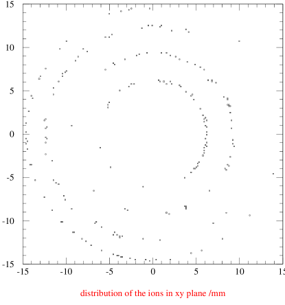
Figure 19: Sample of the distribution of positive ions in the tube. One can see five rings resulting from previous hits.

In a second step of the simulation, the time distances T_i between two hits were generated according to the given rate. Ions were generated at positions according to the results of step one for all previous tracks within the time of the ion drift. Fig 19 gives an example of the distribution of space charges coming from different events. Now, electrons were put at radii r=0.5 mm … r=14.5 mm (or the respective tube radius for the 2 and 4 cm tubes) and the drift in the (static) field resulting of all relevant space charges and the applied voltage was calculated. The time needed to arrive at the wire was histogramed for each radius.

Figure 20: Left: distribution of drift times for radius=14.5 mm for a particle rate of 200 Hz/cm². Right: position shift between real position and the one calculated with the r-t relation. Simulation done for the gas Ar-C₂H₆-N₂-CO₂ 92-3-2-3 %

Fig. 20 (left) shows the distribution of these times for radius= 14.5 mm. The right plot shows the position shift resulting from inserting the drift times in the r-t relation (for rate=0) and subtracting the real position where the electron started. The big, narrow peak belongs to tracks where no charges were inside the tube because the last hit was longer than the ion drift time ago. The distributions become more and more gaussian for higher rates.
From the histogram of the position shifts, two parameters are extracted: the mean value which tells how wrong the r-t relation is for the actual rate and the rms which gives the contribution to resolution decrease. This number has to be added quadratically to the resolution of the drift tube at zero rate to get the correct value for the resolution at the investigated rate.

Figure 21: Simulation of the mean position shift (top) versus radius for different particle rates. Bottom: the contribution to resolution decrease of the tube. The numbers are of the same magnitude for rates up to some 100 Hz/cm², for higher rates, the shift increases faster.

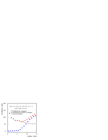
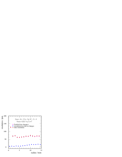
Figure 22: Resolution of the tube. Shown are the curves coming from a Garfield simulation, the simulated contribution coming from space charges and the quadratical sum of both. Top: gas=Ar-C₂H₆-N₂-CO₂ 92-3-2-3 %, bottom: gas = Ar-CH₄-N₂ 91-5-4 %

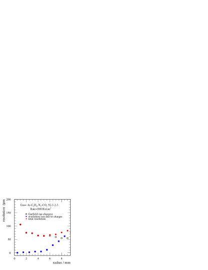
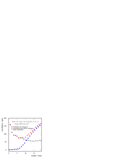
Figure 23: Behaviour of 2 cm (top) and 4 cm tubes (bottom). The corresponding plot for the 3 cm tube is fig. 22(top).

Figure 24: Measured resolution for the gas Ar-C₂H₆-N₂-CO₂ 92-3-2-3 %. For the top plot, all events were taken, for the bottom one only those were selected, where the previous hit was longer than the ion drift time ago.

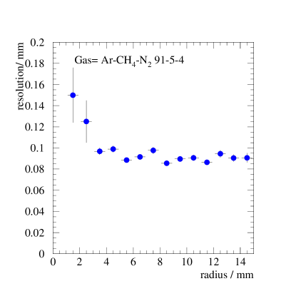
Figure 25: Measured resolution for the gas Ar-CH₄-N₂ 91-5-4 % with no cut on the history of the tube. Rate=450 Hz/cm².

For comparison with the measurements and the analytical calculation done in the previous section, the mean position shifts for rate=0 … 1 kHz/cm² have been calculated (fig. 21, top). They agree within 5% with the values shown in fig. 14 (bottom) for the gas Ar-C₂H₆-N₂-CO₂ 92-3-2-3 %.
Fig. 21 bottom shows the corresponding rms values of the position shift histogram. This is the contribution to the resolution loss coming from fluctuations. The numbers are non-negligible in the case of high rates and for high precision drift tubes like those of the muon spectrometer for Atlas. In that case, the resolution of the tubes is dominated by this effect for a non-linear gas.
Calculations of drift chamber properties can be done very precisely using the Garfield [17] program. It also gives reliable numbers for the expected resolution (at zero rate). It was used to compute the resolution of the gases Ar-C₂H₆-N₂-CO₂ 92-3-2-3 % and Ar-CH₄-N₂ 91-5-4 % with parameters discriminator threshold, noise etc set as expected for Atlas conditions. The result is shown in fig. 22 (open circles). On the contrary to the results shown before, the gas gain was doubled to $4\cdot 10^{4}$ in order to have the same amount of space charges at the same rate as expected for the photons of the Atlas background. Also the measured data that will be shown below refer to muon data with a gas gain of $4\cdot 10^{4}$.
The results of the resolution loss for a rate of 500 Hz/cm² are shown as squares. The total resolution (filled circles) is then given as a quadratical sum of both contributions. For the first gas, space charges play an important part for radii $>$ 8 mm, becoming the dominant contribution. For the second gas, the resolution is not affected by space charges even at very high rates. The different behaviour of the two gases is in agreement with the expectations: fig. 13 already showed that the drift time is nearly uneffected due to space charges for Ar-CH₄-N₂ 91-5-4 %. For this linear gas, the drift velocity stays constant with changing electric field - in contrast to the non-linear gas.
An experimental proof of these simulations is shown in figs. 24, 25. Tracks have been fitted through the chamber and the resolution of a single tube was calculated for different conditions. For the gas Ar-C₂H₆-N₂-CO₂ 92-3-2-3 %, one can see in both, measurement and simulation a degradation of the resolution for big radii in the case of high rates. It is not visible if one takes only low rate data or – as in shown in fig. 24(bottom) – selects from a high rate run only those events where the previous track was longer than the ion drift time ago and all space charges are gone.
The degradation of the resolution is also not visible for a linear gas (fig. 25) where data were taken at the same rate and no cut on the event selection was applied.
The measured resolution is slightly worse (also for low rate) than the simulation. This is due to the higher noise and a higher threshold for identification of the pulses needed for our flash ADCs. The simulation shown refers to TDC measurements as foreseen for Atlas. Increasing the relevant parameters brings the simulation in accordance with our measurements.
Finally, the expected resolution of 2, 3, and 4 cm tubes shall be compared using a non-linear gas (for a linear one, the differences are mostly negligible in all cases). The 3 cm results are shown in fig. 22, the others in fig. 23. The 2 cm tube is nearly unaffected by the high irradiation, a resolution loss occurs only in the last 2 mm. On the contrary, for a 4 cm tube the resolution is dominated by the space charge contribution and the mean spatial resolution becomes much worse than 100 $\mu$m.

8 Conclusion

Gain reduction and changes of drift times have been measured as a function of the rate. For the gases that have been tested, a good agreement between measurements and calculation was found. Predictions of the high rate behaviour for new gases can be made without performing measurements.
The gas gain reduction due to space charges is similar for most gases and unavoidable. For a constant rate it could be compensated by increasing the high voltage.
The electric field for drifting electrons is increased because of space charges for radii larger than 4 mm (in a 3 cm tube). For linear gases (like Ar-CH₄-N₂ 91-5-4 %) this may have almost no effect on the r-t relation even at very high rates. For non-linear ones there are already big effects at rates of 100 Hz/cm². Whereas the r-t relation can be adapted for a given irradiation rate, it is (for practical applications) impossible to correct for the field fluctuations resulting from the random distribution of the times between two hits. This gives a contribution to the total resolution of the drift tube which for non-linear gases becomes the dominant limitation of the spatial resolution at large distances from the wire.

References

- [1] R.W. Hendricks, The Review of Scientific Instruments 40, 1216 (1969)
- [2] E. Mathieson, Nucl. Instr. and Meth. A249 (1986) 413
- [3] The ATLAS Collaboration Muon Spectrometer Technical Design Report CERN/LHCC/97-22 (1997)
- [4] W. Diethorn, A Methane Proportional Counter System for Natural Radiocarbon Measurements , U. S. AEC Rep. NYO-6628 (1956)
- [5] B. Struck Tangstedt/Hamburg Technical Manual DL 515 Flash ADC VME Module
- [6] Schematics and Layout: F/B-Muonchamber Pre Amp FBPANIK-04, NIKHEF 1996
- [7] D. Schaile, O. Schaile and J. Schwarz, Nucl. Instr. and Meth. A242 (1986) 247
- [8] S.M. Tkaczyk et al., Nucl. Instr. and Meth. A270 (1988) 373
- [9] K. Handrich Aufbau einer Apparatur und Messung der Gasverstärkung in den Driftröhren des Atlas-Myondetektors,Thesis, University Freiburg 1998
- [10] F. Sauli Principles of Operation of Multiwire Proportional and Drift Chambers, CERN 77-09 (1977)
- [11] E.W. McDaniel and E.A. Mason, The Mobility and Diffusion of Ions in Gases, Wiley, New York (1973)
- [12] Landolt-Boernstein, vol 4/3 Eigenschaften des Plasmas, 6. ed., Springer (1957)
- [13] A. Biscossa et al., ATLAS Internal Note MUON-NO 196 (1997)
- [14] G. Schultz, G. Charpak and F. Sauli, Rev. Phys. Appl.(France) 12, 67 (1977)
- [15] S.F. Biagi, Nucl. Instr. and Meth. A283 (1989) 716
- [16] C. Bacci et al. ATLAS Internal Note MUON-NO 135 (1997)
- [17] Rob Veenhof, Garfield Users Manual, CERN Program Library W5050