The Concurrent Track Evolution Algorithm:

Extension for Track Finding in the Inhomogeneous

Magnetic Field of the HERA-B Spectrometer

Rainer Mankel 

Institut für Physik, Humboldt Universität zu Berlin

Invalidenstr 110, D–10115 Berlin, Germany

and

Alexander Spiridonov 

DESY Zeuthen

Platanenallee 6, D–15738 Zeuthen, Germany

Abstract

The Concurrent Track Evolution method, which was introduced in a previous paper [1], has been further explored by applying it to the propagation of track candidates into an inhomogeneous magnetic field volume equipped with tracking detectors, as is typical for forward B spectrometers like HERA-B or LHCb. Compared to the field-free case, the method was extended to three-dimensional propagation, with special measures necessary to achieve fast transport in the presence of a fast-varying magnetic field. The performance of the method is tested on HERA-B Monte Carlo events with full detector simulation and a realistic spectrometer geometry.

1 Introduction

Dedicated B physics experiments for hadronic interactions, as HERA-B [2] and LHCb [3] are designed as forward spectrometers because of the kinematics of the $b$ hadrons, whose decay particles are produced with a large Lorentz boost. Even with highly granular tracking devices, as honeycomb drift chambers and strip detectors, the large track density leads to high cell occupancies, which can range up to 20% in the “hottest” parts of the HERA-B outer tracker. Under these circumstances, pattern recognition becomes a crucial issue.

In a previous paper [1], the Concurrent Track Evolution strategy has been presented as a method of track finding in a multi-planar tracker geometry. Concurrent Track Evolution is a track following method based on the Kalman filter [4, 5, 6, 7], which evaluates the available paths for a track candidate concurrently to find the optimal solution, but also keeps the combinatorics at a reasonable level (see [1] for details). The method has been successfully applied to find initial track segments in the geometry of the HERA-B pattern tracker, which consists of four superlayers of inner and outer tracking devices in the field-free region between the magnet and the RICH. The layout of the HERA-B spectrometer is shown in fig. 1. A more detailed explanation of the HERA-B tracker and the reconstruction strategy can be found in [1].

The next step in the HERA-B track reconstruction is the track propagation through the magnetic field. Typical sizes of the magnetic field components $B_{x}$, $B_{y}$ and $B_{z}$ as a function of $z$ are displayed in fig. 2. The main bending component ($B_{y}$) has a bell-shaped dependence on $z$, and there is clearly no significant subset of the magnet tracking system in which the field can be regarded as homogeneous. Moreover, the $x$ and $z$ components are sizeable, making it impossible to restrict pattern recognition to projections while making full use of the track model. The necessity to deal with five track parameters simultaneously, and the additional hits generated by spiralling particles make standalone track finding within the magnet a problematic task. Instead, the HERA-B track reconstruction concept operates by first finding straight-line track segments in the pattern tracker (described in [1]) and then propagating them upstream through the magnet area. In a subsequent step, these track candidates will have to be matched to the track segments in the silicon vertex detector. A considerable fraction of the $K^{0}_{S}$ from the golden decay mode $B^{0}\rightarrow J/\psi K^{0}_{S}$ decays too late to produce a sufficient number of hits in the acceptance of the vertex detector, so that the vertex must be reconstructed from the main tracker information.

Compared to pattern recognition from scratch in the magnet, this propagation approach has the advantage that only one track parameter, the momentum, is poorly known and must be fitted during the propagation. There are however several challenges involved:

• Due to the non-linear nature of the fit, iteration, in general, may be required to obtain the optimal result. In particular, it might happen that upstream hits are not found within the predicted error margin because a wrong initial momentum value in the downstream section caused derivatives to be taken at the wrong positions in parameter space. Iteration of the various track candidates in the context of Concurrent Track Evolution, on the other hand, would multiply the computational effort to a worrisome degree.

• The inhomogeneity of the field necessitates a much more costly, numerical transport of the track parameters than in the field-free case. The Kalman filter requires also the transport of the covariance matrices, for which the derivative matrices of the transported versus the original parameters must be calculated.

• The different superlayer structures of outer and inner magnet tracker represent additional challenges to the navigation concept.

2 Geometry

As an example, we will use the current HERA-B detector layout as it is presently implemented in the geometry definition of the experiment. This layout is shown in fig. 1. On the right-hand side, four superlayers of inner and outer tracking devices form the pattern tracker, which is used for finding the initial straight-line track segments. The left part shows the magnet tracker through which these segments have to be propagated. The magnet tracker consists of eight superlayers of outer (MC01...MC08) and four superlayers of inner tracker (MS01, MS03, MS05, MS07). The outer tracker is based on honeycomb drift chamber technology with $5$ and 10 mm diameters, with an assumed resolution of $200\mu$m (see [1, 8] for further details). Each outer tracker superlayer in the magnet consists of three tracking layers with the orientations $+\alpha$, 0^∘, $-\alpha$ with a stereo angle of $\alpha\approx 100$ mrad, except for MC01 which has four layers in a 0^∘, $-\alpha$, 0^∘, $+\alpha$ arrangement to satisfy requirements of second level triggering, and MC05 which consists only of a single 0^∘ layer because of space restrictions inside the magnet yoke. The inner tracker is built of micro-strip gaseous chambers (MSGC) with a typical resolution of $80\mu$m. Each superlayer consists of one zero degree and one stereo layer with a stereo angle of $+100$ or $-100$ mrad, alternatingly, except for MS01 which has four layers with the sequence 0^∘, $-\alpha$, $+\alpha$, 0^∘. The sector structure of the magnet tracker superlayers is similar to that of the pattern tracker (see [1]).

Compared to the setup shown in [1], the stations MC09 and MS09 have been removed because they are already in an area of weak magnetic field and are not expected to improve the track parameters already measured by the pattern tracker significantly. The gaps in the second half of the magnet tracker are reserved for pad chambers designed to generate a pretrigger for high momentum tracks, which is intended to select $B^{0}\rightarrow\pi^{+}\pi^{-}$ decays. In front of MS01, an additional silicon strip detector superlayer is foreseen to cover the innermost angular region. Both the pad chambers and the silicon superlayer were not used in this study.

3 Method

3.1 Seed

A track candidate found in the pattern tracker provides the starting seed, which gives already rather precise estimates of the parameters $x$, $y$, $t_{x}=p_{x}/p_{z}$ and $t_{y}=p_{y}/p_{z}$ at the entrance of the pattern tracker, which is at $z\approx 700$ cm. We use the inverse momentum signed according to charge, $Q/p$, as momentum parameter because it is most convenient to use in the numerical treatment of transport within the magnetic field. Since iterations are to be avoided, it is essential to have already an estimate of the momentum parameter which is good enough to give reliable parameter derivatives. Such an estimate can be obtained from the visible deflection by the magnetic field assuming that the track comes from the target region:

$$\frac{Q}{p}=\frac{\left[x-(z-z_{target})t_{x}\right]\ \sqrt{1+t_{x}^{2}}}{\int B_{y}d\ell\cdot(z_{magnet}-z_{target})\sqrt{1+t_{x}^{2}+t_{y}^{2}}}$$

where $\int B_{y}d\ell$ is the average field integral of the main bending component, $z_{magnet}$ and $z_{target}$ are the $z$ coordinates of magnet center and target and $x$ and $t_{x}$ are the impact parameter and track angle in the bending plane as given at $z$ by the seed. The quality of this estimate for muons and pions from the golden B decay is shown in fig. 3. The estimate gives obviously reliable results in most cases. The relative precision is $\approx 6\%$ in the muon and $\approx 7\%$ in the pion case, in the latter the estimate is slightly diluted by the displacement of the $K^{0}_{S}$ decay vertex which effects the tail in fig. 3d. The initial covariance matrix diagonal element of the momentum parameter is set accordingly.

3.2 Modifications to the Concurrent Track Evolution method

After the initial seed definition from the pattern tracker, the Concurrent Track Evolution mechanism [1] propagates the candidate as far as possible upstream within the magnet tracker, employing the Kalman filter technique. This is achieved by a succession of growth cycles, which explore the possible continuations from layer to layer. A certain number of branches is propagated concurrently to explore the available paths. We summarize here briefly the steps which are explained in detail in [1]:

1. Based on the position of the last hit of a candidate, generate a list of detector plane parts in which the next logical hit is expected, using the domain navigation method described in [1]. Define a search window in each plane, using the Kalman filter prediction from the last hit.

2. Create a new branch for each hit found in each search window.

3. Filter each hit and accept the new branch if the $\chi^{2}$ contribution is not too large.

4. At the end of each growth cycle, locate the best candidate according to a quality estimator function. Discard all branches whose quality estimates differ by more than a given maximum value, keep only the ${\cal R}_{max}$ best candidates.

5. Repeat the steps above, until no further growth is possible. This may be either because the end of the tracking system is reached, or because no further suitable hits are found.

6. Select the best remaining candidate, and store it if its hit count exceeds a certain minimum.

Compared to the algorithm decribed in [1], the following changes and extensions have been made:

1. The algorithm is applied in three dimensions. The same navigation strategy as in [1] is used, but a domain window is immediately discarded if it is not intersected by the extrapolated track candidate.

2. Hits are considered for filtering if they are within either three standard deviations or 2 cm of the predicted projected coordinate $u=x\ \cos\alpha_{st}-y\ \sin\alpha_{st}$ (where $\alpha_{st}$ is the stereo angle).

3. After filtering, the new candidate is accepted if the $\chi^{2}$ contribution is less than 16.

4. In the quality estimator $Q$ (see [1]), which is calculated from the number of hits and their $\chi^{2}$ contributions, the weight of the latter ($w_{\chi^{2}}$) is set to 0.05.

5. If at least one new track candidate is obtained through successful continuation, its parent track candidate is excluded from further propagation, This is unlike the strategy in the projection-based tracking in [1]: without knowledge of the orthogonal coordinate, the probability to pick up a wrong hit within the prediction window was higher, so that the possibility of a missing hit (fault) had to be considered even if a continuation hit had been found.

6. Since the magnet part of the inner tracker has only about half as many layers as the outer tracker, the inner tracker hits are weighted by a factor of two when the number of hits is calculated. A track is accepted for storage if its weighted number of hits, acquired in the magnet tracker is at least 5.

The maximum number of missing hits in sequence ($N^{max}_{Faults}$) is kept at 2, and the maximum number of track candidates treated concurrently (${\cal R}_{max}$) remains at 5.

3.3 Transport of track parameters within the magnetic field

Compared to the field-free case discussed in [1], where two-parameter states are transported linearly, the transport within the inhomogeneous field is much more critical because there are five track parameters involved, and both the parameters and their covariance matrix must be transported. Regarding the number of track candidates which appear in the course of Concurrent Track Evolution, very efficent numerical procedures are needed in order not to exceed practical cpu time limitations.

It has already been shown that the precision requirements of HERA-B tracking can be met using a fifth-order Runge-Kutta method with adaptive step size control [9], a procedure which has also been successfully used for track fitting [10]. For the track propagation problem discussed in this paper, we have applied the following flexible strategy (described in detail in [11]) to keep the computational effort at a minimum:

short distances:

for $\delta z<$20 cm, a parabolic expansion of the trajectory, based on the field vector at the starting point, has been used.

medium distances:

for 20 cm$<\delta z<$60 cm, a classical fourth-order Runge-Kutta method [12] has been applied.

long distances:

for $\delta z>$60 cm, a fifth-order Runge-Kutta method with adaptive step size control [12] has been employed.

Since the precision for the derivatives of the transported parameters ($\tilde{x}$, $\tilde{y}$, $\tilde{t}_{x}$, $\tilde{t}_{y}$, $Q/\tilde{p}$) with respect to the untransported ones ($x$, $y$, $t_{x}$, $t_{y}$, $Q/p$) is less critical than the precision of the parameters themselves, the sizes of the derivatives were studied and their influence on the track finding result was carefully investigated [11]. It was found that the derivatives with respect to the first four parameters can be approximated by

$$\partial(\tilde{x},\tilde{y},\tilde{t}_{x},\tilde{t}_{y},Q/\tilde{p})/\partial x=(1,0,0,0,0)$$

$$\partial(\tilde{x},\tilde{y},\tilde{t}_{x},\tilde{t}_{y},Q/\tilde{p})/\partial y=(0,1,0,0,0)$$

$$\partial(\tilde{x},\tilde{y},\tilde{t}_{x},\tilde{t}_{y},Q/\tilde{p})/\partial t_{x}=(\tilde{z}-z,0,1,0,0)$$

$$\partial(\tilde{x},\tilde{y},\tilde{t}_{x},\tilde{t}_{y},Q/\tilde{p})/\partial t_{y}=(0,\tilde{z}-z,0,1,0)$$

without loss in efficiency but with large gain in speed. The derivatives with respect to the momentum parameter are approximated as

$$\partial(\tilde{x},\tilde{y},\tilde{t}_{x},\tilde{t}_{y},Q/\tilde{p})/\partial(Q/p)=(\partial\tilde{x}/\partial(Q/p),0,\partial\tilde{t}_{x}/\partial(Q/p),0,1)$$

where $\partial\tilde{x}/\partial(Q/p)$ and $\partial\tilde{t}_{x}/\partial(Q/p)$ are defined by differential equations which are solved together with the integration of the equations of motion by the Runge-Kutta method.

These approximations lead to a derivative matrix whose elements contain mainly ones and zeroes. This property is used to reduce strongly the number of computations for the transport of the covariance matrix.

The propagation of electrons and positrons within the magnetic field is complicated by the energy loss through bremsstrahlung. An additional radiative energy loss correction according to the method of Stampfer et al. [13, 7] has been applied, which was found to improve the magnet tracking efficiency for electrons from the golden $B$ decay by 0.5% with respect to the number of reference tracks (sec. 4.2).

4 Performance

4.1 Event sample

Samples of 1219 interactions of the type $pAl\rightarrow B^{0}+X$, $B^{0}\rightarrow J/\psi K^{0}_{S}\rightarrow(\ell^{+}\ell^{-})(\pi^{+}\pi^{-})$, with 915 decays into the muon and 304 into the electron channel, and 2000 unbiased inelastic $pAl$ interactions were generated [14] and passed through the full HERA-B detector simulation [15] to investigate the performance. Both the event generation and the detector digitization were done in the same manner as described in [1].

4.2 Performance estimators

As in [1], efficiencies are calculated for reference tracks which are a track class defined by both the geometrical acceptance and the physics interest of the experiment. Since a track segment from the pattern tracker is needed as a starting point, a magnet reference track has to satisfy all criteria for a reference track in the pattern tracker [1], including the momentum requirement $p>1$ GeV/c. In addition, the track is required to pass at least four layers within the area of high magnetic field, defined by a circle of 140 cm radius around the magnet center in the bending plane. It is also demanded that the track pass at least one layer in the first half of the magnet ($z<450$ cm), to reject late decays where the particles do not traverse a sufficient amount of integrated field. Since it can happen that particles at the outer and inner borders of the acceptance “circumvent” some superlayers, tracks with such gaps are also regarded as not being covered by the geometrical acceptance. Finally, tracks are not considered as belonging to the reference set if they have lost more than 30% of their energy within the magnet. This requirement is directed against radiating electrons which have a reduced probability to be selected by the first level trigger.

A track candidate is regarded to properly reconstruct a particle if at least 70% of its hits were caused by this particle. In addition, it is checked that the first reconstructed hit of the candidate is not further than 100 cm downstream of the first hit of the real particle. The efficiency is then simply the fraction of reference tracks which are successfully reconstructed. In order to isolate the effect of the magnet propagation, we define in addition a magnet pattern recognition efficiency which is defined relative to the track finding efficiency in the pattern tracker:

$$\epsilon_{magnet}=\frac{\epsilon_{magnet+pattern\ tracker}}{\epsilon_{pattern\ tracker}}$$

The efficiency $\epsilon_{pattern\ tracker}$ has been re-evaluated for the geometry and simulated data sample used here and was found to agree, within statistical errors, with the numbers presented in [1].

4.3 Geometrical acceptance

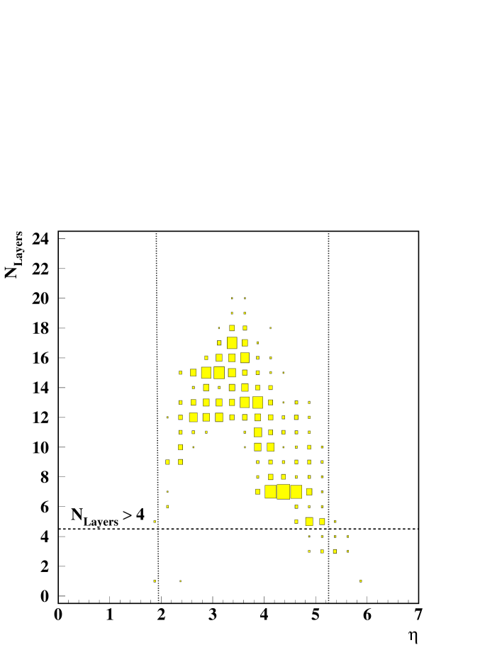
Figure 4: Number of layers passed in the magnet as a function of pseudorapidity $\eta$. The different levels of layer count around $\eta=3$ and $\eta=4.5$ reflect the different number of superlayers of the outer and inner tracking systems. The vertical lines correspond to the nominal acceptance region as described in the text.

In order to verify the adequateness of the reference track criteria, fig. 4 shows the number of layers passed in the magnet, as defined in the last section, as a function of pseudorapidity $\eta$ for muons from the golden B decay which are reference tracks in the pattern tracker. In the outer tracker dominated regime around $\eta=3$, the layer count is higher than in the region governed by the inner tracker around $\eta=4.5$. Obviously the cut $N_{Layers}>4$ gives a generous description of the geometrical acceptance. The nominal rapidity coverage [8], corresponding to 10 mrad at the inner and 250 mrad (horizontal) resp. 160 mrad (vertical) at the outer border, is displayed as a pair of vertical lines in fig. 4.

The fraction of particles which are selected as reference tracks can be interpreted as the geometrical acceptance of the combined system of pattern and magnet tracker. Table 1 summarizes these values for particles related to the golden B decay. Comparison of the muon acceptance of 80.2% with the one of the pattern tracker alone [1] shows that 92% of the muons within the pattern tracker acceptance have also enough hits in the magnet tracker. The electron acceptance is smaller (66.6%) because of the cut on the radiated energy. The pion and $K^{0}_{S}$ acceptances are mainly limited by the $K^{0}_{S}$ decay length which causes a considerable fraction of kaons to decay too late for a good momentum measurement of the pions. The total fraction of golden $B^{0}$ decays with reconstructable condition is 34% in the muon and 29% in the electron channel.

4.4 Efficiency

Figure 5 shows displays of an event with seven superimposed interactions with focus on the magnet tracker region. The Monte Carlo tracks have been drawn by connecting the impact points in the sensitive detector parts, note that because of this technique, low-momentum particles have a poor representation. The region of highest magnetic field which is used for the definiton of reference tracks is shown as a filled circle. While several softer particles are not reconstructed because they do not reach the pattern tracker, the vast majority of tracks passing the full spectrometer is found in full length up to the entrance of the magnet tracker. The second display (fig. 5b) is restricted to the particles from the golden $B$ decay and shows the proper recognition of these tracks.

The pattern recognition efficiencies obtained in B interactions with on average four superimposed inelastic interactions are summarized in tab. 2. The right column gives the relative efficiency of the magnet propagation step. For charged particles from the golden B decay, these efficiencies are larger than 97%. The $\pi^{\pm}$ appears to have a slightly lower efficiency than the leptons which may be attributed to the late decays of some $K^{0}_{S}$’s and the resulting smaller number of hits, and the on average smaller momentum. Charged particles above 1 GeV/c have a magnet propagation efficiency of $\approx 94\%$.

The left column shows the efficiency of the combined pattern and magnet tracker reconstruction. The ratio to the numbers in the right column corresponds within statistical errors to the numbers given in [1]. It is interesting to note that, after the requirement that reference tracks should not radiate more than 30% of their energy within the magnet, electrons and muons have similar efficiencies. The relative rate of ghosts is 2%, corresponding to an average of 0.85 ghost tracks per event. This is much smaller than the 4.4 ghosts per event which remained after pattern tracker analysis [1], which shows the ghost rejection power of the magnet tracker. Further suppression of ghosts is expected from the matching with the vertex detector system.

If one includes the geometrical acceptance, the total fraction of reconstructed golden B decays is 28% in the muon and 24% in the electron channel.

In order to probe the robustness of the algorithm, the efficiency of the magnet tracker propagation step has been studied as a function of the number of superimposed inelastic interactions. Figure 6 shows that the magnet tracking efficiency remains at the same high level up to ten superimposed interactions, so that the total efficiency is governed by the behaviour from the pattern tracker. The ghost rate increases in a well-controlled way.

In order to investigate further the causes for particle loss, we have broken down the magnet efficiency as a function of momentum for muons and pions from the golden B decay (fig. 7). For both particle species, the efficiency saturates on a high level above 5 GeV/c, below this value the efficiency drops, which is likely to be due to multiple scattering effects, or to strongly curved trajectories which are not entirely covered by the navigation tables. At the bottom of fig. 7, it is indicated how the different parts of the momentum range contribute to the mean inefficiency, $1-\epsilon_{Magnet}$. While muons and pions show the same efficiency at a given momentum, the pions suffer more strongly from the reduced efficiency at lower momentum because of their softer spectrum.

Figure 8 shows a similar distribution as a function of the polar angle, measured at the track point of lowest $z$ within the magnet tracker. The magnet track finding efficiency decreases visibly with increasing angle. Since, however, polar angle and total momentum are strongly correlated within the HERA-B kinematics, the effect is not independent from the one in fig. 7.

4.5 Parameter estimates

The underlying reconstruction concept [1] foresees that the track candidates emerging from the magnet track reconstruction should be matched with track candidates found in the vertex detector, or continued into the latter by direct propagation, which is only possible if the track parameters are well estimated. In principle, a fully iterative refit of the trajectory to the hits found by pattern recognition, which takes also additional traversed material into account, can be used to optimize the parameter estimate. Such a fit, the method of which is described in [10], has been used in the following for comparison. From the aspect of cpu time consumption, it would however be preferred if a global refit can be postponed until the hits from all components have been collected.

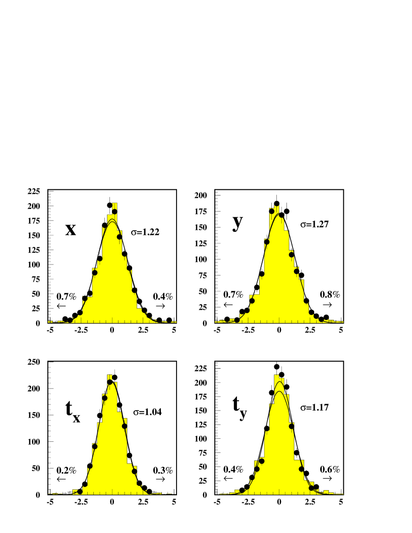
Figure 9: Normalized residuals (see text for explanation) for the parameters $x$, $y$, $t_{x}$ and $t_{y}$ for muons from the golden B decay. The solid points with error bars are directly obtained from the parameters delivered by the magnet propagation, the shaded histogram is the result of an iterative refit which interpolates traversed material between the hits. The result of Gaussian fits to both distributions is also shown, and the standard deviation $\sigma$ is quoted for the refitted case. The percentages at the arrows in the lower parts of the figures give the number of entries below and above five estimated standard deviations for the parameters delivered by the refit.

Figure 9 shows the normalized residuals

$$\frac{{\cal X}_{i}^{REC}-{\cal X}_{i}^{MC}}{{\cal C}_{ii}^{1/2}}$$

where ${\cal X}_{i}^{REC}$ is the reconstructed parameter at the point of lowest $z$ of a track candidate, ${\cal X}_{i}^{MC}$ the corresponding Monte Carlo-truth and ${\cal C}_{ii}$ the estimate for the corresponding covariance matrix diagonal element, where the parameters are ${\cal X}_{i}=$ $x$, $y$, $t_{x}$ and $t_{y}$. (If several track candidates exist for the same particle, the better one is chosen because it is more likely to be selected in the subsequent matching with the vertex detector.) The error estimate ${\cal C}_{ii}^{1/2}$ which is used to normalize the residual is determined by the coordinate resolution and the multiple scattering effects as they are estimated during magnet propagation, or through the full refit. Dilutions due to wrong hits or left/right assignments in the pattern recognition process are expected to lead to widths larger than one. All observed residual distributions have shapes close to Gaussians. There are hardly any tails, as is also reflected in the underflow and overflow percentages which are given in the diagrams, which shows that the criterion used to label a track as reconstructed (see section 4.2) is adequate. The fitted widths exceed the ideal value by 17–27%, which can be attributed to inevitable pattern recognition effects. Only in the case of the $t_{x}$ parameter the excess is smaller (4%), which is not unexpected because the resolution in this parameter is dominated by multiple scattering. One concludes that the track parameters delivered by the magnet propagation are good enough to be directly used by the matching step without a refit at this stage.

The quality of the momentum parameter estimate influences the matching to the vertex detector segment only if the first point (at lowest $z$) is well within the magnetic field, because otherwise a linear extrapolation should be sufficient. Figure 10 shows in its upper part the normalized residual of the momentum parameter ($Q/p$), which does also show only moderate tails and a width only slightly larger than unity. The bottom part of the same figure displays the distribution of the relative momentum error, $\Delta p/p$. Note that the distribution is not expected to be Gaussian because of the momentum spread and multiple scattering effects. The mean relative resolution obtained by fitting the central part of this distribution is $8.7\cdot 10^{-3}$, which the refit improves slightly to $8.1\cdot 10^{-3}$. To compare these resolutions with the technical limit, the same events were passed through a full iterative refit of the hits selected using Monte Carlo information, where a mean resolution of $7.1\cdot 10^{-3}$ was obtained. The resolutions are summarized in table 3. The comparison thus gives an illustration of the size of dilutions caused by pattern recognition effects, which turn out to be relatively moderate. Further improvement can be expected from

1. a rejection of outliers, based on the $\chi^{2}$ contribution of each hit to the final fit, which can diminish the dilution from wrong hits or left/right assignments.

2. successful matching with vertex detector segments, which should reduce the relative influence of wrong hit information within the magnet.

We conclude that the method studied here gives reasonable parameter estimates in spite of the high track densities.

4.6 Speed

In the magnet case, the issue of computing time is potentially even more critical than in the field-free case because of the costly numerical parameter transport within the magnetic field. The time consumption of the magnet part has been tested by running the reconstruction algorithm with and without magnet propagation step and computing the difference. The typical precision of such measurements is $\approx 20\%$. The resulting behaviour as a function of the number of superimposed interactions in displayed in fig. 11. On an SGI challenge workstation, the computing time in case of on average four superimposed inelastic interactions is about 3.6 s. The increase with the number of interactions is not much steeper than linear, corresponding to an almost constant time requirement per track. Again, the speed behaviour of the Concurrent Track Evolution algorithm turns out to be favourable for online processor farm applications, which was already observed in the field-free system [1].

5 Summary

The Concurrent Track Evolution algorithm has been extended and applied to the problem of associating detector hits with tracks in the inhomogeneous magnetic field of a forward B spectrometer. The method has been tested on simulated events with the currently implemented HERA-B geometry. The efficiency for propagating tracks from the golden B decay was found to be 97% and better. The ghost rate from the pattern tracker segments is considerably reduced by the magnet propagation step. The resulting track parameters are good enough for the vertex detector match without additional iteration or refit. The cpu time consumption is smaller than for the initial pattern tracker reconstruction step, and shows an uncritical behaviour with increasing number of superimposed interactions.

Tables

Particle	Geometrical Acceptance
$\mu^{\pm}_{J/\psi}$	$(80.2\pm 1.3)\%$
$e^{\pm}_{J/\psi}$	$(66.6\pm 1.9)\%$
$\pi^{\pm}_{K^{0}_{S}}$	$(66.8\pm 1.1)\%$
$J/\psi\rightarrow\mu^{+}\mu^{-}$	$(63.4\pm 1.6)\%$
$J/\psi\rightarrow e^{+}e^{-}$	$(45.4\pm 2.9)\%$
$K^{0}_{S}\rightarrow\pi^{+}\pi^{-}$	$(54.8\pm 1.6)\%$
$B^{0}\rightarrow J/\psi K^{0}_{S}\rightarrow\mu^{+}\mu^{-}\pi^{+}\pi^{-}$	$(34.0\pm 1.6)\%$
$B^{0}\rightarrow J/\psi K^{0}_{S}\rightarrow e^{+}e^{-}\pi^{+}\pi^{-}$	$(28.6\pm 2.6)\%$

Table 1: Geometrical acceptance for particles related to the golden B decay.

Particle	$\epsilon$	$\epsilon$
	Pattern + Magnet	Magnet
$e^{\pm}_{J/\psi}$	(96.8 $\pm$ 0.9)%	(98.7 $\pm$ 1.1)%
$\mu^{\pm}_{J/\psi}$	(97.3 $\pm$ 0.4)%	(99.6 $\pm$ 0.6)%
$\pi^{\pm}_{K^{0}_{S}}$	(93.3 $\pm$ 0.7)%	(97.4 $\pm$ 0.9)%
$J/\psi\rightarrow e^{+}e^{-}$	$(93.5\pm 2.1)\%$	$(97.3\pm 2.6)\%$
$J/\psi\rightarrow\mu^{+}\mu^{-}$	$(94.5\pm 0.9)\%$	$(99.3\pm 1.3)\%$
$K^{0}_{S}\rightarrow\pi^{+}\pi^{-}$	$(88.0\pm 1.5)\%$	$(94.8\pm 1.9)\%$
$B^{0}\rightarrow J/\psi K^{0}_{S}\rightarrow e^{+}e^{-}\pi^{+}\pi^{-}$	$(83.9\pm 3.9)\%$	$(92.3\pm 4.9)\%$
$B^{0}\rightarrow J/\psi K^{0}_{S}\rightarrow\mu^{+}\mu^{-}\pi^{+}\pi^{-}$	$(83.0\pm 2.1)\%$	$(93.6\pm 2.9)\%$
${\rm X^{\pm}(p>1~{}GeV/c)}$	(88.1 $\pm$ 0.2)%	(94.1 $\pm$ 0.2)%
Ghosts	(2.0$\pm$ 0.1)%

Table 2: Pattern recognition efficiency for ordinary particles and those related to the golden B decay. The relative ghost rate is also shown.

Method	$\Delta p/p$
	Gaussian fit $\sigma$	FWHM
magnet propagation	(8.66 $\pm$ 0.27) $\cdot 10^{-3}$	(20.4 $\pm$ 0.6) $\cdot 10^{-3}$
magnet propagation
+ refit	(8.08 $\pm$ 0.29) $\cdot 10^{-3}$	(19.0 $\pm$ 0.7) $\cdot 10^{-3}$
ideal pattern recognition
+ fit	(7.12 $\pm$ 0.22) $\cdot 10^{-3}$	(16.8 $\pm$ 0.5) $\cdot 10^{-3}$

Table 3: Relative momentum resolution $\Delta p/p$ determined both from fitting a Gaussian to the central peak of the residual distribution (middle column), and as the full width at half maximum (right column). The resolution is given as (a) directly obtained from the magnet propagation procedure, (b) from a refit to the hits returned by this procedure and (c) from a fit to the hits selected using Monte Carlo information (ideal pattern recognition + fit).

Figures

Figure 1: Layout of the HERA-B main tracking system (top view) in front of the RICH. The proton beam enters from the left side. The tracking areas used for track finding and track propagation (see text) are indicated at the bottom. The shaded areas are the pole shoes of the magnet (left) and the first part of the RICH (right). This paper concentrates on the track propagation from the pattern tracker into the magnet tracker.

Figure 2: Magnetic field components as function of the $z$ coordinate in the magnet center (a) and at a vertical displacement of 40 cm (b). The $z$ coordinate is given relative to the magnet center at $z_{magnet}=450$ cm.

Figure 3: Correlation (a–b) between the momentum estimate (signed according to charge) from the apparent track deflection (see text), and the corresponding Monte Carlo value for muons (a) and pions (b) from the golden B decay. (c–d) show the distribution of the relative momentum error for the muons (c) and pions (d).

Figure 5: (a) Display of an event with one interaction containing the golden B decay and six superimposed inelastic interactions, focussed on the magnet area. Both the Monte Carlo tracks (light grey) and the reconstructed tracks (thick dark lines) are show (reconstructed hit points denoted by crosses). (b) Same event, with the display restricted to particles from the golden $B$ decay.

Figure 6: Pattern recognition efficiency in the magnet versus number of superimposed inelastic interactions, for particles which traverse at least five layers in the central part of the magnet, and have been detected as segments in the pattern tracker. The ghost rate is also shown.

Figure 7: Magnet pattern recognition efficiency as a function of momentum for muons (filled circles) and pions (open circles) from the golden B decay. At the bottom, the contribution of each momentum bin to the mean inefficiency $1-\epsilon_{Magnet}$ (multiplied by 10) is shown, indicating that the smaller pion efficiency is a result of the softer momentum spectrum.

Figure 8: Magnet pattern recognition efficiency as a function of polar angle for muons (filled circles) and pions (open circles) from the golden B decay. At the bottom, the contribution of each angle bin to the mean inefficiency $1-\epsilon_{Magnet}$ (multiplied by 10) is shown.

Figure 10: Distributions of (a) the normalized residual for the parameter Q/p, and (b) the relative momentum residual $\Delta p/p$ for muons from the golden $B$ decay. The solid points with error bars correspond to the parameter as it is delivered by the magnet propagation, the shaded histogram is the result of the iterative refit. The results of Gaussian fits to both distributions (for (b) to the central part) is superimposed, where the standard deviation $\sigma$ is quoted for the refitted case.

Figure 11: Computing time of the magnet propagation step per event as a function of the number of inelastic interactions which are superimposed on the interaction generating the golden B decay.

References

- [1] R. Mankel, A Concurrent Track Evolution Algorithm for Pattern Recognition in the HERA-B Main Tracking System, Nucl. Instr. and Meth. A 395 (1997) 169.
- [2] T. Lohse et al., An Experiment to Study CP Violation in the B System Using an Internal Target at the HERA Proton Ring (Proposal), DESY-PRC 94/02 (1994).
- [3] S. Amato et al., LHCb – a Large Hadron Collider Beauty Experiment for Precision Measurements of CP-Violation and Rare Decays (Technical Proposal), CERN/LHCC 98-4 (1998).
-
[4]
R.E. Kalman, Trans. ASME, J. Basic Engineering (1960);
R. Battin, Am. Rocket Soc. 32 (1962) 1681;
R.E. Kalman and R.S. Bucy, Trans. ASME, J. Basic Engineering (1962); - [5] R. Frühwirth, Nuclear Instr. and Meth. A262 (1987) 444.
- [6] P. Billoir and S. Qian, Nuclear Instr. and Meth. A294 (1990) 219.
- [7] R. Mankel, Application of the Kalman Filter Technique in the HERA-B Track Reconstruction, HERA-B Note 95-239 (1995).
- [8] E. Hartouni et al., An Experiment to Study CP Violation in the B System Using an Internal Target at the HERA Proton Ring (Design Report), DESY-PRC 95/01.
- [9] T. Oest, Particle Tracing through the HERA-B Magnetic Field, HERA-B Note 97-165 (1997). T. Oest, Fast Particle Tracing through the HERA-B Magnetic Field, HERA-B Note 98-001 (1998).
- [10] R. Mankel, ranger – a Pattern Recognition Algorithm for the HERA-B Main Tracking System, Part IV: The Object-Oriented Track Fit, HERA-B Note 98-079 (1998).
- [11] A. Spiridonov, Optimized Integration of the Equations of Motion of a Particle in the HERA-B Magnet, HERA-B Note 98-133 (1998).
- [12] W. Press, S. Teukolsky, W. Vetterling and B. Flannery, Numerical Recipes in C; Cambridge University Press (1992)
- [13] D. Stampfer, M. Regler and R. Frühwirth, Comput. Phys. Commun. 79 (1994) 157-164.
-
[14]
T.S. Sjöstrand, CERN-TH-6488-92 (1992);
B. Anderson, G. Gustafson and Hong Pi, Z. Phys. C57 (1993) 485. - [15] S. Nowak, HBGEAN and HBRCAN, HERA-B Internal Note (1995).