Top Quark Physics At The Tevatron

Abstract

The discovery of the top quark in 1995, by the CDF and DØ collaborations at the Fermilab Tevatron, marked the dawn of a new era in particle physics. Since then, enormous efforts have been made to study the properties of this remarkable particle, especially its mass and production cross section. In this article, we review the status of top quark physics as studied by the two collaborations using the $p\overline{p}$ collider data at $\sqrt{s}=1.8~{}\text{TeV}$. The combined measurement of the top quark mass, $m_{t}=173.8\pm 5.0~{}\text{GeV}/c^{2}$, makes it known to a fractional precision better than any other quark mass. The production cross sections are measured as $\sigma_{t\overline{t}}=7.6_{-1.5}^{+1.8}\ \text{pb}$ by CDF and $\sigma_{t\overline{t}}=5.5\pm~{}1.8\ \text{pb}$ by DØ. Further investigations of $t\overline{t}$ decays and future prospects are briefly discussed.

Contents

toc

1 Introduction

The discovery[cdfdiscovery, cdftopprd94, d0discovery] of the top quark in 1995 was a major triumph of the Standard Model of particle physics.[weinberg] It was the culmination of nearly two decades of intense research at accelerators around the world. The direct measurement of a large mass for the top quark, by far the heaviest fundamental particle known, has caused much excitement. That the mass is close to the electroweak scale suggests the tantalizing possibility that the top quark may play a role in the breaking of electroweak symmetry and therefore in the origin of fermion masses. The top quark mass is one of the most important parameters of the Standard Model.

Since the discovery, the CDF and DØ collaborations have collected more data and performed detailed studies. They have refined particle identification techniques and adopted innovative analysis methods, resulting in precise measurements of the top quark mass and the $t\overline{t}$ production cross section. There exist several excellent reviews[wimpenny96] of the work that led to the discovery and the work done shortly thereafter. Although we shall touch upon some of the highlights of that exciting time, the focus of this review is the current status of top quark physics resulting from the recent measurements from the Tevatron experiments.

In the remainder of this section, we give a sketch of the Standard Model, followed by discussions of the arguments and evidence for the existence of the top quark that predate the discovery, the indirect measurements of the top quark mass from electroweak data, and the significance of the heavy top quark in taking us beyond the Standard Model. In Sec. 2, we outline the top quark production mechanisms in $p\overline{p}$ collisions, the decay signatures of $t\overline{t}$ pairs and the Monte Carlo modeling of $t\overline{t}$ events. The ingredients involved in making and detecting the top quarks, such as the Tevatron collider complex, the detectors, particle identification techniques, and the characteristics of the signal and background are discussed in Sec. 3. The saga of the early searches for the top quark and of its discovery at the Tevatron is summarized in Sec. 4. Sections 5 and 6 describe, respectively, the measurements of the $t\overline{t}$ production cross section and the top quark mass by the CDF and DØ collaborations. Several other studies that have been made using the present $t\overline{t}$ event samples are summarized in Sec. 7. Finally, in Sec. 8, we discuss the prospects for the next collider run, scheduled to begin in the year 2000.

1.1 Synopsis of the Standard Model

The Standard Model (SM), the prevailing theory of matter and forces, has been in place for over two decades. The particles of matter are spin-1/2 quarks ($q$) and leptons ($\ell$), which seem to be elementary, at least down to $10^{-18}$ meters. There are six “flavors” of quarks, and likewise of leptons, grouped in pairs into three generations. They interact via the exchange of spin-1 gauge bosons: eight massless gluons, the massless photon, and the massive $W^{\pm}$ and $Z^{0}$ bosons. The top quark was the important missing piece in the fermion sector of the Standard Model. The building blocks of the Standard Model are shown in Table 1.

Table 1.: Particles of the Standard Model.[pdg96]

		symbol	name	mass ($\text{MeV}/c^{2}$)	charge ($e$)
Quarks		$u$	up	$\approx 5$	$2/3$
(spin $=1/2$)		$d$	down	$\approx 10$	$-1/3$
		$c$	charm	$\approx 1500$	$2/3$
		$s$	strange	$\approx 200$	$-1/3$
		$t$	top	$173.8~{}\text{GeV}/c^{2}$	$2/3$
		$b$	bottom	$\approx 4500$	$-1/3$
Leptons		$\nu_{e}$	electron neutrino	$<10~{}\text{eV}$	$0$
(spin=$1/2$)		$e$	electron	0.511	$-1$
		$\nu_{\mu}$	muon neutrino	$<0.17$	$0$
		$\mu$	muon	105.7	$-1$
		$\nu_{\tau}$	tau neutrino	$<24$	$0$
		$\tau$	tau	1777	$-1$
Gauge bosons		$\gamma$	photon	0	$0$
(spin $=1$)		$W$	$W$	$80.3~{}\text{GeV}/c^{2}$	$1$
		$Z$	$Z$	$91.2~{}\text{GeV}/c^{2}$	$0$
		$g$	gluon	0	$0$
Higgs		$H$	Higgs	?	?

A vital part of the Standard Model that awaits experimental evidence is the “Higgs mechanism.” The Standard Model is based on the gauge group $SU(3)_{C}\times SU(2)_{L}\times U(1)_{Y}$ and accommodates electroweak and flavor symmetry breaking by introducing a weak-isospin doublet of fundamental scalar fields ${\Phi={\phi^{+}\choose\phi^{0}}}$ with the potential function

$$V(\Phi^{\dagger}\Phi)=\mu^{2}(\Phi^{\dagger}\Phi)+|\lambda|(\Phi^{\dagger}\Phi)^{2},$$ (1)

where $\lambda$ is the self coupling of the scalar field. With $\mu^{2}$ chosen to be negative, the electroweak symmetry is spontaneously broken (that is, the vacuum state fails to display the symmetry of the theory) when the scalar field is expanded about its (non-zero) vacuum expectation value $v=\sqrt{{-\mu^{2}}/{\lambda}}=(G_{F}\sqrt{2})^{-\frac{1}{2}}=246~{}\text{GeV}$ (referred to as the electroweak scale). The spontaneous breaking of electroweak symmetry endows the $W^{\pm}$ and $Z^{0}$ bosons with masses, $M_{W}^{2}=\pi\alpha/G_{F}\sqrt{2}\sin^{2}\theta_{W}$ and $M_{Z}^{2}=M_{W}^{2}/\cos^{2}\theta_{W}$ and also gives rise to a spin-0 (scalar) particle called the Higgs boson. (Here, $\alpha$ is the fine structure constant, $G_{F}$ is the Fermi (weak) coupling constant, and $\theta_{W}$ is the weak angle.) Each quark and lepton $f$ has its own Yukawa coupling to the Higgs boson $G_{f}$ and thus acquires a mass $m_{f}=G_{f}v/\sqrt{2}$.

The Standard Model has been extremely successful, so far! [ellis97] It has withstood scores of very stringent experimental tests in a variety of high-energy interactions. No significant discrepancies between experimental data and the Standard Model have yet been found. But several critical issues remain unresolved. The inclusion of the Higgs mechanism is artificial: there is no explanation for the form of the Higgs potential, and therefore for neither electroweak symmetry breaking nor the breaking of flavor symmetry. Hence, physics beyond the Standard Model seems inevitable,[wilczek98] and it is entirely plausible that the top quark might be our window to that new physics.

1.2 Why Must the Top Quark Exist?

Long before the top quark was observed, there were compelling arguments for its existence. The renormalizability of the Standard Model requires the cancellation of triangle anomalies — a problem that arises from the interaction of three gauge bosons via a closed loop of fermions as shown in Fig. 1. It turns out that the fermion contributions within each generation cancel if the electric charges of all left-handed fermions sum to zero:

$$\sum Q_{L}=-1+3\times\left[\left(\frac{2}{3}\right)+\left(-\frac{1}{3}\right)\right]=0.$$ (2)

The factor 3 is the number of color charges for each quark flavor. For this to work for the third generation, the top quark with $Q=2/3$ must exist.

Fig. 1.: An example of a triangle diagram that gives rise to a chiral anomaly in the Standard Model.

There is ample indirect experimental evidence for the existence of the top quark. The experimental limits on flavor changing neutral current (FCNC) decays of the $b$-quark[kane82] such as $b\rightarrow s\ell^{+}\ell^{-}$ and the absence of large tree level (lowest order) $B_{d}^{0}{\bar{B}_{d}^{0}}$ mixing at the $\Upsilon(4S)$ resonance [roy90, albrecht87] rule out the hypothesis of an isosinglet $b$-quark. In other words, the $b$-quark must be a member of a left-handed weak isospin doublet.

The most compelling experimental evidence comes from the wealth of data accumulated at $e^{+}e^{-}$ colliders in recent years, particularly the detailed studies of the $Zb\overline{b}$ vertex near the $Z$ resonance. These studies have yielded a measurement of the isospin of the $b$-quark. The $Z$ boson is coupled to the $b$-quarks (as well as to other quarks) through vector and axial vector charges ($v_{b}$ and $a_{b}$) with strength[quigg]

$$\vbox{\hbox{\psfig{}}}=\sqrt{\frac{G_{F}M_{Z}^{2}}{2\sqrt{2}}}\gamma_{\mu}(v_{b}-a_{b}\gamma_{5}),$$ (3)

where $v_{b}$ and $a_{b}$ are given by

$$v_{b}=2[I_{3}^{L}(b)+I_{3}^{R}(b)]-4e_{b}\sin^{2}\theta_{W},\quad\hbox{and}$$ (4)

$$a_{b}=2[I_{3}^{L}(b)+I_{3}^{R}(b)].$$ (5)

Here, $I_{3}^{L}(b)$ and $I_{3}^{R}(b)$ are the third components of the isospin for the left-handed and right-handed $b$-quark fields. The electric charge of the $b$-quark, $e_{b}=-1/3$, has been well established from the $\Upsilon$ leptonic width as measured by the DORIS $e^{+}e^{-}$ experiments.[bcharge1] The Born approximation in the limit of a zero mass $b$-quark gives for the partial $Z$ boson decay rate

$$\Gamma_{b\bar{b}}\equiv\Gamma(Z\rightarrow b\bar{b})\approx\frac{G_{F}M_{Z}^{3}}{8\sqrt{2}\pi}(v_{b}^{2}+a_{b}^{2}).$$ (6)

The partial width $\Gamma_{b\bar{b}}$ is expected to be thirteen times smaller if $I_{3}^{L}(b)$=0.0. The LEP measurement of the ratio of this partial width to the full hadronic decay width, $R_{b}=\Gamma_{b}/\Gamma_{\text{had}}=0.2170\pm 0.0009$, is in excellent agreement with the SM expectations (including the effects of the top quark) of 0.2158,[lepewg] ruling out $I_{3}^{L}(b)$=0.0. In addition, the forward-backward asymmetry in $e^{+}e^{-}\rightarrow b\overline{b}$ at the $Z$ resonance,

$$A_{FB}={3a_{e}v_{e}a_{b}v_{b}\over(v_{e}^{2}+a_{e}^{2})(v_{b}^{2}+a_{b}^{2})},$$ (7)

is sensitive to the relative size of the vector and axial vector couplings of the $Zb\overline{b}$ vertex. The sign ambiguity for the two contributions can be resolved by the $A_{FB}$ measurements from low energy experiments that are sensitive to the interference between neutral current and electromagnetic amplitudes. So, from the measurements of $\Gamma_{b\bar{b}}$ and $A_{FB}$ at LEP, SLC, and the low energy experiments (PEP, PETRA and TRISTAN), one obtains[schaile]

$$I_{3}^{L}(b) = -0.490_{-0.012}^{+0.015},$$ (8)

$$I_{3}^{R}(b) = -0.028\pm 0.056,$$ (9)

for the third component of the isospin of the $b$-quark. This implies that the $b$-quark must have a weak isospin partner, i.e., the top quark, with $I_{3}^{L}(t)=+1/2$.

1.3 Indirect Constraints on the Top Quark Mass

An upper bound on the top quark mass can be obtained by requiring that partial wave unitarity be respected at tree level in the reactions $t\overline{t}\rightarrow W^{+}W^{-}$, $ZZ$, $HZ$, and $HH$. This leads to a condition on the top quark mass, which sets the scale $m_{t}(G_{F}\sqrt{2})^{-\frac{1}{2}}$ of $Ht\overline{t}$ Yukawa couplings and a constraint $m_{t}\leq 500~{}\text{GeV}/c^{2}$. [chanowitz78]

Fig. 2.: Self-coupling loops contributing higher order quantum corrections.

Since virtual top quarks are involved in higher order electroweak processes, tighter constraints on the top quark mass can be obtained from precision electroweak measurements. The higher-order (radiative) corrections to many electroweak variables depend on the masses of the top quark and Higgs boson via loop diagrams such as those shown in Fig. 2.

At one loop, for example, the $\rho$ parameter,

$$\rho=\frac{M_{W}^{2}}{M_{Z}^{2}(1-{\rm sin}^{2}\theta_{W})}\equiv 1+\Delta r,$$ (10)

which relates the $W$ and $Z$ boson masses and the weak angle, gets a radiative correction

$$\Delta r=\frac{3G_{F}}{8\pi^{2}\sqrt{2}}m_{t}^{2}+\frac{\sqrt{2}G_{F}}{16\pi^{2}}M_{W}^{2}\left[\frac{11}{3}\ln\left(\frac{M_{H}^{2}}{M_{W}^{2}}\right)+\ldots\right]+\ldots,$$ (11)

which is quadratic in the top quark mass. Note, however, that the dependence on the mass of the Higgs boson $M_{H}$ is only logarithmic. Therefore, the top quark mass, especially if large, is the dominant parameter in corrections to electroweak processes. This relation was used to set early constraints on the mass of the top quark;[ehlq84] for example, ignoring the Higgs contribution, $\Delta r<0.02(0.01)$ implies that $m_{t}<250(180)~{}\text{GeV}/c^{2}$. Additional constraints can be derived from the large body of precision electroweak data. Taking as inputs the extremely high precision measurement of the $Z$ boson mass, $\sin^{2}\theta_{W}$ from the $Z$ boson’s decay rate, the forward-backward asymmetry and left-right polarization measurements in $Z$ boson decay, and the $\sin^{2}\theta_{W}$ measurement from the $\nu N$ scattering, a fit[lepewg] to the Standard Model predictions with $m_{t}$ and $M_{H}$ as free parameters yields $m_{t}=157^{+10}_{-9}~{}\text{GeV}/c^{2}$ and $M_{H}=41^{+64}_{-21}~{}\text{GeV}/c^{2}$. When the $M_{W}$ measurements from the Tevatron and LEP are included, the resulting mass[martinez98] of the top quark is $m_{t}=181.3^{+6.1}_{-6.2}~{}^{+15.7}_{-17.3}~{}\text{GeV}/c^{2}$, where the first uncertainty is, as before, the statistical error from the fit and the second uncertainty reflects the assumed variation of $M_{H}$ in the range 70–$1000~{}\text{GeV}/c^{2}$. These precision data, along with the direct measurements of the masses of the top quark and the $W$ boson, provide an indirect measurement of the mass of the Higgs boson.

1.4 Significance of a Heavy Top Quark

The top quark is the heaviest elementary particle yet discovered. Its mass, of the same order as the electroweak scale ($\sim v/\sqrt{2}$), is about twice that of the $W$ and $Z$ bosons and about 40 times larger than its isospin partner, the $b$-quark. Because of its large Yukawa coupling to the Higgs boson ($G_{t}\sim 1$), and hence to the mechanism of electroweak symmetry breaking, the top quark may have unique dynamics. Its mass has already set severe constraints on extensions to the Standard Model, including any new theories of strong interactions, leading to the development of top condensation, topcolor, and related ideas.

But the most intriguing observation of all is that in supersymmetric models with grand unification, a large top quark mass will automatically break electroweak symmetry in the required manner.[simmons] At the grand unification scale $M_{\text{GUT}}$, well above the weak scale $M_{W}$, all the supersymmetric scalars (the squarks and sleptons, denoted $\tilde{f}$) will have the same mass:

$$M_{\tilde{f}}^{2}(M_{\text{GUT}})=m_{0}^{2}.$$ (12)

The two Higgs scalars will also have the same mass:

$$M_{h,H}^{2}(M_{\text{GUT}})=m_{0}^{2}+\mu^{2}.$$ (13)

As one moves to smaller energy scales, these masses evolve according to the renormalization group equations. For the mass of the Higgs scalar at a scale $Q$, one finds:

$$M_{h}^{2}(M_{\text{GUT}})-M_{h}^{2}(Q)\propto m_{t}^{2}\ln{\left(M_{\text{GUT}}\over Q\right)}.$$ (14)

For a sufficiently large top quark mass ($m_{t}\sim 175~{}\text{GeV}/c^{2}$), it is therefore possible that $M_{h}^{2}(M_{W})<0$ at the weak scale, which is required to break electroweak symmetry. The squark masses evolve in a similar manner, but with a smaller proportionality constant. Thus, one can avoid breaking the $SU(3)$ color symmetry.

2 Top Quark Production and Decays

The dominant production mechanism for top quarks at a hadron collider is pair production (that is, $t\overline{t}$). They can also be produced singly, but with a rate calculated to be about half that for pair production. The main characteristics of these processes are as follows:

1. Pair production of top quarks through the quantum chromodynamic (QCD) processes $q\overline{q}\rightarrow t\overline{t}$ and $gg\rightarrow t\overline{t}$. (See Fig. 3.) At the Tevatron, the relative contributions of these two processes are about 90% and 10%, respectively. There are also contributions with intermediate photons or $Z$ bosons, but they are much smaller and can safely be ignored.

2. Drell-Yan production of single top quarks through $p\overline{p}\rightarrow W^{*}+X\rightarrow t\overline{b}+X$. (See Fig. 4.) This process would have been dominant at $\sqrt{s}=630~{}\text{GeV}$ if $m_{t}$ were less than ($M_{W}-m_{b}$), which is why earlier top quark searches at CERN[albajar90] were based on detecting this mode (see Sec. 4). However, it still contributes significantly to the inclusive top quark production cross section for $m_{t}\sim 175~{}\text{GeV}/c^{2}$.

3. Single top quark production via $W$-gluon fusion. (See Fig. 5.) Photon-gluon and $Z$-gluon processes are also allowed, but, again, the rates are very small.

Fig. 3.: Lowest order processes for QCD $t\overline{t}$ production.

Fig. 4.: Single top quark production via the Drell-Yan process.

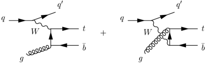
Fig. 5.: Single top quark production via the $W$-gluon fusion process.

In the rest of this section we will discuss QCD pair production of top quarks. The single top quark production modes will be discussed in Sec. 8.3.

2.1 QCD Pair Production of Top Quarks

Several reviews[cacciari97, frixione97] cover recent developments in the calculation of heavy-quark production cross sections. Here, we will summarize the main issues involved in the calculation of the $t\overline{t}$ production cross section in perturbative QCD.

The total production cross section for $p\overline{p}\rightarrow t\overline{t}$, where the proton and antiproton each have momentum $P$ ($=\sqrt{s}/2$), can be factorized in the standard way:[collins86]

$$\sigma(p\overline{p}\rightarrow t\overline{t})=\sum_{a,b}\int dx_{a}dx_{b}f_{a}^{p}(x_{a},\mu^{2})f_{b}^{\overline{p}}(x_{b},\mu^{2})\hat{\sigma}(ab\rightarrow t\overline{t};\hat{s},\mu^{2},m_{t}),$$ (15)

where the summation indices $a$ and $b$ run over light quarks and gluons. This formula expresses the total cross section in terms of the parton-parton processes $ab\rightarrow t\overline{t}$, where $a$ and $b$ are partons contained in the initial proton and antiproton carrying momentum fractions of $x_{a}$ and $x_{b}$, respectively. The parton distribution functions $f_{a}^{p}$ and $f_{b}^{\overline{p}}$ are the probability densities of finding a parton with a given momentum fraction in a proton or antiproton, and $\hat{\sigma}$ is the subprocess cross section at a parton-parton center-of-mass energy of $\hat{s}=4x_{a}x_{b}P^{2}=x_{a}x_{b}s$. The renormalization and factorization scales, here chosen to be the same value $\mu$, are arbitrary parameters. The first is introduced by the renormalization procedure, and the second by the splitting of the total cross section into perturbative ($\hat{\sigma}$) and nonperturbative ($f^{p}$, $f^{\overline{p}}$) parts. The dependence of observables on $\mu$ is an artifact of truncating the perturbation expansion at finite order; if the calculations could be carried out to all orders, the dependence on $\mu$ would vanish. For $t\overline{t}$ production, one usually takes $\mu\sim m_{t}$. Theorists typically estimate the error introduced by truncating the series by varying $\mu$ within some (arbitrary) range, such as $m_{t}/2<\mu<2m_{t}$. However, it should be recognized that neither the choice of $\mu$, nor the range over which it is allowed to vary, have physical significance.

The first calculations of the parton-parton cross section $\hat{\sigma}$ were to $O(\alpha_{s}^{2})$, that is, to leading order (LO). [georgi78] At the Tevatron, the $q\overline{q}\rightarrow t\overline{t}$ process dominates, contributing $90\%$ of the cross section, while the $gg$ process contributes the other $10\%$. (The difference between the strengths of these two subprocesses arises mainly from differences in the parton distribution functions for quarks and gluons, rather than from differences in the parton-parton cross sections.) Subsequently, several groups calculated the complete $O(\alpha_{s}^{3})$ next-to-leading order (NLO) cross section. [nason88] The NLO cross section is about $30\%$ higher than the LO cross section; the estimated uncertainty (from the sensitivity to variations in $\mu$ and changes in the parton distribution functions) is typically 10–$20\%$.

In a regime where perturbation theory is valid, the NLO contribution should be small compared to the LO terms. However, for top quark production at the Tevatron, the NLO contribution is worryingly large: for the $gg$ process it is about $70\%$ of the size of the LO terms.[laenen94] (The situation is better for the $q\overline{q}$ process, where the NLO contribution is about $20\%$ that of LO.) The large difference between the LO and NLO calculations is mainly due to processes involving the emission of soft initial state gluons. Fortunately, it is possible, through a technique called resummation, to calculate the sums of the dominant logarithms from soft gluon emission to all orders in perturbation theory. This was first carried out by Laenen, Smith, and van Neerven (LSvN).[laenen94] A difficulty arises, however, in that the resummed gluon series is divergent due to nonperturbative effects as $\alpha_{s}$ becomes large. LSvN solved this problem by introducing a new scale $\mu_{0}\gg\Lambda_{\text{QCD}}$ which is used as a cutoff to remove this divergence. They predict an increase in the cross section by $10\%$ over the NLO prediction; the uncertainty, however, is relatively large ($>10\%$), due to the dependence on $\mu_{0}$.

More recently, two other groups have performed this calculation using methods which avoid the need for an arbitrary cutoff. Berger and Contopanagos (BC),[berger95, berger96, berger98] use the technique of principal value resummation.[contopanagos93] They also find an increase of about $10\%$ over the NLO prediction, with an estimated uncertainty of about $5\%$. Bonciani, Catani, Mangano, Nason, and Trentadue (BCMNT)[catani96, bonciani98] use a slightly different scheme to avoid the divergence and treat the subleading log terms differently. They find a much smaller enhancement of the NLO cross section, on the order of $1\%$, with estimated uncertainties also of about $5\%$. A full discussion of the differences between these calculations is beyond the scope of this review, but the subject has been discussed in detail in the literature.[frixione97, berger98, bonciani98] Note, however, that if one is comparing these calculations to the present experimental results, the discrepancy between them is of no practical importance, as the difference between them is substantially smaller than the uncertainties on the experimental measurements ($\approx 30\%$). The results of various calculations for $m_{t}=175~{}\text{GeV}/c^{2}$ are compared in Table 2. A plot of the various cross sections is given in Fig. 6.

Table 2.: Results of several different $p\overline{p}\rightarrow t\overline{t}$ calculations, for $m_{t}=175~{}\text{GeV}/c^{2}$ and $\sqrt{s}=1.8~{}\text{TeV}$. Note that the LSvN result uses an older set of structure functions, which makes it systematically low compared to the other results.[berger96]

Calculation	Type	Structure Function	$\sigma_{t\overline{t}}$
(1) Exact NLO[nason88, bonciani98]	NLO only	MRSR2[martin96]	$4.87^{+0.30}_{-0.56}~{}\text{pb}$
(2) LSvN[laenen94]	Resummed	MRSD′[martin93]	$4.94^{+0.71}_{-0.45}~{}\text{pb}$
(3) BC[berger98]	Resummed	CTEQ3[cteq95]	$5.52^{+0.07}_{-0.42}~{}\text{pb}$
(4) BCMNT[bonciani98]	Resummed	MRSR2[martin96]	$5.06^{+0.13}_{-0.36}~{}\text{pb}$

Fig. 6.: Results of top quark production cross section calculations for $\sqrt{s}=1800~{}\text{GeV}$. The upper group of curves are for $t\overline{t}$ production,[nason88, laenen94, berger98, bonciani98] and the lower curve is for single top quark production.[heinson97b] Note that the LSvN result uses an older set of structure functions, and is thus systematically low compared to the other results.[berger96]

It should be appreciated that these cross sections are extremely small — about ten orders of magnitude smaller than the total inelastic $p\overline{p}$ cross section. Of the five trillion or so collisions which have occurred at each of the CDF and DØ interaction regions during Run 1, one expects about 600 $t\overline{t}$ pairs to have been produced. It should also be noted that all these calculations assume a minimal form of the Standard Model. Certain extensions to the SM, such as models with two Higgs doublets or supersymmetry, predict $t\overline{t}$ production cross sections which are different from that of the SM by a few percent. [hollik97]

2.2 Top Quark Hadronization and Decay

Within the Standard Model, the dominant decay of a top quark is via $t\rightarrow Wb$, with a branching ratio of nearly $100\%$. The decays $t\rightarrow Ws$ and $t\rightarrow Wd$ are also allowed, but are suppressed by factors of $10^{-3}$–$10^{-4}$ by the Cabibbo-Kobayashi-Maskawa (CKM) mixings.[pdg96] Other decays, such as flavor-changing neutral current (FCNC) decays, are predicted to be many orders of magnitude smaller. We will discuss these further in Sec. 7.

Owing to the large mass of the top quark, its lifetime is extremely short ($\Gamma\approx 1.5~{}\text{GeV}$, corresponding to $\tau\approx 5\times 10^{-25}~{}\text{s}$); so short, in fact, that at Tevatron energies it decays before it has a chance to hadronize.[orr91] This implies that a decaying top quark can be treated as a free particle. Note, however, that it isn’t just the large mass of the top quark which gives it its short lifetime, but also the fact that it has a CKM-allowed decay into a $b$-quark. A fourth-generation down-type quark $b^{\prime}$ of mass comparable to the top quark might still have a long lifetime if all its decay modes were suppressed by the CKM mixings.

A $t\overline{t}$ final state contains two $t\rightarrow Wb$ decays. The two $b$-quarks will form jets, while each $W$ boson will decay into either a lepton-neutrino or a quark-antiquark pair. To a good approximation, each possible decay of the $W$ boson is equally probable; however, one must remember to count each quark flavor three times, since quarks come in three colors. Therefore, the probability for a $W$ boson to decay into each of the three lepton flavors is about $1/9$, while the probability for it to decay into the two available quark final states is about $2/3$.

Table 3.: Decay modes for a $t\overline{t}$ pair and branching fractions.

		$W\rightarrow e\nu_{e}$	$W\rightarrow\mu\nu_{\mu}$	$W\rightarrow\tau\nu_{\tau}$	$W\rightarrow q\overline{q}$
		(1/9)	(1/9)	(1/9)	(2/3)
$W\rightarrow q\overline{q}$	(2/3)	$12/81$	$12/81$	$12/81$	$36/81$
		($e+\text{jets}$)	($\mu+\text{jets}$)	($\tau+\text{jets}$)	(all jets)
$W\rightarrow\tau\nu_{\tau}$	(1/9)	$2/81$	$2/81$	$1/81$
		($e\tau$)	($\mu\tau$)	($\tau\tau$)
$W\rightarrow\mu\nu_{\mu}$	(1/9)	$2/81$	$1/81$
		($e\mu$)	($\mu\mu$)
$W\rightarrow e\nu_{e}$	(1/9)	$1/81$
		($ee$)

Since there are two top quarks in each event, and since the $W$ bosons decay independently of each other, the events can be classified according to how the $W$ bosons decay (see Table 3).

• Events in which both $W$ bosons decay leptonically are called dilepton events. Since tau leptons are difficult to identify, the particular dilepton channels which have been most studied are the $ee$, $\mu\mu$, and $e\mu$ channels. These final states have the signature of two high-$p_{T}$ leptons, a large imbalance in the total transverse momentum (“missing-$E_{T}$,” or ${\hbox{$E$\kern-6.00006pt\lower-0.43057pt\hbox{/}}}_{T}$), and two $b$-jets. These events are expected to have small backgrounds (especially the $e\mu$ channel). However, as can be seen from Table 3, they also have small branching fractions, with all three of these channels comprising only about $4/81\approx 4.9\%$ of $t\overline{t}$ decays. (There is also a small contribution from the $\tau$ lepton channels. For example, $t\overline{t}\rightarrow b\overline{b}\,e\nu\,\tau\nu\rightarrow b\overline{b}\,e\nu\,e\nu\nu$ can contribute to the $ee$ channel.) Dilepton events also have the drawback of containing two unobserved neutrinos in the final state, which prevents complete reconstruction of the event kinematics.

  Several recent analyses have also considered the $e\tau$ and $\mu\tau$ channels. These will be discussed in Sec. 5.2.

• Events in which one $W$ boson decays leptonically and the other decays into quarks are called lepton+jets events. Those which have been studied are the $e+\text{jets}$ and $\mu+\text{jets}$ channels. They are characterized by a final state containing one high-$p_{T}$ lepton, large ${\hbox{$E$\kern-6.00006pt\lower-0.43057pt\hbox{/}}}_{T}$, and four jets, two of which are $b$-jets. Compared to the dilepton channels, the lepton+jets channels have a much larger cross section — the branching ratio for each is about $4/27\approx 15\%$. (Again, there is a small additional contribution from $\tau$ lepton channels.) The final state contains only one neutrino, so there is sufficient information to completely reconstruct the event (once a particular set of assignments of jets to the final state partons is assumed). The disadvantage of these channels, however, is a large background from inclusive $W$ boson production with associated jets, plus a smaller background from QCD jet production.

• Events in which both $W$ bosons decay into quarks are called all-jets events. This final state consists of six jets, of which two are $b$-jets, no high-$p_{T}$ leptons, and small ${\hbox{$E$\kern-6.00006pt\lower-0.43057pt\hbox{/}}}_{T}$. This channel boasts the largest branching ratio ($\approx 44\%$ of the total). Unfortunately, that is more than countered by a huge background from QCD multijet processes. Nevertheless, it is still possible to isolate a $t\overline{t}$ signal in this channel. The techniques for doing so will be discussed in Sec. 5.

2.3 Modeling Top Quark Events

Accurate modeling of the kinematics of $t\overline{t}$ production and decay is essential for extracting reliable information from the data. The most widely used general-purpose model is that provided by the herwig Monte Carlo program.[herwig] herwig models $t\overline{t}$ production starting with the leading-order hard process, choosing the parton momenta according to the weight given by the matrix element of the process. Gluon emission from both the initial and final states is modeled using leading-log QCD evolution,[altarelli77] keeping track of the correlations induced by color strings between partons. Each top quark is then decayed to a $W$ boson and a $b$-quark, and partons remaining in the final state are hadronized into jets. Products of interactions among the beam remnants, called the underlying event, are also included in the model. Detector effects are then added using a model of the detector response to the physical objects.

There have been several studies comparing the predictions of parton shower Monte Carlo programs such as herwig to the more explicit calculations. Frixione et al.[frixione95] compare herwig to the full NLO calculation. They distinguish two types of quantities: those which are delta functions at leading order, such as $p_{T}(t\overline{t})$ and $\Delta\phi(t\overline{t})$, and those which are nontrivial at leading order, such as $p_{T}(t)$, $\eta(t)$, and $m_{t\overline{t}}$. For the latter, nontrivial, set of quantities they find good agreement between the Monte Carlo predictions and the full NLO calculation. For the other quantities, however, they find significant disagreement in the low-$p_{T}$ region (see Fig. 7). They interpret this as a deficiency in the NLO calculation due to the lack of resummation effects, and conclude that herwig is more reliable than the NLO calculation in that region. Orr et al.[orr97] compare an $O(\alpha_{s}^{3})$ calculation of gluon emission in $t\overline{t}$ events to herwig; they find that herwig seems to generate too much final state radiation. On the other hand, Mrenna et al. [mrenna97] compare a resummed calculation for $t\overline{t}$ production to a different Monte Carlo program, pythia,[pythia] and find that the latter generates too little radiation. These discrepancies are probably not large enough to be important for the current experimental results. But they will have to be understood better for the next round of experiments — radiation effects are already one of the dominant uncertainties for the present measurements of the mass of the top quark, so the precision of the measurement may not improve much until these effects are better understood.

Fig. 7.: Transverse momentum of the $t\overline{t}$ pair: NLO calculation compared to herwig. The inset magnifies the low $p_{T}$ portion of the plot on a linear scale. The herwig prediction has been scaled by a constant factor of $K=1.34$. From Ref.[frixione97].

3 Detecting the Top Quark

In this section, we discuss some of the experimental aspects of detecting the top quark. We first summarize the apparatus used: the Tevatron collider and the CDF and DØ detectors. We then discuss the procedures used by the experiments to identify final state objects, such as electrons, muons, and jets. We conclude this section with a summary of the distinctive characteristics of the top quark signal and its principal backgrounds.

3.1 The Accelerator

The Fermilab $p\overline{p}$ collider[tevrev] in Batavia, Illinois is the world’s highest energy particle accelerator, with a center-of-mass energy of $1800~{}\text{GeV}$. It is the only facility at present capable of producing top quarks for direct study.

A schematic of the accelerator complex is shown in Fig. 8. Negative hydrogen ions are first accelerated to $750~{}\text{keV}$ by an electrostatic Cockroft-Walton accelerator and then further boosted to $400~{}\text{MeV}$ by a $150~{}\text{m}$ long linear accelerator. At the end of this accelerator, the electrons are stripped from the ions and the resulting protons enter the booster. This $75~{}\text{m}$ radius synchrotron accelerates the protons to $8~{}\text{GeV}$. From there they are injected into the Main Ring.

Fig. 8.: Schematic of the Fermilab accelerator complex (not to scale). From Ref.[joeythesis].

The Main Ring is a large ($1000~{}\text{m}$ radius) synchrotron, composed of conventional electromagnets, which accelerates protons and antiprotons up to $150~{}\text{GeV}$ for injection into the Tevatron. It also serves as a source of $120~{}\text{GeV}$ protons for producing antiprotons.[apsource] The antiprotons are collected from the production target using a lithium lens, momentum-selected around $8~{}\text{GeV}$, and then directed first into the Debuncher and then into the Accumulator. These are two concentric storage rings with radii of about $80~{}\text{m}$. There, the antiprotons are stochastically cooled[stcool] to reduce their momentum spread. When enough antiprotons have been accumulated (stacked), they are extracted into the Main Ring, accelerated, and injected into the Tevatron.

The Tevatron, a synchrotron made from superconducting magnets, is situated just below the Main Ring. In collider mode, the Tevatron is filled with six bunches of protons and six bunches of antiprotons, circulating in opposite directions. The beams are accelerated to the maximum energy of $900~{}\text{GeV}$ each and brought into collision at the CDF and DØ experimental areas. The beams are typically kept colliding for about 20 hours, after which the machine is emptied and refilled with new batches of protons and antiprotons. The length of each bunch is about $50~{}\text{cm}$, dictated by the accelerator RF system, giving a luminous region at each interaction point which is roughly Gaussian with a longitudinal width of about $30~{}\text{cm}$. This relatively long bunch length produces a degradation of the transverse energies at the trigger level because the information about the position of the interaction point is not available at the early stages of triggering. At CDF, it also results in a substantial loss of acceptance of the vertex detector for $b$-quarks (see Sec. 3.3.6.2).

The Main Ring lies mostly in a plane, except at the CDF and DØ experimental areas where it is bent into overpasses to allow room for the detectors. The separation between the Main Ring and the Tevatron is $5.8~{}\text{m}$ at CDF and $2.3~{}\text{m}$ at DØ. At CDF, the overpass clears the detector. At DØ, however, the Main Ring overpass goes through the outer (coarse hadronic) part of the calorimeter. This is unfortunate because during normal collider data-taking, the Main Ring is used for antiproton production and losses from the Main Ring may deposit energy in the detectors, thereby increasing background. DØ rejects much of this background at the trigger level by rejecting triggers that occur during injection into the Main Ring, when losses are large. Some triggers are also disabled whenever a Main Ring bunch passes through the detector or when losses are registered in scintillation counters around the Main Ring. This results in a loss of about $15\%$ of the available livetime. The problem of Main Ring contamination is far less severe at CDF; even so, CDF observes occasional events with extra energy from the Main Ring. These events are rejected offline.

The collider was commissioned with a short run in 1985, followed by the first high luminosity run in 1988–1989. Only the CDF detector took data during that run, which had a peak luminosity of about $2\times 10^{30}~{}\text{cm}^{-2}\,\text{s}^{-1}$ (a factor of two greater than the design luminosity). The second series of runs took place over the period 1992–1996, during which a peak luminosity of $2\times 10^{31}~{}\text{cm}^{-2}\,\text{s}^{-1}$ was achieved. This period was divided into three runs, designated Run 1a, Run 1b, and Run 1c; the delivered integrated luminosities for these runs were about $23~{}\text{pb}^{-1}$, $122~{}\text{pb}^{-1}$, and $17~{}\text{pb}^{-1}$, respectively. The results covered in this review are from this running period. Table 4 reviews the major parameters of the collider.

Table 4.: Parameters of the Fermilab Tevatron collider for Run 1.

Accelerator radius	$1000~{}\text{m}$
Maximum beam energy	$900~{}\text{GeV}$
Injection energy	$150~{}\text{GeV}$
Peak luminosity	$\approx 2\times 10^{31}~{}\text{cm}^{-2}\,\text{s}^{-1}$
Number of bunches	6 $p$, 6 $\overline{p}$
Intensity per bunch	$\approx 10^{11}p$, $\approx 5\times 10^{10}\overline{p}$
Crossing angle	$0^{\circ}$
Bunch length	$50~{}\text{cm}$
Transverse beam radius	$\approx 25~{}\text{$\mu$m}$
Fractional energy spread	$0.15\times 10^{-3}$
RF frequency	$53~{}\text{MHz}$
$\overline{p}$ stacking rate	$\approx 3.5\times 10^{10}/\text{hour}$
Beam crossing frequency	$290~{}\text{kHz}$
Period between crossings	$3.5~{}\text{$\mu$s}$

3.2 The CDF and DØ Detectors

The two collider experiments at the Fermilab Tevatron, CDF [cdfdetector, cdfsvx2] and DØ,[d0detector] are illustrated in Figs. 9 and 10. Both were designed to study high-$p_{T}$ interactions and feature large angular coverage and good identification and measurement of electrons, muons, and jets. The layouts of both detectors are broadly similar. Moving outwards from the interaction point, one first encounters tracking detectors, which measure the trajectories of charged particles, then calorimeters, which measure the energies of jets and of electromagnetic showers, and finally an outer set of tracking chambers, which identify and measure muons that penetrate the calorimeter. There are tradeoffs between these various systems: of the two detectors, CDF puts relatively more emphasis on tracking, while DØ emphasizes calorimetric measurements.

We use a coordinate system centered on the detector, with the $z$-axis along the beam direction, and the $x$- and $y$-axes defining the transverse plane. We also use the polar angle $\theta$, the azimuthal angle $\phi$, and the pseudorapidity $\eta$, defined as $\eta\equiv-\ln(\tan{\theta/2})$. It is also common to calculate the angle between directions of two objects in terms of the distance between them in the $(\eta,\phi)$ plane, as $R=\sqrt{(\Delta\eta)^{2}+(\Delta\phi)^{2}}$.

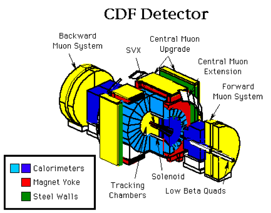
Fig. 9.: The CDF detector, in isometric view (left) and cross sectional view of one quadrant (right). The detector is forward-backward symmetric about the interaction region, which is at the lower-right corner of the cross sectional view. SVX, VTX, CTC, and CDT are tracking detectors, CEM, CHA, WHA, PEM, PHA, FEM, and FHA are calorimeters, CMU, CMP, CMX, and FMU are muon chambers, BBC is a scintillation counter, and CPR and CES are multiwire proportional chambers. From Ref.[cdftopprd94].

Fig. 10.: The DØ detector, in both isometric and cross sectional views. CF, EF, and SAMUS are the three regions of the muon system (the small angle SAMUS system is not used in top analyses). From Ref.[d0detector].

3.2.1 CDF

At the core of the CDF detector is a cylindrical tracking volume contained within a large ($4.8~{}\text{m}$ long by $1.5~{}\text{m}$ radius) superconducting solenoid that generates a field of $1.4~{}\text{T}$. Immediately surrounding the beam pipe is the four-layer silicon vertex detector (SVX). This $51~{}\text{cm}$ long device provides precise track reconstruction in the plane normal to the beam, measuring track impact parameters with a resolution of $\sigma=(13+40\ (\text{GeV}/c)/p_{T})~{}\text{$\mu$m}$. This is sufficiently precise to identify displaced vertices from $b$- and $c$-quark decays. The luminous region at CDF has a $1\sigma$ width of about $30~{}\text{cm}$, giving the SVX a geometrical acceptance of about $67\%$. The original SVX detector suffered significant radiation damage during Run 1a, but was replaced before the start of Run 1b with a similar detector equipped with radiation-hard electronics.[cdfsvx2] Outside the SVX is a vertex drift chamber (VTX), which is used to measure the $z$ position of the interaction vertex to a precision of $1~{}\text{mm}$. The VTX in turn is mounted inside of the central tracking chamber (CTC), a large cylindrical drift chamber which measures the curvature of tracks passing through the magnetic field.

Surrounding the tracking volume are the calorimeters. There are three distinct calorimeter regions: central ($|\eta|<1.1$), end-plug, and forward. In each region, there is an electromagnetic calorimeter backed by a hadronic calorimeter. The electromagnetic calorimeters use lead as an absorber, while the hadronic calorimeters use iron. The active media are scintillator tiles in the central region and gas proportional chambers in the end-plug and forward regions. The tower geometry is projective — that is, the towers point to the nominal interaction point — with a cell size in the central region of $\Delta\eta\times\Delta\phi\approx 0.1\times 0.25$. A layer of proportional wire chambers is located at shower maximum in the central electromagnetic calorimeter, and additional proportional chambers located between the solenoid and the CEM sample the early development of electromagnetic showers in the solenoid. The energy resolution, $\sigma(E)/E$, of the calorimeters in the central region is about $13.7\%/\sqrt{E}\oplus 2\%$ for electromagnetic showers and about $50\%/\sqrt{E}\oplus 3\%$ for single hadrons. The thickness of the central calorimeters is about 18 radiation lengths for the electromagnetic section and 4.5 interaction lengths for the hadronic section.

Muons are identified using drift chambers surrounding the calorimeter, the central muon system and central muon upgrade. There is about $0.6~{}\text{m}$ of steel between these two sets of chambers. Together, they provide coverage out to about $|\eta|<0.6$. Coverage is extended out to about $|\eta|<1.1$ by the chambers of the central muon extension.

3.2.2 DØ

DØ is the newer of the two detectors, commissioned during the summer of 1992. Its tracking volume is relatively compact ($1.35~{}\text{m}$ long by $0.78~{}\text{m}$ radius) and nonmagnetic. Nested around the beam pipe are the vertex drift chamber (VTX), a transition radiation detector (TRD), and the central drift chamber (CDC). The tracking volume is capped on the ends by two forward drift chambers (FDCs). The trajectories of tracks of charged particles can be measured with a resolution of $2.5~{}\text{mrad}$ in $\phi$ and $28~{}\text{mrad}$ in $\theta$, and the $z$-coordinate of the interaction vertex can be measured with a resolution of about $8~{}\text{mm}$. The central tracking system also measures the ionization of tracks in order to distinguish between single charged particles and $e^{+}e^{-}$ pairs from photon conversions.

The calorimeter is divided into three parts: the central calorimeter (CC) and the two end calorimeters (ECs). They each consist of an inner electromagnetic (EM) section, a fine hadronic (FH) section, and a coarse hadronic (CH) section. The absorber in the EM and FH sections is depleted uranium; in the CH section, it is a mixture of stainless steel and copper. The active medium in all cases is liquid argon.

The EM sections of the calorimeters are about 21 radiation lengths deep, and are read out in four longitudinal segments (layers). The hadronic sections are 7–9 interaction lengths deep, with either four (CC) or five (EC) layers. The transverse segmentation is pseudoprojective (that is, although each cell is nonprojective, they form towers which are), with a cell size of $\Delta\eta\times\Delta\phi=0.1\times 0.1$. In the third layer of the EM calorimeter, near the shower maximum, the segmentation is twice as fine in each direction, with a cell size of $\Delta\eta\times\Delta\phi=0.05\times 0.05$. The energy resolution is about $15\%/\sqrt{E}\oplus 0.4\%$ for electromagnetic showers and $50\%/\sqrt{E}$ for single hadrons. The resolution is substantially worse, however, in the transition regions between the CC and the ECs, due to the presence of a large amount of uninstrumented material. Some of the energy that would otherwise be lost is collected in extra argon gaps mounted on the ends of the calorimeter modules (“massless gaps”) and in scintillator tiles mounted between the CC and EC cryostats (intercryostat detectors, or ICDs).

The DØ muon system consists of a “wide angle” system, covering $|\eta|<1.7$, and a “small angle” (forward) system, extending the coverage out to $|\eta|<3.3$. For studying top quark decays, DØ uses only the wide angle system. This system consists of four planes of proportional drift tubes in front of magnetized iron toroids, with a magnetic field of $1.9\ \text{T}$, and two groups of three planes of proportional drift tubes behind the toroids. The magnetic field lines and the wires in the drift tubes are oriented transversely to the beam direction. The muon momentum is measured from the muon’s deflection angle in the magnetic field of the toroid. The total amount of material in the calorimeter and iron toroids varies between 13 and 19 interaction lengths, making the background from hadronic punchthrough negligible. In addition, the compact central tracking volume reduces backgrounds to prompt muons from in-flight decays of $\pi$ and $K$ mesons. During Run 1b, the forward muon chambers suffered radiation damage that reduced their efficiency. Midway through the run, however, the damage was repaired. As a result, the DØ top quark analyses do not use forward muons for the first half of Run 1b.

3.3 Particle Identification

This section summarizes the algorithms used by the two experiments to identify the various final-state objects in candidate $t\overline{t}$ events. For more details, see Refs.[cdftopprd94, d0topprd], and [d0ljtopmassprd].

3.3.1 Quarks and Gluons

As a quark or gluon leaves the site of a hard scattering it cannot remain free, but instead hadronizes (or fragments) into a collection or jet of (colorless) hadronic particles. This collection tends to lie in a cone around the direction of motion of the original parton, and will show up in a calorimeter as an extended cluster of energy. In order to compare measurements with theoretical predictions it is necessary to have a precise definition of a jet: that is, one must specify how calorimetric energy depositions (cells) are to be clustered into jets. This algorithm is, in principle, arbitrary. However, at hadron colliders, it is conventional to define jets by taking all calorimeter cells which lie within a cone of fixed radius $R$ in the $(\eta,\phi)$ plane. This choice is convenient because jets are approximately circular in these variables; further, the $R$-width of jets of a given $E_{T}$ is independent of the jet rapidity. More importantly, this definition can be readily implemented in phenomenological calculations, thereby facilitating the comparison of theory with experimental data.[snowmass]

In principle, not only is the jet algorithm arbitrary but also the cone radius $R$. In practice, the choice of cone radius involves several competing considerations. Jets are extended objects, composed of a collection of particles from hadronization of the progenitor parton. The jet will be further broadened as the particles undergo showering in a calorimeter. Consequently, if $R$ is too small, a substantial portion of the energy from the progenitor parton will lie outside of the jet cone. This effect can be corrected for on average. However, the smaller the cone radius, the larger the energy correction that must be applied and, therefore, the worse the energy resolution of the corrected jet. On the other hand, if $R$ is made too large, one cannot resolve the energy depositions arising from closely spaced partons; instead, the depositions get merged together into a single jet. This is of particular concern for $t\overline{t}$ events, which tend to have many jets in the final state. The optimum choice for $R$ for $t\overline{t}$ physics depends somewhat on the structure of the calorimeter, but appears to be around $0.4$–$0.5$: CDF chooses $R=0.4$, and DØ uses $R=0.5$.

Although both experiments have a resolution for single hadrons that scales as $\sigma(E)/E\sim 50\%/\sqrt{E}$, the resolution achievable for jets is typically $\sigma(E)/E\sim 100\%/\sqrt{E}$. Most of the particles comprising a jet are of relatively low energy, in which region nonlinear effects in calorimeter response become important. Jet resolutions are also degraded by effects such as gluon radiation, differences in calorimeter response to hadrons and electrons, energy falling out of the jet cone, and contamination from hadrons from the underlying event.

The measurement of jet energies is subject to numerous systematic effects, for which one must correct. These include:

• The intrinsic response of the calorimeter to jets.

• Calorimeter nonuniformities, and regions with uninstrumented material (such as cracks between modules).

• Energy from the underlying event and, at DØ, noise from the radioactive decay of the uranium absorber.

• QCD radiation of gluons outside of the jet cone.

• The spreading of particle showers outside of the jet cone in the calorimeter.

The procedures involved in performing these corrections are quite complicated;[cdftopprd94, cdf4jet93] we shall therefore only summarize the strategies used.

• Dijet events, in which the transverse energies of the two jets should balance, can be used to calibrate one region of the detector relative to another, better characterized, region.

• Events with an electromagnetic cluster recoiling against a jet can be used to calibrate hadronic calorimeters relative to electromagnetic calorimeters.

• The absolute scale of electromagnetic calorimeters can be determined by comparing electron energies to their momenta measured in the tracking system (at CDF) or by using the known masses of resonances such as the $Z$, the $\pi^{0}$, and the $J/\psi$ (at DØ).[d0wmassprd1b]

• Contributions from the underlying event and noise can be studied using Monte Carlo simulations, and by comparing data taken under differing trigger conditions and luminosities.

• The broadening of showers in calorimeters can be studied using test beams.[tb90l1a] Monte Carlo simulations are used to model the distribution of particles produced during hadronization of partons.

CDF and DØ apply jet corrections at different points in their analyses. This should be kept in mind when comparing selections involving jet energies. CDF does not use the jet corrections for measuring cross sections (except in the all-jets channel), but does apply them for the mass measurement, after the event sample has been selected. DØ, on the other hand, applies most corrections before making any analysis selections. The corrections include effects of jets spreading in the calorimeter, but not of particles originating from gluons radiated outside of the jet cone. DØ applies an additional correction in its mass analysis to include this effect.

It is important to realize that there is not necessarily any one-to-one correspondence between quarks and gluons in the final state of the hard scattering and the detected jets. A jet may have insufficient energy to be selected as a jet (a typical requirement is that the jet energy be at least $15~{}\text{GeV}$), or two partons may be sufficiently close together that their energies are merged together during jet reconstruction. Conversely, if a parton radiates a gluon with a large relative transverse momentum, then that gluon may be reconstructed as a separate jet. Moreover, nonclassical effects, such as partonic interference, are always present and place a fundamental limit on the validity of identifying a given jet with a specific progenitor parton.

3.3.2 Electrons

Electron identification is based on finding isolated clusters of energy in the electromagnetic sections of the calorimeter, along with a matching track in the central detector from a charged particle. Additional requirements are then made to further suppress background from QCD jets. The exact requirements vary between experiments and among different analyses. However, typical requirements are:

• The fraction $f_{E}$ of the cluster energy in the electromagnetic sections of the calorimeter should be $\gtrsim 90\%$.

• The shape of the cluster should be consistent with expectations from test beams or Monte Carlo simulations.

• The track momentum $p$ should be consistent with the cluster energy $E$, $E/p\sim 1$ (CDF only).

• The distance between the cluster and the extrapolated track should be small.

• A track ionization consistent with a singly charged particle (DØ only). Photon conversions into $e^{+}e^{-}$ pairs typically deposit twice the charge expected from one minimum ionizing particle.

• Transition radiation information consistent with an electron (used in DØ dilepton analyses).

• Isolation, based either on calorimetry or (at CDF only) on tracking. One typically requires that the energy or momentum in the region around the electron candidate be small.

CDF accepts electrons in the central calorimeter with $|\eta|<1.0$. For the dilepton channels, one electron may also be in the plug calorimeter, thereby providing extra coverage in the range $1.20<|\eta|<1.35$. DØ accepts electrons out to $|\eta|<2.5$ for the dilepton channels and out to $|\eta|<2.0$ for the lepton+jets channels (although the efficiency is poor in the transition region between the central and end cryostats, $1.1<|\eta|<1.5$).

3.3.3 Muons

At CDF, muons are identified by requiring a match between a CTC track and a track segment in the muon chambers. This provides coverage out to $|\eta|<1.0$. For dilepton channels, CDF also identifies muons in sections of the detector where there is no coverage from muon chambers but good central tracking. This extends coverage out to $|\eta|<1.2$, and fills in coverage of azimuthal holes for $|\eta|<1.0$. Additional selections are made on the following variables:

• The energy deposited in the calorimeters along the muon track.

• The distance of closest approach of the muon track to the beam line.

• The distance in $z$ between the interaction vertex and the muon track.

• The distance between the extrapolated CTC track and the track segment in the muon chambers.

• Isolation, defined in a similar manner as for electrons except that calorimeter-based isolation is used when there is no matching track in the muon chambers.

DØ identifies muons by tracks in the muon chambers. A matching central detector track is not required, but if one is present, it is taken into account in the momentum measurement. The following additional criteria are used for DØ’s muon selection:

• The line integral over the magnetic field $>2.0~{}\text{$\text{T}\cdot\text{m}$}$. This rejects muons which pass through the thin portion of the toroid around $|\eta|\approx 0.9$. Such muons bend less so their momenta are poorly measured. They also have a larger contamination from hadronic punchthrough.

• The energy deposited along a muon track in the calorimeter must be at least that expected for a muon ($\sim 2$–$3~{}\text{GeV}$).

• The impact parameter between the muon track and the interaction vertex must be small.

• Muons are defined as either isolated or nonisolated, depending on whether the distance in the $\eta-\phi$ plane between the muon and the closest jet is greater than or less than $0.5$, respectively.

For the first portion of Run 1b, when the forward muon chambers were affected by radiation damage, the muon selection was restricted to the central region, with $|\eta|<1.0$. For other run periods, muon acceptance extended out to $|\eta|<1.7$.

3.3.4 $\tau$ Leptons

Tau leptons are difficult to identify. A $\tau$ will decay into an electron or a muon about $36\%$ of the time, and the only observable difference between the decays $W\rightarrow\ell\nu$ and $W\rightarrow\tau\nu\rightarrow\ell\nu\nu\nu$ is that the lepton spectrum is somewhat softer in the latter case. If the $\tau$ decays hadronically, it can be detected as a narrow jet with either one or three associated tracks. The branching ratios for these “one-prong” and “three-prong” hadronic decays are about $50\%$ and $14\%$, respectively.[pdg96] The challenge is to reject the large background from quark and gluon jets. CDF manages this with two complementary techniques, one “track-based” and the other “calorimeter-based.”[cdftoptotau97]

The track-based technique is sensitive only to one-prong $\tau$ decays. It starts by finding an isolated, high-$p_{T}$ ($>15~{}\text{GeV}/c$), central ($|\eta|<1.0$) track. The isolation requirement is based on the sum of the $p_{T}$ values of all tracks in a $\Delta R$ cone around the high-$p_{T}$ track. This discriminates between $\tau$ leptons and jets. The energy in the calorimeter around the track is required to be consistent with the track momentum. In addition, candidates consistent with being electrons (large fractional energy in the electromagnetic calorimeter) or muons (energy deposition consistent with a minimum ionizing particle) are rejected.

The calorimeter-based technique starts from a calorimeter cluster with $|\eta|<1.2$ with either one or three isolated charged tracks pointing at it. (The tracks must have $p_{T}>1~{}\text{GeV}/c$ and lie within a $10^{\circ}$ cone around the centroid of the cluster.) About $73\%$ of one-prong and $41\%$ of three-prong decays are expected to contain $\pi^{0}$s, which can be identified from their $\pi^{0}\rightarrow\gamma\gamma$ decays. The candidate is rejected if there are more than two $\pi^{0}$s. The $\tau$ lepton $p_{T}$ is defined as the sum of the transverse momenta of all candidate tracks plus the transverse momenta of all $\pi^{0}$s; it must satisfy $p_{T}>15~{}\text{GeV}/c$. Also, the total invariant mass constructed from the tracks and the $\pi^{0}$s must be $<1.8~{}\text{GeV}/c^{2}$. The calorimeter cluster must be narrow, and its energy must be consistent with the total $\tau$ momentum. Finally, clusters consistent with being electrons or muons are removed.

The efficacy of the calorimeter-based selection is demonstrated in Fig. 11, which shows the track multiplicity for a monojet sample which required one jet with $15<E_{T}<40~{}\text{GeV}$, $20<$${\hbox{$E$\kern-6.00006pt\lower-0.43057pt\hbox{/}}}_{T}$$<40~{}\text{GeV}$, and no other jet with $E_{T}>7~{}\text{GeV}$. The excess in the one and three track bins from $W\rightarrow\tau\nu$ is apparent; it is also seen that the calorimeter-based selection drastically reduces the background. About $45\%$ of hadronic $\tau$ decays satisfy the kinematic requirements; of these, about $55\%$ are identified by this algorithm.

Fig. 11.: Track multiplicity in the monojet data sample. a) No $\tau$ identification requirements. b) All calorimeter-based $\tau$ identification requirements, except for track multiplicity. From Ref.[cdftoptotau97].

3.3.5 Neutrinos

Neutrinos do not interact in the detector with any significant probability, and therefore cannot be observed directly. Instead, their presence is inferred from an imbalance in the total transverse momentum in the event. Because the remnants of the spectator partons escape down the beam pipe, the longitudinal component of the neutrino momentum cannot be measured.

The missing transverse energy $\vec{\mbox{${\hbox{$E$\kern-6.00006pt\lower-0.43057pt\hbox{/}}}_{T}$}}$ is defined by

$$\mbox{${\hbox{$E$\kern-6.00006pt\lower-0.43057pt\hbox{/}}}_{T}$}_{x} =-\sum_{i}E_{i}\sin\theta_{i}\cos\phi_{i},$$ (16)

$$\mbox{${\hbox{$E$\kern-6.00006pt\lower-0.43057pt\hbox{/}}}_{T}$}_{y} =-\sum_{i}E_{i}\sin\theta_{i}\sin\phi_{i},$$ (17)

where the sums are over all calorimeter cells. If there are muons in the final state, then their transverse momenta should also be subtracted from $\vec{\mbox{${\hbox{$E$\kern-6.00006pt\lower-0.43057pt\hbox{/}}}_{T}$}}$. (Some analyses make use of the ${\hbox{$E$\kern-6.00006pt\lower-0.43057pt\hbox{/}}}_{T}$ measured by the calorimeter without correcting for muons. This quantity will be denoted by ${\hbox{$E$\kern-6.00006pt\lower-0.43057pt\hbox{/}}}_{T}^{\text{cal}}$.) The resolution of ${\hbox{$E$\kern-6.00006pt\lower-0.43057pt\hbox{/}}}_{T}$ is usually parameterized in terms of the total transverse energy in the event (a scalar sum). CDF quotes[cdftopprd94] a resolution of $\sigma(\mbox{${\hbox{$E$\kern-6.00006pt\lower-0.43057pt\hbox{/}}}_{T}$})=0.7\sqrt{\sum{E_{T}}}$ (units in GeV), while DØ quotes[d0topprd] $\sigma(\mbox{${\hbox{$E$\kern-6.00006pt\lower-0.43057pt\hbox{/}}}_{T}$})=1.08~{}\text{GeV}+0.019\sum E_{T}$.

3.3.6 Tagging $b$-Jets

A prominent feature of $t\overline{t}$ decays is that each event contains two $b$-quarks. This is in contrast to the principal backgrounds, in which heavy flavors are expected to be relatively rare. Clearly, a method for identifying, or tagging, $b$-jets would be valuable in separating $t\overline{t}$ events from background. The two strategies developed for doing this, soft-lepton tagging (SLT) and displaced-vertex tagging (SVX, using the silicon vertex detector), are discussed below.

3.3.6.1 $b$-Tagging with Soft Leptons

Approximately $22\%$ of the time, a decaying $b$-quark will yield a muon, either directly or through a sequential decay via a $c$-quark. The branching ratio to electrons is also $22\%$. One method of $b$-tagging is based on observing such leptons close to a jet. These leptons are much softer than the leptons from $W$ boson decay, typically below about $20~{}\text{GeV}/c$. (See Fig. 12.) Because they are soft and not isolated, their detection efficiencies are significantly lower than for the high-$p_{T}$ isolated leptons from $W$ boson decay.

Fig. 12.: $p_{T}$ spectra of leptons from decays of $b$- and $c$-quarks in $t\overline{t}$ Monte Carlo events ($m_{t}=160~{}\text{GeV}/c^{2}$). From Ref.[cdftopprd94].

Both experiments tag $b$-jets with this method. CDF uses both electron and muon tags, while, in the analyses reviewed here, DØ uses only muon tags. Without a central magnetic field, electron tagging is less effective at DØ. However, even at CDF, the electron tags play a relatively minor role: the efficiency for electron tagging is about $1/3$ of that for muon tagging. Another difference is that CDF selects soft leptons with $p_{T}>2~{}\text{GeV}/c$, while DØ requires $p_{T}>4~{}\text{GeV}/c$ because muons with lower momenta have insufficient energy to traverse the calorimeter and toroid. However, DØ has a larger muon acceptance than CDF. In addition, the fake rate for muon tags is significantly smaller at DØ, due both to the large amount of material in the calorimeter and muon toroid (which reduces hadronic punchthrough) and the small size of the tracking volume (which reduces background due to in-flight $\pi/K$ decays). When all factors are accounted for, the probability of finding a lepton tag in a $t\overline{t}$ decay is nearly the same for both experiments, about $20\%$.

3.3.6.2 $b$-Tagging with Displaced Vertices

Another method of tagging $b$-jets profits from the relatively long lifetime of $b$ and $c$ hadrons (about $1~{}\text{ps}$). Given the typical boost of $b$-quarks in $t\overline{t}$ events, this allows the $b$ hadrons to travel up to several mm before decaying. Detecting a vertex displaced by this distance is well within the capabilities of modern silicon microstrip detectors.

At present, CDF is the only experiment to have operated a silicon vertex detector (the SVX) at a hadron collider.[cdfsvx2] The tagging algorithm works by finding combinations of at least two tracks consistent with originating from a vertex displaced from the primary vertex of the hard interaction. Such displaced vertices are sometimes called secondary vertices. For each possible secondary vertex, one estimates the distance ($L_{xy}$) in the transverse plane between that vertex and the primary one, along with its associated uncertainty ($\sigma_{Lxy}$). In order to be accepted as a $b$-tag, a vertex must satisfy the condition $L_{xy}/\sigma_{Lxy}>3$. The sign of $L_{xy}$ is given by the sign of the dot product between the direction of $L_{xy}$ and the direction of the vector sum of the momenta of the tracks used. It is predominantly positive for real $b$-decays; displaced vertices with negative $L_{xy}$ are due primarily to track mismeasurements. Jets which contain many mismeasured tracks but no real secondary vertices are equally likely to have $L_{xy}$ positive or negative, a fact which is used to measure the background from this source. Only tags with positive $L_{xy}$ are accepted as $b$-tags. The probability of finding at least one displaced vertex (or SVX) tag in a $t\overline{t}$ event is $(39\pm 3)\%$.[cdfxs98] This includes a geometric efficiency of $67\%$ caused by the length of the luminous region relative to the length of the SVX. See Fig. 13 for a sample result from this technique.

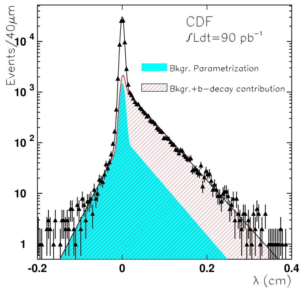
Fig. 13.: The distribution of “pseudo decay length” $\lambda\sim ML_{xy}/p_{T}$ from CDF $B\rightarrow J/\psi\rightarrow\mu\mu$ data. The points are the data, and the curves are the signal and background models. The heavily shaded area is the background; it is asymmetric because of sequential semileptonic $B$ decays in the dimuon sample. The lightly shaded area is the signal contribution, and the unshaded area is from prompt $J/\psi$ mesons. From Ref. [cdfblifetime].

3.4 Characteristics of Signal and Background Events

We have discussed the decay modes of the top quark and the experimental signatures for $t\overline{t}$ production in Sec. 2. We have also outlined how the objects in the final state of a $t\overline{t}$ decay are identified and measured in the two detectors. Here, we shall discuss briefly the kinematic properties of $t\overline{t}$ events in the various decay modes, and how these properties differ for background processes.

In the dilepton channels, the two leptons arise from $W$ boson decays, and therefore tend to be central in pseudorapidity, isolated, and of large transverse momenta. The two $b$-jets also have high transverse energies. There are two high-$p_{T}$ neutrinos, so the missing transverse energy tends to be large as well. The major background for these channels is from the Drell-Yan process, which produces isolated lepton pairs in profusion. Additional jets can arise from initial or final state radiation. The Drell-Yan process yields $ee$ and $\mu\mu$ events directly, while $e\mu$ events can be produced via $\tau\tau$ production and subsequent decay. The $ee$ and $\mu\mu$ events at the $Z$ resonance can be easily eliminated by rejecting events in which the invariant mass of the two leptons is consistent with that of the $Z$ boson, $M_{Z}$. Additional rejection of background is obtained by requiring at least two jets in the final state. In Drell-Yan events, the additional jets are due to gluon radiation; consequently, every additional jet reduces the cross section by a factor of $O(1/\alpha_{s})\sim 6.7$. Requiring a large ${\hbox{$E$\kern-6.00006pt\lower-0.43057pt\hbox{/}}}_{T}$ further reduces the background. In case of $Z\rightarrow\tau\tau\rightarrow(\ell\nu\nu)(\ell\nu\nu)$, the $Z$ boson cannot be reconstructed because of the presence of four unobserved neutrinos in the final state. However, the leptons in these events have much smaller $p_{T}$ than those in $t\overline{t}$ events. So, requiring two high-$p_{T}$ leptons, two or more jets, and large ${\hbox{$E$\kern-6.00006pt\lower-0.43057pt\hbox{/}}}_{T}$ will greatly suppress this background. Other backgrounds which must be considered are diboson production ($WW$, $WZ$, $ZZ$), QCD production of $b\overline{b}$ (with semileptonic decays of the $b$-quarks), and QCD events with jets misidentified as leptons. The distributions of several kinematic quantities for dilepton events are shown in Figs. 14, 15, and 16.

Fig. 14.: Expected distributions for $e\mu$ dilepton events of (a) lepton $p_{T}$ (two entries per event), (b) ${\hbox{$E$\kern-6.00006pt\lower-0.43057pt\hbox{/}}}_{T}$, and (c) lepton $\eta$ (two entries per event). The solid histograms are $t\overline{t}\rightarrow e\mu+X$ signal events (generated with herwig with $m_{t}=175~{}\text{GeV}/c^{2}$ for $p\overline{p}$ collisions at $\sqrt{s}=1.8~{}\text{TeV}$). The dashed histograms are $Z+\text{jets}\rightarrow\tau\tau+\text{jets}\rightarrow e\mu+\text{jets}$ events (also generated with herwig). All histograms are normalized to unity. We require that events have $p_{T}^{\ell}>10~{}\text{GeV}/c$, $\mbox{${\hbox{$E$\kern-6.00006pt\lower-0.43057pt\hbox{/}}}_{T}$}>10~{}\text{GeV}$, and at least two jets with $E_{T}>15~{}\text{GeV}$ and $|\eta|<2.0$.

Fig. 15.: Expected distributions for $e\mu$ events of (a and b) the transverse energies of the two leading jets and (c) the jet $\eta$ (two entries per event). See Fig. 14 for further details.

Fig. 16.: Expected distributions for $e\mu$ events of $H_{T}^{e}\equiv\sum_{\text{jets}}E_{T}^{\text{jet}}+E_{T}^{e1}$. See Fig. 14 for further details.

The dominant background to the lepton+jets channel comes from the production of single $W$ bosons in association with jets. Other backgrounds include false lepton events with mismeasured ${\hbox{$E$\kern-6.00006pt\lower-0.43057pt\hbox{/}}}_{T}$ and/or misidentified $b$-tags, $Wb\overline{b}$ and $Wc\overline{c}$ production, and QCD heavy flavor processes. The distributions of $E_{T}^{\ell}$, $\eta_{\ell}$, and ${\hbox{$E$\kern-6.00006pt\lower-0.43057pt\hbox{/}}}_{T}$ for the signal and for the $W$+jets background are shown in Fig. 17. The major differences between the signal and background processes stem from the number of jets in the event and the event kinematics. Ideally, a lepton+jets $t\overline{t}$ event has four jets, two of which come from $b$-quarks. However, as discussed in Sec. 3.3.1, the number of observed jets can be greater or lesser than four. Therefore, the analyses usually require at least three jets if a $b$-tagged jet is required in the event, and at least four jets otherwise. The jets in background events have lower transverse energies than those in the signal, and are produced over a wider range of $\eta$, as is evident from Fig. 18.

Certain variables describing the overall shape of the event provide powerful means of discriminating lepton+jets signal from background.[d0topprd, d0xsecprl97] One such variable is the aplanarity[barger93] ${\cal{A}}$, defined as $2/3$ times the smallest eigenvalue of the total normalized momentum tensor in the event. This is $0.5$ for spherical events and zero for planar or linear events. Top quark events are expected to be more spherical than radiative QCD processes, and hence to have larger aplanarities. Another useful variable is the sum of the transverse energies of all jets, $H_{T}$. This variable reflects the “temperature” of the interaction; a large $H_{T}$ is a signature of the decay of massive objects.[baer89] Distributions of $H_{T}$ and ${\cal{A}}$ are shown in Fig. 19.

Fig. 17.: Expected distributions for lepton+jets events of (a) lepton $p_{T}$, (b) ${\hbox{$E$\kern-6.00006pt\lower-0.43057pt\hbox{/}}}_{T}$, and (c) lepton $\eta$. The solid histograms are $t\overline{t}$ signal events (generated with herwig with $m_{t}=175~{}\text{GeV}/c^{2}$ for $p\overline{p}$ collisions at $\sqrt{s}=1.8~{}\text{TeV}$). The dashed histograms are $W+\geq 4~{}\text{jets}$ events (generated with vecbos). All histograms are normalized to unity. We require that events have $p_{T}^{\ell}>15~{}\text{GeV}/c$, $\mbox{${\hbox{$E$\kern-6.00006pt\lower-0.43057pt\hbox{/}}}_{T}$}>15~{}\text{GeV}$, and at least four jets with $E_{T}>15~{}\text{GeV}$ and $|\eta|<2.0$.

Fig. 18.: Expected distributions for lepton+jets events of (a–d) the transverse energies of the four leading jets and (e) the jet $\eta$ (four entries per event). See Fig. 17 for further details.

Fig. 19.: Expected distributions for lepton+jets events of (a) $H_{T}$ and (b) aplanarity. See Fig. 17 for further details.

4 Discovery of the Top Quark

The pursuit of the top quark began in earnest in the late 1970s, shortly after the discovery of the $b$-quark at Fermilab.[herb77] Searches at the $e^{+}e^{-}$ colliders PETRA [behrend84] (1979–84, ${\sqrt{s}}=\text{12--46.8}~{}\text{GeV}$), TRISTAN [sagawa88] (1986–90, ${\sqrt{s}}=61.4~{}\text{GeV}$), and SLC [abrams89] and LEP [decamp90] (1989–90, ${\sqrt{s}}\approx M_{Z}$) eventually raised the lower limit on the top quark mass to $45.8~{}\text{GeV}/c^{2}$. (This limit and all others mentioned in this section are $95\%$ confidence level results.) Owing to the pioneering work of S. van der Meer, C. Rubbia, and others, at CERN and elsewhere, high-energy $p\overline{p}$ colliders were developed in the 1980s. The first was the ISR (intersecting storage rings) at CERN[isrppbar]. Next came the S$p\overline{p}$S, also at CERN. With $\sqrt{s}$ up to $630~{}\text{GeV}$, this machine had a beam energy an order of magnitude higher than the ISR. This was followed by the Fermilab Tevatron, with $\sqrt{s}=1.8~{}\text{TeV}$. These machines provided much higher center-of-mass energies, enabling searches for particles with higher masses.

Searches for the top quark at $p\overline{p}$ colliders do not provide direct limits on the mass of the top quark, but rather upper limits on its production cross section. These upper limits can be turned into lower limits on the mass using calculations of the production cross section.

In 1984, the UA1 collaboration reported [arnison84] evidence for the production of top quarks with $m_{t}=40\pm 10~{}~{}\text{GeV}/c^{2}$. In a subsequent analysis, however, with a larger data sample and a more thorough evaluation of backgrounds, the putative signal vanished![albajar88] A limit of $m_{t}>45~{}\text{GeV}/c^{2}$ was inferred from this latter analysis. The UA1 and UA2 experiments continued running through 1989, eventually setting limits of $m_{t}>60~{}\text{GeV}/c^{2}$ and $m_{t}>69~{}\text{GeV}/c^{2}$, respectively.[albajar90] Yet, even as they were in their last stretch, the CDF detector came online at the Fermilab Tevatron in 1988 and started recording $p\overline{p}$ collisions at the unprecedented ${\sqrt{s}}=1.8~{}\text{TeV}$, racing the CERN collaborations for evidence of top quark production with $m_{t}<M_{W}$. The CDF collaboration soon set limits of $m_{t}>77~{}\text{GeV}/c^{2}$ from the $e+\text{jets}$ channel and $m_{t}>72~{}\text{GeV}/c^{2}$ from the $e\mu$ channel.[cdfejets90] Even with a smaller integrated luminosity ($\int\!{\cal L}\,dt=4.4~{}\text{pb}^{-1}$ for CDF vs. $\int\!{\cal L}\,dt=7.5~{}\text{pb}^{-1}$ for UA2), this limit was already better than could be achieved at the S$p\overline{p}$S experiments (because of the higher beam energy of the Tevatron). CDF later extended this analysis, adding the $ee$, $\mu\mu$, and $\mu+\text{jets}$ channels and using soft-lepton $b$-tagging in the lepton+jets channels, arriving at a final limit from the 1988–89 run[cdftopprl92] of $m_{t}>91~{}\text{GeV}/c^{2}$. Given these limits, the CERN experiments were out of the running; the search would continue only at the world’s highest energy collider, the Fermilab Tevatron.

Collider operations at the Tevatron resumed in July, 1992, at which time the CDF detector was joined by the newly-commissioned DØ detector. Collider running continued through 1996, with the Tevatron reaching peak luminosities of over $2\times 10^{31}~{}\text{cm}^{-2}\,\text{s}^{-1}$, a factor of 10 higher than the previous run, and twenty times the design luminosity. The average luminosity for this period was $1.4\times 10^{31}~{}\text{cm}^{-2}\,\text{s}^{-1}$.

Using the data from the first period of running (Run 1a), with $\int\!{\cal L}\,dt=13.5~{}\text{pb}^{-1}$, the DØ experiment soon set a limit of $m_{t}>131~{}\text{GeV}/c^{2}$ using the $ee$, $e\mu$, $e+\text{jets}$, and $\mu+\text{jets}$ channels.[d0topprd, d0xsecprl94] (This limit was later revised downwards to $128~{}\text{GeV}/c^{2}$ because of a recalibration of the luminosity at DØ.) In April 1994, however, the CDF collaboration claimed [cdftopprd94, cdftopprl94] the first evidence for $t\overline{t}$ production. With an integrated luminosity from Run 1a of $19.3~{}\text{pb}^{-1}$, CDF observed twelve candidate events in the dilepton and lepton+jets channels and estimated a $0.26\%$ probability for the background to fluctuate to at least that many events. Assuming that the excess was due to $t\overline{t}$ production, the cross section was measured to be $\sigma_{t\overline{t}}=13.9^{+6.1}_{-4.8}~{}\text{pb}$. Under the same assumption, CDF also measured the top quark mass using the $b$-tagged sample, obtaining a result of $m_{t}=174\pm 10^{+13}_{-12}~{}\text{GeV}/c^{2}$. Meanwhile, the DØ collaboration had reoptimized its analysis to search for high-mass top quarks, with $m_{t}\sim 180~{}\text{GeV}/c^{2}$. Nine candidate events were observed,[d0topprd, d0xsecprl95] compared to $3.8\pm 0.9$ events expected from background. Taking $m_{t}=180~{}\text{GeV}/c^{2}$ yielded a $t\overline{t}$ production cross section of $8.2\pm 5.1~{}\text{pb}$. The chance of the observed signal being an upward fluctuation of the background was calculated to be $2.7\%$; therefore, DØ concluded that the excess was of insufficient statistical significance to demonstrate the existence of the top quark.

Run 1a brought several spectacular $t\overline{t}$ candidate events. In September, 1992, CDF recorded a beautiful $t\overline{t}\rightarrow(W^{+}b)(W^{-}\bar{b})\rightarrow(e^{+}\nu b)(q\bar{q}\bar{b})$ candidate. A display of the SVX tracks in the event is shown in Fig. 20. The event has an isolated electron, large ${\hbox{$E$\kern-6.00006pt\lower-0.43057pt\hbox{/}}}_{T}$, and two jets with clearly identified displaced vertices (indicative of $b$-quark decays). This event will surely find its way into the textbooks as an ideal top-antitop event! A kinematic fit of this single event to the $t\overline{t}$ decay hypothesis yields $m_{t}=170\pm 10~{}\text{GeV}/c^{2}$.

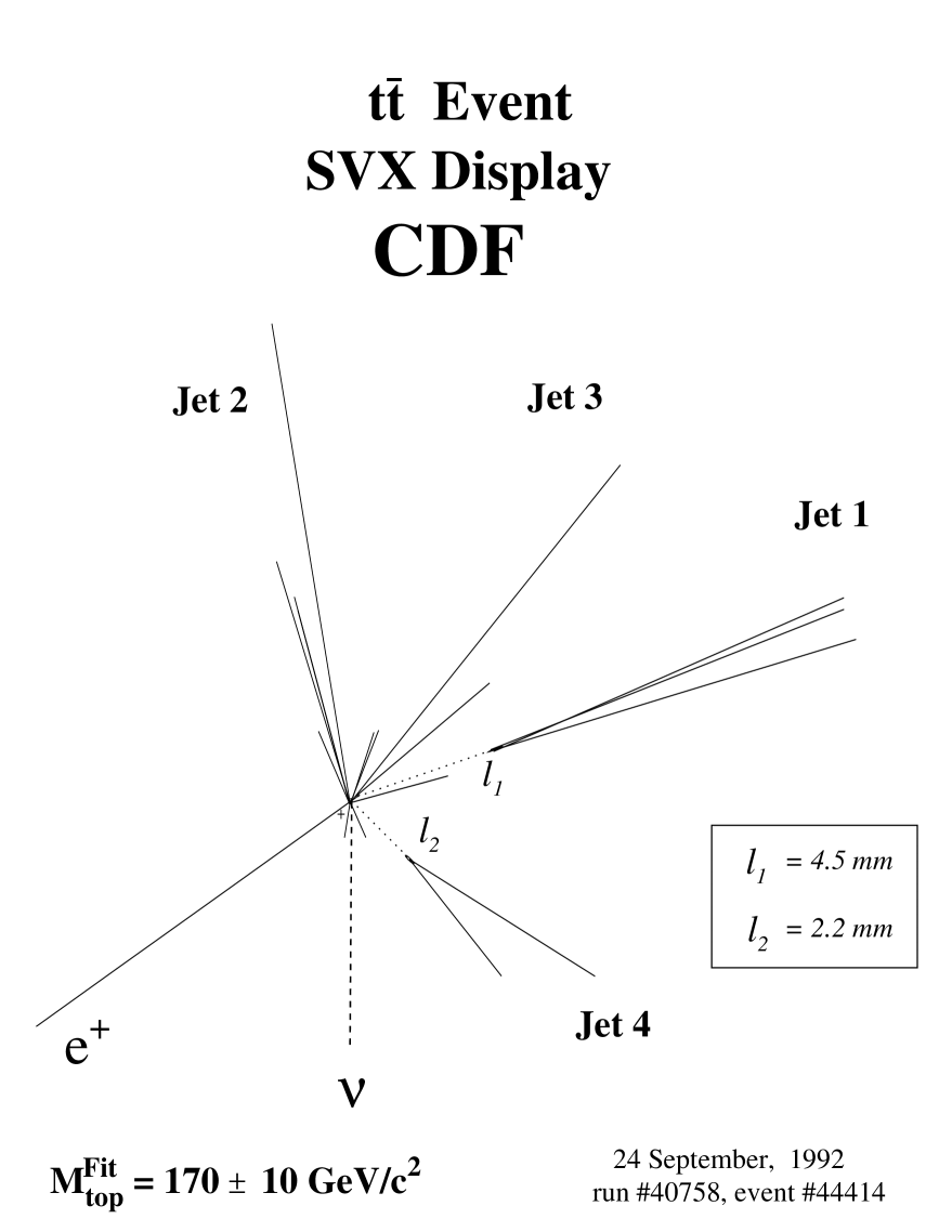
Fig. 20.: A $t\overline{t}\rightarrow e+\text{jets}$ candidate event from the CDF experiment. Jets 1 and 4 are identified by the SVX detector as $b$-quark decays with vertices displaced from the primary event vertex. Jets 2 and 3 could have come from a $W$ boson, and the $e^{+}$ and $\nu$ from the other $W$ boson in the event. From Ref. [kim95].

Another spectacular event is a dilepton ($e\mu$) event recorded by DØ in January, 1993. An event display is shown in Fig. 21. This event has two high-$p_{T}$ leptons ($E_{T}^{e}=98.8~{}\text{GeV}$, $p_{T}^{\mu}=194.6~{}\text{GeV}/c$), large ${\hbox{$E$\kern-6.00006pt\lower-0.43057pt\hbox{/}}}_{T}$ ($100.7~{}\text{GeV}$), and two jets ($E_{T}^{j1}=26.1~{}\text{GeV}$, $E_{T}^{j2}=23.0~{}\text{GeV}$). A multivariate Fisher discriminant analysis [pushpadpf] showed that this event is eighteen times more likely to be a $t\overline{t}$ event than a $(Z\rightarrow\tau\tau)+\text{jets}$ event, and ten times more likely to be $t\overline{t}$ than $WW+\text{jets}$.

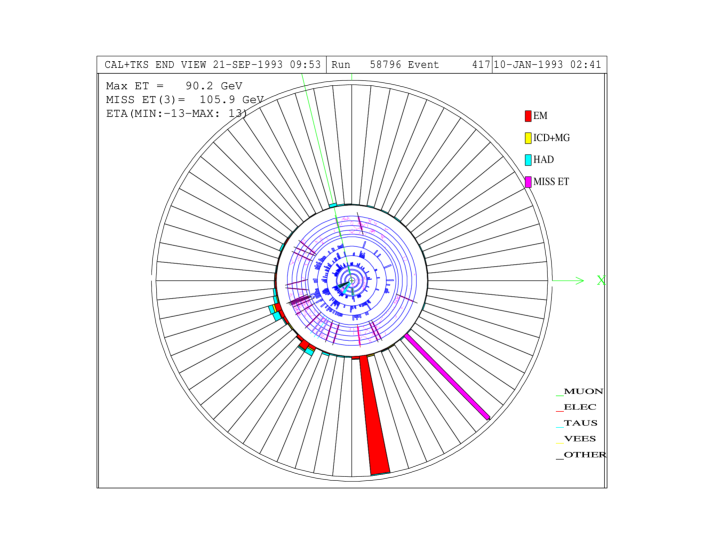
Fig. 21.: An $e\mu+\text{jets}$ candidate event from the DØ experiment. This is an end view of the tracking detectors and the central calorimeter. The muon is shown by the dotted line near the top, the electron is the large EM deposition near the bottom, and the two jets are the smaller depositions at about 7 and 8 o’clock. The ${\hbox{$E$\kern-6.00006pt\lower-0.43057pt\hbox{/}}}_{T}$ is shown by the narrow bar at about 5 o’clock.

Run 1a continued through June, 1993. Over the summer, the accelerator was upgraded, with improvements to the linac and the installation of electrostatic separators. In December, collider operations resumed with Run 1b. By February, 1995, both experiments had quadrupled their data sets, and had observed large excesses of events over background that were fully consistent with the $t\overline{t}$ hypothesis. Finally, on March 2, 1995, the collaborations announced that the long search was over: the top quark had been found.[cdfdiscovery, d0discovery]

CDF, in its $67~{}\text{pb}^{-1}$ data set, observed 37 lepton+jets events with at least one $b$-tag. In this sample, there were 27 SVX $b$-tags, compared to $6.7\pm 2.1$ tags expected from background, and 23 SLT $b$-tags, compared to an expected background of $15.4\pm 2.0$ tags. Six dilepton events were also seen, compared to $1.3\pm 0.3$ events expected from background. The probability for the estimated background to fluctuate to at least the observed number of events was calculated to be $1\times 10^{-6}$, corresponding to a $4.8\sigma$ deviation for a Gaussian distribution. CDF obtained a total $t\overline{t}$ cross section of $6.8^{+3.6}_{-2.4}~{}\text{pb}$, and a mass for the top quark of $m_{t}=176\pm 8~{}\text{(stat)}\pm 10~{}\text{(syst)}~{}\text{GeV}/c^{2}$.

Simultaneously, DØ, using approximately $50~{}~{}\text{pb}^{-1}$ of data, observed 17 events over an estimated background of $3.8\pm 0.6$ events. The probability for the background to fluctuate to at least the measured yield was $2\times 10^{-6}$, equivalent to $4.6\sigma$ for a Gaussian distribution. DØ measured a top quark mass of $m_{t}=199^{+19}_{-21}~{}\text{(stat)}\pm 22~{}\text{(syst)}~{}\text{GeV}/c^{2}$ and a $t\overline{t}$ production cross section of $6.4\pm 2.2~{}\text{pb}$.

5 Measurement of the $t\overline{t}$ Production Cross Section

5.1 General Strategy

Measuring the $p\overline{p}\rightarrow t\overline{t}$ production cross section can be done in several decay modes. These are categorized as either dilepton, lepton+jets, or all-jets, as discussed in Sec. 2. These can be further subdivided based on the lepton flavors in the final states, on whether or not $b$-tags are present, and on the method used for $b$-tagging. For each subchannel, the cross section is given by

$$\sigma_{t\bar{t}}=\frac{(N-B)}{\epsilon\times\int\!{\cal L}\,dt},$$ (18)

where $N$ is the number of observed events, $B$ the estimated background count, $\epsilon$ the total detection efficiency for $t\overline{t}$ events in the subchannel, and $\int\!{\cal L}\,dt$ the integrated luminosity of the data set. The total efficiency $\epsilon$ includes the branching fraction, the geometrical acceptance of the detector, and the efficiencies for trigger selection, identification of leptons and jets, and kinematic selections. For any given set of kinematic selections, the signal efficiency depends on the mass of the top quark; therefore, the measured cross section depends on the assumed value of the mass. For some channels, the background prediction is based on data samples in which there is a small contribution from $t\overline{t}$ production. In such analyses, the measured $t\overline{t}$ cross section is used to correct the background prediction iteratively, until the measured cross section is stable. To obtain a final measurement of the cross section, all channels are combined, taking into account any correlated uncertainties, such as those on integrated luminosity and on the signal and background models.

Both collaborations use the herwig[herwig] Monte Carlo program as the primary model for $t\overline{t}$ events. In addition, CDF uses pythia[pythia] to assess systematic uncertainties due to modeling, while DØ uses isajet.[isajet] The $W$+jets background, which is the principal background in the lepton+jets channels, is modeled using a combination of collider data and simulations based on the vecbos program.[vecbos] The other important background in these channels arises from misidentification of one or more jets as leptons in multijet events. The misidentification rate (called the fake-lepton probability) is obtained from the data, as are the lepton identification efficiencies and the $b$-tag probabilities of the background. Other (smaller) backgrounds are estimated using a combination of Monte Carlo simulations and object identification efficiencies measured from data.

5.2 CDF Analyses

The most up-to-date analyses from CDF use data from Run 1a (1992–93) and Run 1b (1994–95).[cdftoptotau97, cdfxs98, cdfdilep98, cdfalljets] Since Run 1c was short, CDF chose not to trigger on top-like events, but instead used the run to pursue other specialized studies. The total integrated luminosity used in the top analyses is $109\pm 7~{}\text{pb}^{-1}$. If one assumes the predicted $t\overline{t}$ cross section of $5.5~{}\text{pb}$ (at $m_{t}=175~{}\text{GeV}/c^{2}$), about 600 $t\overline{t}$ events should be present in the CDF data. A subset of these data ($\int\!{\cal L}\,dt\sim 67~{}\text{pb}^{-1}$) supported CDF’s observation of the top quark.[cdfdiscovery]

Using the full data set, CDF has updated analyses in the dilepton and lepton+jets/b-tag channels and has performed new analyses in the $\tau$ dilepton ($e\tau$ and $\mu\tau$) and all-jets (all hadronic) channels. The $\tau$ dilepton channels are of special interest because, if charged Higgs bosons $H^{\pm}$ with $m_{H}^{\pm}<m_{t}$ exist, they could produce an excess of events in these modes via the decay chain $t\rightarrow H^{+}b\rightarrow\tau^{+}\nu_{\tau}b$.

The all-jets final state accounts for $44\%$ of all $t\overline{t}$ events. It is therefore both important and interesting to test this key prediction through an independent observation of signal in this channel.

CDF calculates $\sigma_{t\overline{t}}$ assuming $m_{t}=175~{}\text{GeV}/c^{2}$, while DØ uses $m_{t}=172~{}\text{GeV}/c^{2}$. This corresponds to a typical difference of $\approx 0.3$ pb in extracted cross sections, due to the dependence of the efficiency on mass.

5.2.1 Dilepton Channels

We discuss first the analyses in the “standard” dilepton channels, $ee$, $e\mu$, and $\mu\mu$,[cdfdilep98] and leave dilepton channels with identified $\tau$ leptons for later.

The initial event selection in the standard dilepton analyses requires the presence of two oppositely charged high-$p_{T}$ leptons ($e$ or $\mu$), two or more jets as expected from the $b$-quarks, and large ${\hbox{$E$\kern-6.00006pt\lower-0.43057pt\hbox{/}}}_{T}$ as the signature for the neutrinos. The kinematic selection criteria are shown in Table 5. Since both leptons in dilepton $t\overline{t}$ events come from $W$ boson decays, at least one of the two leptons is required to be isolated. The criterion for lepton isolation is that the transverse energy in the calorimeter in a cone of $R=0.4$ around the lepton be less than $10\%$ of the lepton’s $E_{T}$ (or $p_{T}$). The dominant background to the $ee$ and $\mu\mu$ channels comes from $Z(\rightarrow\ell\ell)+\text{jets}$. This is largely eliminated by rejecting events with a dilepton invariant mass $M_{\ell\ell}$ within a narrow window about the $Z$ boson mass, that is, with $|M_{\ell\ell}-M_{Z}|<15~{}\text{GeV}/c^{2}$. Events containing an isolated photon with $E_{T}>10~{}\text{GeV}$ consistent with a radiative decay of a $Z$ boson are removed. The requirement on the ${\hbox{$E$\kern-6.00006pt\lower-0.43057pt\hbox{/}}}_{T}$ is tightened (to $\mbox{${\hbox{$E$\kern-6.00006pt\lower-0.43057pt\hbox{/}}}_{T}$}>50~{}\text{GeV}$) when the ${\hbox{$E$\kern-6.00006pt\lower-0.43057pt\hbox{/}}}_{T}$ vector is nearly collinear with either a lepton or a jet ($\Delta\phi(\mbox{${\hbox{$E$\kern-6.00006pt\lower-0.43057pt\hbox{/}}}_{T}$},\text{$\ell$ or jet})<20^{\circ}$). This suppresses backgrounds from $Z\rightarrow\tau\tau$, where the two $\tau$ leptons (and hence their decay products) are spatially close when the decaying $Z$ boson has high momentum, and background from the Drell-Yan continuum where ${\hbox{$E$\kern-6.00006pt\lower-0.43057pt\hbox{/}}}_{T}$ arises from mismeasurements of jet or lepton energies. The latter process has a very large cross section, and therefore is an important source of background. The distribution of $\Delta\phi($${\hbox{$E$\kern-6.00006pt\lower-0.43057pt\hbox{/}}}_{T}$$,\text{$\ell$ or jet})$ vs. ${\hbox{$E$\kern-6.00006pt\lower-0.43057pt\hbox{/}}}_{T}$ is shown in Fig. 22 for events that pass all but the final selection criterion. The expected distribution for $t\overline{t}$ events, calculated with herwig assuming $m_{t}=175~{}\text{GeV}/c^{2}$, is superimposed for comparison. Nine events — seven $e\mu$, one $ee$, and one $\mu\mu$ — survive all the requirements. The distribution of $H_{T}^{\text{all}}$ ($\equiv p_{T}^{\ell 1}+p_{T}^{\ell 2}+\mbox{${\hbox{$E$\kern-6.00006pt\lower-0.43057pt\hbox{/}}}_{T}$}+E_{T}^{\text{jet1}}+E_{T}^{\text{jet2}}$) for candidate events is compared to expectations for signal and background in Fig. 23.

Table 5.: Basic kinematic requirements in various channels in the CDF cross section measurements.

	Standard Dilepton	$\tau$-Dilepton	$\ell+\text{jets}$/$b$-tag	All jets
	($ee$, $e\mu$, $\mu\mu$)	($e\tau$, $\mu\tau$)
Lepton $p_{T}(\text{GeV}/c)$	$>20$	$p_{T}^{\tau}>15$	$>20$	—
		$p_{T}^{e,\mu}>20$
Lepton $|\eta|$	$<1.0$	$|\eta^{\tau}|<1.2$	$<1.0$	—
		$|\eta^{e,\mu}|<1.0$
${\hbox{$E$\kern-6.00006pt\lower-0.43057pt\hbox{/}}}_{T}$ (GeV)	$>25$	—	$>20$	—
$S_{\mbox{${\hbox{$E$\kern-4.20004pt\lower-0.3014pt\hbox{/}}}_{T}$}}$ ($\text{GeV}^{1/2}$)	—	$>3$	—	—
Jet $E_{T}$ (GeV)	$>10$	$>10$	$>15$	$>15$
Jet $|\eta|$	$<2.0$	$<2.0$	$<2.0$	$<2.0$
Number of jets	$\geq 2$	$\geq 2$	$\geq 3$	$\geq 5$
$H_{T}$ (GeV)	—	—	—	$>300$
$H_{T}^{\text{all}}$(GeV)	—	$>180$	—	—

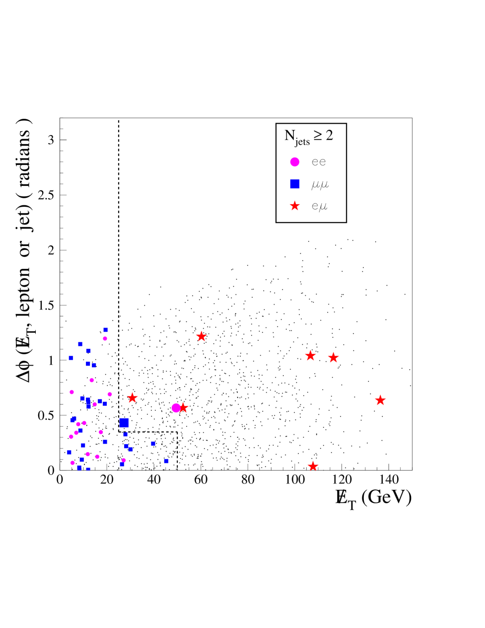
Fig. 22.: The azimuthal angle $\Delta\phi$ between the ${\hbox{$E$\kern-6.00006pt\lower-0.43057pt\hbox{/}}}_{T}$ vector and the nearest lepton or jet vs. ${\hbox{$E$\kern-6.00006pt\lower-0.43057pt\hbox{/}}}_{T}$ in CDF dilepton events. The small points show the distribution expected from $t\overline{t}$ signal with $m_{t}=175~{}\text{GeV}/c^{2}$. The larger symbols represent data. The dashed line shows the cuts on ${\hbox{$E$\kern-6.00006pt\lower-0.43057pt\hbox{/}}}_{T}$. From Ref.[cdfdilep98].

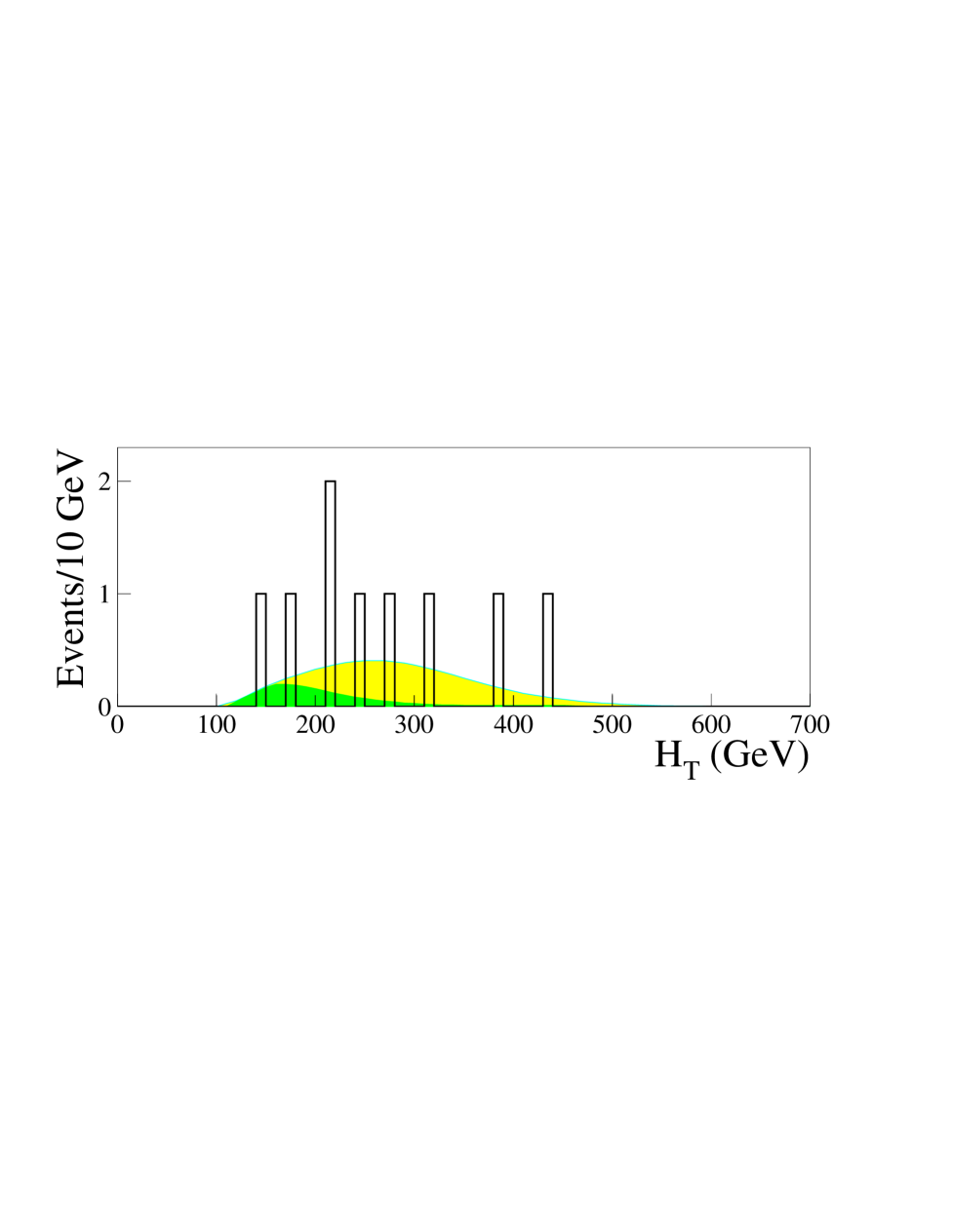
Fig. 23.: Comparison of $H_{T}^{\text{all}}$ for the CDF dilepton candidate events (histogram) with the expectation for $t\overline{t}$ production ($m_{t}=175~{}\text{GeV}/c^{2}$) plus background (lighter shaded area). The darker shaded area represents background alone. From Ref.[cdfdilep98].

The estimates of the backgrounds from various sources are listed in Table 6. After the initial event selection, Drell-Yan ($Z/\gamma^{*}\rightarrow ee,\mu\mu$) production continues to be the major background for the $ee$ and $\mu\mu$ channels. The $e\mu$ channel, the cleanest of the dilepton channels, has background mainly from decays of $W$ boson pairs ($WW$) and $Z\rightarrow\tau\tau$. In all cases, additional jets can arise from gluon radiation, and ${\hbox{$E$\kern-6.00006pt\lower-0.43057pt\hbox{/}}}_{T}$ from either neutrinos or mismeasurement of energies. CDF also estimates the background from false signatures due to particle misidentification, such as a jet or a track faking one of the leptons, or overestimated ${\hbox{$E$\kern-6.00006pt\lower-0.43057pt\hbox{/}}}_{T}$ due to mismeasured muon momenta. The backgrounds from Drell-Yan production, fake leptons, and mismeasured tracks are estimated from the data. Other backgrounds are calculated using Monte Carlo simulations, which use lepton identification efficiencies estimated from data.

Table 6.: Expected backgrounds to the standard dilepton channels in the CDF data, corresponding to $\int\!{\cal L}\,dt=109\pm 7~{}\text{pb}^{-1}$. From Ref. [cdfdilep98].

Background type	Expected Number of events
	(All dilepton channels)
Drell-Yan	$0.61\pm 0.30$
$Z\rightarrow\tau\tau$	$0.59\pm 0.14$
Fake leptons	$0.37\pm 0.23$
$WW$	$0.36\pm 0.11$
Mismeasured muon tracks	$0.30\pm 0.30$
QCD $b\overline{b}$	$0.05\pm 0.03$
Other (radiative $Z$, $W\overline{b}$, $WZ$, $ZZ$)	$0.10\pm 0.10$
Total	$2.40\pm 0.50$

For the acceptance of $t\overline{t}$ events, CDF takes the average of the results from herwig and pythia. The lepton identification efficiencies are measured to be 91% for muons and 83% for electrons, using $Z\rightarrow\ell^{+}\ell^{-}$ data. (These efficiencies do not include the geometric acceptance of the detector or the isolation cuts.) The overall efficiency for detection of $t\overline{t}$ events (including the branching ratio) is estimated to be $\epsilon=(0.74\pm 0.08)\%$ for $m_{t}=175~{}\text{GeV}/c^{2}$. The uncertainty in the efficiency reflects uncertainties in event modeling (estimated from the differences between herwig and pythia) and in the simulation of the detector. Assuming a $t\overline{t}$ production cross section of $5.5~{}\text{pb}$, CDF expects to see a total of 4.4 $t\overline{t}$ events in the standard dilepton channels, of which $(58\pm 2)\%$ are expected to be $e\mu$, $(27\pm 1)\%$ $\mu\mu$, and $(15\pm 1)\%$ $ee$. Both charged leptons directly come from $W$ boson decays in $(86\pm 2)\%$ of the observed dilepton $t\overline{t}$ events. In the remaining events, one of the leptons comes from the decay chain $W\rightarrow\tau\rightarrow e/\mu$. The total $t\overline{t}$ acceptance increases by 35% as $m_{t}$ increases from 150 to $200~{}\text{GeV}/c^{2}$.

With nine dilepton events in the data sample, an estimated background of $2.4\pm 0.5$ events, and an overall $t\overline{t}$ efficiency of $(0.74\pm 0.08)\%$, the cross section for $t\overline{t}$ production for $m_{t}=175~{}\text{GeV}/c^{2}$ is found to be $8.2_{-3.4}^{+4.4}~{}\text{pb}$. Of the nine candidate events, four have one jet tagged as a $b$-jet by the SVX algorithm; of these four, two are also tagged by the SLT method. If all nine candidates are assumed to be from background processes, the number of expected $b$-tagged jets is only $0.7\pm 0.2$.

CDF also searches for $t\overline{t}$ events in the $e\tau$ and $\mu\tau$ decay channels.[cdftoptotau97] The total branching ratio for these channels is $4/81$, the same as for all the standard dilepton modes (see Sec. 2.2). This could, in principle, double the efficiency for dilepton modes. That is not the case, however, since only hadronic decays of the $\tau$ are used (branching fraction $\approx 64\%$: $50\%$ one-prong and $14\%$ three-prong decays), and the identification of $\tau$ leptons is far less efficient than of electrons or muons.

Recall from Sec. 3.3.4 that CDF uses two different $\tau$ identification algorithms, one “track-based” and the other “calorimeter-based.” Separate cross section analyses are performed for each of these selections, starting from samples containing events with $\tau$ candidates along with oppositely charged leptons satisfying the kinematic cuts summarized in Table 5. Each event must also contain at least two jets (since we expect two $b$-quarks) with $E_{T}>10~{}\text{GeV}$ and $|\eta|<2.0$, and have significant ${\hbox{$E$\kern-6.00006pt\lower-0.43057pt\hbox{/}}}_{T}$ due to the unobserved neutrinos. Instead of directly applying a cut on ${\hbox{$E$\kern-6.00006pt\lower-0.43057pt\hbox{/}}}_{T}$, CDF applies a cut on the ${\hbox{$E$\kern-6.00006pt\lower-0.43057pt\hbox{/}}}_{T}$ significance, defined as $S_{\mbox{${\hbox{$E$\kern-4.20004pt\lower-0.3014pt\hbox{/}}}_{T}$}}=\mbox{${\hbox{$E$\kern-6.00006pt\lower-0.43057pt\hbox{/}}}_{T}$}/\sqrt{\sum E_{T}}$ for $e\tau$ events, and $S_{\mbox{${\hbox{$E$\kern-4.20004pt\lower-0.3014pt\hbox{/}}}_{T}$}}=\mbox{${\hbox{$E$\kern-6.00006pt\lower-0.43057pt\hbox{/}}}_{T}$}/\sqrt{\sum E_{T}+p_{T}^{\mu}}$ for $\mu\tau$ events. Here $\sum E_{T}$ is the scalar sum of the transverse energies measured in the calorimeter and provides a measure of the ${\hbox{$E$\kern-6.00006pt\lower-0.43057pt\hbox{/}}}_{T}$ resolution. The requirement on the ${\hbox{$E$\kern-6.00006pt\lower-0.43057pt\hbox{/}}}_{T}$ significance is $S_{\mbox{${\hbox{$E$\kern-4.20004pt\lower-0.3014pt\hbox{/}}}_{T}$}}>3~{}\text{GeV}^{1/2}$. The distributions of $S_{\mbox{${\hbox{$E$\kern-4.20004pt\lower-0.3014pt\hbox{/}}}_{T}$}}$ vs. ${\hbox{$E$\kern-6.00006pt\lower-0.43057pt\hbox{/}}}_{T}$ for the $e\tau$ and $\mu\tau$ data samples as well as for $t\overline{t}$ Monte Carlo events are shown in Fig. 24. A cut $H_{T}^{\text{all}}>180~{}\text{GeV}$ is also imposed (where $H_{T}^{\text{all}}\equiv p_{T}^{\ell}+p_{T}^{\tau}+\mbox{${\hbox{$E$\kern-6.00006pt\lower-0.43057pt\hbox{/}}}_{T}$}\ +\sum_{\text{jets}}E_{T}^{\text{jet}}$, $\ell=e$ or $\mu$). Using either $\tau$ identification method, the same four events are left after all cuts, two $e\tau$ and two $\mu\tau$ (shown as stars in Fig. 24). Three of these events are $b$-tagged, and one has an SLT-SLT double-tag.

Fig. 24.: The distribution of $S_{\mbox{${\hbox{$E$\kern-4.20004pt\lower-0.3014pt\hbox{/}}}_{T}$}}$ vs. ${\hbox{$E$\kern-6.00006pt\lower-0.43057pt\hbox{/}}}_{T}$ for CDF events with a primary lepton and a $\tau$ candidate. Three of the four final candidate events (stars) have $b$-tagged jets. From Ref. [cdftoptotau97].

The $\tau$ identification and signal efficiencies are estimated using pythia $t\overline{t}$ events decayed with the tauola package,[tauola] which properly treats the $\tau$ polarization. The $\tau$ identification is cross checked using a data sample enriched in $W\rightarrow\tau\nu_{\tau}$ decays (see Fig. 11). Of all the selected one-prong events, $19\%$ and $38\%$ are found only by the track-based and calorimeter-based techniques, respectively, and $43\%$ by both. The overall signal efficiency is estimated to be $\epsilon=(0.085\pm 0.010~{}\text{(stat)}\pm 0.012~{}\text{(syst)})\%$ for the track-based analysis, and $\epsilon=(0.134\pm 0.013~{}\text{(stat)}\pm 0.019~{}\text{(syst)})\%$ for the calorimeter-based analysis.

The systematic uncertainty is dominated by uncertainties in identification efficiencies for the $\tau$ (6%) and $e/\mu$ (7%) and in the hadronic energy scale of the calorimeter (5%). The uncertainty in the top quark mass contributes another 6%. If one uses the $t\overline{t}$ production cross section of $\sigma_{t\overline{t}}=7.6^{+1.8}_{-1.5}~{}\text{pb}$, measured by CDF from other decay channels, one expects $0.7\pm 0.2~{}\text{(stat)}\pm 0.1~{}\text{(syst)}$ and $1.1\pm 0.3~{}\text{(stat)}\pm 0.2~{}\text{(syst)}$ $t\overline{t}$ events in the track-based and calorimeter-based analyses, respectively. So, if the top quark decays as predicted by the Standard Model, these channels are not expected to improve significantly the acceptance for signal.

The primary background in the $e\tau$ and $\mu\tau$ decay channels comes from $Z/\gamma^{*}\rightarrow\tau^{+}\tau^{-}+\text{jets}$ events, where one $\tau$ decays leptonically and the other hadronically. The other backgrounds include $WW$ and $WZ$ production and “fake $\tau$’s” in $W+\text{jets}$ events, where a jet is misidentified as a $\tau$. The fake $\tau$ background is calculated by weighting the $E_{T}$ spectrum of all jets that could be misidentified as $\tau$’s in the $W+\geq 3~{}\text{jets}$ sample by the fake rate, determined by applying the $\tau$ selection criteria to a multijet event sample. The background estimates are shown in Table 7. The total background for events with $N_{\text{jet}}\geq 2$ is estimated to be $1.28\pm 0.29$ events for the track-based selection and $2.50\pm 0.43$ events for the calorimeter-based selection. The measured $t\overline{t}$ production cross sections, based on the four events observed, are $\sigma_{t\overline{t}}=29.1_{-18.4}^{+26.3}~{}\text{(stat)}\pm 4.7~{}\text{(syst)}~{}\text{pb}$ for the track-based selection and $\sigma_{t\overline{t}}=10.2_{-10.2}^{+16.3}~{}\text{(stat)}\pm 1.6~{}\text{(syst)}~{}\text{pb}$ for the calorimeter-based selection. Unfortunately, because of their large uncertainties, these measurements do not improve the precision of the overall cross section measurement. But the analysis is important because non-standard decays of top, specifically $t\rightarrow H^{+}b$ with $H^{+}\rightarrow\tau^{+}\nu_{\tau}$, could have produced an excess above the Standard Model prediction. No significant excess is evident.

Table 7.: Numbers of events expected and observed for the CDF $\tau$-dilepton analyses. The one-jet columns are background dominated; the columns with two or more jets correspond to the signal region. From Ref. [cdftoptotau97].

Selection	Track-based		Calorimeter-based
$N_{\text{jet}}\geq 10~{}\text{GeV}$	1	$\geq 2$	1	$\geq 2$
$\tau$ fakes	$0.14\pm 0.01$	$0.25\pm 0.02$	$0.47\pm 0.03$	$0.78\pm 0.04$
$Z/\gamma\rightarrow\tau^{+}\tau^{-}$	$0.22\pm 0.12$	$0.89\pm 0.28$	$0.54\pm 0.16$	$1.48\pm 0.38$
$WW$, $WZ$	$0.14\pm 0.06$	$0.14\pm 0.08$	$0.20\pm 0.09$	$0.24\pm 0.10$
Total Background	$0.50\pm 0.14$	$1.28\pm 0.29$	$1.21\pm 0.28$	$2.50\pm 0.43$
Expected from $t\overline{t}$	$0.08\pm 0.02$	$0.70\pm 0.30$	$0.13\pm 0.03$	$1.10\pm 0.40$
Observed events	1	4	0	4

5.2.2 Lepton+Jets Channels

To measure the $t\overline{t}$ production cross section in the lepton+jets channels,[cdfxs98] CDF accumulated data using inclusive electron and muon triggers that required $p_{T}^{\ell}>18~{}\text{GeV}/c$. A ${\hbox{$E$\kern-6.00006pt\lower-0.43057pt\hbox{/}}}_{T}$ trigger was used to compensate for small inefficiencies in the lepton triggers.

The signal in this channel, $t\overline{t}\rightarrow(W^{+}b)(W^{-}{\overline{b}})\rightarrow(\ell\nu b)(q\overline{q}^{\prime}\overline{b})$, is subject to a large background from $W$+jets production. Since it is hard to identify $W$ bosons that decay hadronically, these $t\overline{t}$ events comprise a subset of the $W(\rightarrow\ell\nu)+\text{jets}$ sample. This sample is used for systematic studies of the background involving a $W$ boson, as well as for extracting the signal.

The initial data set consists of high-$p_{T}$ inclusive lepton events that contain a central ($|\eta|<1.0$) isolated electron or muon with $p_{T}>20~{}\text{GeV}/c$. The lepton isolation $I$ is defined as the ratio of the transverse energy in a cone of $R=0.4$ around the lepton (excluding the lepton energy) to the $p_{T}$ of the lepton; the analysis requires $I<0.1$. Events consistent with $Z\rightarrow\ell\ell$ or $Z\rightarrow\ell\ell\gamma$ are rejected, as in the dilepton analysis. From this inclusive lepton sample, events with $\mbox{${\hbox{$E$\kern-6.00006pt\lower-0.43057pt\hbox{/}}}_{T}$}>20~{}\text{GeV}$ are selected for further study. Events that pass the dilepton selection criteria are removed in order to keep the two samples disjoint. This gives an inclusive sample of $W+\text{jets}$ events.

Nominally, one expects to observe four jets per $t\overline{t}$ event in the lepton+jets channels. But, as discussed in Sec. 3.3.1, the number of jets may be larger or smaller than this. Therefore, the analysis requires a minimum of only three jets. The kinematic selection criteria are summarized in Table 5.

CDF uses both the SVX and SLT algorithms for $b$-tagging, with efficiencies of $(39\pm 3)\%$ and $(18\pm 2)\%$, respectively, for tagging at least one $b$-quark in a $t\overline{t}$ event with at least three jets. These tagging efficiencies are estimated from a $t\overline{t}$ Monte Carlo simulation. After all cuts are applied, the $W+\geq 3~{}\text{jets}$ sample contains 34 SVX-tagged events containing a total of 42 SVX-tagged jets, and 40 SLT-tagged events with 44 SLT-tagged jets. Of these events, 11 are $b$-tagged by both algorithms.

The primary background is from $W$+heavy flavor production processes. For the SVX-tagged sample, CDF estimates this background by using vecbos and herwig to predict, as a function of jet multiplicity, the fraction of $W+\text{jets}$ events that contain heavy flavor. This is then combined with the tag probability and applied to the observed $W+\text{jets}$ events. Backgrounds from processes that do not produce a $W$ boson are calculated from the data by measuring the tagging rate in a sample with low ${\hbox{$E$\kern-6.00006pt\lower-0.43057pt\hbox{/}}}_{T}$ and without isolated leptons, where there are few $W$ bosons. This is then used to predict the amount of contamination in the signal region. The background due to mistags can be found by assuming that the distribution of decay lengths from this source is symmetric around zero. CDF measures the negative half of this distribution from jet data and uses that to predict the number of events fluctuating above the cut. The background expected from single top production is also calculated, using the latest theoretical cross sections[heinson97b] and efficiencies derived from Monte Carlo simulations. Additional small backgrounds from $WW$, $WZ$, and $Z\rightarrow\tau\tau$ processes are calculated from Monte Carlo simulations.

For the SLT-tagged sample, the background is mainly from $W+\text{jets}$ events with fake leptons, $K$ decays in flight, electrons from photon conversions, and events containing heavy flavor jets ($Wb\overline{b}$, $Wc\overline{c}$). These backgrounds are calculated from jet data by measuring the tag probability per track as a function of the track $p_{T}$. These tag probabilities are then applied to the tracks in the $W+\text{jets}$ events to estimate the background from these sources.

The signal efficiency, which includes the trigger, tagging and lepton identification efficiencies, kinematic and geometric acceptances, and the branching fraction, is estimated using a combination of data and Monte Carlo events. For $m_{t}=175~{}\text{GeV}/c^{2}$, the overall efficiency is $(3.7\pm 0.3)\%$ with SVX-tagging and $(1.7\pm 0.3)\%$ with SLT-tagging.

The main systematic uncertainties arise from the jet energy scale ($\pm 5\%$), modeling of initial and final state gluon radiation $(\pm 2\%$ and $\pm 5\%$, respectively), Monte Carlo generators ($\pm 5\%$), detector resolution effects ($\pm 2\%$), and the instantaneous luminosity ($\pm 1\%$).

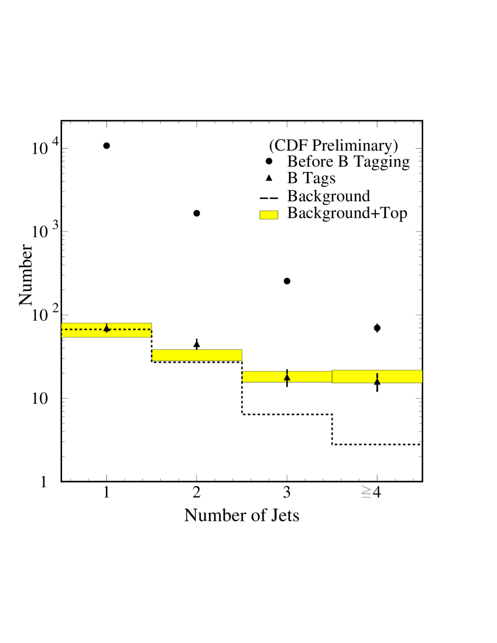
Fig. 25.: The CDF jet multiplicity distribution of SVX-tagged lepton+jets events. Note the clear excess above background for events with three or more jets. From Ref. [gerdes97].

The results of the analysis are summarized in Table 8; the SVX-tagged results are also displayed in Fig. 25. Note that the SVX-based analysis achieves a signal to background ratio about five times better than the SLT-based analysis, demonstrating the clear advantage of $b$-tagging with a silicon vertex detector. Finally, for $m_{t}=175~{}\text{GeV}/c^{2}$, CDF obtains a cross section of $6.2^{+2.1}_{-1.7}~{}\text{pb}$ using the SVX analysis, and $9.2^{+4.3}_{-3.6}~{}\text{pb}$ using the SLT analysis.

Table 8.: Summary of CDF acceptance factors, event yields, backgrounds, and measured cross sections for each analysis channel, for $m_{t}=175~{}\text{GeV}/c^{2}$.

	Dilepton	Lepton+Jets		All-Jets
		SVX	SLT	SVX	2 SVX
$\epsilon_{\text{total}}$	$0.0074\pm 0.0008$	$0.037\pm 0.005$	$0.017\pm 0.0003$	$0.044\pm 0.010$	$0.030\pm 0.010$
Obs. Events	9	34	40	187	157
Background	$2.4\pm 0.5$	$9.2\pm 1.5$	$22.6\pm 2.8$	$142\pm 12$	$120\pm 18$
Expected $t\overline{t}$	4.4	31.0	14.3
$\sigma_{t\overline{t}}$ (pb)	$8.2_{-3.4}^{+4.4}$	$6.2_{-1.7}^{+2.1}$	$9.2_{-3.6}^{+4.3}$	$9.6_{-3.6}^{+4.4}$	$11.5_{-7.0}^{+7.7}$

5.2.3 All-Jets Channel

The all-jets channel has the advantage of having a large branching fraction ($\approx 44$%) and a fully reconstructible final state (since no high-$p_{T}$ neutrinos are present). However, it is subject to an overwhelming background from QCD multijet production, with about one thousand times the rate of $t\overline{t}$ production. But, by requiring large transverse energy in the final state as well as the presence of $b$-quarks, the multijet background can be reduced to manageable levels.

CDF recently reported [cdfalljets] the first observation of $t\overline{t}$ decays in the all-jets channel (referred to as the all hadronic channel by CDF). The collaboration performs two analyses, which require either a single or a double $b$-tag, and, in both cases, finds an excess relative to the estimated background.

The data sample was collected using a special multijet online trigger, specifically developed for $t\overline{t}$ decays into the all-jets final state. This trigger requires four or more clusters of contiguous towers in the calorimeter, each with $E_{T}\geq 15~{}\text{GeV}$ and a total transverse energy of $\sum E_{T}^{\text{jet}}\geq 125~{}\text{GeV}$. Offline, jets are reconstructed using a cone algorithm with $R=0.4$, and jet energy corrections are applied (see Sec. 3.3.1). Selecting events with five or more jets and requiring $\sum E_{T}\geq 300~{}\text{GeV}$ yields 21,840 events. Events with high-$p_{T}$ electrons and muons (which would appear in the dilepton and lepton+jets channels) are removed. After this selection, the QCD background still dominates $t\overline{t}$ production by a factor of about 110. But when one demands at least one SVX $b$-tag, the signal to background ratio increases to $S/B\approx 1/20$, in a sample of $1596$ events. Thereafter, two approaches (referred to as Techniques I and II) are used to further reduce background.

In Technique I, two new variables are introduced that together prove decisive in achieving the final $S/B$ ratio of $\approx 1/4$:

• The centrality $C=H_{T}/\sqrt{\hat{s}}$, where $\sqrt{\hat{s}}$ is the invariant mass of the multijet system.

• The aplanarity ${\cal{A}}$, computed from the jet momenta.

The following cuts are then made on these variables:

• $C>0.75$.

• ${\cal{A}}>-0.0025H_{T3}+0.54$; ($H_{T3}=H_{T}-E_{T}^{\text{jet}1}-E_{T}^{\text{jet}2}$).

The motivation for the first cut is the observation that the jets from $t\overline{t}$ decay are more central than those from QCD production (see Sec. 2). The DØ collaboration uses a similar variable, except that the $H_{T}$ is divided by the sum of the jet energies (see Sec. 5.3). The second cut provides a more optimal way to separate signal from background than that afforded by independent cuts on the aplanarity and $H_{T}$. (Cuts of this kind in the (${\cal{A}},H_{T}$)-plane were first used by DØ.[pushpadpf, pushpapbarp])

After all cuts, 187 events containing 222 $b$-tags remain. This is a statistically significant excess over the estimated background of $164.8\pm 10.8$ $b$-tags. The background is largely from QCD production of heavy quark pairs and from fake $b$-tags. The probability for finding a $b$-tag in a multijet sample, using the SVX algorithm, is parameterized in terms of the jet $E_{T}$, $\eta$ and track multiplicity, and the event aplanarity. To estimate the background, each multijet event is weighted by its tag probability. The sum of these weights, for the multijet events that pass all cuts, gives the background estimate. But, because the multijet sample contains $t\overline{t}$ events, the background estimate must be corrected to account for the $t\overline{t}$ contribution in the multijet sample. This procedure is done iteratively. The tag probabilities are cross checked by comparing predicted $b$-tagged distributions with those observed, using an independent multijet sample.

The uncertainty of the background estimate is dominated by systematics arising from the dependence of the tag probability on the run conditions (such as instantaneous luminosity), the event shape, and kinematics. In Table 8 we summarize the event yields and the background estimates for $N_{\text{jets}}\geq 5$. CDF estimates the probability of the background fluctuating to at least the number of observed $b$-tags as ${\cal P}=1.5\times 10^{-3}$, corresponding to three standard deviations for a Gaussian distribution.

From the number of tagged events and the background estimate, corrected for the $t\overline{t}$ content, CDF extracts the number of $t\overline{t}$ candidates to be $10.4\pm 6.0$ for Run 1a data and $34.7\pm 16.1$ for Run 1b data. The total signal efficiency is estimated to be $(9.9\pm 1.6)\%$ for $m_{t}=175~{}~{}\text{GeV}/c^{2}$. The uncertainty in the efficiency is largely due to systematic uncertainties in the jet energy scale (9%), in modeling of fragmentation (9%) and gluon radiation (11%). The $b$-tagging efficiencies for the two data periods are $(38\pm 11)\%$ and $(46\pm 5)\%$, respectively. The $t\overline{t}$ cross section is measured to be $\sigma_{t\overline{t}}=9.6\pm 2.9~{}\text{(stat)}^{+3.3}_{-2.1}~{}\text{(syst)}~{}\text{pb}$.

In Technique II, two or more $b$-tags are required in each event. Requiring the second $b$-tag significantly reduces the acceptance. Most of this is recovered, however, by removing the centrality and aplanarity requirements. CDF observes 157 such events with $\geq 5~{}\text{jets}$, while background from QCD heavy flavor production and fake double tags is predicted to be $122.7\pm 13.4$ events. The number of signal events is extracted from a likelihood fit of a sum of contributions from fake double tags, QCD heavy flavor background, and $t\overline{t}$ signal, to the observed number of events as a function of jet multiplicity. The number of $t\overline{t}$ candidates is found to be $5.9\pm 3.9$ for Run 1a and $31.6\pm 16.4$ for Run 1b. The corresponding numbers of background events are $21.1\pm 4.5$ and $98.4\pm 17.3$. The detection efficiency before tagging for $t\overline{t}$ events is $(26.3\pm 4.5)\%$ for $m_{t}=175~{}\text{GeV}/c^{2}$. The estimated efficiencies for tagging $\geq 2$ heavy flavor jets are $(7\pm 6)\%$ and $(12\pm 2)\%$ for the two data-taking periods. The cross section is $\sigma_{t\overline{t}}=11.5\pm 5.0~{}\text{(stat)}^{+5.9}_{-5.0}~{}\text{(syst)}~{}\text{pb}$. The probability for the background to produce at least the observed excess is ${\cal P}=2.5\times 10^{-2}$, which corresponds to two standard deviations for a Gaussian distribution.

CDF combines the results from the two techniques to calculate an overall cross section, taking into account the correlations in the efficiencies for the two techniques as well as the overlap between the two data samples (for which 34 events are in common). The correlation coefficient between the two techniques is estimated to be $\rho=0.34\pm 0.13$. For $m_{t}=175~{}~{}\text{GeV}/c^{2}$, the combined measurement is $\sigma_{t\overline{t}}=10.1\pm 1.9~{}\text{(stat)}^{+4.1}_{-3.1}~{}\text{(syst)}~{}\text{pb}$.

5.3 DØ Analyses

The DØ collaboration has used its full Run 1 data set of $125\pm 7~{}\text{pb}^{-1}$ to measure the $t\overline{t}$ production cross section.[d0xsecprl97] Here, we review the DØ measurements for the various decay channels. These cross sections are calculated for $m_{t}=172.1~{}\text{GeV}/c^{2}$.[d0ljtopmassprd]

5.3.1 Dilepton Channels

DØ used the standard dilepton channels $ee$, $e\mu$, and $\mu\mu$ to support the discovery in 1995. Since then, the collaboration has added the inclusive $e\nu+\text{jets}$ channel. The dilepton channels are characterized by two high-$p_{T}$ leptons, two high-$E_{T}$ jets, and substantial missing transverse energy. The selection criteria are summarized in Table 9. Note the use of the variable $H_{T}^{e}\equiv H_{T}+E_{T}^{e}$, where $E_{T}^{e}$ is the transverse energy of the leading electron. This variable is found to provide better discrimination between signal and background than $H_{T}$ alone. After additional cuts (discussed below), designed specifically to suppress the background from $Z+\text{jets}$ events, the sample contains three $e\mu$ events, one $ee$ event, and one $\mu\mu$ event. The distributions of the $H_{T}$ variable for signal, background, and candidate events are shown in Fig. 26 (before the cut on $H_{T}$).

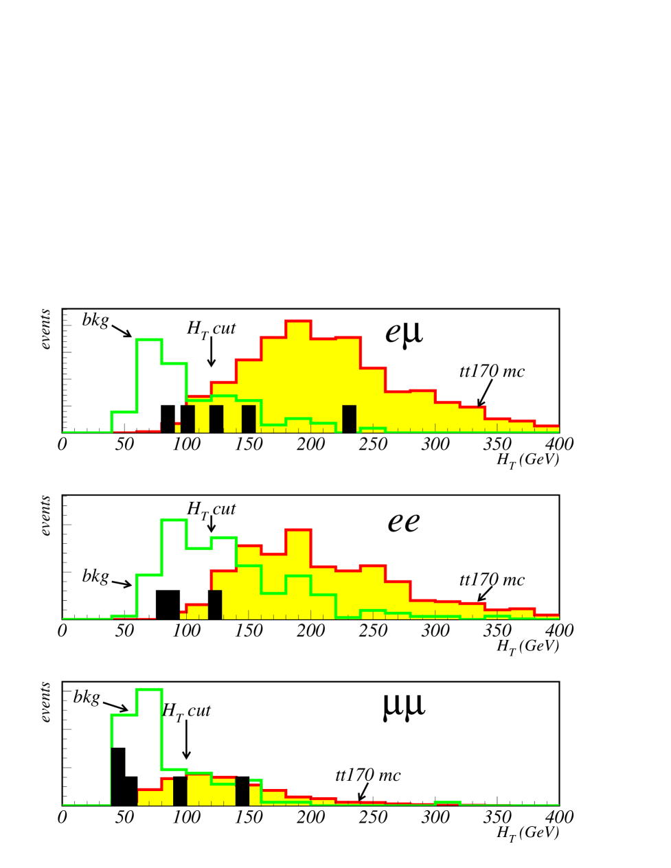
Fig. 26.: $H_{T}$ distributions of dilepton events (for $m_{t}=170~{}\text{GeV}/c^{2}$) in the DØ analyses. The location of observed events is shown by dark histograms.

DØ sought to increase the $t\overline{t}$ acceptance by using the “$e\nu$” channel to recover some events that fail the standard kinematic selection. This channel requires only a single electron, but has very high ${\hbox{$E$\kern-6.00006pt\lower-0.43057pt\hbox{/}}}_{T}$ and jet cuts. It is populated by events from the channels $ee$, $e\mu$, and $e+\text{jets}$, and yields four events that pass the selection criteria listed in Table 9. We note that the significance of these data is comparable to that of the dilepton data; therefore, the $e\nu$ channel makes a useful contribution to the cross section measurement.

Table 9.: Kinematic event selection criteria for various $t\overline{t}$ decay channels applied in the cross section analysis by DØ. All energies are in GeV, $\eta$ is the pseudorapidity, $H_{T}=\sum E_{T}^{\text{jet}}$ with $E_{T}^{\text{jet}}>15~{}\text{GeV}$, and $H_{T}^{e}=H_{T}+E_{T}^{e}$.

	Dilepton	$\ell+\text{jets}$	$\ell+\text{jets}/\mu$	$e\nu$
Lepton $p_{T}$	$>15$	$>20$	$>20$	$>20$
	$>20$ ($ee$)
Electron $|\eta|$	$<2.5$	$<2.0$	$<2.0$	$<1.1$
Muon $|\eta|$	$<1.7$	$<1.7$	$<1.7$	—
${\hbox{$E$\kern-6.00006pt\lower-0.43057pt\hbox{/}}}_{T}$	$>20$ ($e\mu$)	$>25$ ($e$)	$>20$	$>50$
	$>25$ ($ee$)	$>20$ ($\mu$)
Jet $E_{T}$	$>20$	$>15$	$>20$	$>30$
Jet $|\eta|$	$<2.5$	$<2.0$	$<2.0$	$<2.0$
Number of jets	$\geq 2$	$\geq 4$	$\geq 3$	$\geq 2$
$H_{T}^{e}$	$>120$ ($ee$,$e\mu$)	—	—	—
$H_{T}$	$>100$ ($\mu\mu$)	$>180$	$>110$	—
${\cal{A}}$	—	$>0.065$	$>0.040$	—
$E_{T}^{L}$	—	$>60$	—	—
$|\eta^{W}|$	—	$<2.0$	—	—
Tag muon	—	veto	$p_{T}$ $>4$	—
			$\Delta{\cal R}(\mu,\text{jet})$ $<0.5$
$M_{T}^{e\nu}$	—	—	—	$>115$

The main backgrounds in the dilepton channels are from $Z$ boson, Drell-Yan, and diboson processes. In the $ee$ channel, the large background from $Z\rightarrow ee$ is reduced by tightening the ${\hbox{$E$\kern-6.00006pt\lower-0.43057pt\hbox{/}}}_{T}$ cut from $25~{}\text{GeV}$ to $40~{}\text{GeV}$ if the dielectron mass lies within $12~{}\text{GeV}$ of the mass of the $Z$ boson. For the $\mu\mu$ channel, the $Z+\text{jets}$ background is also dominant. Because the $\mu\mu$ and $ee$ channels have identical kinematics one could, in principle, apply the same cuts in both cases. However, DØ does not measure the momenta of muons as well as those of electrons. Consequently, the missing transverse energy is more susceptible to mismeasurements of muon momenta, and is therefore less useful as a variable to discriminate signal from background. Instead, events are fit to the $Z(\rightarrow\mu\mu)+\text{jets}$ hypothesis; events with acceptable fits ($\text{Prob}(\chi^{2})>1$%) are rejected. The $e\mu$ channel, by contrast, is particularly clean: with the selection criteria given in Table 9, DØ obtains a signal to background ratio of $10:1$. Half the background comes from $Z\rightarrow\tau\tau$ events.

The $W(\rightarrow e\nu)+\text{jets}$ background, the main background in the $e\nu$ channel, is very effectively reduced by the application of a large transverse mass requirement: $M_{T}^{e\nu}>115~{}\text{GeV}$, where $M_{T}^{e\nu}\equiv\sqrt{2|p_{T}^{e}||p_{T}^{\nu}|-2p_{T}^{e}\cdot p_{T}^{\nu}}$. The size of the background is estimated from data: one scales down the number of $W+\geq 2~{}\text{jets}$ events by the efficiency of the transverse mass cut, the latter determined from a simulation of $W+\geq 2~{}\text{jets}$ events using the vecbos program.

The systematic uncertainties mainly arise from the uncertain knowledge of the jet energy scale and Monte Carlo modeling, and are estimated to be between 10 and 15%. The $\mu\mu$ channel has an additional uncertainty of $10\%$, due to the $Z\rightarrow\mu\mu$ kinematic fit. From these channels, DØ measures $\sigma_{t\overline{t}}(m_{t}=172.1~{}\text{GeV}/c^{2})=6.4\pm 3.3~{}\text{pb}$.

5.3.2 Lepton+Jets Channels

The lepton + jets channels include the $e+\text{jets}$ and $\mu+\text{jets}$ subchannels. These events are divided into two disjoint subsamples: untagged ($\ell+\text{jets}$) and (SLT) tagged ($\ell+\text{jets}/\mu$). The major background for both of these subsamples is from $W+\text{jets}$ events. There is also a smaller component from QCD multijet events, in which one jet fakes a lepton signature.

The cuts imposed for the untagged $\ell+\text{jets}$ channel are summarized in Table 9, the basic requirements being a high-$p_{T}$ central lepton, large ${\hbox{$E$\kern-6.00006pt\lower-0.43057pt\hbox{/}}}_{T}$, four jets, and no $b$-tag. For the first half of Run 1b, the muon acceptance was restricted to $|\eta|<1.0$ because of radiation damage in the forward muon chambers. For Run 1a and the second half of Run 1b (after the damage was repaired), the acceptance extended out to $|\eta|<1.7$. The variable $\eta^{W}$ shown in the table is the pseudorapidity of the $W$-vector formed by combining the lepton and the ${\hbox{$E$\kern-6.00006pt\lower-0.43057pt\hbox{/}}}_{T}$. The longitudinal component is found by constraining the lepton-neutrino pair to the $W$ boson mass. A cut $|\eta^{W}|<2.0$ is imposed because DØ observes that vecbos, which is used to model the kinematics of the $W+\text{jets}$ background, does not agree well with data in the forward region.[d0ljtopmassprd] The cut has very little effect on the top quark signal, however. The variable $E_{T}^{L}$ is defined as the scalar sum of the lepton momentum and the ${\hbox{$E$\kern-6.00006pt\lower-0.43057pt\hbox{/}}}_{T}$. It is useful mainly for rejecting QCD multijets background; again, this cut does not have much effect on the $t\overline{t}$ signal.

DØ also applies cuts in the $({\cal{A}},H_{T})$ plane. The cut values are chosen through an exhaustive search of possible cuts in order to optimize the expected precision of the cross section measurement. The search method used by DØ, called the random grid search,[rgs] was a key development as it provides a highly efficient way to search $n$-dimensional parameter spaces. It differs from a conventional grid search in that the grid of cuts is determined by the expected distribution of the signal; hence the term “random” grid. The results of the search, along with the optimal cuts, are shown in Fig. 27. The distribution of events in the $({\cal{A}},H_{T})$ plane is shown in Fig. 28. Nineteen events survive all the cuts.

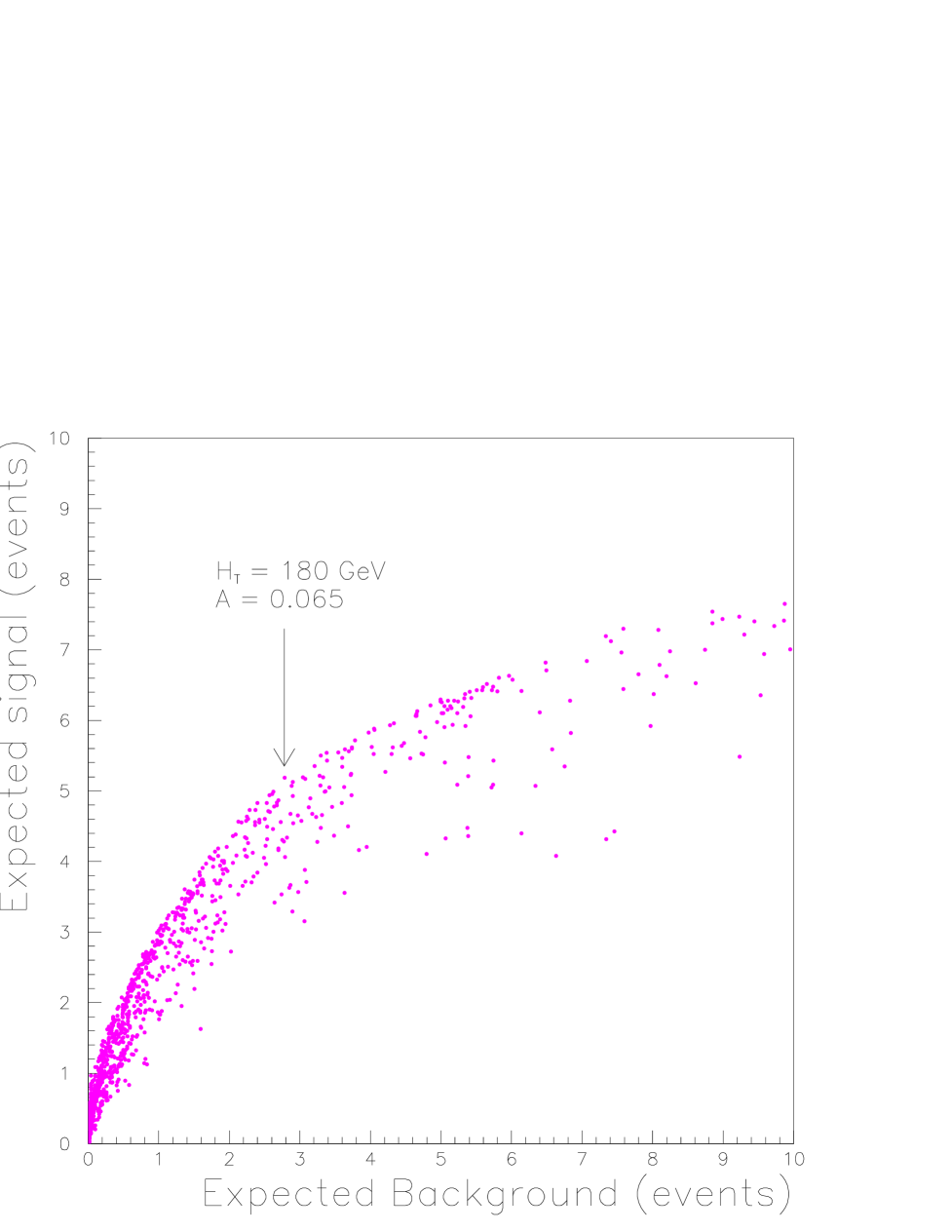
Fig. 27.: Expected signal (for $m_{t}=180~{}\text{GeV}/c^{2}$, $e+\text{jets}$ channel) versus background yields in $77~{}\text{pb}^{-1}$ for various cuts on ${\cal{A}}$ and $H_{T}$. The arrow identifies the optimal cut found by the random grid search method.

Fig. 28.: Distributions the in $({\cal{A}},H_{T})$ plane for data (top left), $t\overline{t}$ MC (top right), multijet background (bottom left), and $W+\text{jets}$ vecbos MC (bottom right). From Ref. [d0xsecprl97].

The QCD multijets background is estimated from data by first measuring the probability for a jet to fake a lepton signature, and then directly applying these probabilities to the QCD multijets data. The dominant $W+\text{jets}$ background is estimated using the technique of “Berends scaling.” This is based on the observation that the number of $W+\text{jets}$ events falls off exponentially with the number of jets.[d0topprd, vecbos] Thus, after subtracting the contribution from QCD multijets background, DØ extrapolates from the number of $\ell+\text{jets}$ events observed at low multiplicities to estimate the number of $W+\text{jets}$ events with at least four jets. The efficiency for these $W+\text{jets}$ events to pass the $({\cal{A}},H_{T})$ requirement is estimated using vecbos. By this procedure, DØ estimates the background to be $8.7\pm 1.7$ events. About $15\%$ of this background is due to QCD multijet events; the rest is from $W+\text{jets}$.

DØ finds that the dominant systematic uncertainty of 15% is due to the differences in the $({\cal{A}},H_{T})$ distributions between data and the corresponding simulations of $W+2~{}\text{jet}$ and $W+3~{}\text{jet}$ events. The uncertainty due to possible departures from the Berends scaling law is found to be 10%. The jet energy scale uncertainty, however, is only 5%. With 19 candidate events and a background of $8.7\pm 1.7$ events, the measured cross section for the $\ell+\text{jets}$ channel is $\sigma_{t\overline{t}}(m_{t}=172.1~{}\text{GeV}/c^{2})=4.1\pm 2.1~{}\text{pb}$.

The cuts for the tagged channels $\ell+\text{jets}/\mu$ are summarized in Table 9. Note that for these channels, only three jets are required, as opposed to four for the untagged channels. The $({\cal{A}},H_{T})$ cuts are also looser. This is to compensate for the loss of acceptance caused by requiring events to be tagged. To reject QCD multijets background, DØ makes the cuts:[d0topprd]

• $e+\text{jets}/\mu$ channel: $\mbox{${\hbox{$E$\kern-6.00006pt\lower-0.43057pt\hbox{/}}}_{T}$}>35~{}\text{GeV}$ if $\Delta\phi(\mbox{${\hbox{$E$\kern-6.00006pt\lower-0.43057pt\hbox{/}}}_{T}$},\mu)<25^{\circ}$.

• $\mu+\text{jets}/\mu$ channel: $\Delta\phi(\mbox{${\hbox{$E$\kern-6.00006pt\lower-0.43057pt\hbox{/}}}_{T}$},\mu)<170^{\circ}$ and $|\Delta\phi(\mbox{${\hbox{$E$\kern-6.00006pt\lower-0.43057pt\hbox{/}}}_{T}$},\mu)-90^{\circ}|/90^{\circ}<\mbox{${\hbox{$E$\kern-6.00006pt\lower-0.43057pt\hbox{/}}}_{T}$}/(45~{}\text{GeV})$.

In addition, in the $\mu+\text{jets}/\mu$ channel, DØ rejects $Z\rightarrow\mu\mu$ background using a kinematic fit to the $Z$ boson decay hypothesis. With these cuts, eleven candidates survive.

The $W+\text{jets}$ background is computed by starting with the assumption that the heavy flavor content of $W+\text{jets}$ events is the same as that in multijet events. Therefore, from the tag probability per jet $p_{j}$, as determined from a multijet sample (and parameterized in terms of $E_{T}$ and $\eta$), DØ determines the tagged $W+\text{jets}$ background by weighting a sample of background-dominated untagged events by the per-event tag probability $\sum_{j}p_{j}$, where the sum runs over all jets.

Figure 29 compares the observed numbers of events for different jet multiplicities to the background prediction. The agreement for the one and two jet samples is good, while for three or more jets there is a clear excess of events. The estimated background in the $\geq 3~{}\text{jet}$ signal region is $2.4\pm 0.5$ events, including a $10\%$ systematic uncertainty due to the tagging procedure. The measured cross section for these channels is $\sigma_{t\overline{t}}(m_{t}=172.1~{}\text{GeV}/c^{2})=8.3\pm 3.5~{}\text{pb}$.

Fig. 29.: Jet multiplicity of $b$-tagged lepton+jets events before ${\cal{A}}$ and $H_{T}$ cuts. Square points represent data and the circles the expected background. From Ref. [d0xsecprl97].

5.3.3 All-Jets Channel

The all-jets channel, as we noted earlier, suffers from a huge QCD background. It is a channel for which $b$-tagging is particularly effective and DØ, like CDF, takes advantage of this. However, since DØ cannot tag $b$-jets nearly as efficiently as CDF, extensive use is made of multivariate methods, in order to exploit other, more subtle, differences between the signal and the background. The resulting analysis[amos98, klima98, d0alljetsprd] is rather complex; therefore, we focus here on only the key ideas.

The measurement of the $t\overline{t}$ production cross section in the all jets channel is based on an integrated luminosity of $110~{}\text{pb}^{-1}$. The trigger used is sensitive to events with many jets and large $H_{T}$. The initial selection cuts are:

• No isolated leptons. This ensures that there is no overlap with the other channels.

• $H_{T}>115~{}\text{GeV}$ (using jets with $R=0.5$, $E_{T}>15~{}\text{GeV}$, and $|\eta|<2.5$).

• At least six $R=0.3$ cone jets and no more than eight $R=0.5$ cone jets (with $E_{T}>10~{}\text{GeV}$ and $|\eta|<2.5$). Both of these requirements improve the signal/background ratio: the lower bound rejects only $14\%$ of the signal while removing $36\%$ of the background, and the upper bound loses $5\%$ of the signal but $13\%$ of the background.

Additional cuts are applied to remove events with noise from the Main Ring. After these cuts, about 280,000 events remain. At this stage, the signal to background ratio is about $1:1000$. Requiring an SLT $b$-tag increases the signal/background by about an order of magnitude, leaving 6000 events.

To make further progress, DØ performs a multivariate analysis using thirteen variables, described briefly in Table 10. The principal ones are $H_{T}$, $H_{T3}\equiv H_{T}-E_{T}^{\text{jet}1}-E_{T}^{\text{jet}2}$, the average jet count $N_{\text{jets}}^{A}$, the aplanarity ${\cal A}$, the centrality $C\equiv H_{T}/\sum_{\text{jets}}E^{\text{jet}}$, and the transverse momentum of the muon $p_{T}^{\mu}$. A particularly powerful (and unusual) variable is the average jet count, defined by

$$N_{\text{jets}}^{A}={\int_{15~{}\text{GeV}}^{55~{}\text{GeV}}E_{T}N(>E_{T})\;dE_{T}\Bigg{/}\int_{15~{}\text{GeV}}^{55~{}\text{GeV}}E_{T}\;dE_{T}},$$ (19)

where $N(>E_{T})$ is the number of jets with transverse energy greater than $E_{T}$. This variable, inspired by the work of Tkachov,[tkachov95] is interesting in that it assigns a nonintegral “number of jets” to an event.

Table 10.: List of variables used by DØ in its all-jets cross section measurement. The $Q_{i}$ are the eigenvalues (in increasing size) of the normalized momentum tensor $M_{ab}=\sum_{j}P_{ja}P_{jb}/\sum_{j}|P_{j}|^{2}$ of the jets in the event; $a,b$ run over the $x,y,z$ components of the jet momenta $P_{j}$.

Variable	Description
$H_{T}$	Total jet transverse energy
$\sqrt{\hat{s}}$	Total $t\overline{t}$ center of mass energy
$H_{T3}$	Transverse energy of the non-leading jets
$N_{\text{jets}}^{A}$	Average jet count (see text for details)
${\cal{A}}$	Aplanarity ($\frac{3}{2}Q_{1}$)
${\cal S}$	Sphericity ($\frac{3}{2}(Q_{1}+Q_{2})$)
${\cal C}$	Centrality ($H_{T}/\sum_{\text{jets}}E^{\text{jet}}$)
$E_{T}^{\text{jet}1}/H_{T}$	Transverse energy fraction of leading jet
$\sqrt{E_{T}^{\text{jet}5}E_{T}^{\text{jet}6}}$	Geometric mean of $E_{T}$ of the fifth and sixth jets
$\left\langle\eta^{2}\right\rangle$	Mean square rapidity of all jets
$p_{T}^{\mu}$	Transverse momentum of the tag muon
$\cal F$	Fisher discriminant: A measure of the difference
	in jet widths between signal and background
$\cal M$	Mass likelihood: A measure of the degree to which
	jet invariant masses satisfy the constraints that there
	be two $W$ bosons and that the two top quarks have
	equal mass.

These thirteen variables are combined using feed-forward neural networks into a single discriminant $NN_{2}$, the value of which lies between zero and unity. This is done in three steps:

• $NN_{0}$ — a network is trained with the first seven variables listed in Table 10, using all events; this network is used to select better event samples for training the subsequent networks.

• $NN_{1}$ — a network is trained with the first ten variables of Table 10, having twenty hidden nodes and one output node, using events which satisfy the cut $NN_{0}>0.3$.

• $NN_{2}$ — a final network is trained, using events with $NN_{0}>0.3$, with four input nodes, eight hidden nodes and one output node; the inputs are the output of $NN_{1}$ plus the remaining three variables.

Since the data are predominantly background, DØ uses untagged events as the background sample in the training, and tagged herwig $t\overline{t}$ Monte Carlo events (with $m_{t}=180~{}\text{GeV}/c^{2}$) for the signal. There is, however, a complication. Untagged events, by definition, do not have muons; but the latter are nonetheless needed to train $NN_{2}$! The solution adopted is to generate Monte Carlo muons according to the measured muon $p_{T}$ spectrum and to add them to the untagged sample, thereby transforming the background sample into a tagged sample. One might worry that this procedure would fail because of correlations between the muon $p_{T}$ and the remaining variables. If correlations exist, the incoherent addition of Monte Carlo muons to untagged events would not be expected to reproduce the characteristics of tagged events.

However, the procedure works. As shown in Fig. 30, the muon $p_{T}$ is uncorrelated with the $E_{T}$ of the tagged jet, provided that the tagged jet is not corrected for the presence of the muon. This absence of correlation between muon $p_{T}$ and jet $E_{T}$ precludes the existence of correlation between the muon $p_{T}$ and the rest of the event.

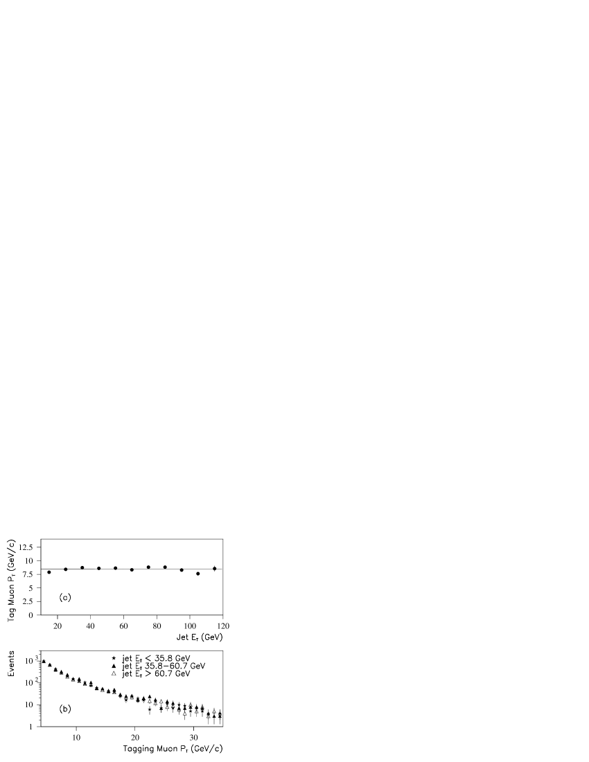
Fig. 30.: (a) The mean muon $p_{T}$ versus jet $E_{T}$, as observed by DØ in their all-jets cross section analysis. We see that the muon $p_{T}$ is independent of the jet $E_{T}$. (b) The observed muon $p_{T}$ distribution for three jet $E_{T}$ ranges (normalized to the same number of events). From Ref. [d0alljetsprd].

The background to the tagged data is estimated by weighting the untagged data (with the Monte Carlo muons) by the tag probability per event. Figure 31 illustrates how well the weighting procedure works. The figure shows an absolute comparison of the tagged events to the predictions for the thirteen variables. For all variables, the agreement is seen to be good.

Fig. 31.: A comparison of DØ’s absolute predictions (histograms) for the distributions of the thirteen variables used in the all-jets cross section measurement: (a) $H_{T}$ (GeV), (b) $\sqrt{\hat{s}}$ (GeV), (c) $E_{T}^{\text{jet}1}/H_{T}$, (d) $H_{T3}$ (GeV), (e) $N_{\text{jets}}^{A}$, (f) $\sqrt{E_{T}^{\text{jet}5}E_{T}^{\text{jet}6}}$ (GeV), (g) ${\cal{A}}$, (h) ${\cal S}$, (i) ${\cal C}$, (j) $\left\langle\eta^{2}\right\rangle$, (k) $p_{T}^{\mu}$, (l) $\cal F$, and (m) $\cal M$. The points represent the observed data in a sample of 3853 tagged events. From Ref. [d0alljetsprd].

To extract the cross section, DØ fits the observed $NN_{2}$ distribution for tagged events to the expectations for signal and background. The fit is performed for the 2207 tagged events that pass the cut $NN_{2}>0.02$. The results of the fit (for $m_{t}=180~{}\text{GeV}/c^{2}$) are shown in Fig. 32. This gives a cross section for $m_{t}=180~{}\text{GeV}/c^{2}$ of $6.3\pm 2.5\ \text{(stat)}~{}\text{pb}$. The major systematic uncertainties in this measurement are in the background tag probability (7%), the $t\overline{t}$ tag probability (7%), the modeling of the muon $p_{T}$ spectrum, and the jet energy scale (9%). After interpolating to the measured top quark mass, the final result is $\sigma_{t\overline{t}}(m_{t}=172.1~{}\text{GeV}/c^{2})=7.1\pm 2.8~{}\text{(stat)}\pm 1.5~{}\text{(syst)}~{}\text{pb}$.

Fig. 32.: The distribution of the final neural network output ($NN_{2}$) in the DØ all-jets cross section analysis showing the results of a fit of the observed tagged distribution to the predictions for signal and background, with $m_{t}=180~{}\text{GeV}/c^{2}$. Only statistical errors are shown, and events with $NN_{2}<0.02$ are not plotted. The fit has a $\chi^{2}$ per degree of freedom of 16.9/17. From Ref. [d0alljetsprd].

As a cross check, DØ also estimates the cross section using the usual counting method. Here, a cut $NN_{2}>0.85$ is imposed. This yields 41 observed events, with an estimated background of $24\pm 2.4$ events. The signal efficiency at $m_{t}=180~{}\text{GeV}/c^{2}$ is $0.022\pm 0.0037$, yielding a cross section of $6.5\pm 2.6~{}\text{(stat)}\pm 1.4~{}\text{(syst)}~{}\text{pb}$, in good agreement with that found by the fit. If the cut value is reoptimized to maximize the expected significance (using Monte Carlo), the result is $NN_{2}>0.94$, yielding 18 observed events and an estimated background of $6.9\pm 0.9$ events. The chance of this background fluctuating to give at least the observed signal is $6\times 10^{-4}$, or a $3.2\sigma$ deviation for a Gaussian.

Table 11.: Summary of DØ cross section measurements, for $m_{t}=172.1~{}\text{GeV}/c^{2}$.

Channel	$\epsilon\times\text{BR}(\%)$	Data	Background	$\sigma_{t\overline{t}}$ (pb)
$\ell\ell$ (with $e\nu$)	$0.91\pm 0.17$	9	$2.6\pm 0.6$	$6.4\pm 3.3$
$\ell+\text{jets}$ (untagged)	$2.28\pm 0.46$	19	$8.7\pm 1.7$	$4.1\pm 2.1$
$\ell+\text{jets}/\mu$	$0.96\pm 0.15$	11	$2.4\pm 0.5$	$8.3\pm 3.5$
$\ell\ell$ and $\ell+\text{jets}$	$4.14\pm 0.69$	39	$13.7\pm 2.2$	$5.6\pm 1.8$
All-jets ($NN_{0}>0.85$, $m_{t}=180~{}\text{GeV}/c^{2}$)	$2.2\pm 0.4$	41	$24\pm 2.4$	$6.5\pm 3.0$
All-jets (from fit)				$7.1\pm 3.2$
Total				$5.9\pm 1.7$

5.4 Summary of Cross Section Measurements

The results of the CDF and DØ cross section analyses are summarized in Tables 8 and 11, respectively, and graphically in Fig. 33.

Excluding the all-jets channel, DØ observes a total of 39 events with a background of $13.7\pm 2.2$ events. For a top quark mass of $172.1~{}\text{GeV}/c^{2}$ this gives a measured cross section of $5.6\pm 1.8~{}\text{pb}$. If the measurement from the all-jets channel is included, the result changes to $5.9\pm 1.7~{}\text{pb}$. The measurement from CDF, which includes all channels except the $\tau$-dilepton channels, is $\sigma_{t\overline{t}}=7.6^{+1.8}_{-1.5}~{}\text{pb}$ for a top quark mass of $175~{}\text{GeV}/c^{2}$. Both results are presented graphically in Fig. 34, which compares the measurements to several predictions. Although the cross sections obtained by CDF are typically higher than those from DØ, both sets of results are consistent with each other and with predicted values. The results are also consistent with the expected branching ratios.

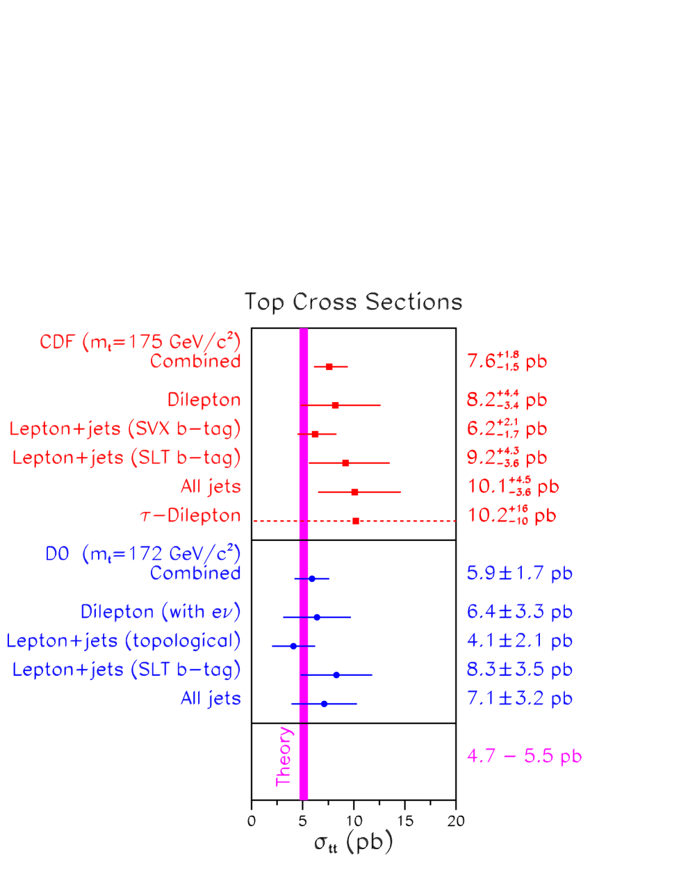
Fig. 33.: The $t\overline{t}$ production cross section measured in the channels studied by CDF and DØ. Also shown is the range of predictions from various theoretical calculations.

Fig. 34.: The $t\overline{t}$ production cross sections as measured by CDF and DØ. Also shown are various theoretical calculations.[laenen94, berger95, bonciani98]

6 Measurement of the Top Quark Mass

Early direct measurements of the top quark mass were published in the papers announcing the observation of the top quark in 1995.[cdfdiscovery, d0discovery, wimpenny96] Since that discovery, the two collaborations have mounted prodigious efforts to measure the top quark mass as precisely as possible. It is to these results that we now turn. After sketching the analysis strategies used by the two collaborations, we describe in greater detail interesting aspects of the analyses of CDF and DØ. We end with a summary of the results.

6.1 General Strategy

Both collaborations use two different strategies to measure the mass of the top quark. The first involves kinematically fitting the events to a $t\overline{t}$ hypothesis and then extracting from the fits an estimate of the mass of the top quark. The second strategy is based on constructing mass-dependent variables that do not require a kinematic fit.

In the first strategy, one tries to identify the observed objects (jets, leptons, and missing transverse energy) with those at the partonic level. To the degree that such an identification is possible, one can perform a kinematic fit of the observed event to the $t\overline{t}$ decay hypothesis. When the mass of the top quark is extracted from such a fit, it is commonly called the fitted mass. Because the $t\overline{t}$ decay hypothesis does not always hold true, this is not the same as the true top quark mass; nevertheless, it is a well-defined observable, the mean of which depends on the mass of the top quark. This defines one class of mass-dependent observables or variables.

The principal advantage of a kinematic fit is that, generally, the resulting variables have the greatest sensitivity to the mass of the top quark. But such fits are not always possible; this is so, for example, if there are fewer observed jets than partons.

The alternative strategy eschews the complexities of a kinematic fit, and instead uses one or more kinematic quantities that are known to be mass-dependent. An example of such a variable is $H_{T}=\sum E_{T}^{\text{jet}}$, the scalar sum of the jet transverse energies. The disadvantage of this approach is that variables such as $H_{T}$ tend to have much broader distributions than those of the fitted mass. On the other hand, this approach is simple and direct (compared with kinematic fitting), and it can be used for all events. Moreover, it may ultimately be the more satisfactory strategy for the following reason. As the accuracy of the mass measurements improve, we shall reach a point when the quantum nature of partonic decay can no longer be neglected and our classical one-to-one identification of a jet with a parton will break down.[giele97] When this point is reached, it may be necessary to use observables that do not require forcing a one-to-one map back to the partonic level. Ultimately, the limitation will be the sensitivity of the mass to the QCD modeling of the final state.

Each strategy furnishes a mass-dependent variable $x$ per event, the distribution of which, $f(x)$, depends upon the mass of the top quark $m_{t}$ if the event is a top quark event. The functions $f_{s}(x|m_{t})$ and $f_{b}(x)$ pertaining to the signal and background, respectively, are calculated using detailed Monte Carlo simulations of the signal and background reactions. The functions $f_{s}(x|m_{t})$ and $f_{b}(x)$ are sometimes referred to as templates. Given a set of templates and a set of measurements $(x_{1},\cdots,x_{n})$, there are a variety of standard methods available, most commonly maximum likelihood,[MaxLikelihood] to extract a single estimate of the parameter of interest, here the mass $m_{t}$.

Much of the effort in these analyses is devoted to constructing reliable templates. This is a delicate matter because of the necessary reliance on complicated Monte Carlo simulations to compute them. The key issue, of course, is to establish that the templates, so obtained, agree with the data. For the background, this is less of an issue because the data, being largely background, afford a direct check of the correctness of those templates in regions of parameter space that are relatively free of signal. However, for the signal, the verification of the templates is, necessarily, more problematic because the signal events are generally less numerous. It is therefore notable that in spite of these difficulties, both collaborations have been able to produce very precise and consistent results.

At a fundamental level, there is really no difference between the two strategies we have outlined: the result of the kinematic fit is a mass-dependent kinematic quantity, albeit a particularly complicated one. Nevertheless, the practical details of carrying out the analyses are sufficiently different that the distinction is worth making.

In the following sections we describe how these strategies have been realized by each collaboration. We begin with the analyses of CDF, followed by those of DØ.

6.2 CDF Analyses

The CDF collaboration has measured the top quark mass in all of the dilepton, lepton+jets, and all jets channels, using their full Run 1 data sample.

6.2.1 Dilepton Channels

In this analysis,[cdfdilep98] CDF considers the channels $e\mu$, $\mu\mu$, and $ee$, in which both $W$ bosons decay leptonically. The mass analysis starts with the same data sample and cuts as used in the dilepton cross section analysis (see Sec. 5.2 and Table 5). To improve the signal/background ratio beyond the level used for the cross section analysis, CDF imposes the cut $H_{T}^{\text{all}}>170~{}\text{GeV}$, where $H_{T}^{\text{all}}=p_{T}^{\ell 1}+p_{T}^{\ell 2}+E_{T}^{\text{jet}1}+E_{T}^{\text{jet}2}+\mbox{${\hbox{$E$\kern-6.00006pt\lower-0.43057pt\hbox{/}}}_{T}$}$ is the sum of the transverse momenta of the two leptons, the transverse energies of the two highest-$E_{T}$ jets, and the missing transverse energy. The power of such variables to discriminate signal from background was recognized early on,[baer89] and was first applied to good effect by DØ.[d0topprd, d0xsecprl95] With this final cut, the sample is reduced to eight events with an estimated background of $1.3\pm 0.3$ events. The CDF collaboration then estimates the top quark mass using two different methods.

Both methods are a realization of the second strategy, being based on relatively simple mass-dependent kinematic variables. For the first method, CDF uses the observation that the energies of the $b$-quarks are sensitive to the mass of the top quark, $m_{t}$. Indeed, it is found that the mean energy of the two highest $E_{T}$ jets depends linearly on $m_{t}$, with a slope of about 0.5. From Monte Carlo simulations, CDF obtains a set of templates $f(E|m_{t})$ describing the observed jet energy distribution, one for each top quark mass considered in the range 100 to $240~{}\text{GeV}/c^{2}$. Templates are also constructed for the backgrounds. CDF then performs a maximum likelihood fit of the observed distribution of jet energies to a mixture of $t\overline{t}$ and background events, with the background count constrained to $1.3\pm 0.3$ events. For each assumed top quark mass $m$, $-\ln\left({\cal L}(m)\right)$, where ${\cal L}(m)$ is the value of the likelihood at that mass, is calculated. By fitting a third order polynomial to the negative logarithms, and using the position of its minimum as an estimate of the mass, CDF obtains the mass estimate $159\pm 23~{}\text{(stat)}\pm 11~{}\text{(syst)}~{}\text{GeV}/c^{2}$. Following standard practice, CDF defines the statistical error by applying the “0.5-rule”: the error is the mass difference, relative to the value at the minimum ($159~{}\text{GeV}/c^{2}$), that increases $-\ln({\cal L})$ by 0.5. Figure 35a shows the jet energy distribution and the resulting log-likelihood function.

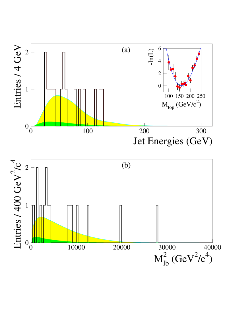
Fig. 35.: (a) The energy distribution of the two highest $E_{T}$ jets for the CDF dilepton events (histogram, two entries per event). The lightly shaded curve is the prediction for $t\overline{t}$ signal ($m_{t}=160~{}\text{GeV}/c^{2}$) plus background, and the heavily shaded curve is the prediction for background alone. The inset shows the $-\ln({\cal L})$ fit as a function of $m_{t}$. (b) The distribution of ${M^{2}_{{\ell b}_{\min}}}$ (histogram, two entries per event). The shaded curves are as in (a). From Ref. [cdfdilep98].

The second method exploits the relationship between $m_{t}$ and the invariant mass ${M_{\ell b}}$ of the lepton and the associated $b$-quark. Since the top quark decays to a $b$-quark and a $W$ boson, we can write $m_{t}^{2}=m_{b}^{2}+M_{W}^{2}+2E_{b}M_{W}$, where $E_{b}$ is the energy of the $b$-quark in the rest frame of the $W$ boson. The $b$-quark’s energy $E_{b}$, which is constant in the $W$ boson rest frame, can be calculated from the mean invariant mass $\left\langle{M_{\ell b}}\right\rangle$ and opening angle $\left\langle\cos\theta_{{\ell}b}\right\rangle$ between the $b$-quark and the lepton: $\left\langle{M^{2}_{\ell b}}\right\rangle=E_{b}M_{W}(1-\left\langle\cos\theta_{{\ell}b}\right\rangle)$. To lowest order in the Standard Model, $\left\langle\cos\theta_{{\ell}b}\right\rangle=M_{W}^{2}/(m_{t}^{2}+2M_{W}^{2})$, which leads to $m_{t}^{2}=\left\langle{M^{2}_{\ell b}}\right\rangle+\sqrt{M_{W}^{4}+4M_{W}^{2}\left\langle{M^{2}_{\ell b}}\right\rangle+\left\langle{M^{2}_{\ell b}}\right\rangle^{2}}$. Given this relationship, a measurement of $\left\langle{M^{2}_{\ell b}}\right\rangle$ is tantamount to a direct measurement of $m_{t}$. (For an interesting variation on this theme, see Ref. [prosper95].)

Unfortunately, there is a difficulty: a priori, we do not know which jet should be paired with which lepton; whether $(\ell^{+}j_{1},\ell^{-}j_{2})$ is the correct $(\ell^{+}b,\ell^{-}\overline{b})$ assignment or $(\ell^{+}j_{2},\ell^{-}j_{1})$. In addition, since ${M_{\ell b}}$ is defined by a quadratic equation, there are two solutions to be considered for each jet configuration. CDF resolves the first of these difficulties by selecting the jet configuration with the smaller sum of invariant masses. This selection is correct 55% to 75% of the time, depending upon the top quark mass. The values of ${M_{\ell b}}$ selected in this manner are denoted ${M_{{\ell b}_{\min}}}$. The second difficulty is dealt with by retaining both solutions, and plotting each event twice. Figure 35b shows the resulting ${M_{{\ell b}_{\min}}}$ distribution for the eight events in the sample, along with the signal and background predictions. Of course, owing to selection biases and jet energy mismeasurements, $\left\langle{M_{{\ell b}_{\min}}}\right\rangle$ is not the same as $\left\langle{M_{\ell b}}\right\rangle$; however, from Monte Carlo studies, CDF finds that the two quantities are linearly related. The result from this method is $m_{t}=163\pm 20~{}\text{(stat)}\pm 9~{}\text{(syst)}~{}\text{GeV}/c^{2}$. Combining this with the previous result, taking into account their mutual correlation, gives $m_{t}=161\pm 17~{}\text{(stat)}\pm 10~{}\text{(syst)}~{}\text{GeV}/c^{2}$.

For both methods, the major sources of systematic uncertainties are the knowledge of the jet energy scale and the shape of the background distributions.

At a recent conference in Vancouver (ICHEP98), CDF presented an updated dilepton channel mass measurement,[roser] using a method similar to the DØ $\nu$WT method (see Sec. 6.3.1). The result of this analysis was $m_{t}=167.4\pm 10.3~{}\text{(stat)}\pm 4.8~{}\text{(syst)}~{}\text{GeV}/c^{2}$. (The details of this analysis were not available in time for inclusion in this review.)

6.2.2 Lepton+Jets Channels

These channels provide CDF with its most precise measurement of the top quark mass.[cdftopmass98] This is due to both the relatively large branching ratios for these channels ($\approx 30\%$) and the large signal/background ratio that can be achieved through $b$-tagging (see Sec. 3.3.6). The event selection used is similar to that used for the cross section analysis (see Table 5), except that four jets are required, and events without a $b$-tag are accepted. But in order to increase the efficiency for the four jet requirement, the cuts on the fourth jet are loosened to $E_{T}>8~{}\text{GeV}$ and $|\eta|<2.4$, provided that one of the four leading jets is $b$-tagged with either the SLT or the SVX algorithm. (For untagged events, all four jets must satisfy $E_{T}>15~{}\text{GeV}$ and $|\eta|<2.0$.) This selection yields a sample of 83 events.

This analysis follows the strategy of kinematic fitting. The observed event is fit to the hypothesis $p\overline{p}\rightarrow t\overline{t}+X\rightarrow(\ell\nu b)(bq\overline{q})+X$, with the four leading jets assumed to map onto the four quarks. The measured variables are the three-momenta of the lepton and the four leading jets, plus the vector sum of all remaining transverse energy (excluding the lepton and the leading jets). This latter vector gives the transverse momentum of the recoiling system $X$. The momentum of the neutrino is not measured, yielding three unknowns. The neutrino and lepton are assumed to be massless, $b$-quarks are assigned a mass of $5~{}\text{GeV}/c^{2}$, and light quarks are assigned a mass of $0.5~{}\text{GeV}/c^{2}$. Five constraints can then be imposed:

• The transverse momentum components of the $t\overline{t}$ + $X$ system are zero.

• The invariant mass of the lepton and neutrino equals $M_{W}$.

• The invariant mass of the $q$ and the $\overline{q}$ equals $M_{W}$.

• The mass of the $t$ equals that of the $\overline{t}$.

Since there are two more constraints than unknowns, this is a 2C fit. It is solved by standard $\chi^{2}$-minimization techniques, resulting, for each event, in a fitted mass $m_{\text{fit}}$ and a $\chi^{2}$ value that is taken as a measure of how well the event satisfies the $t\overline{t}$ hypothesis.

The energy of each jet is adjusted to match as closely as possible the energy of the parton from which the jet is presumed to have originated, starting with corrections of the sort outlined in Sec. 3.3.1. In addition, CDF applies energy corrections derived by directly comparing, in herwig Monte Carlo samples, the energies of partons with the reconstructed jets. These corrections depend on parton flavor; hadronically decaying $b$-quarks, leptonically decaying $b$-quarks, and light quarks are all corrected differently. Clearly, these corrections depend critically on the ability of herwig to model the fragmentation properties of jets. It is therefore pertinent to ask how well these properties are modeled. The answer is, surprisingly well, given the phenomenological nature of the fragmentation model. Detailed studies of the energy flow within jets (see, e.g., Ref.[d0jetshape]) confirm the ability of herwig to model jets accurately.

In the lepton+jets channels, there is considerably more ambiguity in assigning the jets to the partons than is the case for the dilepton channels. There are twelve possible configurations, or assignments of the four leading jets to the four partons. Moreover, one must choose an initial value for the longitudinal component of the neutrino momentum. Using one of the constraints, this quantity can be found to within a two-fold ambiguity. To guard against finding a local minimum, the fit is tried with both starting points, giving a total of up to twenty-four kinematic fits per event. However, jets that are tagged are only assigned to $b$-quarks, thus reducing the number of configurations. The configuration with the smallest $\chi^{2}$ is chosen, but events whose smallest $\chi^{2}$ value exceeds 10 are rejected. This $\chi^{2}$ cut reduces the sample from 83 to 76 events.

The $\chi^{2}$ variable, unfortunately, is not very effective at selecting the correct configuration (see the discussion in Sec. 6.3.2). Consequently, although the standard deviation of the $m_{\text{fit}}$ distribution would be only $\sim 13~{}\text{GeV}/c^{2}$ (for a top quark mass of $175~{}\text{GeV}/c^{2}$) were the selection procedure perfect, CDF finds that, in practice, the standard deviation of the $m_{\text{fit}}$ distribution is approximately double that value.

The CDF collaboration uses a maximum-likelihood method to extract an estimate of the top quark mass from the sample of 76 events. The likelihood function has the form

$${\cal L}={\cal L}_{\text{shape}}(D|m_{t},x_{b},a)\times{\cal L}_{\text{backgr}}(x_{b}|x_{b}^{0})\times{\cal L}_{\text{param}}(a|a^{0}),$$ (20)

where

$${\cal L}_{\text{shape}}(D|m_{t},x_{b},a)=\prod_{i=1}^{N}[(1-x_{b})f_{s}(m_{i}|m_{t},a)+x_{b}f_{b}(m_{i}|a)]$$ (21)

is the joint probability density assigned to the sample of $N$ fitted masses $D\equiv(m_{1},\ldots,m_{N})$; $f_{s}(m_{i}|m_{t},a)$ is the probability density to observe the fitted mass $m_{i}$ given a top quark mass $m_{t}$, assuming that the $i$th event is signal and $f_{b}(m_{i}|a)$ is the probability density to observe $m_{i}$ assuming the event is background; $x_{b}$ is the background fraction; and $a$ denotes the set of parameters that determine the shape of the functions $f_{s}(m_{i}|m_{t},a)$ and $f_{b}(m_{i}|a)$. These functions (templates) are derived from Monte Carlo calculations (based on herwig for top events and vecbos for the $W$+jets background). In previous work,[cdfdiscovery] CDF used a discrete set of templates. However, the collaboration now finds that smaller systematic uncertainties result from deriving from the discrete set a smooth parameterization of $f_{s}(m_{i}|m_{t},a)$, both in $m_{i}$ and in $m_{t}$. (Amusingly, DØ, which earlier used parameterized templates, now finds it better to use a discrete set!)

These functions contain parameters $a$, other than $m_{t}$, that define the shape of the functions. The parameters have estimates $a^{0}$ and uncertainties that are encoded in the likelihood function ${\cal L}_{\text{param}}$. This likelihood function constrains the shape of the templates in ${\cal L}_{\text{shape}}$ to vary within their uncertainties. The shape parameter uncertainties reflect simply the finite statistics of the Monte Carlo event samples that were used to generate the discrete set of templates.

The background fraction $x_{b}$ is constrained within its uncertainty to the independently measured background fraction $x_{b}^{0}$ by the background likelihood function ${\cal L}_{\text{backgr}}(x_{b}|x_{b}^{0})$. One can think of ${\cal L}_{\text{backgr}}$ and ${\cal L}_{\text{param}}$ as prior probabilities with respect to the likelihood function ${\cal L}_{\text{shape}}$. They encode the information $(a^{0},x_{b}^{0})$ that is known about the background fraction and the shape of the templates.

In statistical analysis, it is sometimes advantageous to use stratified sampling;[FredJames] that is, to divide a sample into two or more subsamples. This is especially true when the characteristics vary widely from one subsample to another. In order to make optimal use of all the available information, the event sample is divided into disjoint subsamples. Each subsample is assigned its own likelihood function in accordance with Eq. (20), the product of which is then maximized to obtain the final estimate of the top quark mass and its uncertainty. From Monte Carlo studies, CDF concludes that four subsamples give the optimum partition:

• events with a single SVX tag,

• events with two SVX tags,

• events with an SLT tag but no SVX tag, and

• events with no tag but with all four leading jets satisfying $E_{T}>15~{}\text{GeV}$ and $|\eta|\leq 2$.

The expected background fraction $x_{b}^{0}$ in each subsample is derived from the $W+\geq 3~{}\text{jets}$ background estimate used in the $t\overline{t}$ cross section measurement (see Sec. 5.2). To estimate the background in the subsamples, one needs the efficiencies of the additional cuts, including the fourth jet requirement and the $\chi^{2}$ cut. These efficiencies are determined from Monte Carlo studies. Using the tagging efficiencies from the cross section analysis and the background rates for the subsample, CDF writes the total mean number of events $n$ in each subsample as a function of the mean number of signal and background events $S$ and $B$, respectively, in the combined sample; that is, $n=\epsilon_{s}S+\epsilon_{b}B$, where $\epsilon_{s}$ and $\epsilon_{b}$ are known fractions, derived from the Monte Carlo studies. The parameters $S$ and $B$ are then estimated by maximizing a multinomial likelihood function, based on the measured event count $c_{i}$ in subsample $i$ and its mean count $n_{i}$. This leads to the background fractions $x_{bi}^{0}=\epsilon_{b}B/n_{i}$, listed in Table 12.

It is found that about 67% of the background is due to $W+\text{jets}$, 20% is due to multijet events (in which a jet has been misidentified as a lepton) and $b\overline{b}$ events with the $b$-hadron decaying semileptonically, and the remaining 13% comes from $(Z\rightarrow\ell\ell)$+jets events, diboson events ($WW$, $WZ$, and $ZZ$), and single top.

As noted above, a key issue is the construction of reliable templates. For the signal templates, one can judge their reliability only after the mass distributions have been fitted. If the fit is good, this provides ex post facto evidence of their soundness. The reliability of the background templates is generally addressed by comparing Monte Carlo simulations with data in regions that are largely devoid of signal. If the templates agree well in those regions, then one has some confidence that they are probably adequate in the signal-enhanced regions. These cross checks are not rigorous: the fact that the templates are modeled well in the background-dominated regions does not guarantee that they are also modeled well in the regions of interest. This observation applies, of course, not only to mass templates but to any distribution based on Monte Carlo simulation. However, the quoted uncertainties account for possible mismodeling of the templates. Both CDF and DØ confirm the reliability of the templates in this manner.

Each subsample provides an independent mass measurement, as listed in Table 12. The fitted mass distributions and corresponding log-likelihood curves for each are shown in Fig. 36. The combined mass distribution, along with the total log-likelihood, is shown in Fig. 37. From this likelihood curve, CDF measures a top quark mass of $175.9\pm 4.8~{}\text{GeV}/c^{2}$, where the uncertainty is defined by the usual “0.5-rule” (described above). The dominant systematic uncertainty, of $4.4~{}\text{GeV}/c^{2}$, is from the jet energy scale; see Table 13. A very important goal for the next round of experiments is to substantially reduce this uncertainty. This will be no easy task; an enormous effort has already been expended to achieve the present small uncertainty.

Table 12.: Subsamples used in the CDF lepton+jets top quark mass measurements. $N_{\text{obs}}$ is the the number of observed events, $x_{b}$ is the expected background fraction, and $m_{t}$ is the measured top quark mass. Uncertainties in $m_{t}$ are statistical only. From Ref. [cdftopmass98].

		$x_{b}$	Measured $m_{t}$
Subsample	$N_{\text{obs}}$	(%)	($\text{GeV}/c^{2}$)
SVX double tag	5	$5\pm 3$	$170.1\pm 9.3$
SVX single tag	15	$13\pm 5$	$178.0\pm 7.9$
SLT tag (no SVX)	14	$40\pm 9$	$142.0^{+33}_{-14}$
No tag	42	$56\pm 15$	$181.0\pm 9.0$

Table 13.: Systematic uncertainties in CDF’s $m_{t}$ measurement in the lepton + jets channels. From Ref. [cdftopmass98].

Source	$Value(\text{GeV}/c^{2})$
Jet energy measurement	$4.4$
Initial and final state radiation	$1.8$
Shape of background spectrum	$1.3$
$b$ tag bias	$0.4$
Parton distribution functions	$0.3$
Total	$4.9$

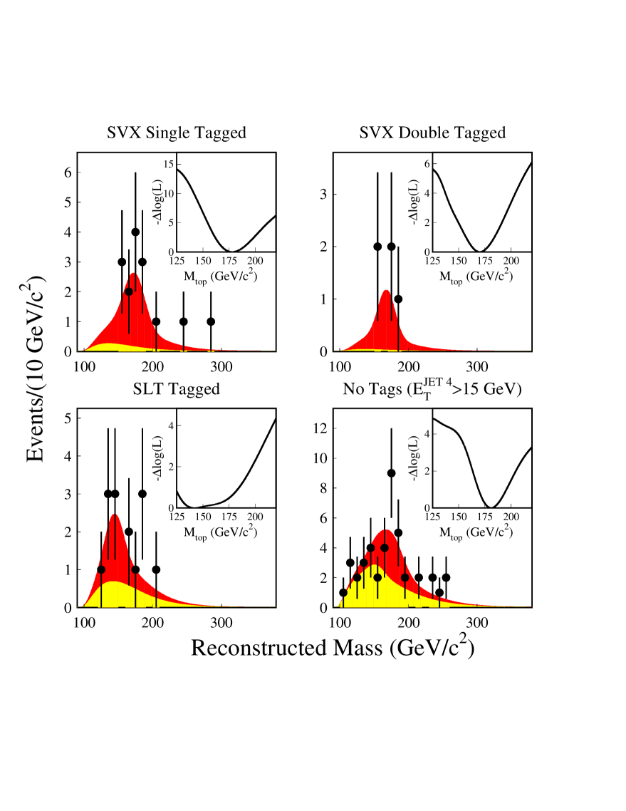
Fig. 36.: The CDF top quark mass distributions for the four lepton+jets subsamples. The points are the data, the heavily shaded area is the top signal + background combination resulting from the fit, and the lightly shaded area is background alone. The insets show the negative log likelihood vs. $m_{t}$ for each subset. From Ref. [cdftopmass98].

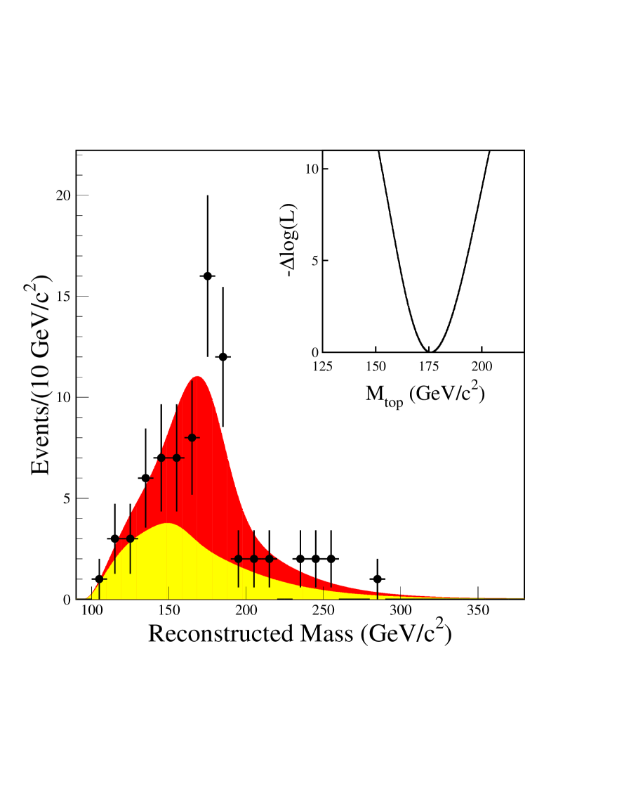
Fig. 37.: The CDF top quark mass distribution for all four subsamples combined. The points are the data, the heavily shaded area is the top signal + background combination resulting from the fit, and the lightly shaded area is background alone. The inset shows the negative log likelihood vs. $m_{t}$. From Ref. [cdftopmass98].

6.2.3 All Jets Channel

CDF has also presented a top quark mass measurement in the challenging all-jets channel,[cdfalljets] in which both $W$ bosons decay hadronically. The event sample is based on the kinematic cuts of technique I of the cross section measurement (see Sec. 5.2.3), except that six jets are required and the cut on $H_{T}=\sum E_{T}^{\text{jet}}$ is relaxed from $300~{}\text{GeV}$ to $H_{T}>200~{}\text{GeV}$. The latter change is to reduce the bias in the mass distributions due to threshold effects. Before requiring a $b$-tag, 1121 events survive these cuts. After tagging, 136 events remain.

CDF obtains a fitted mass for each event using a kinematic fit to the hypothesis $t\overline{t}\rightarrow(bW^{+})(\overline{b}W^{-})\rightarrow(bq\overline{q})(\overline{b}q\overline{q})$. One can parameterize these events so that there are thirteen unknowns (the top quark mass and the three-momenta of both top quarks and $W$ bosons) and sixteen constraints (four-momentum conservation at both top quark and $W$ boson decay vertices). Thus, a 3C fit is possible. As in the kinematic fit in the lepton + jets channel, CDF tries all possible assignments of jets to the quarks which are consistent with assigning the tagged jet as a $b$-jet. The fit which gives the smallest $\chi^{2}$ is retained. Figure 38 shows the resulting three-jet fitted mass distribution.

A major challenge for this analysis is the background estimation. This is because not only is the background large, but its fitted mass distribution is not that different in shape from the signal (see Fig. 38). Therefore, an error in the background normalization could result in a bias in the mass measurement. CDF estimates the background using a technique similar to that used for the lepton+jets and all-jets cross section measurements: each jet in the sample of 1121 untagged events is weighted by the probability for a jet in multijet events to be tagged. This tag probability is parameterized in terms of the jet $E_{T}$, $\eta$, and track multiplicity and the event aplanarity. This technique yields an estimated background of $108\pm 9$ events. The shape of the fitted mass distribution is taken directly from the untagged sample.

The final mass estimate is extracted from the fitted mass distribution using a maximum likelihood fit based on discrete templates (similar to what was used in the discovery paper[cdfdiscovery]). The result is $186\pm 10~{}\text{GeV}/c^{2}$ (see Fig. 38). In the published reference,[cdfalljets] CDF quotes a systematic uncertainty due to the modeling of gluon radiation and fragmentation effects of $\pm 8.6~{}\text{GeV}/c^{2}$. However, this uncertainty was recently revised downwards[roser] to $\pm 3.0~{}\text{GeV}/c^{2}$. The uncertainty due to the jet energy scale is $\pm 5.4~{}\text{GeV}/c^{2}$. Other systematic uncertainties are due to the fitting method ($\pm 5.2~{}\text{GeV}/c^{2}$) and the background estimation method ($\pm 1.7~{}\text{GeV}/c^{2}$). When these are combined in quadrature, one obtains a total systematic uncertainty of $\pm 8.2~{}\text{GeV}/c^{2}$.

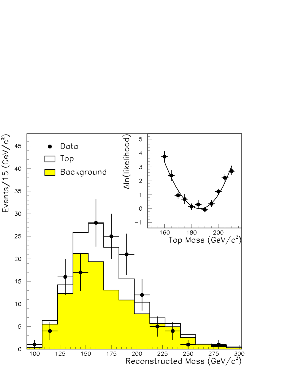
Fig. 38.: The CDF fitted mass distribution for the all jets sample. The points are the data, the shaded histogram is the background, and the open histogram is the sum of $t\overline{t}$ signal with $m_{t}=175~{}\text{GeV}/c^{2}$ and background. The inset shows the log-likelihood curve. From Ref. [cdftopmass98].

6.3 DØ Analyses

The DØ collaboration has measured the top quark mass in both the dilepton and lepton+jets channels.

6.3.1 Dilepton Channel

A dilepton $t\overline{t}$ event is kinematically underconstrained due to the two unobserved neutrinos. This would seem to preclude the use of kinematic fits as a means to estimate the top quark mass. However, Kondo [kondo88] and Dalitz and Goldstein [dalitz92a] have shown that it is possible to estimate the mass from an ensemble of kinematic fits by making use of additional information concerning the likelihood of given final states. These suggestions were pursued vigorously by DØ and led to a successful measurement of the top quark mass in these channels.[d0llmass, d0llmassprd]

The DØ collaboration has five dilepton candidate events (3 $e\mu$, 1 $ee$, and 1 $\mu\mu$) after applying the selection criteria used in the cross section measurement. An additional $ee$ event is selected by relaxing the track requirement on one of the electrons in the presence of a semileptonic (soft muon) $b$-tag. These six events are used to measure the top quark mass.[d0llmass, d0llmassprd] The expected backgrounds are $0.21\pm 0.16$, $0.47\pm 0.09$, and $0.73\pm 0.25$ events in the $e\mu$, $ee$, and $\mu\mu$ channels, respectively.

The invariant mass constraints $m(\ell_{1}\nu_{1})=m(\ell_{2}\nu_{2})=M_{W}$ and $m(\ell_{1}\nu_{1}b_{1})=m(\ell_{2}\nu_{2}b_{2})$ depend on the unknown neutrino four-vectors, $\nu_{1}$ and $\nu_{2}$. But, given a value for the top quark mass $m_{t}$, the system can be solved to within a four-fold ambiguity. The crucial observation is that not all hypotheses about the value of the top quark mass are equally probable: some final-state kinematic configurations are more likely than others, and so some top quark masses are preferred over others. Therefore, if one could assign such probabilities given the measured momenta, it would be possible to estimate the top quark mass. For an assumed value of $m_{t}$, DØ assigns a probability $p(D|m_{t})$ to the measured momenta $D$ and uses Bayes’ theorem,[bayes]

$$p(m_{t}|D)=\frac{p(D|m_{t})p(m_{t})}{\int_{0}^{\infty}p(D|m_{t}^{\prime})p(m_{t}^{\prime})\;dm_{t}^{\prime}},$$ (22)

to compute the probability $p(m_{t}|D)$ of $m_{t}$ given the fourteen measured parameters comprising the data $D$. The expression $p(m_{t})$ is the prior probability for $m_{t}$.

For each value of $m_{t}$, there are up to four possible solutions per jet-to-parton assignment, or configuration. For each solution and configuration, a likelihood $L$ is computed. These likelihoods are summed over all solutions and configurations to arrive at the overall likelihood $p(D|m_{t})$. DØ chooses the prior probability for $m_{t}$ to be flat, so that Eq. (22) reduces to $p(m_{t}|D)\propto p(D|m_{t})$.

In principle, the likelihood can be computed analytically, using

$$p(D|m_{t})\propto\int f(x)f(\bar{x})|{\cal M}|^{2}r(D|{\bf v})\delta^{4}\;d^{18}{\bf v}.$$ (23)

Here, ${\bf v}$ is the set of eighteen parameters needed to completely specify the kinematics of the event, ${\cal M}$ is the matrix element for the process $q\overline{q}\rightarrow t\overline{t}+X\rightarrow\ell^{+}\nu b\ell^{-}\bar{\nu}\overline{b}$, and $f(x)$ and $f(\bar{x})$ are the parton densities for quarks and antiquarks of momentum fractions $x$ and $\bar{x}$ in the proton and antiproton, respectively. The detector resolution function $r(D|{\bf v})$ gives the probability to observe the data $D$ given the true kinematic configuration ${\bf v}$. The four-dimensional delta function $\delta^{4}$ enforces the kinematic constraints:

$$\delta^{4}=\delta(m(\ell^{+}\nu)-M_{W})\delta(m(\ell^{-}\bar{\nu})-M_{W})\delta(m(\ell^{+}\nu b)-m_{t})\delta(m(\ell^{-}\bar{\nu}\overline{b})-m_{t}).$$ (24)

Unfortunately, it is not feasible to evaluate this expression for the large number of Monte Carlo events which are used to construct the templates. Therefore, DØ computes only much simplified approximations to this full likelihood. Two different methods are employed for doing so, as discussed below.

The first method, called matrix element weighting (${\cal M}$WT), is a modified version of the procedure suggested by Dalitz and Goldstein.[dalitz92a] Here, the sum of the transverse momenta of the two neutrinos is required to be equal to the measured ${\hbox{$E$\kern-6.00006pt\lower-0.43057pt\hbox{/}}}_{T}$. The system is then solved for the neutrino momenta, and hence the top and antitop four-vectors. The likelihood for a given solution and configuration $j$ is taken to be

$$L(D|m_{t},j)\propto f(x)f(\bar{x})P(E_{{\ell}1}^{CM}|m_{t})P(E_{{\ell}2}^{CM}|m_{t}),$$ (25)

where $f(x)$ and $f(\bar{x})$ are again the parton distribution functions (DØ uses CTEQ3M[cteq95]) and $P(E_{\ell}^{CM}|m_{t})$ is the probability density for the lepton energy in the rest frame of the top quark, $E_{\ell}^{CM}$.

In the second method, called the neutrino weighting ($\nu$WT) method, for each configuration $j$, the expected phase space of neutrino pseudorapidity in $t\overline{t}$ events (at a given $m_{t}$) is divided into elements with equal phase space weight. For each pair of neutrino $\eta$ values, a solution is sought. If a solution is found, the likelihood $L(D|m_{t},j)$ is assigned based on the degree to which the sum of the neutrino transverse momenta agrees with the ${\hbox{$E$\kern-6.00006pt\lower-0.43057pt\hbox{/}}}_{T}$ in the event. For this calculation, only the smearing due to the underlying event is taken into account. For both methods, one sums $L$ over all solutions and configurations to obtain $p(D|m_{t})$, and hence $p(m_{t}|D)$.

So far, we have not accounted for the detector resolution function, $r(D|d)$, where $d$ are the true values of the momenta. (The information in $d$ is a subset of that in ${\bf v}$.) To include the effects of $r$, DØ uses the true, rather than the measured, momenta to solve the system. But since the true momenta are unknown, it is necessary to consider all possible values of the true momenta $d$, constrained (probabilistically) by the measured momenta $D$, which of course are fixed. (In Ref. [d0llmass], it is stated that the measured momenta are “smeared,” but this we regard as physicists’ argot for the statement we have just made.) The measured momenta $D$ and the true momenta $d$ are related via the experimental resolution function $r(D|d)$, which modifies the relationship between $p(D|m_{t})$ and $L(d|m_{t},j)$ (now written in terms of the true momenta $d$) thus:

$$p(D|m_{t})\propto\int_{d}r(D|d)\sum_{j}L(d|m_{t},j),$$ (26)

where the integration is over all possible momenta. DØ models its jet resolution function by a double Gaussian, which accounts for the inherent energy resolution of the DØ calorimeter plus the effects of large angle gluon radiation. The ${\hbox{$E$\kern-6.00006pt\lower-0.43057pt\hbox{/}}}_{T}$ is computed from the true momenta plus the contribution from the underlying event. The latter is included by fluctuating each component of ${\hbox{$E$\kern-6.00006pt\lower-0.43057pt\hbox{/}}}_{T}$ with a Gaussian, with a standard deviation of $4~{}\text{GeV}$.

Because of initial or final state radiation (ISR or FSR), an event may have more than two jets. In that case, DØ considers all possible interpretations of the jets, merging jets classified as FSR with the appropriate $b$-jet. Each interpretation is assigned a weight, which is the product of the weights assigned to each jet. Therefore, for events with three or more jets, the sum in Eq. (26) becomes a weighted sum. The weight assigned to an ISR jet is $\exp(-E_{T}\sin\theta/(25~{}\text{GeV}))$, where $\theta$ is the polar angle of the ISR jet. For an FSR jet coming from a $b$-quark, which together with the $b$-jet form an invariant mass $m$, the weight assigned is $\exp(-m/(20~{}\text{GeV}/c^{2}))$.

The normalized distributions of $p(D|m_{t})$ for the six candidate events are shown in Fig. 39. If the background in this sample of six events were negligible and no approximations were made in computing $p(D|m_{t})$, one could simply form the product of the six distributions and use the position of its peak or its mean as an estimate of the top quark mass. However, the background cannot be neglected, and the effects of the approximations must be taken into account. Therefore, DØ performs a maximum likelihood fit to a sum of signal and background templates. The signal templates are constructed from Monte Carlo simulations, the background templates from a combination of Monte Carlo and data.

Fig. 39.: Distributions of $p(D|m_{t})$ for the six DØ dilepton candidates, using the ${\cal M}$WT (dashed) and $\nu$WT (solid) methods. From Ref. [d0llmass].

To make use of the information contained in the shape of the distributions $p(m_{t}|D)$, the latter are normalized and divided into five bins of width $40~{}\text{GeV}/c^{2}$ (see Fig. 40). For each event $i$, the integrated content of each of the first four bins form the components of a four-dimensional vector $\bar{w}_{i}$. Only four bins are used because the content of the fifth bin is determined by the normalization condition, and is therefore not independent. The likelihood function is then

$${\cal L}(\bar{w}|m_{t},n_{s},n_{b})=G(\bar{n_{b}}|n_{b})\;P(N|n_{s}+n_{b})\prod_{i}^{N}\frac{n_{s}f_{s}(\bar{w}_{i}|m_{t})+n_{b}f_{b}(\bar{w}_{i})}{n_{s}+n_{b}},$$ (27)

where $n_{s}$ and $n_{b}$ are the mean signal and background counts, $G(\bar{n_{b}}|n_{b})$ is a Gaussian constraint on $n_{b}$, $P(N|n_{s}+n_{b})$ is a Poisson constraint on $(n_{s}+n_{b})$ to the observed sample size $N=6$, and $f_{s}$ and $f_{b}$ are four-dimensional probability density templates for the signal and background, respectively. These templates are approximated using a multivariate probability density method.[holmstroem95] The maximum likelihood estimate of $m_{t}$ and its error are determined by a quadratic fit to the $-\ln\cal{L}$ curve, using nine points about the minimum.

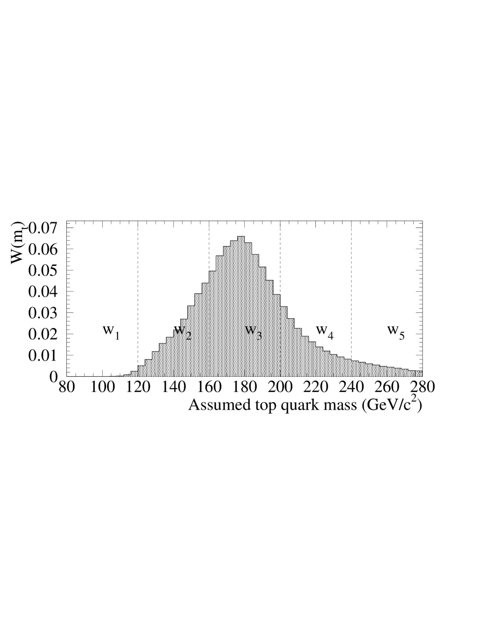
Fig. 40.: The likelihood curve for a typical Monte Carlo $t\overline{t}$ event, normalized to unity. The vertical lines show the five bins into which the likelihood is divided. From Ref. [d0llmassprd].

The sums of the weights for the six candidate events in the five mass bins are compared with the signal and background expectations in Fig. 41. The insets show the $-\ln\cal{L}$ distributions from which the estimates $m_{t}=168.2\pm 12.4~{}\text{GeV}/c^{2}$ ($\cal M$WT) and $m_{t}=170.0\pm 14.8~{}\text{GeV}/c^{2}$ ($\nu$WT) are extracted. Table 14 shows the results of fits to subsamples of the data. As shown in Table 15, the total systematic uncertainty is estimated to be $3.6~{}\text{GeV}/c^{2}$, dominated by the jet energy scale uncertainty. DØ combines the results from the $\cal M$WT and $\nu$WT analyses, taking into account the $77\%$ correlation between them, to obtain $m_{t}=168.4\pm 12.3~{}\text{(stat)}\pm 3.6~{}\text{(syst)}~{}\text{GeV}/c^{2}$.

Fig. 41.: The sum of the normalized candidate likelihoods for the ${\cal M}$WT (left) and $\nu$WT (right) analyses, compared to the results of the maximum likelihood fit. The solid histogram is the best-fit $t\overline{t}$ signal plus background, and the dotted histogram is background alone. The insets show the $-\ln{\cal L}$ as a function of $m_{t}$. From Ref. [d0llmass].

Table 14.: Summary of DØ’s dilepton $m_{t}$ measurements for full and partial data sets. Uncertainties are statistical only. From Ref. [d0llmass].

Channels Fit	${\cal M}$WT ($\text{GeV}/c^{2}$)	$\nu$WT ($\text{GeV}/c^{2}$)
$e\mu$ + $ee$ + $\mu\mu$	$168.2\pm 12.4$	$170.0\pm 14.8$
$e\mu$ + $ee$	$168.0\pm 12.7$	$173.3\pm 14.0$
$e\mu$	$173.1\pm 13.3$	$170.1\pm 14.5$

Table 15.: Systematic errors for DØ’s measurement of $m_{t}$ in the dilepton channels. From Ref. [d0llmass].

Source	Error ($\text{GeV}/c^{2}$)
Jet energy scale	2.4
Signal model	1.8
Multiple interactions	1.3
Background model	1.1
Likelihood fit	1.1
Total	3.6

6.3.2 Lepton+Jets Channels

The distributions of fitted mass ($m_{\text{fit}}$) for signal and background can overlap significantly, depending on the mass of the top quark. Therefore, in order to extract the top quark mass reliably from an $m_{\text{fit}}$ distribution, it is necessary either to suppress the background sufficiently or to make optimal use of available information. Requiring the presence of $b$-jets, as we have seen, is a simple and effective means of enhancing the signal to background ratio. However, DØ uses only soft-lepton tagging, for which the tagging efficiency is only $\approx 20\%$ in $\text{lepton}+\geq 4~{}\text{jets}$ events, compared to $\approx 53\%$ at CDF, which has the ability to tag $b$-jets with the SVX.

It is therefore noteworthy that in spite of DØ’s relatively poorer $b$-tagging, it has managed to measure the top quark mass with a precision approaching that of CDF.[d0ljtopmassprd, d0ljmassprl] DØ achieves this by using multivariate techniques[pushpadpf, pushpapbarp, strovink95] for separating signal and background while minimizing the correlation of the selection with the top quark mass. Two multivariate methods are used to compute, approximately, a signal probability $p(\text{top}|D)$ for each event, given data $D$. A likelihood fit of the data to a discrete set of signal and background models in the $(p(\text{top}|D),m_{\text{fit}})$ plane is performed to extract the top quark mass.

The event selection is based on that used for the cross section measurement (see Sec. 5.3.2), with the following differences:

• Four jets (with $E_{T}>15~{}\text{GeV}$ and $|\eta|<2.0$) are always required.

• The aplanarity and $H_{T}$ cuts are not applied.

• Events containing high-$p_{T}$ photons or more than one high-$p_{T}$ electron are rejected.

These cuts select 91 events, of which seven are tagged. The dominant background is $W+\text{jets}$, and about $20\%$ of the background comes from QCD multijets with a fake lepton.

The events are analyzed using a kinematic fit to the $t\overline{t}\rightarrow\ell\nu b\overline{b}q\overline{q}$ hypothesis. As in the CDF lepton+jets mass analysis, the jets are first corrected to match the partons, and the fit is then tried for all possible jet configurations consistent with the $b$-tagging information. For each fit, this gives a fitted mass $m_{\text{fit}}$ and a fit $\chi^{2}$. The jet configuration with the lowest $\chi^{2}$ is retained, and events are required to have this minimum $\chi^{2}<10$. After this final cut, 77 events survive, of which five are tagged.

The kinematic fit is tested on $t\overline{t}$ Monte Carlo samples both with and without QCD evolution and gluon radiation, together with the simulation of detector effects. The $m_{\text{fit}}$ distributions from these tests are shown in Fig. 42. The $m_{\text{fit}}$ distribution at the partonic level, without QCD evolution, shows a very sharp peak (with $\sim 2.4~{}\text{GeV}/c^{2}$ width). About 80% of the time the configuration with the lowest $\chi^{2}$ is the correct one. The width of the peak is mainly due to the widths of $W$ bosons. Like CDF, DØ finds that, after QCD evolution and fragmentation effects are included, the width of the $m_{\text{fit}}$ distribution grows to $\sim 26~{}\text{GeV}$. (The jets are reconstructed by clustering particles in a cone of width $R=0.5$.) With these effects included, the correct configuration is selected only about 40% of the time. The reduction in the selection efficiency is due to the confusion arising from the splitting and merging of jets, the jet finding efficiencies, and increased jet combinatorics. Including detector effects does not change the width appreciably (see Fig. 42c). It can therefore be concluded that the primary contribution to the width of the mass distribution is from the extra gluon radiation and jet combinatoric effects, rather than from the detector resolution.

Fig. 42.: Monte Carlo distributions of fitted mass for herwig $t\overline{t}$ events with $m_{t}=170~{}\text{GeV}/c^{2}$, showing how radiation and detector resolution affect the width of the mass distribution. The hatched histograms show the results when the correct jet configuration is used (regardless of whether or not it has the lowest $\chi^{2}$). The means and widths are from the Gaussian fits shown by the dashed lines. (a) Using herwig partons directly, no radiation or detector effects. (b) Using final state Monte Carlo particles clustered into cones. Includes the effects of radiation, but not detector effects. (c) After full detector simulation and reconstruction. From Ref. [d0ljtopmassprd].

For the cross section analysis, much of the discrimination between signal and background is achieved through the use of the variable $H_{T}$. However, this variable is not usable for the mass measurement because it is highly correlated with the top quark mass. Therefore, making significant cuts on $H_{T}$ reduces the sensitivity to $m_{t}$. In light of this, DØ embarked on an extensive search for variables that provide good discrimination between signal and background and are weakly correlated with $m_{\text{fit}}$. This resulted in the following four variables:

• $x_{1}\equiv\mbox{${\hbox{$E$\kern-6.00006pt\lower-0.43057pt\hbox{/}}}_{T}$}$.

• $x_{2}\equiv\cal A$, the event aplanarity, as defined earlier.

• $x_{3}\equiv(H_{T}-E_{T}^{\text{jet}1})/H_{z}$, where $H_{T}=\sum E_{T}$ of all selected jets and $H_{z}\equiv\sum|E_{z}|$ of all objects in the event (lepton, neutrino, and the jets), $E_{z}$ being the momentum component of the object in the beam direction. This variable measures the centrality of the event.

• $x_{4}\equiv\Delta R_{jj}^{\min}\cdot E_{T}^{\min}/(E_{T}^{\ell}+\mbox{${\hbox{$E$\kern-6.00006pt\lower-0.43057pt\hbox{/}}}_{T}$})$, where $\Delta R_{jj}^{\min}$ is the minimum $\Delta R$ of the six pairs of four jets and $E_{T}^{\min}$ is the smaller jet $E_{T}$ from the minimum $\Delta R$ pair. This variable measures the extent to which the jets are clustered together.

The distributions of these variables for signal and background are plotted in Fig. 43. We see that, on average, the signal events have larger values of the variables than do the background events. But, we also note that, while each variable provides some discrimination, none is decisive; one might anticipate that direct cuts on the variables may not be the most effective way to use them. It proves to be more effective to treat the variables collectively and cut on a single multivariate discriminant ${\cal D}(x)=s(x)/[s(x)+b(x)]$, where $s(x)$ and $b(x)$ are the signal and background densities. Two multivariate methods are used to approximate ${\cal D}(x)$: (1) a log-likelihood technique, referred to as the low bias (LB) method (due to the small correlation of the discriminant with the fitted mass), and (2) a feed-forward neural network (NN). In the LB method, DØ parameterizes the ratios $L_{i}(x_{i})=s_{i}(x_{i})/b_{i}(x_{i})$, where $s_{i}$ and $b_{i}$ are the signal and background densities for variable $x_{i}$. Then one computes $L=\prod_{i}L_{i}^{w_{i}}$ and ${\cal D}_{\text{LB}}=L/(1+L)$ for each event. The weights $w_{i}$ are adjusted to minimize the correlation between the discriminant and the fitted mass. The NN method, by construction, takes into account all correlations between the variables used. A three layer feed-forward neural network, with four input nodes, five hidden nodes, and one output node is trained on samples of Monte Carlo $t\overline{t}$ ($m_{t}=170~{}\text{GeV}/c^{2}$) and background events. The neural network is trained using the back-propagation algorithm, choosing the output to be unity for the signal and zero for the background. For a given event, the network output ${\cal D}_{\text{NN}}$ directly approximates the ratio $s(x)/[s(x)+b(x)]$. Figure 44 shows that ${\cal D}_{\text{LB}}$ and ${\cal D}_{\text{NN}}$ are distributed as predicted and provide comparable discrimination. As expected, the signal peaks near unity and the background near zero.

Fig. 43.: DØ distributions of the discriminant variables $x_{1}$, $x_{2}$, $x_{3}$, and $x_{4}$ (see text for definitions) for signal (solid histograms) and for background (dashed histograms). All histograms are normalized to unity.

Fig. 44.: Top: DØ distributions of ${\cal D}_{\text{LB}}$ and ${\cal D}_{\text{NN}}$ for signal (hatched, $m_{t}=175~{}\text{GeV}/c^{2}$) and background (open). The histograms are normalized to unity. Bottom: The distributions of ${\cal D}_{\text{LB}}$ and ${\cal D}_{\text{NN}}$ for data (histogram), compared to the predicted signal plus background (filled circles) and background alone (open triangles). The normalization is from the result of the likelihood fit. From Ref. [d0ljtopmassprd].

DØ carries out two analyses, based on the ${\cal D}_{\text{LB}}$ and ${\cal D}_{\text{NN}}$ discriminants. The data are binned in the $({\cal D}_{\text{LB/NN}},m_{\text{fit}})$ space. Both analyses use the same binning for $m_{\text{fit}}$ (20 bins, over the range 80–$280~{}\text{GeV}/c^{2}$), but differ in how the discriminant is binned. For the ${\cal D}_{\text{LB}}$ analysis, the events are split into two bins, depending on whether or not they pass the “LB cut,” defined by ${\cal D}_{\text{LB}}>0.43$ and $H_{T}-E_{T}^{\text{jet}1}>90~{}\text{GeV}/c^{2}$. (The latter condition removes mostly background; it does not affect the signal much.) For the NN analysis, the events are split into ten discriminant bins, as illustrated in Fig. 45.

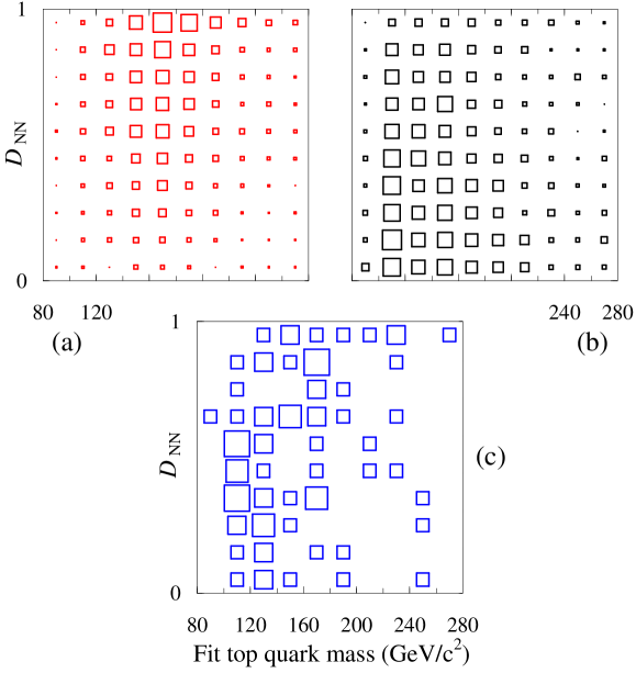
Fig. 45.: Events per bin ($\propto$ areas of boxes) in the $({\cal D}_{\text{NN}},m_{\text{fit}})$ plane for the DØ NN top mass analysis. (a) Expected top quark signal ($m_{t}=172~{}\text{GeV}/c^{2}$). (b) Expected background. (c) Data. From Ref. [d0ljmassprl].

For each method, a top quark mass is extracted from the binned data using a likelihood fit to a discrete set of signal and background templates. The likelihood function, based on Poisson statistics, is derived by a Bayesian method.[bayesplb] In this fit, the number of background events is left unconstrained. Figure 46 shows the results of the fits and the negative log-likelihoods, as functions of the top quark mass. For the LB method, the fit yields $m_{t}=174.0\pm 5.6\ \text{(stat)}~{}\text{GeV}/c^{2}$ and the number of background events $n_{b}=53.2_{-9.3}^{+10.7}$ (out of 77). For the NN method, the corresponding results are $m_{t}=171.3\pm 6.0\ \text{(stat)}~{}\text{GeV}/c^{2}$ and $n_{b}=48.2_{-8.7}^{+11.4}$. The total systematic uncertainty is estimated to be $5.5~{}\text{GeV}/c^{2}$ (see Table 16), of which $4.0~{}\text{GeV}/c^{2}$ comes from the jet energy scale uncertainty and $3.1~{}\text{GeV}/c^{2}$ from event modeling (including the modeling of initial and final state radiation in $t\overline{t}$ events).

Fig. 46.: Results from the DØ lepton+jets mass analysis. Bottom: The fitted mass distribution for events which pass the LB cut (a signal-rich sample). Upper left: The same, for events which fail the LB cut (a background-dominated sample). Upper right: The relative $-\ln{\cal L}$ functions for the two methods. From Ref. [d0ljmassprl].

Table 16.: Systematic uncertainties in the DØ lepton+jets top quark mass measurement.

Jet energy scale	$4.0~{}\text{GeV}/c^{2}$
Event modeling
$t\overline{t}$ signal	$1.9~{}\text{GeV}/c^{2}$
Background	$2.5~{}\text{GeV}/c^{2}$
Noise/Multiple Interactions	$1.3~{}\text{GeV}/c^{2}$
Monte Carlo statistics	$0.85~{}\text{GeV}/c^{2}$
Fit method	$1.3~{}\text{GeV}/c^{2}$
Total	$5.5~{}\text{GeV}/c^{2}$

DØ combines the LB and NN results, taking into account their mutual correlation of $88\%$, to get an overall measurement of $m_{t}=173.3\pm 5.6~{}\text{(stat)}\pm 5.5~{}\text{(syst)}~{}\text{GeV}/c^{2}$. For DØ, this result shows a marked improvement in precision with respect to the measurement published at the time of the discovery. This bodes well for the measurement of the top quark mass in Run 2 by both collaborations.

6.4 Summary of Mass Measurements

CDF observes 8 dilepton events with an estimated background of $1.3\pm 0.3$ events, and obtains a mass of $m_{t}=167.4\pm 10.3~{}\text{(stat)}\pm 4.8~{}\text{(syst)}~{}\text{GeV}/c^{2}$. In the lepton+jets channel, 76 events are observed, of which 15 are singly tagged and 5 doubly tagged with the SVX. The mass obtained from this sample is $175.9\pm 4.8~{}\text{(stat)}\pm 4.9~{}\text{(syst)}~{}\text{GeV}/c^{2}$. The 136-event all-jets sample, with a background of $108\pm 9$ events, yields $m_{t}=186\pm 10~{}\text{(stat)}\pm 8~{}\text{(syst)}~{}\text{GeV}/c^{2}$. Combining all the CDF measurements yields $m_{t}=175.3\pm 6.4~{}\text{GeV}/c^{2}$.

DØ observes 6 dilepton events with a background of $1.4\pm 0.3$ events, and measures a mass of $m_{t}=168.4\pm 12.3~{}\text{(stat)}\pm 3.6~{}\text{(syst)}~{}\text{GeV}/c^{2}$. In the lepton+jets channel, 77 events are observed (of which 5 are tagged), with an estimated background of $52\pm 9$ events. This gives $m_{t}=173.3\pm 5.6~{}\text{(stat)}\pm 5.5~{}\text{(syst)}~{}\text{GeV}/c^{2}$. When one combines the DØ dilepton and lepton+jets results, one obtains $m_{t}=172.1\pm 5.2~{}\text{(stat)}\pm 4.9~{}\text{(syst)}~{}\text{GeV}/c^{2}$.

Combining all five measurements yields[boaz] $m_{t}=173.8\pm 5.0~{}\text{GeV}/c^{2}$. The measurements, summarized in Fig. 47, are in striking agreement with each other as well as with the indirect measurements from precision electroweak data. It is remarkable that the top quark mass is now known to a precision (3%) that is far better than what was anticipated a few years ago!

Fig. 47.: Summary of all the top quark mass measurements from CDF and DØ.

7 Other Studies

7.1 Measurement of $|V_{tb}|$

The analyses discussed so far have assumed that the branching fraction of the decay $t\rightarrow Wb$ is essentially $100\%$. Clearly, we would like to be able to test this assumption.

The mixing between the three quark generations is described by the Cabibbo-Kobayashi-Maskawa (CKM) matrix:[cabibbo63]

$$\pmatrix{d^{\prime}\cr s^{\prime}\cr b^{\prime}\cr}=\pmatrix{V_{ud}&V_{us}&V_{ub}\cr V_{cd}&V_{cs}&V_{cb}\cr V_{td}&V_{ts}&V_{tb}\cr}\pmatrix{d\cr s\cr b\cr},$$ (28)

where the unprimed letters denote mass eigenstates and the primed ones denote weak eigenstates. The ratio $R$ of the branching fraction for a top quark decaying to a $b$-quark to that of a top quark decaying to any down-type quark $q$ can be written as

$$R={B(t\rightarrow Wb)\over B(t\rightarrow Wq)}={|V_{tb}|^{2}\over|V_{td}|^{2}+|V_{ts}|^{2}+|V_{tb}|^{2}}$$ (29)

(assuming that top quark decays to non-$W$ final states are negligible). In the Standard Model with three generations, the CKM matrix Eq. (28) must be unitary. With this constraint, current measurements imply that $0.9991<|V_{tb}|<0.9994$ ($90\%$ confidence level).[pdg96] If, however, the assumption of three generations is not made (while maintaining the unitarity of the expanded mixing matrix), then the $90\%$ confidence level interval for $|V_{tb}|$ opens up to $0.05<|V_{tb}|<0.9994$. Removing the unitarity assumption leaves $|V_{tb}|$ unconstrained. Therefore, if a measurement of $|V_{tb}|$ were to yield a result significantly different from unity, this would be indicative of new physics beyond the Standard Model (such as the presence of a fourth generation).

Table 17.: Data for the CDF $|V_{tb}|$ analysis from the lepton+jets (W4J) and dilepton (DIL) samples. From Ref. [tartarelli97].

Bin definition		Sample
SVX tags	SLT tags	W4J	DIL
none	none	126	6
none	one	14	—
one	—	18	3
two	—	5	0
Total		163	9

The CDF collaboration has made a preliminary measurement of $R$ using their combined lepton+jets and dilepton data samples.[tartarelli97, heinson97a] As shown in Table 17, CDF divides the data into several disjoint bins, depending on the observed $b$-tags. For each bin $i$, the number of events expected $n_{i}$ can be calculated as a function of the total numbers of signal and background events expected in the samples, the $b$-tagging efficiencies and fake rates, and $R$. These expectations $n_{i}$ are compared to the number of events actually observed in each bin $N_{i}$ using a likelihood function:

$${\cal L}=\prod_{i}P(N_{i}|n_{i}(\vec{x}))\prod_{j}G(x_{j}|\bar{x}_{j},\sigma_{j}),$$ (30)

where $P$ is the Poisson distribution $P(N|n)\equiv e^{-n}n^{N}/N!$. The quantities $x_{j}$ are other variables on which the predictions $n_{i}$ depend, each with a measured value $\bar{x}_{j}$ and uncertainty $\sigma_{j}$. They are convolved into the likelihood with a Gaussian function $G(x|\bar{x},\sigma)\propto\exp[(x-\bar{x})^{2}/2\sigma^{2}]$. A maximum likelihood fit is then performed to extract $R$ and the quantities $x_{j}$. For this fit, the number of top quarks in the samples is taken to be a free parameter, so that the result will not depend on the $t\overline{t}$ production cross section.

Fig. 48.: Variation of ${\cal L}$ as a function of $R$ (two different scales) for the CDF $|V_{tb}|$ measurement. From Ref. [tartarelli97].

The resulting likelihood is shown in Fig. 48. The fit yields $R=0.99\pm 0.29$. The uncertainty includes both statistical and systematic uncertainties, but is dominated by the statistical component. The $90\%$ and $95\%$ confidence limits for $R$ are, respectively, $R>0.64$ and $R>0.58$.

If three-generation unitarity is assumed, then the denominator in Eq. (29) is unity. The result then corresponds to $|V_{tb}|=0.99\pm 0.15$, or $|V_{tb}|>0.80$ and $|V_{tb}|>0.76$ at the $90\%$ and $95\%$ confidence levels, respectively. If the unitarity condition is relaxed, no statement can be made about $|V_{tb}|$ without further assumptions. CDF sets $|V_{td}|=0.009$ and $|V_{ts}|=0.04$, from the midpoint of their $90\%$ confidence levels determined with the unitarity assumption. The $90\%$ and $95\%$ confidence limits on $|V_{tb}|$ are then $|V_{tb}|>0.055$ and $|V_{tb}|>0.048$, respectively.

The dominant component of the systematic uncertainty on $R$ is the $b$-tagging efficiency. This is measured from the data with a precision limited by the available statistics of the control samples. Therefore, the total uncertainty on $R$ should decrease as $1/\sqrt{N}$ as statistics are increased. For a $2~{}\text{fb}^{-1}$ Run 2 at the Tevatron, the achievable precision for the $R$ measurement[tev2k] should be about $2\%$, corresponding to a $95\%$ CL limit of $|V_{tb}|>0.20$.

An alternate technique which should become possible in Run 2 is to measure $|V_{tb}|$ from single top production.[heinson97a] This will be discussed further in Sec. 8.3. We also note that it is possible to obtain indirect information on $|V_{tb}|$ from the precision measurements which have been made in the electroweak sector. A recent report [swain97] analyzes the $|V_{tb}|$ dependence of the single-loop corrections to the $Zb\overline{b}$ vertex. From a combined analysis using data from LEP, SLC, Tevatron, and neutrino scattering experiments, the authors derive $|V_{tb}|=0.77^{+0.18}_{-0.24}$, independent of unitarity assumptions.

7.2 Flavor-Changing Neutral Current Decays of the Top Quark

Flavor-changing neutral current (FCNC) decays can be used to probe for new physics at mass scales which are otherwise inaccessible. For example, the absence of the FCNC decay $K^{0}_{L}\rightarrow\mu^{+}\mu^{-}$ was indicative of the presence of the charm quark, even though the charm quark is several times heavier than the kaon.[gim] For the top quark, the SM rates for FCNC decays are very small,[eilam91] with the branching fractions $B(t\rightarrow cZ)$ and $B(t\rightarrow c\gamma)\sim 10^{-13}\text{--}10^{-12}$, $B(t\rightarrow cg)\sim 10^{-10}$, and $B(t\rightarrow cH)\sim 10^{-14}\text{--}10^{-13}$. Any observation of these decays at future experiments would therefore be evidence for new physics beyond the standard model.

Because of its large mass, the top quark provides a unique system in which to look for FCNC contributions. In many models, FCNC terms are suppressed by ratios of the quark masses to a weak interaction mass scale.[fritzsch89] Various models have been proposed in which the FCNC decays of the top quark are enhanced. These include models with two Higgs doublets,[eilam91] supersymmetry,[agashe95, yang97] and exotic fermions.[buchmuller89] These models typically predict increases of the FCNC decay rates of 3–4 orders of magnitude, which are still too small to be seen at any experiments planned in the near future. However, in supersymmetric models with baryon number nonconservation,[yang97] $B(t\rightarrow c\gamma)$ can be as large as $\approx 2\times 10^{-5}$, which could be observable at the upgraded Tevatron or the Large Hadron Collider, under construction at CERN.

Of particular interest are the decays $t\rightarrow c\gamma$ and $t\rightarrow cZ$, as they would yield the most distinctive final states.[han96] Indirect limits on these branching fractions may be derived from lower energy data; the results are $B(t\rightarrow c\gamma)<1\text{--}2\times 10^{-3}$ and $B(t\rightarrow cZ)<0.04$.

The CDF collaboration has searched for these decay modes[cdffcnc97] using their full Run 1 sample of $\approx 110~{}\text{pb}^{-1}$. The branching ratios are measured relative to a normalization sample, consisting of the tagged lepton+jets $t\overline{t}$ candidates. For the $t\rightarrow q\gamma$ mode, CDF uses two different cut definitions, depending on whether the $W$ boson (from the normally decaying top quark) decayed leptonically or hadronically. For the leptonic case, the requirements are a central lepton (either an electron or muon) with $p_{T}>20~{}\text{GeV}/c$, $\mbox{${\hbox{$E$\kern-6.00006pt\lower-0.43057pt\hbox{/}}}_{T}$}>20~{}\text{GeV}$, a photon with $p_{T}>20~{}\text{GeV}/c$, and at least two jets with $E_{T}>15~{}\text{GeV}$. A photon is identified from a cluster of energy in the electromagnetic calorimeter with no matching charged track. For the hadronic case, CDF requires a photon with $p_{T}>50~{}\text{GeV}/c$ and at least four jets with $E_{T}>15~{}\text{GeV}$, one of which must contain an SVX $b$-tag. In both cases, the invariant mass of one jet and the photon is required to lie in the range 140–$210~{}\text{GeV}/c^{2}$, consistent with the mass of the top quark. For the hadronic case, the tagged jet must be one of the remaining jets, and these remaining jets must satisfy $\sum E_{T}>140~{}\text{GeV}$, consistent with the decay of a second top quark. Acceptances relative to the SM decay mode are calculated using isajet and a parametric simulation of the CDF detector; the leptonic and hadronic cases constitute $60\%$ and $40\%$ of the acceptance, respectively. The expected backgrounds are less than half an event in each channel.

A single event is observed in the leptonic channel and none in the hadronic channel. The event is kinematically consistent with a $\overline{t}\rightarrow W^{-}\overline{b}\gamma$ decay, although the photon momentum ($p_{T}=88~{}\text{GeV}/c$) is quite large for this decay. CDF does not subtract the expected background, and thus the single observed event gives a branching fraction limit ($95\%$ CL) of:

$$B(t\rightarrow u\gamma)+B(t\rightarrow c\gamma)<3.2\%.$$ (31)

The systematic uncertainties in the acceptance calculation are dominated by the statistical uncertainty on the number of events in the normalization sample (34 candidates), followed by the uncertainty in the $b$-tagging efficiency.

For the $t\rightarrow qZ$ mode, CDF searches for the channel in which the $Z$ boson decays into a pair of leptons (electrons or muons) and the other top quark decays into three jets. The selection requirements are four jets with $E_{T}>20~{}\text{GeV}$ and $|\eta|<2.4$ and a pair of opposite-charge, same-flavor leptons with invariant mass in the range $75$–$105~{}\text{GeV}/c^{2}$. Acceptances are calculated as before; the total expected background is 1.2 events, with the major components being $Z+\text{multijet}$ production and $t\overline{t}$ dilepton decays where the lepton pair invariant mass is close to the $Z$ boson mass.

A single $Z\rightarrow\mu\mu$ event is observed, with event kinematics that are more consistent with $Z+\text{multijets}$ than with an FCNC top quark decay. Again, no background subtraction is performed, and the branching fraction limit ($95\%$ CL) is

$$B(t\rightarrow uZ)+B(t\rightarrow cZ)<33\%.$$ (32)

This search is less sensitive than the one for the $t\rightarrow q\gamma$ mode because of the small branching fraction of $Z$ bosons into charged leptons. The sources of systematic uncertainty are similar.

These limits can be improved during future Tevatron runs. For a $2~{}\text{fb}^{-1}$ Run 2, limits of $B(t\rightarrow q\gamma)<3\times 10^{-3}$ and $B(t\rightarrow qZ)<0.02$ are probably achievable.[tev2k]

7.3 Top Quark Decays to Charged Higgs

The minimal Standard Model contains a single complex Higgs doublet, giving rise to a single physical neutral Higgs scalar $H^{0}$. However, the form of the Higgs sector is not presently constrained by experiment, so it is interesting to consider models with an expanded Higgs sector. In particular, supersymmetric models require two Higgs doublets, one coupling to the up-type quarks and neutrinos, and the other coupling to the down-type quarks and charged leptons.[hhguide] In such theories, there are five physical Higgs bosons: two neutral scalars $H^{0}$ and $h^{0}$, a neutral pseudoscalar $A^{0}$, and a pair of charged scalars $H^{\pm}$. The relevant free parameters are the masses of the Higgs bosons and $\tan\beta$, the ratio of the vacuum expectation values of the neutral components of the two doublets.

If $m_{H^{+}}<m_{t}-m_{b}$, then the decay $t\rightarrow H^{+}b$ can occur, competing with $t\rightarrow W^{+}b$. The branching ratio is symmetric in $\log\tan\beta$ with a minimum at $\tan\beta=\sqrt{m_{t}/m_{b}}$. At the minimum, $B(t\rightarrow W^{+}b)\approx 100\%$, but the situation reverses for $\tan\beta\rightarrow 0$ or $\tan\beta\rightarrow\infty$, where $B(t\rightarrow H^{+}b)\approx 100\%$. See Fig. 49. The principal decays of $H^{+}$ are expected to be $H^{+}\rightarrow c\bar{s}$, dominant at low $\tan\beta$, and $H^{+}\rightarrow\tau^{+}\nu$, dominant at high $\tan\beta$. In addition, a recent paper [ma98] has pointed out that the virtual $t$ quark decay $H^{+}\rightarrow b\overline{b}W^{+}$ is important for $m_{H^{+}}\gtrsim 135~{}\text{GeV}/c^{2}$ and small $\tan\beta$. This is also illustrated in Fig. 49.

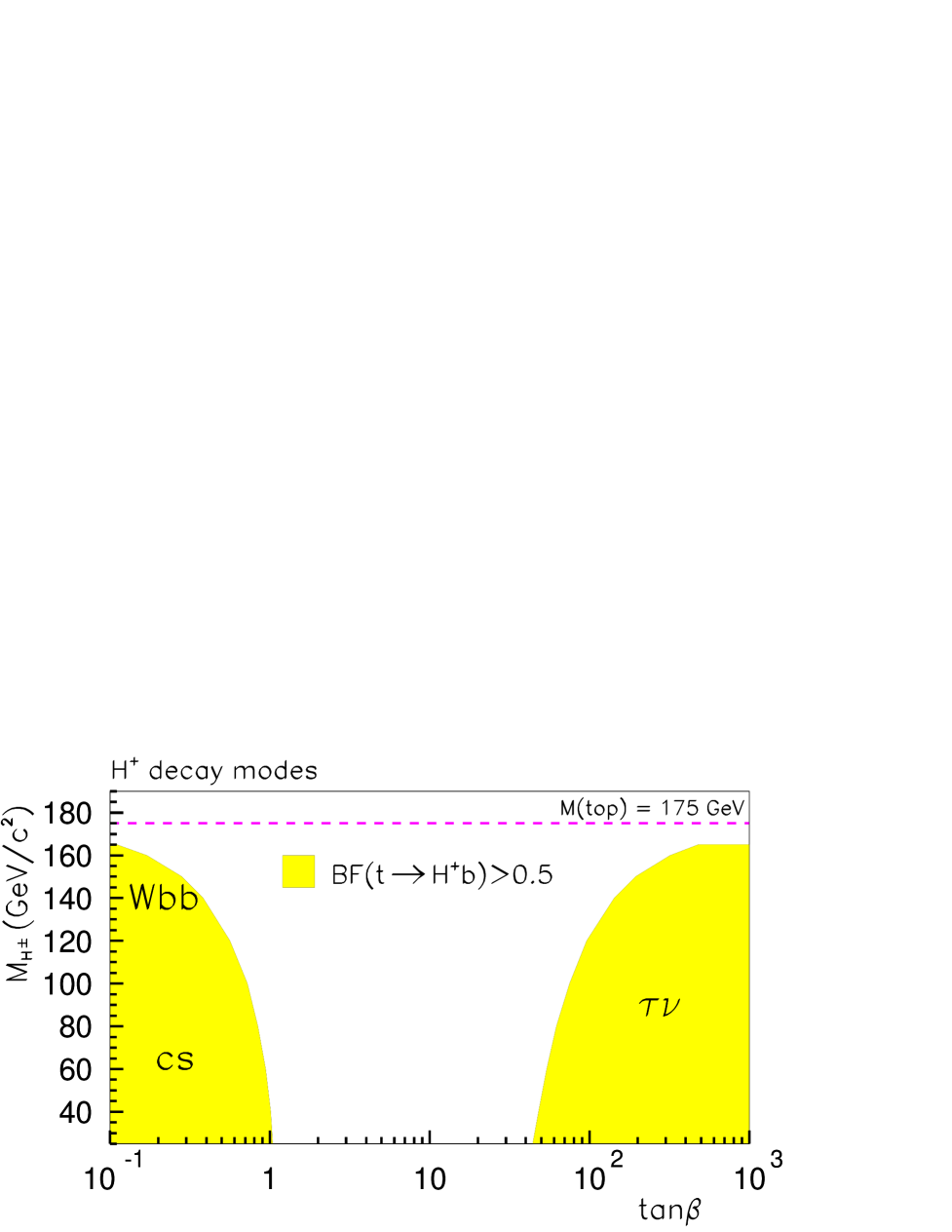
Fig. 49.: Regions in the $(m_{H^{+}},\tan\beta)$ plane where the branching ratio $B(t\rightarrow H^{+}b)>50\%$. At low $\tan\beta$, $H^{+}$ decays to $c\bar{s}$ and $b\overline{b}W^{+}$, with the latter mode dominating for $m_{H^{+}}>135~{}\text{GeV}/c^{2}$. At high $\tan\beta$, $H^{+}$ decays to $\tau^{+}\nu$. From Ref. [bevensee98].

It was also recently realized that there are problems with excluding very high and low values of $\tan\beta$. This is because the coupling of $H^{+}$ to fermions becomes arbitrarily large in these limits, causing the perturbative calculations of the branching ratios to break down. The widths of the Higgs boson and the top quark also become very large ($10$–$20~{}\text{GeV}/c^{2}$) in these regions. The $\tan\beta$ range over which the coupling is perturbative is approximately $0.2<\tan\beta<170$.

Some early limits on the charged Higgs mass are summarized in Ref. [barger90]. At present, the best limit independent of $\tan\beta$ is from LEP 2,[delphihiggs97] $m_{H^{+}}>54.5~{}\text{GeV}/c^{2}$ (95% CL), extending the LEP 1 limit[opalhiggs96] of $m_{H^{+}}>44.1~{}\text{GeV}/c^{2}$. (Preliminary results presented at the 1998 Moriond conference[dejong98] further extend this to $m_{H^{+}}>56.7~{}\text{GeV}/c^{2}$.) Limits at high $\tan\beta$ have been derived at the S$p\overline{p}\,$S [ua1higgs91] and from earlier Tevatron runs.[cdfhiggs96] A limit based on an independent analysis of CDF data is described in Ref. [guchait97], and an analysis of $\tau$ lepton decays which yields a limit on $m_{H^{+}}$ at large $\tan\beta$ is presented in Ref. [stahl97]. In addition, the CLEO collaboration, analyzing $b\rightarrow s\gamma$ decays and assuming a two-Higgs doublet extension of the Standard Model, derives a limit[cleopenguin95] of $m_{H^{+}}>[244+63/(\tan\beta)^{1.3}]~{}\text{GeV}/c^{2}$. However, models with additional structure, such as supersymmetry, can evade this limit.[goto96]

The CDF collaboration performs a direct search[cdfhiggs97] for $t\rightarrow H^{+}b$ in the large $\tan\beta$ region by looking for $H^{+}\rightarrow\tau^{+}\nu$, considering $t\overline{t}$ final states where either one or both top quarks decay via a Higgs boson. CDF requires one $\tau$ lepton with $p_{T}>10~{}\text{GeV}/c$, two jets with $E_{T}>10~{}\text{GeV}$, and one or more additional objects, either leptons (including $\tau$) or jets, with $p_{T}>10~{}\text{GeV}/c$. At least one of the jets must have an SVX $b$-tag. If the charged Higgs boson mass is close to the top quark mass, however, the $b$-jets may fall below the $E_{T}$ threshold. To regain acceptance for this case, CDF also considers a second (“$\tau\tau$”) final state, with no jet requirements but with two $\tau$ leptons with $p_{T}>30~{}\text{GeV}/c$. In addition, the two $\tau$ leptons must not be opposite in azimuth ($\Delta\phi_{\tau\tau}<160^{\circ}$). The $\tau$ identification algorithm used is similar to the calorimeter-based selection described in Sec. 3.3.4.

For both final states, it is required that $\mbox{${\hbox{$E$\kern-6.00006pt\lower-0.43057pt\hbox{/}}}_{T}$}>30~{}\text{GeV}$ and $\Delta\phi/(1^{\circ})+\mbox{${\hbox{$E$\kern-6.00006pt\lower-0.43057pt\hbox{/}}}_{T}$}/(1~{}\text{GeV})>60$, where $\Delta\phi$ is the distance in azimuth between the $\vec{\mbox{${\hbox{$E$\kern-6.00006pt\lower-0.43057pt\hbox{/}}}_{T}$}}$ and the closest other object. This cut removes events with mismeasured ${\hbox{$E$\kern-6.00006pt\lower-0.43057pt\hbox{/}}}_{T}$. In addition, any event containing a $e^{+}e^{-}$ or $\mu^{+}\mu^{-}$ pair with mass between 75 and $105~{}\text{GeV}/c^{2}$ is removed, in order to suppress background from $Z$ boson production.

In $100~{}\text{pb}^{-1}$ of data, CDF finds seven candidates passing the above cuts (six $\tau jjj$ events, one $\tau jje$ event, and no $\tau\tau$ events). The dominant source of background is fake $\tau$ leptons, estimated from jet data to be $5.4\pm 1.5$ events for both channels. Additional background sources, which can produce real $\tau$ leptons, include electroweak $W/Z+\text{multijet}$ processes and diboson production. These backgrounds are estimated using Monte Carlo simulations; the results are $1.9\pm 1.3$ and $0.08\pm 0.06$ events, respectively. The total background for both channels is thus $7.4\pm 2.0$ events, consistent with observation.

Acceptances are computed using isajet. The resulting exclusion contour is shown in Fig. 50 (left) for two different assumed top quark production cross sections. The lower of the two, $\sigma_{t\overline{t}}=5.0~{}\text{pb}$, corresponds to the theoretical prediction for a $m_{t}=175~{}\text{GeV}/c^{2}$ top quark,[laenen94] and the second is $50\%$ larger than that. For large $\tan\beta$, CDF excludes a charged Higgs boson with $m_{H^{+}}<147~{}\text{GeV}/c^{2}$ at the 95% confidence level. This limit can be extended by requiring that the product $\sigma_{t\overline{t}}B(t\overline{t}\rightarrow W^{+}bW^{-}\overline{b})$ be consistent with the (then current) CDF measured cross section[cdfdiscovery] of $6.8^{+3.6}_{-2.4}~{}\text{pb}$. The result is shown in Fig. 50 (right). Note that these limits may not be reliable for the nonperturbative region $\tan\beta>170$.

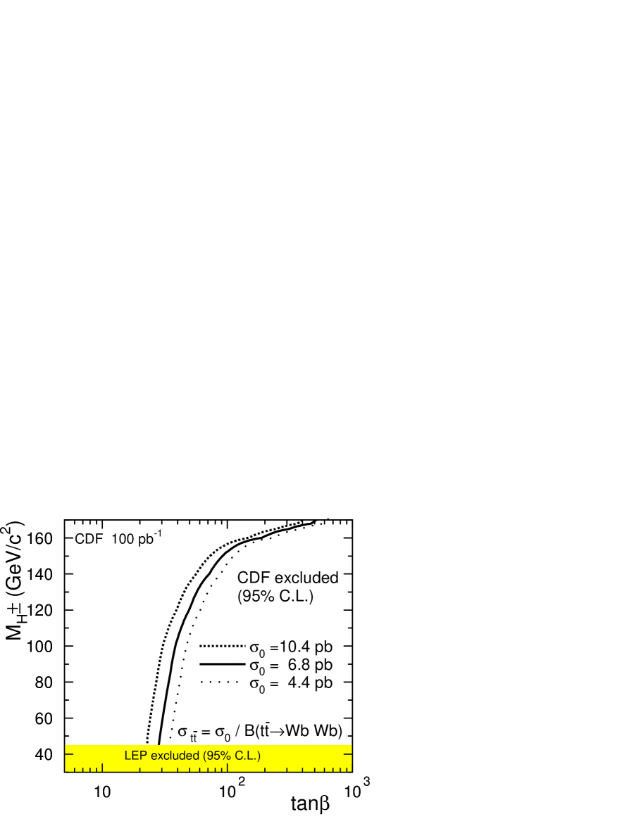
Fig. 50.: CDF charged Higgs exclusion region for $m_{t}=175~{}\text{GeV}/c^{2}$. The plot on the right adds the additional constraint $\sigma_{t\overline{t}}=\sigma_{0}/B(t\overline{t}\rightarrow W^{+}bW^{-}\overline{b})$. Note that these limits may not be reliable for the nonperturbative region $\tan\beta>170$. From Ref. [cdfhiggs97].

A second analysis strategy is the “indirect” search, which uses the results of the $t\overline{t}$ cross section and top quark mass measurements. It is based on the observation that the standard $t\overline{t}$ selection cuts are less efficient for $t\rightarrow H^{+}b$ than they are for $t\rightarrow Wb$. Therefore, if $t\rightarrow H^{+}b$ were to occur at a significant rate, there would be a shortfall in the measured cross section relative to the SM calculation. As an example, consider $m_{H^{+}}=70~{}\text{GeV}/c^{2}$ and $\tan\beta=0.4$ (with $m_{t}=175~{}\text{GeV}/c^{2}$ and $\sigma_{t\overline{t}}=5~{}\text{pb}$). With these parameters, one has $B(t\rightarrow H^{+}b)\approx 100\%$ and also $B(H^{+}\rightarrow c\bar{s})\approx 100\%$. Therefore, $t\overline{t}$ pairs will decay nearly always into a six-jet final state, containing neither a high-$p_{T}$ lepton nor any significant ${\hbox{$E$\kern-6.00006pt\lower-0.43057pt\hbox{/}}}_{T}$. The acceptance of the lepton+jets analyses for these events is practically zero, so all observed events must have been background. But the number of events actually observed is significantly above the background expectation; therefore, this point in the $(m_{H^{+}},\tan\beta)$ plane can be excluded at a high confidence level.

Both the CDF [bevensee98] and DØ [klima98] collaborations have carried out such an analysis. The results from CDF for the low $\tan\beta$ region are shown in Fig. 51. DØ uses this method in both the low and high $\tan\beta$ regions, as shown in Fig. 52. Note that the DØ results have not yet been updated to take into account the three body Higgs decay and the nonperturbative regions.

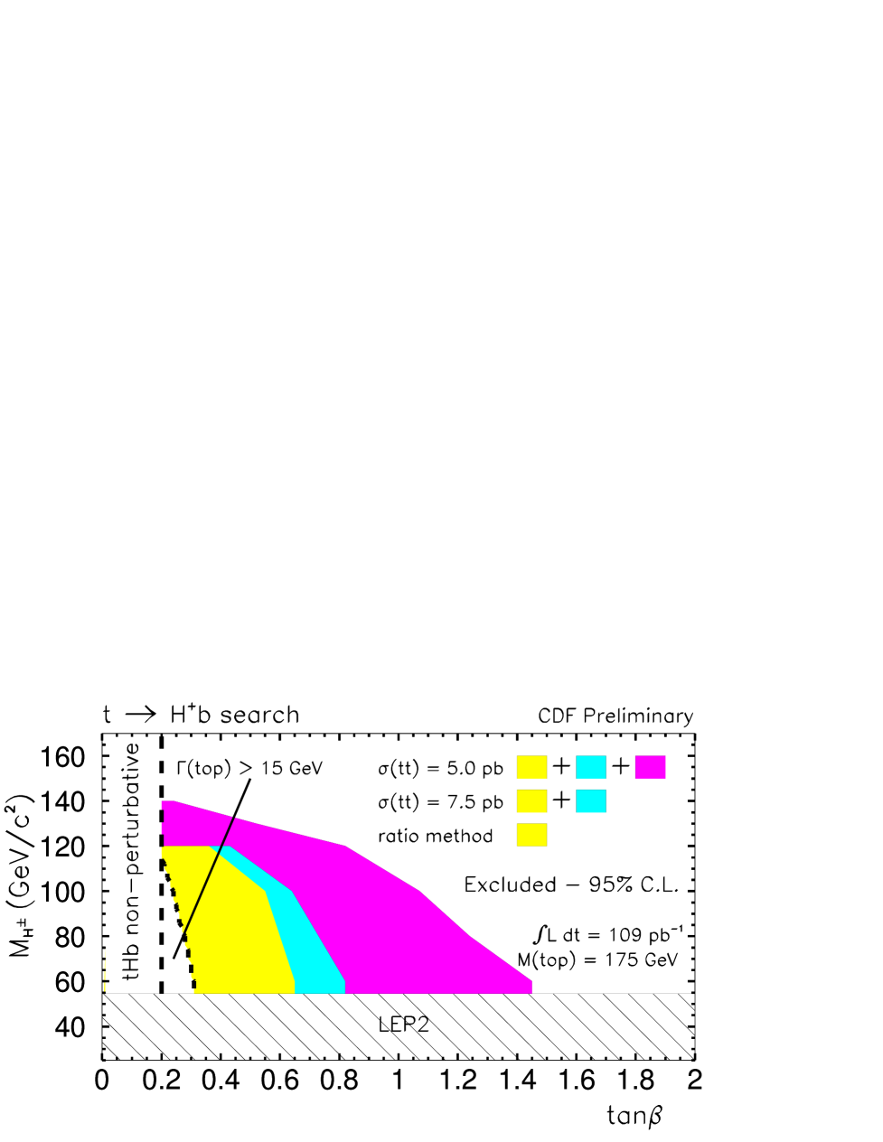
Fig. 51.: CDF 95% exclusion limit contours in the $(m_{H^{+}},\tan\beta)$ plane for the indirect Higgs boson search. Results are shown for two different assumed top quark cross sections. The region labeled “ratio method” is excluded by using the lepton + jets channel to measure $\sigma_{t\overline{t}}$, rather than assuming a value. The search does not apply in regions where $\tan\beta<0.2$ or where the top quark width is predicted to be larger than $15~{}\text{GeV}/c^{2}$. From Ref. [bevensee98].

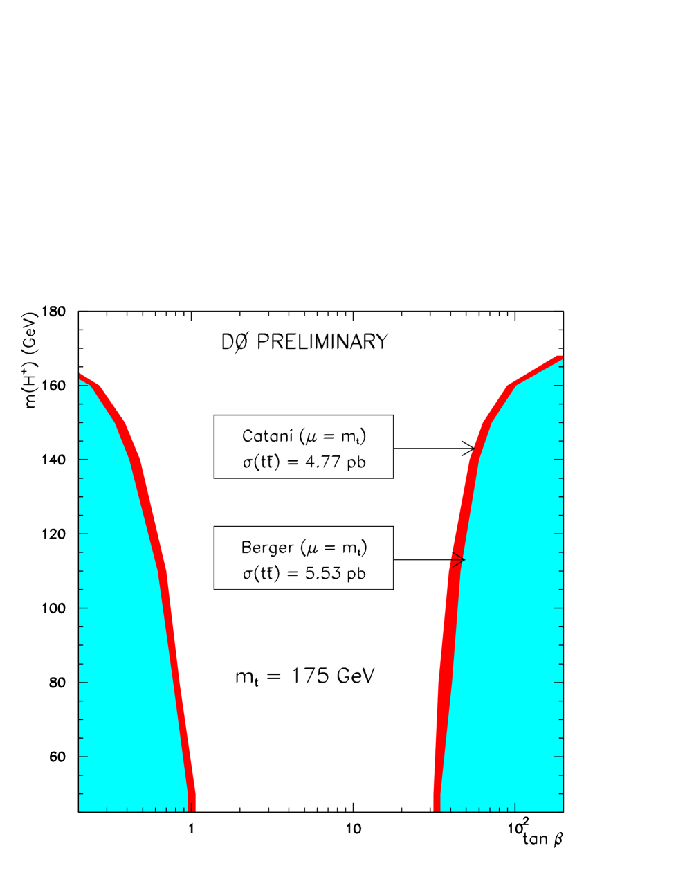
Fig. 52.: DØ 95% exclusion limit contours in the $(m_{H^{+}},\tan\beta)$ plane for the indirect Higgs boson search. This result has not yet been updated to take into account the three-body Higgs boson decay or the nonperturbative regions; thus, the limits may not be reliable outside of $0.2<\tan\beta<170$ or for $m_{H^{+}}>135~{}\text{GeV}/c^{2}$ in the low $\tan\beta$ region. From Ref. [klima98].

CDF performs one other variation on this analysis, which avoids the need to assume a $t\overline{t}$ cross section. This is based on the observation that a large $B(t\rightarrow H^{+}b\rightarrow c\bar{s}b)$ will suppress dilepton events more severely than lepton+jets events. CDF first measures $\sigma_{t\overline{t}}$ using lepton+jets events, then uses this to find the expected number of dilepton events, taking into account the selection efficiency as a function of $m_{H^{+}}$ and $\tan\beta$. The results of this analysis are also shown in Fig. 51.

7.4 $W$ Boson Helicity Fraction in Top Quark Decays

The $W$ bosons from top quark decay can be either transversely or longitudinally polarized. The Standard Model prediction for the fraction of longitudinally polarized $W$ bosons is $F_{0}=m_{t}^{2}/(2M_{W}^{2}+m_{t}^{2})\approx 0.70\pm 0.01$ for $m_{t}=173.8\pm 5.0~{}\text{GeV}/c^{2}$. The charged lepton from the decay of a transversely polarized $W$ boson is preferentially antiparallel to the direction of the boost from the top quark rest frame to the $W$ boson rest frame. Longitudinally polarized $W$ bosons, on the other hand, tend to emit the charged lepton perpendicular to the boost direction. The consequence is that the $p_{T}$ spectrum of leptons from transverse $W$ bosons will be harder than that from longitudinal $W$ bosons. Thus, one can extract $F_{0}$ by fitting the observed lepton $p_{T}$ spectrum to the sum of the contributions from longitudinal $W$ bosons, transverse $W$ bosons, and background. (The sensitivity of this measurement could conceivably be improved by using information from the mass fit. However, that would reduce the available statistics and introduce additional biases which would need to be understood.)

This analysis has been carried out by the CDF collaboration,[bevensee98] which does a simultaneous fit for $F_{0}$ in both its $e\mu$ and lepton+jets data samples (of seven and 91 events, respectively). The fit results are shown in Fig. 53; the extracted $F_{0}$ is $0.55\pm 0.32~{}\text{(stat)}\pm 0.12~{}\text{(syst)}$.

Fig. 53.: The CDF lepton $p_{T}$ spectra for the lepton+jets and $e\mu$ (dilepton) channels, fit to a sum of longitudinal $W$ boson decays, transverse (left-handed) $W$ boson decays, and background. From Ref. [bevensee98].

7.5 Studies of $t\overline{t}$ Kinematics

Armed with the results of the kinematic fit from the mass analysis, one can study the kinematics of $t\overline{t}$ events. Typically, one picks the jet configuration which gives the lowest $\chi^{2}$ solution and then calculates quantities based on those jet assignments. For example, the $t\overline{t}$ invariant mass from the CDF collaboration using its tagged lepton+jets sample[leone97] is shown in Fig. 54. It should be realized that the quantity plotted is not what one would directly calculate for the invariant mass of the two quarks, but is smeared by the effects of QCD radiation, jet misassignments, and detector effects. Figure 55 shows a selection of kinematic results from the DØ collaboration[d0ljtopmassprd] using its lepton+jets samples. In all cases, the data are in good agreement with the SM expectations.

Fig. 54.: Invariant mass of the $t\overline{t}$ system in single lepton tagged events, from CDF. From Ref. [leone97].

Fig. 55.: Kinematic results from the DØ lepton+jets samples. The histograms are data, open triangles are the expected background, and filled circles are the expected signal plus background ($m_{t}=175~{}\text{GeV}/c^{2}$). (a) Invariant mass of the $t\overline{t}$ pair. (b) The transverse momenta of the two top quarks (two entries per event). (c) The difference in pseudorapidity $\Delta\eta$ between the two top quarks. (d) The difference in azimuthal angle $\Delta\phi$ between the two top quarks. From Ref. [d0ljtopmassprd].

Recently, the CDF collaboration has also presented a measurement of the mass of the hadronically-decaying $W$ boson in lepton+jets $t\overline{t}$ decays.[cdfhadw97] Figure 56 shows the distribution of the invariant masses of all dijet pairs in lepton+jets events which pass the cut $E_{T}^{\ell}+\sum E_{T}^{\text{jet}}>310~{}\text{GeV}$. The contributions from non-$t\overline{t}$ background and incorrect combinations are subtracted, and the result is then fit to a Gaussian. The result is $77.1\pm 3.8~{}\text{(stat)}\pm 3.6~{}\text{(syst)}~{}\text{GeV}/c^{2}$, and the significance of the excess is $2.8\sigma$. They also have 11 events with two $b$-tagged jets. (When looking for the second tag, the “jet probability” tag algorithm is used,[alephzbb93] in addition to the usual SVX and SLT tags.) Figure 57 shows the distribution of the invariant masses of the pair of untagged jets in each event. When fit to a Gaussian signal model plus background, the resulting $W$ boson mass is $78.1\pm 4.4~{}\text{(stat)}\pm 2.9~{}\text{(syst)}~{}\text{GeV}/c^{2}$. The significance of the peak is $2.9\sigma$. Finally, these two analyses are combined, giving a $W$ boson mass of $77.2\pm 3.5~{}\text{(stat)}\pm 2.9~{}\text{(syst)}~{}\text{GeV}/c^{2}$ with a total significance of $3.3\sigma$.

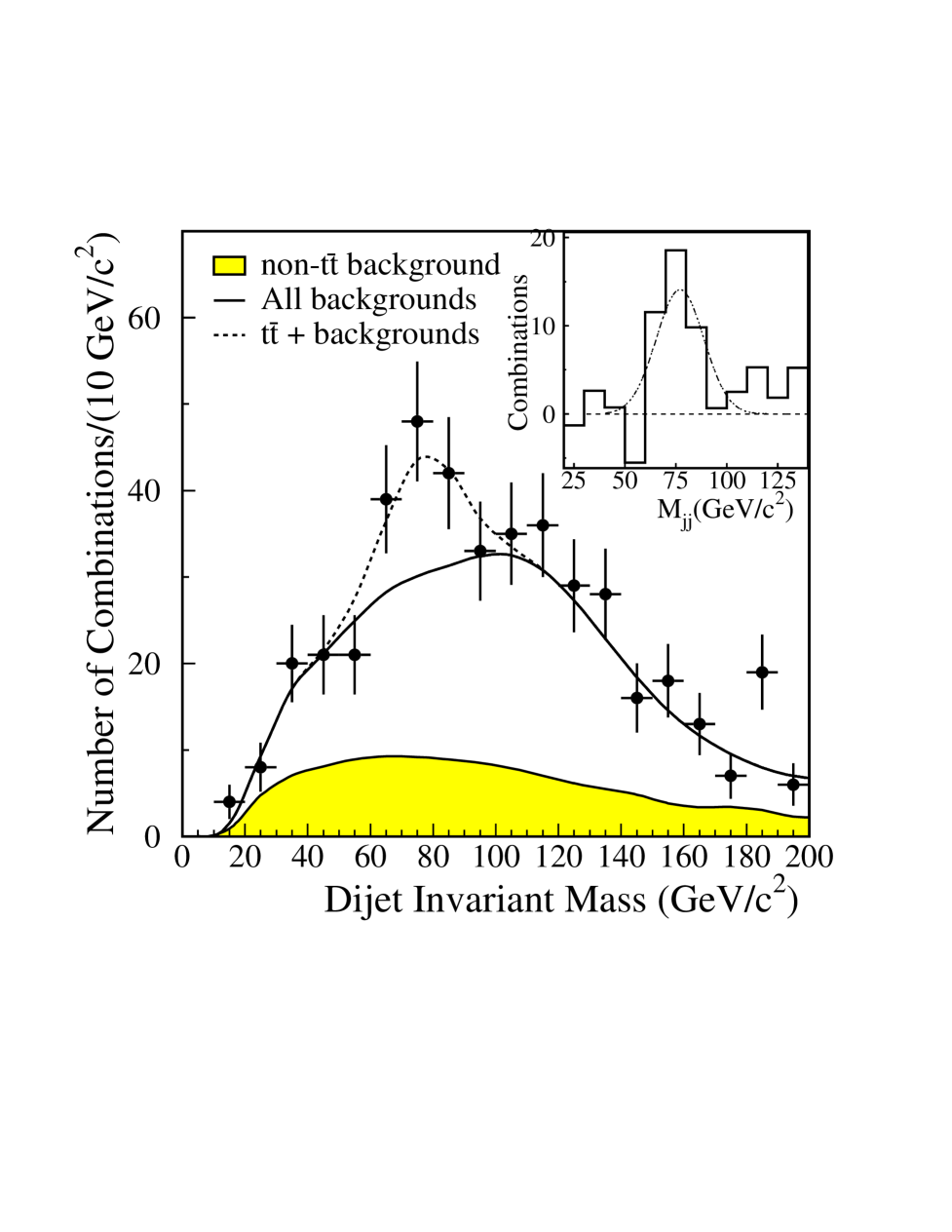
Fig. 56.: The dijet mass distribution from CDF data for $W+\geq 4~{}\text{jet}$ events after the cut $E_{T}^{\ell}+\sum E_{T}^{\text{jet}}>310~{}\text{GeV}$. The points are the data, the shaded curve is the vecbos $W+\text{jets}$ background, and the solid curve is the sum of that and the $t\overline{t}$ combinatorial background. The dotted curve is the result of a Gaussian fit to the $W$ boson mass peak. The inset plot shows the peak after background subtraction. From Ref. [cdfhadw97].

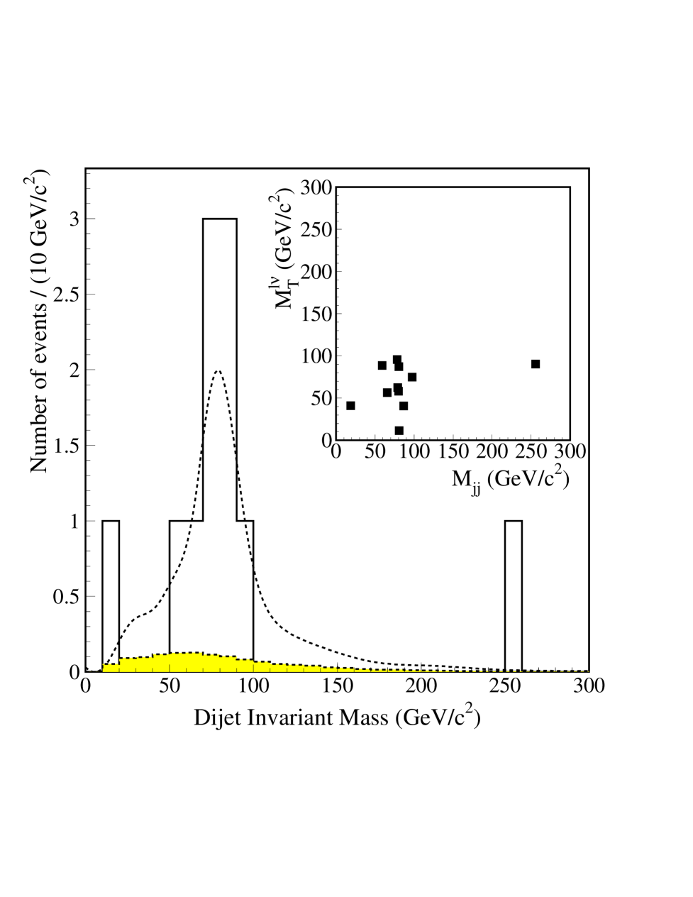
Fig. 57.: Dijet mass distribution of the two untagged jets in the CDF double $b$-tag sample. The shaded curve is the expected background contribution, and the dashed curve is the expectation for $t\overline{t}$ signal plus background. The inset compares the lepton-${\hbox{$E$\kern-6.00006pt\lower-0.43057pt\hbox{/}}}_{T}$ transverse mass to the dijet invariant mass for these eleven events. From Ref. [cdfhadw97].

8 Prospects for Run 2

8.1 Accelerator and Detector Upgrades

The Tevatron collider Run 1 ended in February, 1996. The accelerator and both detectors are presently undergoing major upgrades for the next run, due to start in the year 2000.

The major improvement to the accelerator complex will be the addition of the Main Injector. This $3319~{}\text{m}$ circumference machine is composed of conventional magnets and has a maximum energy of $150~{}\text{GeV}$ and a minimum cycle time of $\sim 1.5~{}\text{s}$. It will replace the Main Ring, and will serve as the injector into the Tevatron. It will also be used to produce antiprotons, thus removing the detector deadtimes incurred by running beam in the Main Ring during collider operations. (It can also be used to support fixed target experiments running concurrently with the collider.) The Main Injector is expected to increase the peak luminosity of the Tevatron from the present value of $\sim 2\times 10^{31}\,\text{cm}^{-2}\text{s}^{-1}$ to $\sim 8\times 10^{31}\,\text{cm}^{-2}\text{s}^{-1}$. A second machine, the Recycler, will be built in the same tunnel as the Main Injector.[recyclertdr] It will be constructed almost entirely from permanent magnets, and will operate at a fixed energy of $8~{}\text{GeV}$. Its principal function will be to serve as a high-reliability repository for antiprotons. It will also be used to capture unused antiprotons from the Tevatron at the end of a store, recool them, and use them again in another collider store. Use of the Recycler is expected to increase the peak luminosity to $\sim 2\times 10^{32}\,\text{cm}^{-2}\text{s}^{-1}$. In addition, the superconducting magnets of the Tevatron will be operated at a lower temperature; this should enable an increase of the center-of-mass energy from $\sqrt{s}=1.8~{}\text{TeV}$ to $\sqrt{s}\approx 2.0~{}\text{TeV}$. This corresponds to about a $40\%$ increase in the $t\overline{t}$ production cross section. The goal for the integrated luminosity in the next collider run is $2~{}\text{fb}^{-1}$ per experiment. Also envisioned is a possible Run 3, with additional improvements to the proton and antiproton sources, which could reach an integrated luminosity of $\sim 30~{}\text{fb}^{-1}$.

Both collider detectors will be upgraded[cdfupgrade] for Run 2. The DØ detector will acquire a central magnetic field, a silicon vertex detector, and a scintillating fiber tracker, while CDF will upgrade to an expanded vertex detector that will provide coverage of the entire luminous region of the beam. These improvements will significantly increase the efficiency for tagging $b$-jets in $t\overline{t}$ decays. Many other improvements will also be made to both detectors in outer tracking, calorimetry, and muon coverage.

8.2 Cross Section and Mass Measurements

CDF and DØ have made impressively precise measurements of the top quark mass: $m_{t}=175.3\pm 6.4~{}\text{GeV}/c^{2}$, and $m_{t}=172.1\pm 7.1~{}\text{GeV}/c^{2}$, respectively. The corresponding cross sections are $\sigma_{t\overline{t}}=7.6^{+1.8}_{-1.5}~{}\text{pb}$ and $5.6\pm 1.8~{}\text{pb}$. These results are based on samples that range in size from about five to one hundred events. In the next run, sample sizes should increase by at least twenty-fold.

The potential for $t\overline{t}$ physics at the Tevatron during Run 2 and beyond has been studied extensively.[tev2k, aspentop] The expected yields for each detector are on the order of 160 dilepton events, 1200 $\text{lepton}+\geq 4~{}\text{jets}$ events, and 500 double-tagged $\text{lepton}+\geq 4~{}\text{jets}$ events. For the cross section measurement, the statistical component of the uncertainty scales as $1/\sqrt{N}$. The dominant contributions to the systematic uncertainty are the uncertainties in the $t\overline{t}$ acceptance and background estimates. Both of these are amenable to study using control samples from the data, and therefore can be also expected to scale as $1/\sqrt{N}$. The limiting factor could be the error on the luminosity, which can be measured to $\sim 5\%$ using the $W\rightarrow\ell\nu$ rate. With these assumptions, the precision of the cross section measurement in Run 2 should be about $8$–$10\%$.

For the mass measurement, the statistical uncertainty should again scale as $1/\sqrt{N}$. However, the present measurements are already limited by systematic uncertainties, so the challenge will be to reduce this component. One of the dominant uncertainties is that in the jet energy scale. However, given large statistics, the energy scale can be well characterized using $Z+\text{multijet}$ events. With an adequate sample of double $b$-tagged events, it should be possible to use the hadronically-decaying $W$ bosons in $t\overline{t}\rightarrow\ell+\text{jets}$ channels to perform an in situ calibration of the energy scale. Therefore, the uncertainty on the jet scale should decrease as $1/\sqrt{N}$. The other major uncertainty is that in modeling QCD radiative effects in $t\overline{t}$ decays. Presently, these are modeled using parton-shower Monte Carlo programs such as herwig. However, some theoretical progress has recently been made in understanding the phenomenology of gluon radiation in $t\overline{t}$ events,[orr97, masuda96] and the situation should be greatly helped by the availability of $t\overline{t}$ data with sufficient statistics to provide meaningful constraints on models. We therefore expect this uncertainty also to decrease. The total achievable uncertainty in the top quark mass measurement from Run 2 should be about $3$–$4~{}\text{GeV}/c^{2}$ for each experiment.

A precise measurement of the top quark mass, along with that of the $W$ boson provides a crucial test of the electroweak theory as well as a strong constraint on the mass of the Higgs boson. Figure 58 shows the correlation between the W boson mass and top quark mass for a range of Higgs boson masses. Also plotted are the current direct and indirect measurements of $m_{t}$ and $M_{W}$.

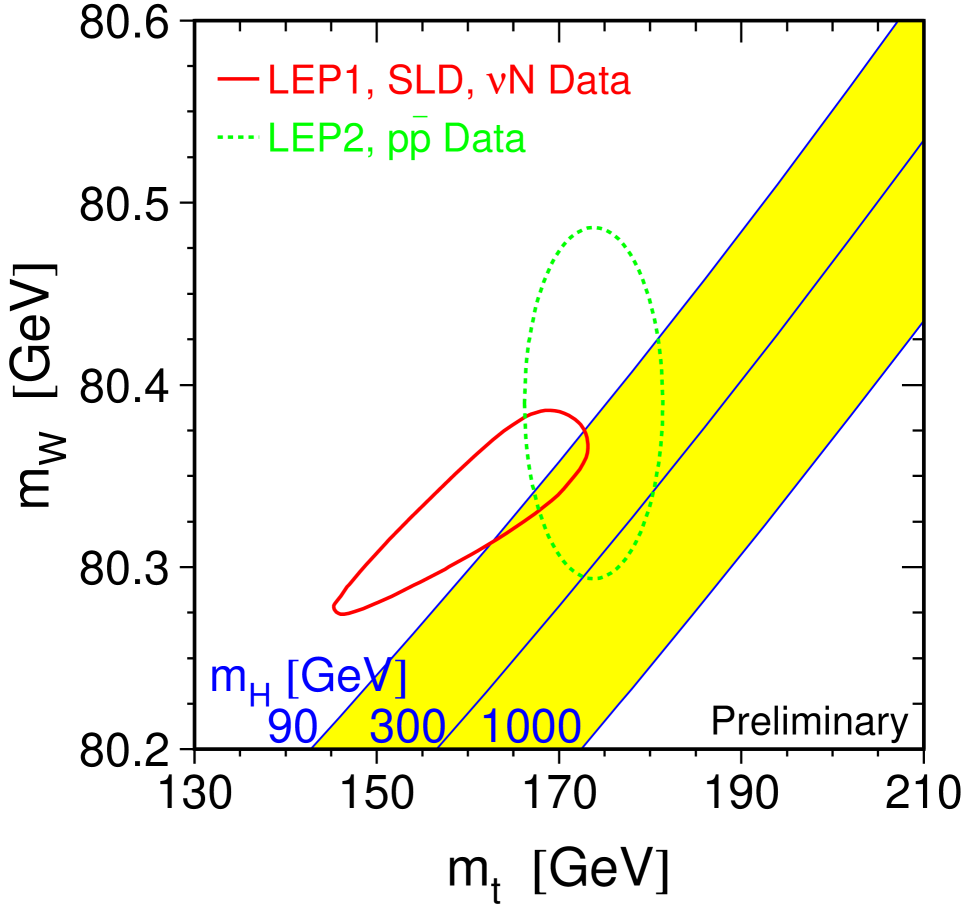
Fig. 58.: The correlation between the $W$ boson mass and the top quark mass as predicted by the electroweak theory of the Standard Model, for various possible masses of the yet undiscovered Higgs boson mass. From Ref.[lepewg98]. (Each line corresponds the mass value shown.) Also shown are the measured $W$ boson mass and the direct and indirect measurements of the top quark mass. As the errors in the measurements of $M_{W}$ and $m_{t}$ decrease, the Higgs boson mass can be better constrained.

8.3 Single Top Quark Production

So far, this review has focussed on the QCD pair production of top quarks. As mentioned in Sec. 2, top quarks can also be produced singly, through the electroweak “$W^{*}$” (Fig. 4) and $W$-gluon fusion (Fig. 5) processes.[heinson97b, heinson97a, tait97] (There is also a contribution from $p\overline{p}\rightarrow tW$, but the rate for that process is very small at the Tevatron.) The cross sections for these processes have been calculated at NLO. The results for $m_{t}=175~{}\text{GeV}/c^{2}$ and $\sqrt{s}=2~{}\text{TeV}$ are $\sigma(p\overline{p}\rightarrow t\overline{b}(\overline{t}b)+X)=0.9~{}\text{pb}$ for the $W^{*}$ process,[smith96] and $\sigma(p\overline{p}\rightarrow tq(\overline{t}\overline{q})+X)=2.4~{}\text{pb}$ for the $W$-gluon fusion process.[stelzer97] These should be compared to the resummed NLO $t\overline{t}$ cross section of $\sim 7~{}\text{pb}$.[bonciani98]

The single top quark production cross section is directly proportional to $|V_{tb}|^{2}$. Therefore, a measurement of the cross section gives a measurement of $|V_{tb}|$, independent of any assumptions about the unitarity of the CKM matrix. Note that this strict proportionality fails in the presence of certain forms of new physics, such as anomalous couplings of the top quark. However, evidence for such new physics should also be present in quantities which do not depend on $|V_{tb}|$, such as the ratio of the two subprocess cross sections,[heinson97b, tait97] so the effects can, in principle, be disentangled.

One would search for single top quark events by selecting events with exactly one high-$p_{T}$ lepton, large ${\hbox{$E$\kern-6.00006pt\lower-0.43057pt\hbox{/}}}_{T}$, and exactly two jets, one of which has a $b$-tag. This sort of selection would yield a signal/background ratio of about $1:2$,[tev2k] the dominant background being $Wb\overline{b}$ production, with smaller contributions from $t\overline{t}$ pair production and other QCD processes. The signal can be further enhanced by plotting the distribution of $m(Wb)$ and looking for an excess at around the known mass of the top quark, as shown in Fig. 59.

Fig. 59.: Reconstructed top quark invariant mass for single top quark signal and background, after typical selection cuts. For $\sqrt{s}=2.0~{}\text{TeV}$ and $m_{t}=170~{}\text{GeV}/c^{2}$. The vertical scale is normalized to a total integrated luminosity of $1~{}\text{fb}^{-1}$. From Ref.[tev2k].

In Run 2, with $2~{}\text{fb}^{-1}$, $|V_{tb}|$ can probably be measured to a precision of $\sim 10\%$.[tev2k] (The limiting factor in this measurement is expected to be the error on the total integrated luminosity, which has been assumed to be $5\%$.)

8.4 Top and New Physics

The large mass of the top quark is certainly allowed in the Standard Model, but is not required. In fact, the Standard Model offers no explanation as to why the top quark is so heavy. But because of its large mass, the top quark may be a sensitive probe of new physics. The heaviness of the top quark may, in fact, reflect the presence of new physics at the electroweak scale. Furthermore, as we discussed in Sec. 1, in supersymmetric theories, a heavy top quark can induce the spontaneous breakdown of electroweak symmetry. If this were found to be true, it would represent a major step forward in our understanding of the origin of mass. We mention below some popular theories of new physics, and outline the ways in which its manifestations might be studied using the top quark.

A very promising class of theories is based on the concept of supersymmetry. (See Ref. [dawson96] for a recent review.) There are many valid and intriguing reasons for the prevailing optimism concerning their veracity: supersymmetric theories permit the unification of the strong, weak, and electromagnetic coupling constants at a grand unification (GUT) scale, consistent with the experimental bound on the proton lifetime; they solve the problems of gauge hierarchy and naturalness. To add to their allure, superstring theories, which may lead to a theory of all forces, predict supersymmetry!

Supersymmetry (SUSY) is a conjectured symmetry between fermions and bosons that predicts the existence of a supersymmetric partner for each particle of the Standard Model. (SUSY can also be construed, in a more profound way, as an augmentation of spacetime with fermionic dimensions.) In some supersymmetric models, top quarks can be produced in the decay of heavy supersymmetric particles; the top quark itself may also decay into lighter superpartners. The study and precise measurement of top quark production rates can provide useful information about such nonstandard processes. It is expected that the production of single top quarks, proceeding through electroweak processes, will be particularly sensitive to new physics. Supersymmetric theories usually impose conservation of “$R$-parity,” which is a quantum number defined such that it has a value of $R=+1$ for normal particles and $R=-1$ for their SUSY partners. However, $R$-parity conservation is not required, and if it is not imposed, the rate of single top quark production $q\overline{q}\rightarrow b\,\overline{t}$ can be greatly enhanced over that predicted by the Standard Model. Such reactions would be induced by the exchange of a supersymmetric quark (a “squark”) in the $t$-channel, which violates baryon number, as well as by the lepton-number violating exchange of a supersymmetric lepton (“slepton”) in the $s$-channel. The decay of a top quark into its supersymmetric partner (called a top squark or a “stop”) and the lightest neutralino, a process predicted in $R$-parity violating SUSY models, could be observed during the next run of the upgraded Tevatron.

Another attractive, perhaps radical, approach to understanding electroweak symmetry breaking and the origin of fermion masses and mixings, is that of new strong dynamics. In these theories, new strong interactions of fermions and bosons are invoked at the scale $\Lambda\sim 1~{}\text{TeV}$, and cause the dynamical breaking of electroweak symmetry. Consequently, no elementary scalar bosons (such as the Higgs) need exist. The popular models of new strong dynamics are those of technicolor, topcolor, and their variants. In the technicolor model,[weinberg76] which is analogous to QCD, the chiral symmetry is spontaneously broken through a technifermion condensation mechanism, thereby giving masses to the gauge bosons. The fermions acquire masses through new interactions (extended technicolor) with the technifermion condensate. To account for the heaviness of the top quark, one postulates the existence of new topcolor interactions.[topcolor] In these models, many signatures would involve the top quark in the final state. Particularly interesting and unique are signatures of resonances that decay to $t\overline{t}$. In technicolor models,[eichten_lane] a spin-zero color-octet resonance, the techni-eta, is produced in gluon-gluon collisions and decays into $t\overline{t}$ or a gluon pair. Such a resonance would be seen as a distortion or broadening of the $t\overline{t}$ or two-jet invariant mass distributions, but its effect on the $b\overline{b}$ mass distribution would be negligible. In topcolor models,[hill_parke] a spin-one coloron (top-gluon), produced mainly by quark-antiquark annihilations, would decay into $t\overline{t}$ and $b\overline{b}$ with roughly equal probability, and would appear as a broad resonance in both distributions. If an enhancement were to be observed in the $t\overline{t}$ mass spectrum, it would be important to study it at the Large Hadron Collider (LHC),[LHC] due for completion in 2005, at CERN. This machine will provide $pp$ collisions with a center-of-mass energy of $\sqrt{s}=14~{}\text{TeV}$, with luminosities of up to $10^{34}\ \text{cm}^{-2}\,\text{s}^{-1}$. At the LHC, 90% of the top quark pairs are expected to be produced by gluon-gluon fusion, in contrast with the Tevatron, where 90% of the top quark pairs come from quark-antiquark annihilations. The aforementioned models have very different predictions of rates and consequences at the two colliders. The two colliders hold promise of great discoveries and perhaps some surprises.

Finally, as Chris Quigg has noted recently,[quigg97b] in spite of its fleeting existence, the top quark may, in fact, have a profound effect on the basic properties of the everyday world. At the dawn of the third millennium, with the improved Tevatron and upgraded CDF and DØ detectors, we expect to refine the measurements of the properties of the top quark and to study its dynamics, not only for its own sake, but also in the hope that we shall be afforded the good fortune to unravel some of nature’s mysteries.

REFERENCES

- [1]
- [2] CDF Collaboration, F. Abe et al., Phys. Rev. Lett. 74, 2626 (1995).
- [3] CDF Collaboration, F. Abe et al., Phys. Rev. D50, 2966 (1994).
- [4] DØ Collaboration, S. Abachi et al., Phys. Rev. Lett. 74, 2632 (1995).
- [5] S. Weinberg, Phys. Rev. Lett. 19, 1264 (1967); A. Salam, Elementary Particle Physics (Almquvist and Wiksells, Stockholm, 1968); S. Glashow, J.Iliopoulos, and L. Maiani, Phys. Rev. D2, 1285 (1970); D. Gross and F. Wilczek, Phys. Rev. D8, 3633 (1973); ibid, Phys. Rev. Lett. 30, 1343 (1973); H. D. Politzer, Phys. Rev. Lett. 30, 1346 (1973); LEP Electroweak Working Group, Report No. CERN-PPE/96-183 (1996).
- [6] S. J. Wimpenny and B. L. Winer, Annu. Rev. Nucl. Part. Sci. 46, 149 (1996); C. Campagnari and M. Franklin, Rev. Mod. Phys. 69, 137 (1997).
- [7] R. M. Barnett et al., Phys. Rev. D54, 1 (1996), with updates from the 1997 WWW edition at http://www.lbl.gov/.
- [8] J. Ellis, Int. J. Mod. Phys. A12, 5531 (1997); G. Altarelli, R. Barbieri, and F. Caravaglios, Int. J. Mod. Phys. A13, 1031 (1998).
- [9] F. Wilczek, Int. J. Mod. Phys. A13, 863 (1998).
- [10] G. L. Kane and M. E. Peskin, Nucl. Phys. B195, 29 (1982); CLEO Collaboration, A. Bean et al., Phys. Rev. D35, 3533 (1987).
- [11] D. P. Roy and S. U. Sankar, Phys. Lett. B243, 296 (1990).
- [12] ARGUS Collaboration, H. Albrecht et al., Phys. Lett. B192, 245 (1987); ibid, Phys. Lett. B324, 249 (1994); CLEO Collaboration, J. Bartelt et al., Phys. Rev. Lett. 71, 1680 (1993).
- [13] C. Quigg, Gauge Theories of the Strong, Weak, and Electromagnetic Interactions (Benjamin/Cummings, Reading, MA, 1990).
- [14] PLUTO Collaboration, Ch. Berger et al., Phys. Lett. B76, 243 (1978); J. K. Bienlein et al., Phys. Lett. B78, 360 (1978); C. W. Darden et al., Phys. Lett. B76, 246 (1978).
- [15] LEP Collaborations, LEP Electroweak Group, and SLD Heavy Flavour Group, Report No. CERN-PPE/97-154 (1997).
- [16] D. Schaile and P. M. Zerwas, Phys. Rev. D45, 3262 (1992).
- [17] M. S. Chanowitz, M. A. Furman, and I. Hinchliffe, Phys. Lett. B78, 285 (1978); ibid, Nucl. Phys. B153, 402 (1979).
- [18] E. Eichten, I. Hinchliffe, K. Lane, and C. Quigg, Rev. Mod. Phys. 56, 579 (1984).
- [19] M. Martinez, R. Miquel, L. Rolandi, and R. Tenchini, Report No. CERN-EP/98-027 (1998).
- [20] E. H. Simmons, in Beyond the Standard Model V, Balholm, Norway (AIP, Woodbury, NY, 1997); L. Ibáñez, Nucl. Phys. B218, 514 (1983); L. Alvarez-Gaumé, J. Polchinski, and M. B. Wise, Nucl. Phys. B221, 495 (1983).
- [21] UA1 Collaboration, C. Albajar et al., Z. Phys. C48, 1 (1990); UA2 Collaboration, T. Åkesson et al., Z. Phys. C46, 179 (1990).
- [22] M. Cacciari, in Symposium on Twenty Beautiful Years of Bottom Physics - b20 (AIP, Woodbury, NY, 1998).
- [23] S. Frixione, M. L. Mangano, P. Nason, and G. Ridolfi, in Heavy Flavors II, edited by A. J. Buras and M. Linder (World Scientific, River Edge, NJ, 1997).
- [24] J. C. Collins, D. E. Soper, and G. Sterman, Nucl. Phys. B263, 37 (1986).
- [25] H. M. Georgi, S. L. Glashow, M. E. Machacek, and D. V. Nanopoulos, Ann. Phys. 114, 273 (1978); L. M. Jones and H. W. Wyld, Phys. Rev. D17, 1782 (1978); M. Glück, J. F. Owens, and E. Reya, Phys. Rev. D17, 2324 (1978); J. Babcock, D. Sivers, and S. Wolfram, Phys. Rev. D18, 162 (1978); K. Hagiwara and T. Yoshino, Phys. Lett. B80, 282 (1979); B. L. Combridge, Nucl. Phys. B151, 429 (1979).
- [26] P. Nason, S. Dawson, and R. K. Ellis, Nucl. Phys. B303, 607 (1988); ibid, Nucl. Phys. B327, 49 (1989); W. Beenakker, H. Kuijf, W. L. van Neerven, and J. Smith, Phys. Rev. D40, 54 (1989); W. Beenakker et al., Nucl. Phys. B351, 507 (1991); M. L. Mangano, P. Nason, and G. Ridolfi, Nucl. Phys. B373, 295 (1992); G. Altarelli, M. Diemoz, G. Martinelli, and P. Nason, Nucl. Phys. B308, 724 (1988); R. K. Ellis, Phys. Lett. B259, 492 (1991).
- [27] E. Laenen, J. Smith, and W. L. van Neerven, Phys. Lett. B321, 254 (1994); ibid, Nucl. Phys. B369, 543 (1992); N. Kidonakis and J. Smith, Phys. Rev. D51, 6092 (1995).
- [28] E. L. Berger and H. Contopanagos, Phys. Lett. B361, 115 (1995).
- [29] E. L. Berger and H. Contopanagos, Phys. Rev. D54, 3085 (1996); ibid, in Deep Inelastic Scattering and QCD: 5th International Workshop, Chicago, Il (AIP, Woodbury, NY, 1997).
- [30] E. L. Berger and H. Contopanagos, Phys. Rev. D57, 253 (1998).
- [31] H. Contopanagos and G. Sterman, Nucl. Phys. B400, 211 (1993); ibid, Nucl. Phys. B419, 77 (1994).
- [32] S. Catani, M. L. Mangano, P. Nason, and L. Trentadue, Phys. Lett. B378, 329 (1996).
- [33] R. Bonciani, S. Catani, M. L. Mangano, and P. Nason, Report No. CERN-TH/98-31 (1998), hep-ph/9801375.
- [34] A. D. Martin, R. G. Roberts, and W. J. Stirling, Phys. Lett. B387, 419 (1996).
- [35] A. D. Martin, W. J. Stirling, and R. G. Roberts, Phys. Lett. B306, 145 (1993).
- [36] H. L. Lai et al., Phys. Rev. D51, 4763 (1995).
- [37] A. P. Heinson, A. S. Belyaev, and E. E. Boos, Phys. Rev. D56, 3114 (1997).
- [38] W. Hollik, W. M. Mösle, and D. Wackeroth, Nucl. Phys. B516, 29 (1998); B. Lampe, Phys. Lett. B415, 63 (1997); S. Moretti, J. Phys. G24, 525 (1998).
- [39] L. H. Orr, Phys. Rev. D44, 88 (1991); I. Bigi, Y. Dokshitzer, V. Khoze, and P. Zerwas, Phys. Lett. B181, 157 (1986).
- [40] G. Marchesini et al., Comp. Phys. Comm. 67, 465 (1992).
- [41] G. Altarelli and G. Parisi, Nucl. Phys. B126, 298 (1977).
- [42] S. Frixione, M. L. Mangano, P. Nason, and G. Ridolfi, Phys. Lett. B351, 555 (1995).
- [43] L. H. Orr, T. Stelzer, and W. J. Stirling, Phys. Rev. D56, 446 (1997).
- [44] S. Mrenna and C.-P. Yuan, Phys. Rev. D55, 120 (1997).
- [45] T. Sjöstrand, Comp. Phys. Comm. 82, 74 (1994).
- [46] H. T. Edwards, Annu. Rev. Nucl. Part. Sci. 35, 605 (1985); Design Report Tevatron 1 Project, 1984, Fermilab internal note (unpublished).
- [47] W. J. Thompson, Ph.D. thesis, State University of New York at Stony Brook, Stony Brook, New York, 1994.
- [48] M. P. Church and J. P. Marriner, Annu. Rev. Nucl. Part. Sci. 43, 253 (1993).
- [49] D. Möhl, G. Petrucci, L. Thorndahl, and S. van der Meer, Phys. Rep. 58, 73 (1980).
- [50] CDF Collaboration, F. Abe et al., Nucl. Instrum. Methods Phys. Res., Sect. A271, 387 (1988); D. Amidei et al., Nucl. Instrum. Methods Phys. Res., Sect. A350, 73 (1994).
- [51] J. Antos et al., Nucl. Instrum. Methods Phys. Res., Sect. A360, 118 (1995).
- [52] DØ Collaboration, S. Abachi et al., Nucl. Instrum. Methods Phys. Res., Sect. A338, 185 (1994).
- [53] DØ Collaboration, S. Abachi et al., Phys. Rev. D52, 4877 (1995).
- [54] DØ Collaboration, B. Abbott et al., Phys. Rev. D58, 052001 (1998).
- [55] J. E. Huth et al., in Research directions for the decade: Snowmass ’90: proceedings, edited by E. L. Berger (World Scientific, River Edge, NJ, 1990), pp. 134–136.
- [56] CDF Collaboration, F. Abe et al., Phys. Rev. D47, 4857 (1993); DØ Collaboration, R. Kehoe, in Frascati 1996, Calorimetetry in High Energy Physics (World Scientific, River Edge, NJ, 1996), pp. 349–358; DØ Collaboration, B. Abbott et al., Report No. Fermilab-Pub-97/330-E (1998), hep-ex/9805009, submitted to Nucl. Instrum. Methods.
- [57] DØ Collaboration, B. Abbott et al., Report No. Fermilab-Pub-97/422-E (1997), hep-ex/9712029, submitted to Phys. Rev. D.
- [58] DØ Collaboration, S. Abachi et al., Nucl. Instrum. Methods Phys. Res., Sect. A324, 53 (1993); DØ Collaboration, H. Aihara et al., Nucl. Instrum. Methods Phys. Res., Sect. A325, 393 (1993).
- [59] CDF Collaboration, F. Abe et al., Phys. Rev. Lett. 79, 3585 (1997).
- [60] CDF Collaboration, F. Abe et al., Phys. Rev. Lett. 80, 2773 (1998).
- [61] CDF Collaboration, F. Abe et al., Phys. Rev. D57, 5382 (1998).
- [62] DØ Collaboration, S. Abachi et al., Phys. Rev. Lett. 79, 1203 (1997).
- [63] V. Barger, J. Ohnemus, and R. J. N. Phillips, Phys. Rev. D48, 3953 (1993).
- [64] H. Baer, V. Barger, and R. J. N. Phillips, Phys. Rev. D39, 3310 (1989); A. K. Likhoded and S. R. Slabospitskii, Yad. Fiz. 52, 1106 (1990).
- [65] S. W. Herb et al., Phys. Rev. Lett. 39, 252 (1977).
- [66] CELLO Collaboration, H.-J. Behrend et al., Phys. Lett. B144, 297 (1984); JADE Collaboration, W. Bartel et al., Phys. Lett. B88, 171 (1979); ibid, Phys. Lett. B89, 136 (1979); ibid, Phys. Lett. B99, 277 (1981); MARK-J Collaboration, D. P. Barber et al., Phys. Lett. B85, 463 (1979); ibid, Phys. Rev. Lett. 44, 1722 (1980); MARK-J Collaboration, B. Adeva et al., Phys. Rev. Lett. 50, 799 (1983); ibid, Phys. Rev. Lett. 51, 443 (1983); ibid, Phys. Lett. B152, 439 (1985); ibid, Phys. Rev. D34, 681 (1986); PLUTO Collaboration, C. Berger et al., Phys. Lett. B86, 413 (1979); TASSO Collaboration, R. Brandelik et al., Phys. Lett. B113, 499 (1982); TASSO Collaboration, M. Althoff et al., Z. Phys. C22, 307 (1984); ibid, Phys. Lett. B138, 441 (1984).
- [67] AMY Collaboration, H. Sagawa et al., Phys. Rev. Lett. 60, 93 (1988); AMY Collaboration, S. Igarashi et al., Phys. Rev. Lett. 60, 2359 (1988); TOPAZ Collaboration, I. Adachi et al., Phys. Rev. Lett. 60, 97 (1988); VENUS Collaboration, H. Yoshida et al., Phys. Lett. B198, 570 (1987); VENUS Collaboration, K. Abe et al., Phys. Lett. B234, 382 (1990).
- [68] MARK II Collaboration, G. S. Abrams et al., Phys. Rev. Lett. 63, 2447 (1989).
- [69] ALEPH Collaboration, D. Decamp et al., Phys. Lett. B236, 511 (1990); DELPHI Collaboration, P. Abreu et al., Phys. Lett. B242, 536 (1990); OPAL Collaboration, M. Z. Akrawy et al., Phys. Lett. B236, 364 (1990).
- [70] CERN ISR Division, Report No. CERN/ISR-DI/82-02 (1982).
- [71] UA1 Collaboration, G. Arnison et al., Phys. Lett. B147, 493 (1984).
- [72] UA1 Collaboration, C. Albajar et al., Z. Phys. C37, 505 (1988).
- [73] CDF Collaboration, F. Abe et al., Phys. Rev. Lett. 64, 142 (1990); ibid, Phys. Rev. Lett. 64, 147 (1990); ibid, Phys. Rev. D43, 664 (1991).
- [74] CDF Collaboration, F. Abe et al., Phys. Rev. Lett. 68, 447 (1992); ibid, Phys. Rev. D45, 3921 (1992).
- [75] DØ Collaboration, S. Abachi et al., Phys. Rev. Lett. 72, 2138 (1994).
- [76] CDF Collaboration, F. Abe et al., Phys. Rev. Lett. 73, 225 (1994).
- [77] DØ Collaboration, S. Abachi et al., Phys. Rev. Lett. 74, 2422 (1995).
- [78] CDF Collaboration, S.-B. Kim, in Physics in Collision 15: Proceedings (World Scientific, River Edge, NJ, 1996), pp. 1–26.
- [79] DØ Collaboration, P. C. Bhat, in Proceedings of the 8th Meeting of the Division of Particles and Fields of the American Physical Society, Albuquerque, New Mexico, USA (World Scientific, River Edge, NJ, 1994), p. 705.
- [80] F. Paige and S. Protopopescu, BNL Report 38034, Brookhaven, 1986 (unpublished).
- [81] F. A. Berends, H. Kuijf, B. Tausk, and W. T. Giele, Nucl. Phys. B357, 32 (1991).
- [82] CDF Collaboration, F. Abe et al., Phys. Rev. Lett. 80, 2779 (1998).
- [83] CDF Collaboration, F. Abe et al., Phys. Rev. Lett. 79, 1992 (1997).
- [84] R. Decker et al., Comp. Phys. Comm. 76, 361 (1993).
- [85] CDF Collaboration, D. W. Gerdes, in Proceedings of the 32nd Rencontres de Moriond: Electroweak Interactions and Unified Theories, Les Arcs, France (Editions Frontieres, Gif-sur-Yvette, France, 1997), pp. 69–76.
- [86] DØ Collaboration, P. C. Bhat, in 10th Topical Workshop on Proton-Antiproton Collider Physics: Batavia, Il (AIP, Woodbury, NY, 1995), p. 308.
- [87] DØ Collaboration, H. Prosper et al., in Proceedings of the International Conference on Computing in High Energy Physics ’95, Rio de Janeiro, Brazil (World Scientific, River Edge, NJ, 1996).
- [88] DØ Collaboration, N. Amos, in Proceedings of the 33rd Rencontres de Moriond, QCD and High Energy Hadronic Interactions (Editions Frontieres, Gif-sur-Yvette, France, 1998).
- [89] DØ Collaboration, B. Klima, in Results and Perspectives in Particle Physics, La Thuile, Italy (Editions Frontieres, Gif-sur-Yvette, France, 1998), hep-ex/9804017, Fermilab-Conf-98/137-E.
- [90] DØ Collaboration, B. Abbott et al., Report No. Fermilab-Pub-98/130-E (1998), hep-ex/9808034, submitted to Phys. Rev. D.
- [91] F. Tkachov, Int. J. Mod. Phys. A12, 5411 (1997).
- [92] W. T. Giele and E. W. N. Glover, Report No. Fermilab-Pub-97/413-T (1997), submitted to Phys. Rev. Lett.
- [93] F. James, Comp. Phys. Comm. 20, 29 (1980).
- [94] H. B. Prosper, Phys. Lett. B335, 515 (1994).
- [95] R. Roser, private communication; CDF Collaboration, W. Yao, in Proceedings of the XXIX International Conference on High Energy Physics, Vancouver, Canada (World Scientific, River Edge, NJ, 1998).
- [96] CDF Collaboration, F. Abe et al., Phys. Rev. Lett. 80, 2767 (1998).
- [97] DØ Collaboration, S. Abachi et al., Phys. Lett. B357, 500 (1995).
- [98] F. James, Rep. Prog. Phys. 43, 1145 (1980).
- [99] K. Kondo, J. Phys. Soc. Japan 57, 4126 (1988); ibid, J. Phys. Soc. Japan 60, 836 (1991); ibid, J. Phys. Soc. Japan 62, 1177 (1993).
- [100] R. H. Dalitz and G. R. Goldstein, Phys. Rev. D45, 1531 (1992); ibid, Phys. Lett. B287, 225 (1992).
- [101] DØ Collaboration, B. Abbott et al., Phys. Rev. Lett. 80, 2063 (1998).
- [102] DØ Collaboration, B. Abbott et al., Report No. Fermilab-Pub-98/261-E (1998), hep-ex/9808029, submitted to Phys. Rev. D.
- [103] G. D’Agostini, Report No. DESY-95-242 (1995).
- [104] L. Holmström, S. R. Sain, and H. E. Miettinen, Comp. Phys. Comm. 88, 195 (1995).
- [105] DØ Collaboration, S. Abachi et al., Phys. Rev. Lett. 79, 1197 (1997).
- [106] DØ Collaboration, M. Strovink, in Proceedings of the XI Symposium on Hadron Collider Physics, Padua, Italy (World Scientific, River Edge, NJ, 1996), Fermilab-Conf-96/336-E.
- [107] P. C. Bhat, H. B. Prosper, and S. Snyder, Phys. Lett. B407, 73 (1997).
- [108] B. Klima, private communication.
- [109] N. Cabibbo, Phys. Rev. Lett. 10, 531 (1963); M. Kobayashi and T. Maskawa, Prog. Theor. Phys. 49, 652 (1973).
- [110] CDF Collaboration, G. F. Tartarelli, in Proceedings of International Europhysics Conference on High-Energy Physics (HEP 97), Jerusalem, Israel (World Scientific, River Edge, NJ, 1997), Fermilab-Conf-97/401-E.
- [111] A. P. Heinson, in Honolulu 1997, Physics and CP Violation (World Scientific, River Edge, NJ, 1997), pp. 369–376, Fermilab-Conf-97/238-E, hep-ex/9707026.
- [112] The TeV-2000 Group Report, 1996, Fermilab-Pub-96/082.
- [113] J. Swain and L. Taylor, Report No. hep-ph/9712420 (1997).
- [114] S. L. Glashow, J. Iliopoulos, and L. Maiani, Phys. Rev. D2, 1285 (1970).
- [115] G. Eilam, J. L. Hewett, and A. Soni, Phys. Rev. D44, 1473 (1991); B. Mele, S. Petrarca, and A. Soddu, Phys. Lett. B435, 401 (1998).
- [116] H. Fritzsch, Phys. Lett. B224, 423 (1989); D. Atwood, L. Reina, and A. Soni, Phys. Rev. D53, 1199 (1996); M. Luke and M. J. Savage, Phys. Lett. B307, 387 (1993); J. L. Diaz-Cruz and G. L. Castro, Phys. Lett. B301, 405 (1993); B. Grzadkowski, J. F. Gunion, and P. Krawczyk, Phys. Lett. B268, 106 (1991).
- [117] K. Agashe and M. Graesser, Phys. Rev. D54, 4445 (1995); J. M. Yang and C. S. Li, Phys. Rev. D49, 3412 (1994); C. S. Li, R. J. Oakes, and J. M. Yang, Phys. Rev. D49, 293 (1994).
- [118] A. Datta, J. M. Yang, B.-L. Young, and X. Zhang, Phys. Rev. D56, 3107 (1997).
- [119] W. Buchmüller and M. Gronau, Phys. Lett. B220, 641 (1989).
- [120] T. Han, K. Whisnant, B.-L. Young, and X. Zhang, Phys. Rev. D55, 7241 (1997); T. Han, R. Peccei, and X. Zhang, Nucl. Phys. B454, 527 (1995).
- [121] CDF Collaboration, F. Abe et al., Phys. Rev. Lett. 80, 2525 (1998).
- [122] J. F. Gunion, H. E. Haber, G. Kane, and S. Dawson, The Higgs Hunter’s Guide (Addison-Wesley, New York, 1990).
- [123] E. Ma, D. P. Roy, and J. Wudka, Phys. Rev. Lett. 80, 1162 (1998).
- [124] CDF Collaboration, B. Bevensee, in Proceedings of the 33rd Rencontres de Moriond, QCD and High Energy Hadronic Interactions (Editions Frontieres, Gif-sur-Yvette, France, 1998), Fermilab-Conf-98/155-E.
- [125] V. Barger, J. L. Hewett, and R. J. N. Phillips, Phys. Rev. D41, 3421 (1990).
- [126] DELPHI Collaboration, P. Abreu et al., Phys. Lett. B420, 140 (1998); OPAL Collaboration, K. Ackerstaff et al., Phys. Lett. B426, 180 (1998); ALEPH Collaboration, R. Barate et al., Phys. Lett. B418, 419 (1998).
- [127] OPAL Collaboration, G. Alexander et al., Phys. Lett. B370, 174 (1996); DELPHI Collaboration, P. Abreu et al., Z. Phys. C64, 183 (1994); L3 Collaboration, O. Adriani et al., Phys. Lett. B294, 457 (1992); ALEPH Collaboration, D. Decamp et al., Phys. Rep. 216, 253 (1992).
- [128] S. de Jong, Higgs searches at LEP, talk at 1998 Rencontres de Moriond.
- [129] UA1 Collaboration, C. Albajar et al., Phys. Lett. B257, 459 (1991); UA2 Collaboration, J. Alitti et al., Phys. Lett. B280, 137 (1992).
- [130] CDF Collaboration, F. Abe et al., Phys. Rev. D54, 735 (1996); ibid, Phys. Rev. Lett. 73, 2667 (1994).
- [131] M. Guchait and D. P. Roy, Phys. Rev. D55, 7263 (1997).
- [132] A. Stahl and H. Voss, Z. Phys. C74, 73 (1997).
- [133] CLEO Collaboration, M. S. Alam et al., Phys. Rev. Lett. 74, 2885 (1995).
- [134] T. Goto and Y. Okada, Prog. Theor. Phys. Suppl. 123, 213 (1996).
- [135] CDF Collaboration, F. Abe et al., Phys. Rev. Lett. 79, 357 (1997).
- [136] CDF Collaboration, S. Leone, Nucl. Phys. Proc. Suppl. 64, 406 (1998).
- [137] CDF Collaboration, F. Abe et al., Phys. Rev. Lett. 80, 5720 (1998).
- [138] ALEPH Collaboration, D. Buskulic et al., Phys. Lett. B313, 535 (1993).
- [139] G. Jackson et al., Fermilab-TM-1991, Fermilab, 1996 (unpublished).
- [140] CDF Collaboration, C. Newman-Holmes, Report No. Fermilab-Conf-96/218-E (1996); CDF Collaboration, R. Blair et al., Report No. Fermilab-Conf-96/390-E (1996); DØ Collaboration, S. Abachi et al., Report No. Fermilab-Pub-96/357-E (1996).
- [141] R. Frey et al., Report No. Fermilab-Conf-97/085 (1997), hep-ph/9704243.
- [142] B. Masuda, L. H. Orr, and W. J. Stirling, Phys. Rev. D54, 4453 (1996).
- [143] LEP Collaborations, LEP Electroweak Group, and SLD Heavy Flavour Group, 1998, http://www.cern.ch/LEPEWWG/plots/summer98.
- [144] T. Tait and C.-P. Yuan, Report No. MSUHEP-71015, hep-ph/9710372 (1997).
- [145] M. C. Smith and S. Willenbrock, Phys. Rev. D54, 6696 (1996).
- [146] T. Stelzer, Z. Sullivan, and S. Willenbrock, Phys. Rev. D56, 5919 (1997).
- [147] S. Dawson, in Techniques and Concepts of High-Energy Physics IX, edited by T. Ferbel (Plenum Press, New York, 1997), hep-ph/9612229.
- [148] S. Weinberg, Phys. Rev. D13, 974 (1976); L. Susskind, Phys. Rev. D20, 2619 (1979); E. Farhi and L. Susskind, Phys. Rep. 74, 277 (1981); S. F. King, Rep. Prog. Phys. 58, 263 (1995).
- [149] C. Hill, Phys. Lett. B345, 483 (1995).
- [150] E. Eichten and K. Lane, Phys. Lett. B327, 129 (1994).
- [151] C. Hill and S. Parke, Phys. Rev. D49, 4454 (1994).
- [152] See for example J. P. Gourber, Report No. CERN-LHC-Project-Report-167 (1998).
- [153] C. Quigg, Physics Today 50, 20 (1997), (No. 5).