Measurement of the top quark pair production cross section in
$p\bar{p}$ collisions using multijet final states

Abstract

We have studied $t\bar{t}$ production using multijet final states in $p\bar{p}$ collisions at a center-of-mass energy of 1.8 TeV, with an integrated luminosity of 110.3 pb^-1. Each of the top quarks with these final states decays exclusively to a bottom quark and a $W$ boson, with the $W$ bosons decaying into quark-antiquark pairs. The analysis has been optimized using neural networks to achieve the smallest expected fractional uncertainty on the $t\bar{t}$ production cross section, and yields a cross section of 7.1 $\pm$ 2.8 (stat) $\pm$ 1.5 (syst) pb, assuming a top quark mass of 172.1 GeV/$c^{2}$. Combining this result with previous DØ measurements, where one or both of the $W$ bosons decay leptonically, gives a $t\bar{t}$ production cross section of 5.9 $\pm$ 1.2 (stat) $\pm$ 1.1 (syst) pb.

Contents

toc

I Introduction

In the standard model, the top quark decays to a $b$ quark and a $W$ boson, and the dominant decay of the $W$ boson is into a quark-antiquark pair. Events with a $t\bar{t}$ pair can have both $W$ bosons decaying to quarks. This is referred to as the “all-jets” channel, and is expected to account for 44% of the $t\bar{t}$ production cross section.

The observation of top quark production [3, 4] in the channels involving one or two leptons motivates us to investigate $t\bar{t}$ decays into other channels. DØ has measured a top quark mass, $m_{t}$, of 172.1 $\pm$ 5.2 (stat) $\pm$ 4.9 (syst) GeV/$c^{2}$ [5] and a $t\bar{t}$ production cross section of 5.6 $\pm$ 1.4 (stat) $\pm$ 1.2 (syst) pb [6], while CDF has measured a mass of 175.9 $\pm$ 4.8 (stat) $\pm$ 4.9 (syst) GeV/$c^{2}$ [7] and a $t\bar{t}$ production cross section of 7.6 ${}^{+1.8}_{-1.5}$ pb [8]. Recently, CDF has reported on the all-jets channel [9], and finds the $t\bar{t}$ production cross section to be 10.1 ${}^{+4.5}_{-3.6}$ pb and a top quark mass of 186 $\pm$ 10 (stat) $\pm$ 12 (syst) GeV/$c^{2}$.

The work presented here is based on 110.3 $\pm$ 5.8 pb^-1 of data recorded between August 1992 and February 1996 at the Fermilab Tevatron collider, with a $p\bar{p}$ center-of-mass energy of 1.8 TeV. Assuming the branching ratio and cross section predicted by the standard model, we expect approximately 200 $t\bar{t}\rightarrow$ all-jets events in this data sample.

The signature for $t\bar{t}$ production in the all-jets channel is six or more high transverse momentum jets with kinematic properties consistent with the top quark decay hypothesis. At least two of these jets originate from $b$ quarks. The background to this signature consists of events from other processes that can also produce six or more jets. The $t\bar{t}$ channel is one of the few examples of multijet final states that are dominated by quarks rather than gluons. This fact has motivated us to include the characteristic differences between quark and gluon jets in separating the top quark to all-jets signal from background.

Interest in the all-jets decay channel of top quarks also stems from the fact that, without any unobserved particles in the final-state, the all-jets mode is the most kinematically constrained of all the top quark decay channels. Furthermore, since the top quark is quite massive, decays via charged Higgs may be possible. If channels such as $t\rightarrow H^{+}b$ have a significant branching fraction, the main effect could be a deficit in the $t\bar{t}$ final states with energetic electrons or muons, relative to the all-jets channel.

II Outline of Method

The search for the top quark in the all-jets channel began with the imposition of preliminary selection criteria at the trigger stage, followed by more stringent criteria in the offline analysis. As these initial criteria were not very restrictive, the observed cross section, primarily from QCD processes, was more than three thousand times larger than the expected signal. The principal challenge in the search was to develop a set of selection criteria that could significantly improve the signal-to-background ratio, and provide an estimate of the background remaining after imposing any selection requirements.

The data sample consisted of over 600,000 events after the initial selection criteria. Because of the small number of $t\bar{t}$ events expected in the presence of this large background, and with only modest discrimination in any single kinematic or topological property, traditional methods of analysis were inadequate. The analysis would have to involve many variables, which are likely to be highly correlated. Neural networks were chosen as the appropriate tool for handling many variables simultaneously.

The analysis relied on Monte Carlo simulations to model the properties of $t\bar{t}$ events. These simulations were performed for different top quark masses, and the final results interpolated to the mass measured by the DØ collaboration. We note that the $t\bar{t}$ detection efficiency is not strongly dependent on the assumed mass of the top quark.

In contrast, the background model was determined entirely from data. An advantage of the overwhelming background-to-signal ratio is that the data provide an almost pure background sample. This approach obviates a number of concerns when calculating the background. The background is predominantly QCD multijet production, which involves higher-order processes that may not be well modeled in a Monte Carlo simulation. Furthermore, detector effects are implicitly included when data are employed for the model of the background.

Soft-lepton tagging, using muons embedded in jets, serves as a possible signature for the presence of a $b$ quark within the jet, and is referred to as $b$-tagging. By identifying the muon from the semileptonic decay of a $b$ quark (or the sequential decay), $b$-tagging of jets improves the signal-to-background ratio significantly. The $t\bar{t}$ events are tagged roughly 20% of the time, whereas the tag rate for QCD multijet events with similar requirements is about 3%. Requiring the presence of a muon tag in the event therefore provides nearly a factor of ten in background rejection and a method to estimate this background.

The background calculation relied on being able to predict the number of events that are $b$-tagged, based on events without such tags. To make the untagged data represent the background in this analysis, a way of estimating the tagging rate in QCD events was needed. This was done by constructing a “tag rate” function, determined from data, that is applied to each jet separately. This function is simply the probability for any individual jet to have a muon tag. Application of the tag rate function to each jet in untagged events gives the background model for our final event sample. The presence of $t\bar{t}$ signal was identified by an excess observed in the data above this background. This excess should be small in the regions of the neural network output where background dominates, but should be enhanced where significant signal is expected.

This analysis employed two neural networks to extract the final $t\bar{t}$ cross section. The first had as its input variables those parameters involving kinematic and topological properties of the events that were highly correlated. The output of this neural network was used as an input variable to a second neural network, along with three other inputs. These three inputs were the transverse momentum ($p_{T}$) of the tagging muon, a discriminant based on the widths of the jets, and a likelihood variable that parameterized the degree to which an event was consistent with the $t\bar{t}$ decay hypothesis. These three variables were less correlated than the kinematic variables used in the first neural network. The $t\bar{t}$ cross section was determined from the output of this second neural network by fitting the neural network output distributions of the signal and background outputs to the observed data.

III The DØ Detector

DØ is a multipurpose detector designed to study $p\bar{p}$ collisions at the Fermilab Tevatron Collider. The detector was commissioned during the summer of 1992. A full description of the detector can be found in references [10, 11]. Here we describe the properties of the detector that are most relevant to the search in the all-jets channel. An isometric view of the detector is shown in Fig. 1.

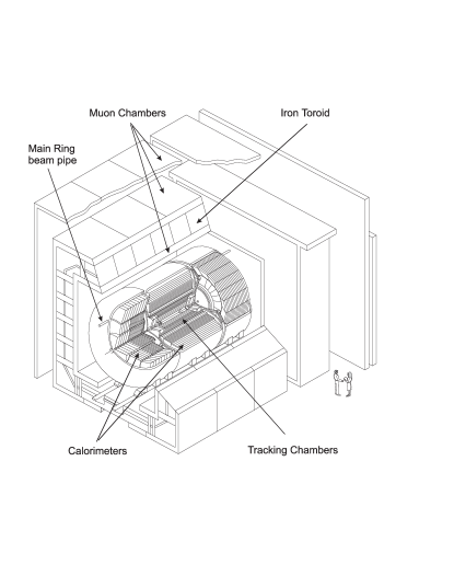
FIG. 1.: Isometric view of the DØ detector.

A Tracking system

The tracking system consists of a vertex drift chamber, a transition radiation detector, a central drift chamber, and two forward drift chambers. The system provides charged-particle tracking over the pseudorapidity region $|\eta|<$ 3.2, where $\eta$ = $-\ln({\tan{(\theta/2)}})$; $\theta$ and $\phi$ are, respectively, the polar and azimuthal angles relative to the proton beam axis. The resolution for charged particles is 2.5 mrad in $\phi$ and 28 mrad in $\theta$. The position of the interaction vertex along the beam direction ($z$) is determined typically to an accuracy of 8 mm.

B Calorimeter

The liquid-argon calorimeter, using uranium and stainless steel/copper absorber, is divided into three parts: a central calorimeter and two end calorimeters. Each part consists of an inner electromagnetic section, a fine hadronic section, and a coarse hadronic section, housed in a stainless steel cryostat. The intercryostat detector consists of scintillator tiles inserted in the space between the central and end calorimeter cryostats. In addition, “massless gaps”, installed inside both central and end calorimeters, are active readout cells, without absorber material, located inside the cryostat adjacent to the cryostat walls. The intercryostat detector and massless gaps improve the energy resolution for jets that straddle two cryostats. The calorimeter covers the pseudorapidity range $|\eta|<$ 4.2, and has a typical segmentation of 0.1 $\times$ 0.1 in $\Delta\eta$ $\times$ $\Delta\phi$. The energy resolution is $\delta(E)/E$ = 15%/$\sqrt{E{\rm(GeV)}}$ $\oplus$ 0.4% for electrons. For charged pions, the resolution is approximately 50%/$\sqrt{E{\rm(GeV)}}$, and for jets approximately 80%/$\sqrt{E{\rm(GeV)}}$ [10, 11].

As can be seen in Fig. 1, the Main Ring beam pipe penetrates the outer hadronic section of the calorimeters and the muon spectrometer. The Main Ring carries protons with energies between 8-150 GeV, and is used in antiproton production during the Tevatron $p\bar{p}$ running. Because of this, any losses from the Main Ring can produce backgrounds in the detector that must be removed.

C Muon spectrometer

The DØ experiment detects muons using proportional drift tubes (PDT) and an iron toroid. Because muons from top quark decays populate predominantly the central region, this analysis uses muon detection systems in the region $|\eta|<$ 1.

The combined material in the calorimeter and iron toroid has between 13 and 19 interaction lengths (the range-out energy for muons is approximately 3.5 GeV), making background from hadronic punchthrough negligible. Also, the small central tracking volume minimizes background from in-flight decays of pions and kaons.

A typical muon track is measured in four layers of PDTs before, and six layers after, the iron toroid. The six layers are constructed in two super-layers that are separated by about one meter to provide a good lever arm for measuring the muon momentum, $p$. The muon momentum is determined from its deflection angle in the magnetic field of the toroid. The momentum resolution is limited by multiple scattering in the traversed material, knowledge of the integrated magnetic field, and resolution on the measurement of the deflection angle. The resolution is roughly Gaussian in 1/$p$, and is approximately $\delta(1/p)$ = 0.18($p$-2)/$p^{2}\oplus$0.003 (with $p$ in GeV/$c$) for the algorithms that were used in this analysis.

IV Data Sample

This section describes the data sample and the simulated events for the $t\bar{t}$ signal used in our analysis.

A Initial selection criteria

The data sample was selected by imposing both hardware (Level 1) and software (Level 2) trigger requirements. These requirements were modified slightly over the course of the 1992–1996 run in order to accommodate the higher instantaneous luminosities later in the run. Table I indicates the three main running periods, the run numbers associated with these periods, and the integrated luminosity collected.

TABLE I.: Main running periods of the 1992–1996 run.

Run		Run	Integrated
Period	Dates	Numbers	Luminosity
Ia	1992–1993	50000–70000	13.0 pb-1
Ib	1993–1995	70000–94000	86.4 pb-1
Ic	1995–1996	94000–96000	10.8 pb-1

The hardware trigger required the presence of at least four calorimeter trigger towers (0.2 $\times$ 0.2 in $\Delta\eta$ $\times$ $\Delta\phi$), each with transverse energy $E_{T}>$ 5 GeV, for the Ia period. In the Ib and Ic periods, the $E_{T}$ requirement was raised to 7 GeV, and an additional requirement for at least three large tiles (0.8 $\times$ 1.6 in $\Delta\eta$ $\times$ $\Delta\phi$) with $E_{T}>$ 15 GeV was imposed. These were imposed to reduce the trigger rate and avoid saturating the bandwidth of the trigger system at high instantaneous luminosities ($\geq$ 10³¹ cm^-2 s^-1).

The software filter required five jets, defined by $\cal{R}$=$\sqrt{(\Delta\eta)^{2}+(\Delta\phi)^{2}}$=0.3 cones, with $|\eta|<$ 2.5 and $E_{T}>$ 10 GeV. Again, in order to reduce the data rate at high luminosities during the Ib period, a further condition was added requiring the scalar sum of the $E_{T}$ of all jets (defined as $H_{T}$) to be greater than 110 or 115 GeV, depending upon run number. This $H_{T}$ requirement was raised to 120 GeV during the Ic period. The effects of these changes on the acceptance for $t\bar{t}$ events were studied using Monte Carlo simulations, and were found to be negligible.

In addition to imposing trigger and filter requirements, a set of offline selection criteria was used to reduce the data sample to a manageable size without greatly affecting the acceptance for the $t\bar{t}$ signal. First, $H_{T}$ was required to be greater than 115 GeV, where the sum used ${\cal{R}}$=0.5 jets with $|\eta|<$ 2.5 and $E_{T}>$ 8 GeV. Also, requirements were imposed in order to eliminate events with spurious jets due to spray from the Main Ring or effects from noisy cells in the calorimeter [12, 13]. For example, Fig. 2 shows the imbalance in transverse energy, or missing $E_{T}$ (${\hbox{$E$\kern-6.00006pt\lower-0.43057pt\hbox{/}}}_{T}$), in the event versus the azimuthal angle ($\phi$) of the jet, before and after the rejection of Main Ring events. We see that our requirements have removed the spurious cluster of jets in the region where the Main Ring pierces the DØ detector (1.6 $<\phi<$ 1.8). Table II summarizes the impact of the trigger and initial reconstruction criteria on the $t\bar{t}$ signal for a top quark mass of 180 GeV/$c^{2}$.

TABLE II.: Initial criteria used for data selection.

			Cumulative
		Effective	Efficiency
General	Sequential	cross	($m_{t}$=180
Conditions	Requirements	section	GeV/$c^{2}$)
Level 1	Four trigger towers
trigger	$E_{T}>5,7$ GeV (Ia, Ib-c)	0.4 $\pm$ 0.1 $\mu$b	0.98
	Three large tiles
	$E_{T}>15$ GeV (Ib-c)
Level 2	Five ${\cal{R}}$=0.3 jets
filter	$|\eta|<$2.5, $E_{T}>10$ GeV	20 $\pm$ 5 nb	0.92
	$H_{T}>110,115$ GeV (Ib)
	$H_{T}>120$ GeV (Ic)
	$H_{T}>115$ GeV from
Offline	${\cal{R}}$=0.5 jet cones
	$|\eta|<$2.5, $E_{T}>8$ GeV	5.4 $\pm$ 1.3 nb	0.87
	Cuts for spurious jets

FIG. 2.: The effect of imposing requirements to reject Main Ring events. A scatter plot of missing $E_{T}$ versus $\phi$ for jets before (a), and after (b), imposing our Main Ring requirements.

B Jet algorithms

The jet algorithm is the fundamental analysis tool in the search for $t\bar{t}$ events in the all-jets mode. One of the most important considerations in choosing a jet algorithm is the efficiency for reconstructing the six primary $t\bar{t}$ decay products. The $\eta$ distribution of the jets from $t\bar{t}$ decays tends to be quite narrow, and therefore the $\cal{R}$ separation between adjacent jets is frequently small. When two jets are too close together, they may not be resolved, leading to reconstruction inefficiency.

Figure 3 shows the reconstruction efficiency for the cone jet algorithm [14] with various cone sizes for simulated $t\bar{t}$ events in the all-jets channel, as generated with the herwig Monte Carlo program[15]. Here, the definition of a quark includes any final state gluon radiation added back to the quark momentum. The matching of reconstructed jets to quarks relies on using combinations of the two that minimize the distance in $\cal{R}$ between them. A jet is considered to be matched only if that distance is less than $\Delta\cal{R}$=0.5, the energy of the jet is within a factor of two of the quark energy, and the reconstructed jet $E_{T}$ is greater than 10 GeV.

Figures 3(a) and 3(b) show how the reconstruction efficiency depends on quark $E_{T}$ and $\eta$ for the cone algorithm with different cone sizes. The $\cal{R}$=0.3 cone algorithm shows a higher jet reconstruction efficiency than the larger cone algorithms. In the central region, the $\cal{R}$=0.3 cone algorithm has an efficiency of 94%, while the $\cal{R}$=0.5 and $\cal{R}$=0.7 cone algorithms are 90% and 81% efficient, respectively. Given an average efficiency $\epsilon$ for reconstructing a single jet, the reconstruction efficiency for finding $t\bar{t}$ events (with six or more jets) will be of the order of $\epsilon^{6}$. Therefore, larger cone sizes are less efficient in the multijet environment.

FIG. 3.: Jet reconstruction for $t\bar{t}$ Monte Carlo events (herwig, $m_{t}$ = 175 GeV/$c^{2}$) for various cone sizes: ${\cal{R}}$=0.3 (open squares), ${\cal{R}}$=0.5 (full circles), and ${\cal{R}}$=0.7 (open circles). (a) Jet finding efficiency versus quark $E_{T}$. (b) Jet finding efficiency versus quark $\eta$. (c) Reconstructed jet energy versus that of the input quark. (d) Reconstructed mass of the top quark from correct jet combinations, where the areas reflect the relative efficiencies.

Figure 3(c) shows the correspondence between parton and jet energies found for various cone algorithms, after DØ jet energy corrections are applied (see next section). Linear fits to the quark-jet correlation in energy are shown in Fig. 3(c) for the three cone algorithms. Figure 3(d) shows the three-jet invariant mass for the correct combinations of jets matching top and antitop quarks. The areas of the mass distributions reflect the event reconstruction efficiencies for different algorithms.

The shift in the reconstructed mass from the input mass of the top quark (175 GeV/$c^{2}$) shows that the jet algorithms are not equivalent. The shift in three-jet mass from the nominal input top quark mass increases as the cone radius is decreased. The widths of the mass distributions are not very sensitive to the choice of cone size. The overall root-mean-square, rms, spread in reconstructed mass for correct combinations of jets is approximately 10% of the mass.

In summary, there are two competing effects when choosing the optimal jet cone size. Smaller cone sizes are better able to resolve separate jets, but do not do as well at reconstructing jet energy. However, the ability to resolve individual jets was deemed of higher importance in the search for a signal. Hence the $\cal{R}$=0.3 cone algorithm is preferred for analyzing multijet events. But, due to the relatively large shift in the jet energy for the $\cal{R}$=0.3 cone algorithm, we chose to use the $\cal{R}$=0.5 cone algorithm for calculating some quantities that emphasize energy response at the expense of jet efficiency. Jets with $E_{T}~{}<$ 8 GeV, before application of energy corrections (see Sec. IV.C), were discarded.

C Jet energy correction

DØ has developed a correction procedure [16] to calibrate jet energies, which is applied to both data and Monte Carlo. The underlying assumption is that the true jet energy, $E_{\rm ptcl}$, is the sum of the energies of all final state particles entering the cone algorithm applied at the calorimeter level. $E_{\rm ptcl}$ is obtained from the energy measured in the calorimeter, $E_{\rm meas}$, as follows:

$$E_{\rm ptcl}=\frac{E_{\rm meas}-E_{\rm O}({\cal R},\eta,{\cal L})}{R(\eta,E,{\sc rms})S({\cal R},\eta,E)}\,,$$ (1)

where:

• $E_{\rm O}({\cal R},\eta,{\cal L})$ is an offset, which includes the physics of the underlying event, noise from the radioactive decay of the uranium absorber, the effect of previous crossings (pile-up), and the contribution of additional contemporaneous $p\bar{p}$ interactions. The physics of the underlying event is defined as the energy contributed by spectators to the hard parton interaction which resulted in the high-$p_{T}$ event. This offset increases as a function of the cone size ${\cal R}$. It also depends on $\eta$ and on the instantaneous luminosity, ${\cal L}$, which is related to the contribution from the additional $p\bar{p}$ interactions.

• $R(\eta,E,{\sc rms})$ is the energy response of the calorimeter. It is nearly independent of the jet cone size, ${\cal R}$, but does depend on the rms width of the jet. The width dependence accounts for differences in the calorimeter response to narrow jets, which fragmented into fewer particles (of, on average, higher energy) than broader jets, with larger particle multiplicities. Because the various detector components are not identical, $R$ also depends on detector $\eta$. $R$ is typically less than one, due to energy loss in the uninstrumented regions between modules, differences between the electromagnetic ($e$) and hadronic response ($h$) of the detector ($e/h>1$), and module-to-module inhomogeneities.

• $S({\cal R},\eta,E)$ is the fraction of the jet energy that is deposited inside the algorithm cone. Since the jet energy is corrected back to the particle level, the effects of calorimeter showering must be removed. $S$ is less than one, meaning that the effect of showering is a net flux of energy from inside to outside the cone. $S$ depends strongly on the cone size ${\cal R}$, energy, and $\eta$.

D Characteristics of jets

Comparisons of jet properties (jet multiplicity, inclusive jet $E_{T}$, $\eta$, and $\phi$, for $\cal{R}$=0.3 cones) are shown in Fig. 4 for data from the Ia and Ib periods (see Table I) and for $t\bar{t}$ Monte Carlo. Only jets with $E_{T}>$ 10 GeV and $|\eta|<2$ are included in the comparison. The results from Ia and Ib are in good agreement, although Ib typically had higher instantaneous luminosity.

Figure 4(a) shows that for events with six jets, the background (i.e., data) is at least three orders of magnitude larger than the expected $t\bar{t}$ signal. The peak at five jets is the result of the initial event selection (see Table II). The inclusive jet $E_{T}$ spectrum in Fig. 4(b) falls exponentially at about the same rate for signal as for data, and the signal is consistently three orders of magnitude below the data. In Fig. 4(c), the distributions of jet $\eta$ are normalized to the same area for signal and data. The signal is concentrated in the central region, while the data extend to higher $\eta$. There is a difference of the order of 10% between Ia and Ib in the intercryostat region ($|\eta|\approx$ 1.2) due to improvements in the Ib period. Figure 4(d) shows that the $\phi$ distribution of jets is isotropic, except for a 5% suppression in the region of the Main Ring. The Monte Carlo does not simulate the effects of the Main Ring, and consequently has no apparent structure in $\phi$.

FIG. 4.: Properties of jets with $\cal{R}$=0.3 cones. Data from the Ia (histograms) and Ib (circles) periods, and $t\bar{t}$ herwig for $m_{t}$=175 GeV/$c^{2}$ (shaded histograms). Only jets with $E_{T}$ $>$ 10 GeV and $|\eta|<2$ are included. Distributions in (a) jet multiplicity and (b) jet $E_{T}$ are each normalized to the expected number of events in 110.3 pb^-1 of data, while distributions in (c) jet $|\eta|$ and (d) jet $\phi$ are normalized to the same area.

E Simulation of $t\bar{t}$ events

The simulation of $t\bar{t}$ events plays an important role in extracting a signal in the presence of significant background. It is necessary, therefore, to have a good description of the production and decay of $t\bar{t}$ events in order to calculate detector acceptances accurately and to develop methods to identify $t\bar{t}$ events in the data.

The $t\bar{t}$ events were generated for top quark masses between 120 and 220 GeV/$c^{2}$ for the reaction $p\bar{p}\rightarrow t\bar{t}+X$ using herwig as a primary model and isajet [18] as a check. The underlying assumptions in the fragmentation of partons are different in the two programs. The generated events were put through the DØ shower library [19], a fast detector simulation package based on geant [20], which contains the effects of cracks and other dead material in the DØ calorimeter, and provides accurate shower simulation. The geant simulation has been tuned to achieve a good match between generated single-particle characteristics and observed data [21]. Events were subsequently digitized, passed through the DØ reconstruction program [10], and subjected to the same selection criteria as the data (see Table II). Events passing these criteria served as the model for our studies of $t\bar{t}$ properties.

Generally, acceptances for $t\bar{t}$ production as calculated with herwig or isajet agree to within 10%, and any differences between the two are incorporated in the final systematic uncertainties. As an illustration of the discrepancies, we show in Fig. 5 distributions of jet multiplicity, jet $\eta$, the $E_{T}$ of the leading jet, and the fifth highest jet $E_{T}$ for herwig and isajet. Except for jet multiplicity, these distributions are in good agreement. It has been shown [11] that isajet produces more gluon radiation than herwig, in accord with our results in Fig. 5(a).

FIG. 5.: Comparisons of isajet (circles) and herwig (histograms) for an input top quark mass of 175 GeV/$c^{2}$, and jets with $\cal{R}$=0.3 cones, for (a) jet multiplicity, (b) jet $\eta$, (c) $E_{T}$ of leading jet, and (d) fifth highest jet $E_{T}$. Bars on the points indicate statistical uncertainties (similar uncertainties, although not shown, apply for the histograms). The results from isajet and herwig in (a)–(d) are normalized to the same area.

V Kinematic Parameters

The principal background to the $t\bar{t}$ signal is QCD multijet production, which is dominated by a $2\rightarrow 2$ parton process with additional jets produced through gluon radiation. Therefore, the background tends to have jets that are more forward-backward in rapidity. The additional jets are generally lower in $E_{T}$ (i.e., softer) than the initial outgoing parent partons. Furthermore, this extra radiation tends to lie in a plane formed by the incoming beam and the two leading jets.

Because the mass of the top quark is large, the characteristic energy scale (commonly called $Q^{2}$) of the $t\bar{t}$ event is significantly larger than that of the average QCD background event. This means that $t\bar{t}$ events generally have jets with higher $E_{T}$, and have larger multijet invariant masses.

Extracting a signal from data dominated by background requires the use of global kinematic parameters based on these differences. Employing such parameters helps to differentiate between the $t\bar{t}$ signal and background. We can summarize the salient features of the background, relative to the $t\bar{t}$ signal, as follows:

• The overall energy scale is lower; leading jets have lower $E_{T}$; multijet invariant masses are smaller.

• The additional radiated jets are softer (have lower $E_{T}$).

• The event shape is more planar (less spherical).

• The jets are more forward-backward in rapidity (less central).

We defined two or more kinematic parameters that quantified aspects of each property. Only the most effective of these were used and these are discussed below. We found that, in general, better discrimination was achieved using $\cal{R}$=0.3 cone jets (with $|\eta|<2.0$ and $E_{T}>15$ GeV) than $\cal{R}$=0.5 cone jets. However, in some instances, $\cal{R}$=0.5 cone jets were used, and this is noted where it occurs.

Although correlations exist between many of the kinematic parameters, each includes useful information not fully contained in any of the others. These correlations are presented in Sec. VI.D.

A Parameters sensitive to energy scale

Any parameter that depends on the energy scale of the jets is also sensitive to the mass of the top quark. These “mass sensitive” parameters usually provide better discrimination against QCD background than other parameters that provide only a measure of some topological feature. Three mass sensitive parameters are:

1. $H_{T}$
   The sum of the transverse energies of jets in a given event characterizes the transverse energy flow, and is defined as:

   $$H_{T}=\sum_{j=1}^{N_{\rm jets}}E_{T_{j}}$$ (2)

   where $E_{T_{j}}$ is the transverse energy of the $j$th jet, as ordered in decreasing jet $E_{T}$ rank, and $N_{\rm jets}$ is the number of jets in the event.

2. $\sqrt{\hat{s}}$
   This parameter is the invariant mass of the $N_{\rm jets}$ system.

3. $E_{T_{1}}$/$H_{T}$
   $E_{T_{1}}$ is the transverse energy of the $\cal{R}$=0.5 cone jet with highest $E_{T}$. This parameter characterizes the $E_{T}$ fraction carried by the leading jet, and tends to be high for QCD background. The $t\bar{t}$ events are likely to have transverse energy roughly equipartitioned among all six jets, and hence the leading $E_{T}$ jet is, on average, fractionally softer.

Figure 6 shows the distributions of $H_{T}$, $\sqrt{\hat{s}}$, and $E_{T_{1}}$/$H_{T}$, each of which reveals significant discrimination between signal and background. This and subsequent figures for the parameters are shown both normalized to cross section, and normalized to unity.

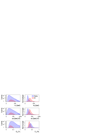
FIG. 6.: The $H_{T}$, $\sqrt{\hat{s}}$, and $E_{T_{1}}$/$H_{T}$ distributions for data (predominantly background) and for herwig $t\bar{t}$ generated at a top quark mass of 175 GeV/$c^{2}$. Each plot on the left is normalized according to the expected number of events. On the right the plots are normalized to unity and reveal significant discrimination between signal and background.

B Parameters sensitive to additional radiation

As previously noted, the QCD background is primarily a $2\rightarrow 2$ parton process that contains additional radiated gluons. These gluons tend to be much softer than the leading partons, and therefore the jets associated with this radiation tend to have smaller $E_{T}$. Three parameters that measure the hardness of this radiation are:

1. $H_{T}^{3j}$
   This variable is defined as[12, 13]:

   $$H_{T}^{3j}=H_{T}-E_{T_{1}}-E_{T_{2}}$$ (3)

   where $E_{T_{1}}$ and $E_{T_{2}}$ are the transverse energies of the two leading (highest $E_{T}$) jets. By subtracting the $E_{T}$ of the two leading jets, what remains is a better measure of any additional gluon radiation in QCD events, enhancing the discrimination between $t\bar{t}$ signal and QCD background.

2. $N_{\rm jets}^{A}$
   An average jet count parameter, $N_{\rm jets}^{A}$, provides a way to parameterize the number of jets in an event, while taking account of the hardness of these jets. We define:

   $$N_{\rm jets}^{A}={{\displaystyle\int^{55}_{15}}E_{T}^{\rm thr}N(E_{T}^{\rm thr})\,dE_{T}^{\rm thr}\over{\displaystyle\int^{55}_{15}}E_{T}^{\rm thr}\,dE_{T}^{\rm thr}}$$ (4)

   where $N(E_{T}^{\rm thr})$ is the number of jets in a given event with $|\eta|<2.0$ and $E_{T}$ greater than some threshold, $E_{T}^{\rm thr}$ in GeV. Therefore, this parameter corresponds to the number of jets, but is more sensitive to jets of higher $E_{T}$ than just a simple jet count above some given threshold.

3. $E_{T_{5,6}}$
   The transverse energies of the fifth jet, $E_{T_{5}}$, and sixth jet, $E_{T_{6}}$, are also useful in discriminating QCD background from $t\bar{t}$ events. Our final selection (see Sec. VII(a)) requires at least six jets. For background these usually correspond to soft radiation. The variable chosen is:

   $$E_{T_{5,6}}=\sqrt{E_{T_{5}}~{}E_{T_{6}}}.$$ (5)

Figure 7 shows distributions of $H_{T}^{3j}$, $N_{\rm jets}^{A}$ and $E_{T_{5,6}}$. Again, these variables are effective in differentiating between signal and background.

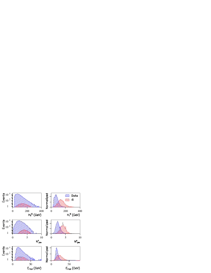
FIG. 7.: The $H_{T}^{3j}$, $N_{\rm jets}^{A}$, and $E_{T_{5,6}}$ distributions for data (predominantly background) and for herwig $t\bar{t}$ events. Each distribution is normalized to the expected number of events (left) and to unity (right).

C Aplanarity and sphericity

The direction and shape of the momentum flow of jets in $t\bar{t}$ production are different from those in QCD background. These differences can be quantified using event-shape parameters[22]. For each event, we define the normalized momentum tensor $M_{ab}$:

$$M_{ab}=\sum_{j}^{N_{\rm jets}}p_{ja}p_{jb}/\sum_{j}^{N_{\rm jets}}p_{j}^{2}$$ (6)

where $a$ and $b$ run over the $x,y,z$ components (indices of the tensor), and $j$ runs over the number of jets in an event. As is clear from its definition, $M_{ab}$ is a symmetric matrix that is always diagonalizable, and has positive-definite eigenvalues ($Q_{1},Q_{2},Q_{3}$) satisfying the conditions:

$$Q_{1}+Q_{2}+Q_{3}=1~{}~{}~{}{\rm and}~{}~{}~{}0\leq Q_{1}\leq Q_{2}\leq Q_{3}.$$ (7)

The equation $Q_{1}+Q_{2}+Q_{3}=1$ represents a plane in a space spanned by $Q_{1},Q_{2}$, and $Q_{3}$, and the inequality restricts the range of each eigenvalue, as shown in Fig. 8:

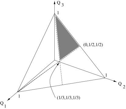
FIG. 8.: The allowed range of normalized momentum tensor eigenvalues in the space spanned by the $Q_{i}$.

$$0\leq Q_{1}\leq\frac{1}{3},$$ (8)

$$0\leq Q_{2}\leq\frac{1}{2},$$ (9)

$$\frac{1}{3}\leq Q_{3}\leq 1.$$ (10)

The magnitude of any $Q_{i}$ represents the portion of momentum flow in the direction of the $i^{th}$ eigenvector. Limiting event shapes can therefore be characterized as follows:

• Linear : $Q_{1}=Q_{2}=0$ and $Q_{3}$ = 1.

• Planar : $Q_{1}=0$ and $Q_{2}=Q_{3}$ = $\frac{1}{2}$.

• Spherical : $Q_{1}=Q_{2}=Q_{3}$ = $\frac{1}{3}$.

The aplanarity ($\cal{A}$) and sphericity ($\cal{S}$) parameters that we use are defined as follows:

1. ${\cal{A}}=\frac{3}{2}Q_{1}$,

2. ${\cal{S}}=\frac{3}{2}\left(Q_{1}+Q_{2}\right)$,

with $0\leq{\cal{A}}\leq 0.5$ and $0\leq{\cal{S}}\leq 1$.

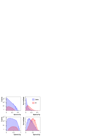
FIG. 9.: The aplanarity and sphericity distributions for data (predominantly background), and for herwig $t\bar{t}$ events. Each distribution is normalized to the expected number of events (left) and to unity (right).

Top quark ($t\bar{t}$) events tend to have higher aplanarity and sphericity than background events. We calculate $\cal{A}$ and $\cal{S}$ in the $p\bar{p}$ collision frame; little difference is found using the parton center of mass frame. Distributions of $\cal{A}$ and $\cal{S}$ for herwig $t\bar{t}$ events for $m_{t}$=175 GeV/$c^{2}$ and for data are shown in Fig. 9.

D Parameters sensitive to rapidity distributions

1. ${\cal{C}}$
   The centrality (${\cal{C}}$) parameter is defined as:

   $${\cal{C}}=\frac{H_{T}}{H_{E}},$$ (12)

   where

   $$H_{E}=\sum_{j=1}^{N_{\rm jets}}E_{j}.$$ (13)

   Centrality is similar to $H_{T}$, characterizing the transverse energy in events, but is normalized in such a way that it depends only weakly on the mass of the top quark.

2. $\left<\eta^{2}\right>$
   To good approximation, the $\eta$ distribution for jets in $t\bar{t}$ events is normally distributed about zero with an rms, $\sigma_{\eta}$, close to unity. With typically six or more jets in an event, the rms of the jet $\eta$ distribution can be a useful discriminator. The $\left<\eta^{2}\right>$ variable is defined using only the leading six jets. We use $\cal{R}$=0.5 cone jets for this variable.

   We calculate $\left<\eta^{2}\right>$ by taking the square of the difference between each jet $\eta$ and the $E_{T}$-weighted mean, $\bar{\eta}$, weighted by a factor ${\cal W}(E_{T})$. ${\cal W}(E_{T})$ depends upon the difference in rms between $t\bar{t}$ signal ($\sigma_{\eta}^{t\bar{t}}$) and background ($\sigma_{\eta}^{\rm bkg}$), and is larger at those $E_{T}$ values where signal and background are expected to differ. The $\left<\eta^{2}\right>$ parameter is given by:

   $${\rm\left<\eta^{2}\right>}=\frac{\sum_{j=1}^{6}{\cal{W}}(E_{T_{j}})\left(\eta_{j}-\bar{\eta}\right)^{2}}{\sum_{j=1}^{6}{\cal{W}}(E_{T_{j}})},$$ (14)

   where

   $${\cal{W}}(E_{T})=\frac{\sigma_{\eta}^{t\bar{t}}(E_{T})-\sigma_{\eta}^{\rm bkg}(E_{T})}{\sigma_{\eta}^{t\bar{t}}(E_{T})}\quad{\rm and}$$ (15)

   $$\bar{\eta}=\frac{1}{H_{T}}\sum_{j=1}^{N_{\rm jets}}E_{T_{j}}~{}\eta_{j}.$$ (16)

   Note that both $\sigma_{\eta}^{t\bar{t}}(E_{T})$ and $\sigma_{\eta}^{\rm bkg}(E_{T})$ depend on the $E_{T}$ of the jets in the $\eta$ distribution. Jets with lower $E_{T}$ tend to be at larger values of $|\eta|$, and consequently $\sigma_{\eta}$ decreases with increasing $E_{T}$. The QCD multijet background has a broader distribution in the $\left<\eta^{2}\right>$ variable than the $t\bar{t}$ signal.

The ${\cal C}$ and $\left<\eta^{2}\right>$ distributions are shown in Fig. 10, for $m_{t}$ = 175 GeV/$c^{2}$.

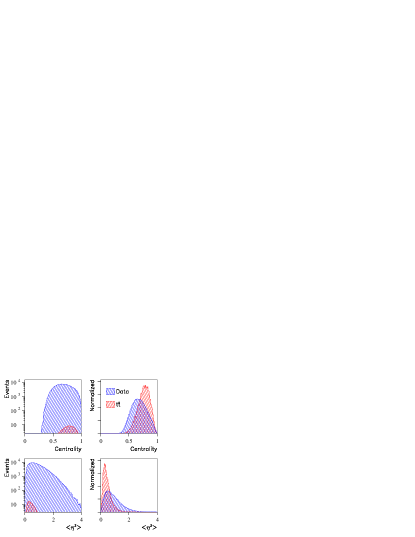
FIG. 10.: The centrality and $\left<\eta^{2}\right>$ distributions for data (predominantly background) and for herwig $t\bar{t}$ events. Each distribution is normalized to the expected number of events (left) and to unity (right).

The above ten kinematic variables are employed as inputs to the first neural network. The output of this network is an input to the second (and final) neural network, whose three other inputs are described in the following section.

VI Event Structure Variables

In addition to the kinematic and topological characteristics examined in Sec. V, there are other differences between the $t\bar{t}$ signal and the QCD multijet background that we will exploit in extracting the $t\bar{t}$ signal.

A $p_{T}$ of tagging muon

The $p_{T}$ of the tagging muon gives further discrimination between $t\bar{t}$ signal and QCD background. Not only does the fragmentation of $b$ quarks produce higher $p_{T}$ objects, but the $b$ quark is also more energetic in $t\bar{t}$ events than in background. Thus, the mean muon $p_{T}$, $p_{T}^{\mu}$, is significantly larger in $t\bar{t}$ events. Figure 11 shows the muon $p_{T}$ spectra. Figure 11(a) compares the muon $p_{T}$ in herwig and isajet $t\bar{t}$ events, which shows that the muon $p_{T}$ spectrum is modeled consistently by Monte Carlo. Figure 11(b) compares herwig $t\bar{t}$ events and data (predominantly background). These results show that the $p_{T}$ of the muon can serve as a useful tool in differentiating between signal and background.

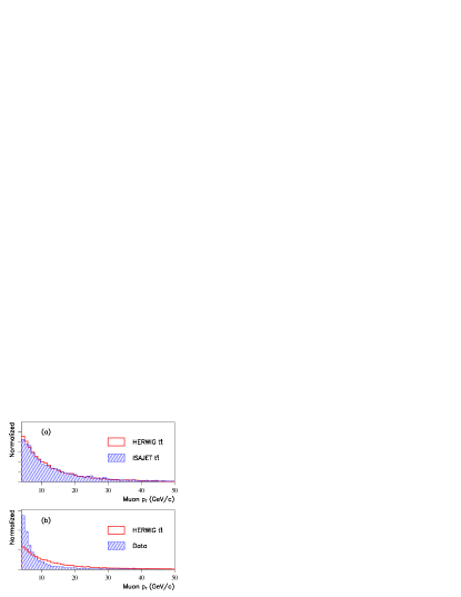
FIG. 11.: Comparison of muon $p_{T}$ spectra for (a) herwig and isajet $t\bar{t}$ events, and (b) herwig $t\bar{t}$ events and data. These distributions have been normalized to unity.

B Widths of jets

At the simplest level, each $t(\bar{t})$ quark decays into a $b(\bar{b})$ quark and a $W^{+}(W^{-})$ boson, with each $W$ boson decaying into light quarks. Barring extra gluon bremsstrahlung, this represents six quark-jets in the final state. The average jet multiplicity for herwig $t\bar{t}$ events ($m_{t}$=175 GeV/$c^{2}$) using our selection criteria is 6.9, implying that the contribution from gluons is relatively small. Conversely, jets in the QCD multijet background originate predominantly from gluon radiation. Although gluon splitting can take place, producing both quark and gluon jets, it is expected that gluons dominate QCD multijet production.

QCD predicts substantial differences between quark jets and gluon jets and, in fact, observed differences in quark and gluon jet widths have been reported by experiments at the KEK $e^{+}e^{-}$ collider (TRISTAN)[23] and the CERN $e^{+}e^{-}$ collider (LEP)[24]. Parton shower Monte Carlos such as herwig have been shown to reproduce the widths observed in data [24], although herwig has been found to slightly underestimate jet widths at the Fermilab Tevatron [25]. We found that by applying a correction of 3% to the widths, herwig QCD Monte Carlo reproduces the observed distributions in the width of the jets. Further studies have shown that the kinematic distributions of the multijet background are also well modeled using herwig. We have therefore chosen herwig as the generator for studying jet widths, with a 3% correction applied to the widths of each jet.

Figure 12(a) shows the mean width of 0.5 cone jets versus jet $E_{T}$ for multijet data and herwig QCD and Fig. 12(b) compares the data to herwig $t\bar{t}$. Here, the jet width is:

$$\sigma_{\rm jet}=\sqrt{\sigma_{\eta}^{2}+\sigma_{\phi}^{2}},$$ (17)

where $\sigma_{\eta}$ and $\sigma_{\phi}$ are the transverse energy weighted rms widths in $\eta$ and $\phi$, respectively, and are calculated using the ($\eta$,$\phi$) positions of each calorimeter bin (0.1 $\times$ 0.1 in $\Delta\eta$ $\times$ $\Delta\phi$) weighted by the transverse energy in that bin. In order to account for the broadening of jets from additional minimum bias interactions which could overlap an event, corrections were applied to the widths of each jet in the event. These corrections were typically a few percent, and depended, among other factors, upon the instantaneous luminosity during that event. These corrections were determined by assuming that the energy coming from minimum bias interactions was uniformly distributed in $\Delta\eta$ and $\Delta\phi$, and therefore the measured rms of a jet was the sum in quadrature of its true rms and the rms of a uniform distribution.

It is clear from Fig. 12(a) that herwig QCD describes the widths observed in the data, and the herwig $t\bar{t}$ has significantly narrower jets. This suggests that the difference may be due to the different mix of gluons and quarks in the two processes.

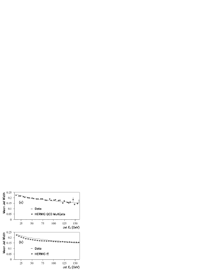
FIG. 12.: The mean width of 0.5 cone jets versus their $E_{T}$ for (a) data (bars) and herwig QCD (stars), and (b) data (bars) and herwig $t\bar{t}$ (stars).

For Monte Carlo it is possible to match initial state quarks to final state reconstructed jets because the herwig $t\bar{t}$ events are relatively simple. The mapping between quarks and jets requires a tight match in $\Delta\cal{R}$ between the initial quark and the jet, as well as a reasonable match in energy. The following criteria were employed to define Monte Carlo “quark-like jets”:

• Good quality 0.5 cone jet, reconstructed without merging (not formed from two or more adjacent jets) and with $|\eta|~{}\leq$ 2.5,

• Distance between initial quark and its reconstructed jet to be $\Delta\cal{R}$ $\leq$ 0.05,

• The difference in energy between the quark and the jet $\Delta E$ $\leq$ $\sqrt{E_{\rm quark}}$ ($E$ in GeV).

Monte Carlo “gluon-like jets” were defined to be good quality jets, without merging, but where the separation distance to the nearest quark was $\Delta\cal{R}$ $\geq$ 1. Imposing these criteria, the distributions in the jet rms widths are shown in Fig. 13. To guide the eye, Gaussian fits have been superimposed on the distributions. With these definitions, it appears that gluon-like jets are 20-30% wider than quark-like jets.

FIG. 13.: Distributions in jet rms width, $\sigma_{\rm jet}$, for herwig quark-like jets (solid) and the gluon-like jets (dashed) for (a) $5<E_{T}<25$ GeV, (b) $20<E_{T}<40$ GeV, (c) $35<E_{T}<55$ GeV, (d) $50<E_{T}<70$ GeV, (e) $65<E_{T}<85$ GeV, and (f) $80<E_{T}<100$ GeV. These distributions were normalized to have equal numbers (1000) of events.

Figure 13 suggests that the jet rms distributions for these definitions of quark/gluon jets can be approximated by Gaussians. A Fisher discriminant can be used to differentiate statistically between any two such distributions. We defined a Fisher discriminant, ${\cal F}_{\rm jet}$, in terms of the individual jet width $\sigma_{\rm jet}$ and the width expected for gluon-like ($\sigma_{\rm gluon}$) and quark-like ($\sigma_{\rm quark}$) jets, as follows:

$${\cal F}_{\rm jet}=\frac{(\sigma_{\rm jet}-\sigma_{\rm quark}(E_{T}))^{2}}{\sigma^{2}_{\rm quark}(E_{T})}-\frac{(\sigma_{\rm jet}-\sigma_{\rm gluon}(E_{T}))^{2}}{\sigma^{2}_{\rm gluon}(E_{T})}$$ (18)

We used this single parameter to characterize the quark-like or gluon-like essence of a jet. This discriminant is summed over the four unmerged jets with the smallest values of ${\cal F}_{\rm jet}$ in an event to form a variable ${\cal F}$ which reflects whether the event is more $t\bar{t}$-like (signal) or more QCD-like (background). Summing only over the four smallest values of ${\cal F}_{\rm jet}$ (most quark-like jets), according to Monte Carlo, optimizes the discrimination. This summed discriminant, ${\cal F}$, will be used in our search for $t\bar{t}$ signal in the all-jets channel. The distributions of ${\cal F}$ are shown in Fig. 14. It is known that jet widths are not as well modeled in isajet [26], and we have, therefore, based this discriminant only on the herwig generator. Figure 14(a) shows ${\cal F}$ for data and herwig QCD, and Fig. 14(b) shows ${\cal F}$ for data and herwig $t\bar{t}\rightarrow$ all-jets. Comparison shows that the jets in data are significantly wider, and are more consistent with herwig QCD than with herwig $t\bar{t}$.

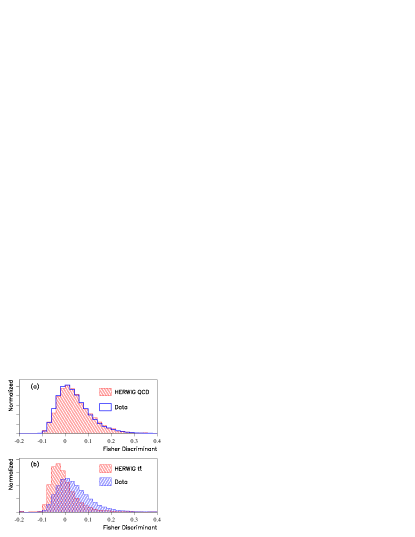
FIG. 14.: Distributions of ${\cal F}$ for, (a) data (predominantly background) and herwig QCD, and (b) data and herwig $t\bar{t}$ events.

C Mass likelihood parameter

A mass likelihood variable, ${\cal M}$, defined below, provides good discrimination between signal and background by requiring two jet pairs that are consistent with the $W$ boson mass, and two $W$ + jet pairs that are consistent with a single top quark mass of any value. Since there are no high-$p_{T}$ leptons in the all-jets channel, and hence no high-$p_{T}$ neutrinos, the event is in principle fully reconstructible. The presence of two $W$ bosons in $t\bar{t}$ events provides significant rejection against QCD background. A further requirement that the two reconstructed top quarks have equal masses provides some additional discrimination. ${\cal M}$ is defined as a $\chi^{2}$-like object:

$${\cal M}=\frac{(M_{W_{1}}-M_{W})^{2}}{\sigma_{W}^{2}}+\frac{(M_{W_{2}}-M_{W})^{2}}{\sigma_{W}^{2}}+\frac{(m_{t_{1}}-m_{t_{2}})^{2}}{\sigma_{t}^{2}},$$ (19)

where $M_{W_{1}}$ ($M_{W_{2}}$) is the mass of the two ${\cal{R}}$=0.5 cone jets corresponding to the $W$ boson from the first (second) top quark, of mass $m_{t_{1}}$ ($m_{t_{2}}$). The parameters $M_{W}$, $\sigma_{W}$ and $\sigma_{t}$ were fixed at 80, 16 and 62 GeV/$c^{2}$, respectively. The last two values approximate the full widths of the two distributions, and taking them to be constant simplifies the calculation.

The ${\cal M}$ variable is calculated by looping over combinations of jets, and assigning all jets with $|\eta|~{}\leq$ 2.5 to one of the $W$ bosons or $b$ quarks from the two top quark decays. The smallest value of ${\cal M}$ is selected as the discriminator. To reduce the number of combinations, two jets are assigned to each $W$ boson, and one to the $b$ quark from one of the two top quarks. Jets from the $W$ boson are required to have $E_{T}>10$ GeV, while those from the $b$ quark must have $E_{T}>15$ GeV. All remaining jets are assigned to the $b$ quark from the second top quark. To keep $b$-tagged events on the same footing as untagged events, no a priori assignment is made between tagged jets and $b$ quarks. Since in the top quark rest frame the $W$ boson and the $b$ quark have equal momenta, the $E_{T}$ of $W$ bosons and $b$-jets are more similar than for QCD background. The following criterion helps further reduce combinatorics:

• $E_{T(W_{1})}~{}+~{}E_{T(W_{2})}~{}\leq~{}0.65~{}H_{T}$,

where $E_{T(W_{1})}$ ($E_{T(W_{2})}$) is the $E_{T}$ from the vector sum of two jet momenta assigned to the $W$ boson from the first (second) top quark. Although there are other possible algorithms for assigning jets to the two top quarks, the discrimination in the ${\cal M}$ variable is not very sensitive to the choice of reasonable algorithms.

The distributions in the ${\cal M}$ variable are shown in Fig. 15. Figure 15(a) compares the ${\cal M}$ variable in herwig and isajet $t\bar{t}$ events ($m_{t}$=175 GeV/$c^{2}$). Figure 15(b) compares herwig QCD and the data (predominantly background). Figure 15(c) compares herwig $t\bar{t}$ events and data. These plots show that this variable is modeled consistently by the two $t\bar{t}$ Monte Carlos, that herwig QCD models the background well, and that ${\cal M}$ is useful in discriminating between signal and background.

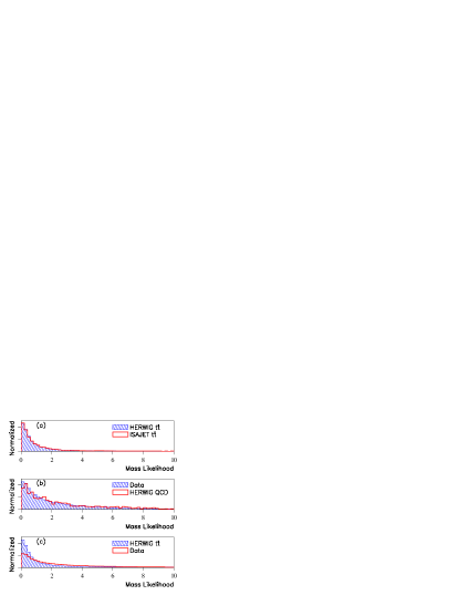
FIG. 15.: Distribution in mass likelihood parameter for (a) herwig and isajet $t\bar{t}$ events, (b) herwig QCD and data, and (c) herwig $t\bar{t}$ events and data. These distributions were normalized to unity.

D Correlations between parameters

A summary of the 13 parameters used in this analysis is given in Table III. The first ten parameters are simple kinematic variables, and are correlated. To quantify the degree of correlation between any two variables $x$ and $y$, we define a linear correlation coefficient, $r$ as[27]:

TABLE III.: The 13 variables used in the neural network analysis, the jet cone size employed and the $t\bar{t}$ event characteristic upon which it discriminates are given.

Variable	Description	Cone	Characteristic
$H_{T}$	Total transverse energy	0.3	Energy
$\sqrt{\hat{s}}$	Total $t\bar{t}$	0.3	Energy
	center-of-mass energy		Energy
$E_{T_{1}}$/$H_{T}$	Leading jet transverse	0.5/0.3	Energy
	energy fraction
$H_{T}^{3j}$	Transverse energy of	0.3	Radiation
	non-leading jets
$N_{\rm jets}^{A}$	Weighted number of jets	0.3	Radiation
$E_{T_{5,6}}$	$E_{T}$ of 5th and	0.3	Radiation
	6th jets
${\cal{A}}$	Aplanarity	0.3	Topology
${\cal{S}}$	Sphericity	0.3	Topology
${\cal{C}}$	Centrality	0.3	Topology
$\left<\eta^{2}\right>$	Rapidity distribution	0.5	Topology
$p_{T}^{\mu}$	$p_{T}$ of tagging muon	-	Event
			Structure
${\cal F}$	Fisher discriminant	0.5	Event
	based on jet widths		Structure
${\cal M}$	Mass likelihood	0.5	Event
			Structure

$$r={{\displaystyle N\sum}x_{i}y_{i}-\sum x_{i}\sum y_{i}\over\left[{\displaystyle N}\sum x_{i}^{2}-(\sum x_{i})^{2}\right]^{1/2}\left[N\sum y_{i}^{2}-(\sum y_{i})^{2}\right]^{1/2}}.$$ (20)

The value of $r$ ranges from 0, when there is no correlation, to $\pm$1, when there is complete correlation or anticorrelation. Table IV shows the average correlations among 13 parameters defined in Sec. V and Sec. VI for data. These are average correlation coefficients; local correlations can vary significantly, depending upon the region of multivariate space. Note that the parameters $p_{T}^{\mu}$, ${\cal F}$, and ${\cal M}$ have relatively small correlations with the other kinematic parameters.

TABLE IV.: Average correlations among the 13 parameters for data.

	$H_{T}$	$\sqrt{\hat{s}}$	$E_{T_{1}}/H_{T}$	$H_{T}^{3j}$	$N_{\rm jets}^{A}$	$E_{T_{5,6}}$	$\cal{A}$	$\cal{S}$	${\cal{C}}$	$\left<\eta^{2}\right>$	$p_{T}^{\mu}$	${\cal F}$	${\cal M}$
$H_{T}$	1	0.80	–0.14	0.71	0.76	0.39	0.01	0.	0.17	–0.31	0.04	–0.04	0.05
$\sqrt{\hat{s}}$		1	–0.20	0.64	0.64	0.36	–0.16	–0.25	–0.32	0.14	0.01	–0.08	0.05
$E_{T_{1}}/H_{T}$			1	–0.54	–0.36	–0.37	–0.34	–0.23	0.07	0.14	–0.02	0.23	0.30
$H_{T}^{3j}$				1	0.76	0.71	0.25	0.15	0.05	–0.25	0.04	–0.02	–0.10
$N_{\rm jets}^{A}$					1	0.44	0.12	0.09	0.09	–0.27	0.04	–0.05	–0.04
$E_{T_{5,6}}$						1	0.21	0.12	0.02	0.02	0.03	–0.03	–0.10
$\cal{A}$							1	0.58	0.26	–0.30	0.04	–0.07	–0.16
$\cal{S}$								1	0.37	–0.40	0.03	–0.04	–0.14
${\cal{C}}$									1	–0.59	0.05	0.06	0.
$\left<\eta^{2}\right>$										1	–0.05	–0.07	0.03
$p_{T}^{\mu}$											1	–0.01	0.
${\cal F}$												1	0.10
${\cal M}$													1

VII Analysis

A Event selection criteria

Before proceeding further with the analysis, basic quality criteria were applied to the data and to Monte Carlo events:

• isolated leptons: Events containing an isolated electron or muon [11, 6] were rejected. This ensured that our event sample was orthogonal to those used in the $t\bar{t}$ analyses in other decay channels.

• $H_{T}^{3j}\geq$ 25 GeV: Removed QCD $2\rightarrow 2$ events with little additional jet activity.

• number of jets: Events with fewer than six $\cal{R}$=0.3 cone jets or more than eight $\cal{R}$=0.5 cone jets were rejected.

  • By eliminating events with fewer than six $\cal{R}$=0.3 cone jets, the signal-to-background ratio is improved. Only 14% of the signal is lost, while 36% of the background is rejected. (The $E_{T}$ of the sixth jet is required in the calculation of several variables.)

  • Removal of events with more than eight $\cal{R}$=0.5 cone jets also improves signal-to-background, rejecting 13% of the background and only 5% of the signal. The calculation of the ${\cal M}$ variable and Fisher discriminant are thereby improved because of the reduction in the number of jet combinations.

Of the roughly 600,000 events passing our initial criteria (see Table II), approximately 280,000 events survive these selection requirements.

B Muon tagging

The direct branching fraction of a $b$ quark into a muon plus anything is 10.7 $\pm$ 0.5%[28]. However, when all contributions from decays of $b$ and $c$ quarks from the two top quarks are considered, and with a muon acceptance of about 50%, approximately 20% of the events in the $t\bar{t}$ $\rightarrow$ all-jets mode are expected to yield at least one muon. Muons in QCD background processes arise mainly from gluon splitting into $c\bar{c}$ or $b\bar{b}$ pairs, but intrinsic $c\bar{c}$ and $b\bar{b}$ production as well as in-flight pion and kaon decays within jets also contribute. These sources occur in only a small fraction of the events, and therefore only a few percent of the QCD multijet background events will have a muon tag[11].

To take advantage of the difference in the muon tag rate and enhance the $t\bar{t}$ signal, our analysis requires the presence of at least one muon near a jet in every event (“$b$-tagging”). This also provides a means of estimating the background in a given data sample, which can be determined purely from data. The $b$-tagging requirement should give nearly a factor of ten improvement in signal/background[11].

Procedures for tagging jets with muons were defined after extensive Monte Carlo studies of $t\bar{t}$ production in lepton+jets final states [11]. The requirements used to select such muon tags are:

• The presence of a fully reconstructed muon track in the central region ($|\eta|<$1.0). This restriction does not have much impact on the acceptance of muons from $b$ quark jets from $t\bar{t}$ decay because these $b$ quarks tend to be produced mainly at central rapidities.

• The track must be flagged as a high-quality muon. This quality is based on a $\chi^{2}$ fit to the track in both the bend and non-bend views of the muon system [29].

• The signal from the calorimeter in the road defined by the track must be consistent with the passage of a minimum ionizing particle. The signal is measured by energy deposited in the calorimeter cells along the track.

• Because the $p_{T}$ spectrum of muons from pion and kaon decays is softer than from heavy quarks, an overall $p_{T}>$ 4.0 GeV/$c$ cutoff is imposed to enhance the signal from heavy quarks. Imposing this cutoff has limited impact on the $t\bar{t}$ acceptance, since the muon energy must be greater than about 3.5 GeV in order to penetrate the material of the calorimeter and the iron toroid at $\eta$=0.

• The muon must be reconstructed near a jet that has $|\eta|<$1.0 and $E_{T}>$ 10 GeV. The distance $\Delta{\cal R}_{\mu}$ in $\eta$-$\phi$ space between the muon and the jet axis must be less than 0.5.

If a muon satisfies the above conditions, the jet associated with the muon is defined as a $b$-tagged jet, and the muon is called a tag. Of the roughly 280,000 events which survived the initial selection criteria, 3853 have at least one $b$-tagged jet.

C Muon tagging rates

The probability of tagging QCD background events containing several jets is observed to be just the sum of the probabilities of tagging individual jets[11], and is approximately independent of the nature of the rest of the event. The muon tagging rate is therefore defined in terms of probability per jet rather than per event. We define the muon tagging rate as the ratio of tagged to untagged jets, allowing us to multiply this function by the number of untagged events to obtain an estimate of the tagged background.

Initially, the tagging rate was modeled only as a function of jet $E_{T}$[3, 11]. However, it was found subsequently that there was an $\eta$-dependence to the muon tag rate which depended on the date of the run. This was traced to the fact that the muon chambers experienced radiation damage, and required that some of the wires be cleaned during the run. Figure 16 shows the relative muon detection efficiency as a function of the $\eta$ of the jet for different ranges of runs. Figures 16(a)–16(c) correspond to the time before the cleaning and Fig. 16(d) to that after the cleaning ($N_{\rm run}~{}\geq$ 89000). These plots illustrate the need to account for the dependence on $\eta$ and run number when performing estimates of tagging rates.

To address this problem, the tag rate for background, $P_{\rm tag}$($E_{T}$,$\eta$,$N_{\rm run}$), was parameterized as a function of jet $E_{T}$, jet $\eta$, and the run number, $N_{\rm run}$, and was assumed to factorize:

$$P_{\rm tag}(E_{T},\eta,N_{\rm run})=f(E_{T})\cdot\epsilon(\eta,N_{\rm run}),$$ (21)

where $f(E_{T})$ is the relative probability that a jet of given $E_{T}$ has a muon tag, and $\epsilon(\eta,N_{\rm run})$ is the relative muon detection efficiency. The functions $f(E_{T})$ and $\epsilon(\eta,N_{\rm run})$ are not normalized individually, but it is the product of the two which is normalized.

Besides the differences in chamber efficiency caused by the deterioration and cleaning of wires, there were also changes in the gas mixtures used in the muon chambers between the Ia period and Ib (see Table I), and changes in the high voltage settings, which were implemented at Run 84000. These required two additional separations of runs, as shown in Fig. 16. We also found a small dependence of the tag rate function on $\sqrt{\hat{s}}$ of the entire event, which is described below.

FIG. 16.: The relative muon detection efficiency as a function of the $\eta$ of the jet, for different ranges of runs: (a) $N_{\rm run}<$70000, (b) 70000$\leq N_{\rm run}<$84000, (c) 84000$\leq N_{\rm run}<$89000, and (d) $N_{\rm run}\geq$89000. The curves represent the results of polynomial fits.

The jet $E_{T}$ factor in the muon tag rate function ($f(E_{T})$) is shown in Fig. 17. $f(E_{T})$ was parameterized in two ways, which allowed us to estimate a systematic error due to the model dependence of this function. The first parameterization assumed that $f(E_{T})$ saturates at high values of jet $E_{T}$, and was given by the form:

$$f(E_{T})=A_{0}~{}\aleph(\frac{E_{T}-E_{T_{0}}}{\lambda}),$$ (22)

where $\aleph(x)$ is the normal frequency function (i.e., $\aleph(x)=\frac{1}{\sqrt{2\pi}}\int_{-\infty}^{x}e^{-z^{2}/2}dz$), which approaches one at high jet $E_{T}$. The parameters $A_{0},E_{T_{0}}$, and $\lambda$ are obtained from the fits to the observed tag rates, shown in Fig. 17.

An alternative parameterization of $f(E_{T})$ assumed a polynomial in ln($E_{T}$), and was given by:

$$f(E_{T})=a_{0}+a_{1}~{}{\rm ln}(E_{T})+a_{2}~{}{\rm ln}^{2}(E_{T})+a_{3}~{}{\rm ln}^{3}(E_{T}).$$ (23)

Here, $f(E_{T})$ continues to increase with jet $E_{T}$, and the constants $a_{0},~{}a_{1},~{}a_{2}$, and $a_{3}$ are again obtained from fits to the observed tagged distributions, shown in Fig. 18. The difference in the background estimate between Eq. 22 and Eq. 23 is discussed in Sec. VII.I. Because the tagging rate in Eq. 23 continues to grow with increasing jet $E_{T}$, it gives a slightly larger estimate of the background than Eq. 22. Increasing the tag rate increases the estimated background, thereby decreasing the signal. Both versions of $f(E_{T})$ give similar $\chi^{2}$ fits, but as our Monte Carlo studies showed that the tag rate continues to slowly increase with jet $E_{T}$, even for high $E_{T}$, we chose equation 23 for estimating the background in this analysis.

FIG. 17.: The relative probability, $f(E_{T})$, for central jets as a function of the jet $E_{T}$, for runs in the range: (a) $N_{\rm run}<$70000, (b) 70000$\leq N_{\rm run}<$84000, (c) 84000$\leq N_{\rm run}<$89000, and (d) $N_{\rm run}\geq$89000. The curves represent the results of a common fit using Eq. 22, and saturate at high jet $E_{T}$.

FIG. 18.: The relative probability, $f(E_{T})$, for central jets as a function of the jet $E_{T}$, for runs in the range: (a) $N_{\rm run}<$70000, (b) 70000$\leq N_{\rm run}<$84000, (c) 84000$\leq N_{\rm run}<$89000, and (d) $N_{\rm run}\geq$89000. The curves represent the results of a common fit using Eq. 23, and do not saturate at high jet $E_{T}$.

Having considered all factors that go into the tag rate function on a jet-by-jet basis, we looked for dependence on characteristics of the event as a whole. We observed a small additional dependence, most notable in variables that are sensitive to the total energy scale of the event. Figure 19 shows the muon tag rate in two bins of $\sqrt{\hat{s}}$, which reflects the total energy of the partonic collision. The superimposed solid curves represent fits to Eq. 23, but where the coefficients $a_{0},~{}a_{1},~{}a_{2}$, and $a_{3}$ are now second-order polynomials in $\sqrt{\hat{s}}$. In Fig. 19(b), the dashed curve represents the fit at 200$<\sqrt{\hat{s}}<$300 GeV/$c^{2}$, and a small shift in the relative tag rate is apparent. This $\sqrt{\hat{s}}$ dependence was included through a modification of the principal $E_{T}$-dependent part of the function, $f(E_{T})$.

FIG. 19.: The relative probability, $f(E_{T})$, for central jets as a function of the jet $E_{T}$, for (a) 200$<\sqrt{\hat{s}}<$300 GeV/$c^{2}$ and (b) 400$<\sqrt{\hat{s}}<$500 GeV/$c^{2}$. Solid curves represent fits using Eq. 23, including a dependence on $\sqrt{\hat{s}}$. The dashed curve represents the fit at 200$<\sqrt{\hat{s}}<$300 GeV/$c^{2}$.

As indicated by Eq. 21, the observed tag rate is the product of two parts. Because of this, the fits of Eqs. 22 or 23 to the observed tag rate are correlated with the muon detection efficiency. To disentangle the two components, the fit used data only from central rapidities, where the detection efficiency was a weak function of $\eta$. The criterion $\epsilon(\eta,N_{\rm run})/\epsilon(0,N_{\rm run})\geq$0.6 defined the region used in the fit, corresponding to the region where the $\eta$-dependence varied least rapidly. Once this initial $f(E_{T})$ was determined, it was necessary to use it to re-estimate $\epsilon(\eta,N_{\rm run})$. This involved taking the ratio of the number of observed tagged jets to the number predicted using the initial $f(E_{T})$. This ratio, as a function of $\eta$, is plotted in Fig. 16 for different run ranges. The process of fitting $f(E_{T})$ and then re-calculating $\epsilon(\eta,N_{\rm run})$ was iterated several times until stable results were obtained. The final relative probabilities ($f(E_{T})$) are shown in Fig. 17 and Fig. 18, and the final relative efficiency is shown in Fig. 16. These are labeled relative probabilities/efficiencies because it is not possible to determine the overall normalizations of $f(E_{T})$ and $\epsilon(\eta,N_{\rm run})$ independently; it is their product which is well determined.

Using Eq. 21, the number of expected tagged events (from background) in a given event sample is

$$N_{\rm tag}^{\rm expt}=\sum_{\rm events}~{}~{}\sum_{\rm jets}P_{\rm tag}(E_{T},\eta,N_{\rm run}).$$ (24)

In using Eq. 24 to estimate the tagged background, we assumed that this relation remains valid for extrapolation from the background region through to the signal region. These regions will be defined in terms of the neural network output, in Sec. VII.E. This supposes that there is no significant correlation between the intrinsic heavy quark ($c\bar{c}$ or $b\bar{b}$) content and the neural network output, apart from any kinematic correlation through variation in $E_{T}$ and $\eta$, as parametrized by Eq. 24. Therefore, we attribute any excess of tagged events over the background predicted by Eq. 24 to $t\bar{t}$ production.

D Background modeling

Since the kinematic variables are calculated using the jet energies, they are to some extent sensitive to the small shift in energy due to the presence of the tagged muon and its associated neutrino. As was described earlier, jets are measured through the deposition of energy in the calorimeter, and are not corrected for the muon’s momentum. The neutrino’s energy is, of course, missed completely, and there is no unique prescription for correcting the jet’s energy for the neutrino. However, these corrections are typically small (of the order of the muon momentum).

Previous analyses [5] aimed at determining the top quark mass have incorporated approximate correction factors for the energies of tagged jets. For our analysis, such corrections are not strictly needed, and as we argue below, are disfavored due to the correlations they introduce between the $E_{T}$ of the tagged jet and the $p_{T}$ of the tagging muon. Our procedure consists of calculating the muon tag rate function (Eq. 7.1) from jets containing muon tags and untagged jets as follows: we denote the distribution of untagged jets as a function of $E_{T}$ by $U(E_{T})$, and the distribution of the tagged jets by $T(E_{T}^{\prime}$. The distribution $U(E_{T})$ reflects dominantly QCD background. Here, $E_{T}$ is the transverse energy observed for jets with no observable muon, and thus is on average the true jet energy; $E_{T}^{\prime}$ is the observed energy for tagged jets, without corrections, and thus is missing the contributions to the progenitor jets due to the transverse energy of the muon and neutrino. We formed the ratio $T(E_{T}^{\prime})/U(E_{T})$, taking the same numerical values of $E_{T}^{\prime}$ and $E_{T}$. This ratiowas then parameterized, as discussed in Sec. VII.C, to give the tag rate function, $P_{\rm tag}(E_{T})$. The $E_{T}$ distribution of QCD background events with a tagged jet, $B(E_{T})$, for our analysis was then obtained using the untagged jet sample $U(E_{T})$ from the expression $B(E_{T})=P_{\rm tag}(E_{T})\times U(E_{T})$, which, apart from the smoothing applied to the tag rate function, is equivalent to $B(E_{T})$ = $T(E_{T}^{\prime})$.

Although there is no a priori advantage to using uncorrected $E_{T}^{\prime}$ instead of corrected $E_{T}$ for the tagged jets, it does simplify the background calculation for the neural network analyses. Our studies show that the $p_{T}$ of the muon is uncorrelated with $E_{T}^{\prime}$, but not with $E_{T}$. This is illustrated in Fig. 20(a), which shows the mean muon $p_{T}$ as a function of the tagged jet $E_{T}^{\prime}$ for data. A fit to a straight line gives a slope consistent with zero. Figure 20(b) shows muon $p_{T}$ distributions for three distinct ranges of tagged jet $E_{T}^{\prime}$ (chosen to be equally populated); they are indistinguishable. Similar plots are shown in Fig. 21 for herwig $t\bar{t}$ events. Again, no significant correlation between muon $p_{T}$ and tagged jet $E_{T}^{\prime}$ is observed.

Since the $p_{T}$ of the muon is not correlated with the uncorrected jet $E_{T}$, it is largely independent of event kinematics and the probability of finding a muon of a given $p_{T}$ factorizes from the tag rate function. Tagged background events can therefore be generated by adding (“fake”) muons to untagged events by assigning a random $p_{T}$ value from the observed $p_{T}$ spectra. The value of $p_{T}$ enters into the second neural network and must be generated for the modeled background. The $p_{T}$ distributions for both data (predominantly background) and herwig $t\bar{t}$ events were fitted separately to the sum of two exponentials, and the parameterizations from the fits were used in the random generation of muon $p_{T}$ values for both background and signal. These spectra and the associated fits are shown in Fig. 22. As discussed above, correcting the jets for muon and neutrino $p_{T}$ would introduce correlations that would complicate the application of the tag rate function; we have consequently not applied such corrections to the jet energies.

FIG. 20.: (a) Mean muon $p_{T}$ (dots) versus tagged jet $E_{T}^{\prime}$ and (b) muon $p_{T}$ distributions for three jet $E_{T}^{\prime}$ ranges (chosen to be equally populated) for data events. The line in (a) is the average of the points. No correlation is observed between the muon $p_{T}$ and the jet $E_{T}^{\prime}$, where $E_{T}^{\prime}$ is the observed energy for tagged jets, without corrections (see text).

FIG. 21.: (a) Mean muon $p_{T}$ (dots) versus tagged jet $E_{T}^{\prime}$ and (b) muon $p_{T}$ distributions for three jet $E_{T}^{\prime}$ ranges (chosen to be equally populated) for herwig $t\bar{t}$ events. The line in (a) is the average of the points. No correlation is observed between the muon $p_{T}$ and the jet $E_{T}^{\prime}$, where $E_{T}^{\prime}$ is the observed energy for tagged jets, without corrections (see text).

FIG. 22.: Muon $p_{T}$ distributions for (a) data (predominantly background) and (b) herwig $t\bar{t}$ events. The smooth curves are from fits to the sum of two exponentials. The fact that the curve in (a) is below the points for $p_{T}>35$ GeV/c does not measurably bias this analysis, because the fraction of events in that region is $<0.6$%.

The procedure used for estimating the number of tagged events expected from background can be checked by comparing the distributions of estimated tags to those for the observed tags. Figure 23 shows this comparison for the distributions in each of the 13 parameters used in this analysis, for the entire multijet tagged data sample. In these distributions the $t\bar{t}$ fraction is negligible, as less than 40 $t\bar{t}$ events are expected. The predicted rate, absolutely normalized using Eq. 24, is shown for all distributions, and consistently reproduces the observed number of tagged events. The values of $\chi^{2}$ per degree of freedom for the plots in Fig. 23 are given in Table V.

TABLE V.: $\chi^{2}$ per degrees of freedom for the plots in Fig. 23. For simplicity, only bins with more than ten events were used and only statistical errors were included in the calculations.

Variable	$\chi^{2}$ / d.o.f.	Probability of $\chi^{2}$
$H_{T}$	20.1 / 20	0.45
$\sqrt{\hat{s}}$	25.4 / 25	0.44
$E_{T_{1}}$/$H_{T}$	24.1 / 20	0.24
$H_{T}^{3j}$	17.5 / 22	0.74
$N_{\rm jets}^{A}$	16.9 / 18	0.53
$E_{T_{5,6}}$	26.7 / 25	0.37
${\cal{A}}$	15.0 / 23	0.89
${\cal{S}}$	13.7 / 18	0.75
${\cal{C}}$	10.0 / 18	0.93
$\left<\eta^{2}\right>$	22.0 / 17	0.18
$p_{T}^{\mu}$	18.2 / 26	0.87
${\cal F}$	33.7 / 25	0.11
${\cal M}$	23.6 / 24	0.48

Once the background sample is generated, these events are treated exactly as the tagged sample (the sample used to extract signal). The neural network is applied to both sets of events, tagged and modeled background (untagged events+“fake-tags”), and the difference between the two represents an excess that is attributed to the $t\bar{t}$ signal. Similarly, “fake-tags” are applied to the untagged herwig $t\bar{t}$ events, and these events are used to model the signal. This effectively increases the statistics of the tagged events in the Monte Carlo $t\bar{t}$ sample.

A correction for the small contamination of the background sample due to $t\bar{t}$ events is made (see Sec. VII.I).

FIG. 23.: Comparison of the absolute number of $b$-tagged events expected from multijet background (histogram) with the observed (3853) $b$-tagged events in data (circles), as a function of each of the 13 variables: (a) $H_{T}$ (GeV), (b) $\sqrt{\hat{s}}$ (GeV/$c^{2}$),(c) $E_{T_{1}}$/$H_{T}$, (d) $H_{T}^{3j}$ (GeV), (e) $N_{\rm jets}^{A}$, (f) $E_{T_{5,6}}$ (GeV), (g) ${\cal{A}}$, (h) ${\cal{S}}$, (i) ${\cal{C}}$, (j) $\left<\eta^{2}\right>$, (k) $p_{T}^{\mu}$ (GeV/$c$), (l) ${\cal F}$, and (m) ${\cal M}$.

E Neural network analysis

Artificial neural networks constitute a powerful extension of conventional methods of multidimensional data analysis [30], and are well suited to our search because they handle information from a large number of inputs and can account for nonlinear correlations between inputs. A neural net is a multivariate discriminant. Its construction typically consists of input nodes, output(s), and intermediary “hidden nodes”. The connection between any two nodes is governed by a sigmoidal function which is characterized by a “weight” and “threshold”. The neural network is “trained” by setting weights and thresholds of the nodes through an optimization algorithm.

The output of the neural network is simply a mapping between the multidimensional space described by our kinematic input variables and a one-dimensional output space. Setting a threshold on the output of the neural network corresponds to a set of hypersurface cuts in multidimensional input space. Consequently, the neural network output may be employed to discriminate between signal and background as long as the following conditions are observed:

• The neural network is trained on event samples that are independent of the sample used for the measurement.

• There is a reliable method for determining the background level for a given value of neural network output.

Independence of the training sample and the sample used to extract the $t\bar{t}$ signal is maintained by considering only $b$-tagged events in the final extraction of a signal for $t\bar{t}$ production. Events that did not have a $b$-tagged jet are used for training and for defining the background sample.

In order to simulate the background, untagged events were made to resemble tagged events by adding muon tags to one of the jets in the event. With such “fake” muons, these events were taken to represent the background. The prescription for adding these muons to the untagged jets was described in Sec. VII.D. A subset of these events was used to train the neural network response to background.

The set of 13 parameters (see Table III) was used as the set of input nodes in training the neural network. Because training time increases markedly and quality of convergence decreases with the number of input nodes and hidden layers, the problem was simplified by first training a neural network using the first ten kinematic variables. These variables tended to be more highly correlated than the remaining three (see Sec. VI). Based on studies using our training samples, we chose to have 20 hidden nodes and one network output, and used the back-propagation learning algorithm in jetnet [31]. The output of this neural network and the remaining three parameters were used as inputs to a second neural network. Here, we chose eight hidden nodes and one network output.

Events used to train the two neural networks were selected as follows. A simpler initial network (NN₀), using a subset of seven kinematic parameters (excluding $E_{T_{1}}$/$H_{T}$, $E_{T_{5,6}}$, and $\left<\eta^{2}\right>$), was trained using all events. The output of this network, for both data and herwig $t\bar{t}$ Monte Carlo, is shown in Fig. 24. Figure 24 shows that the $t\bar{t}$ signal tends to peak at values of neural network output near 1 (the “signal region”), whereas the background events peak near 0 (the “background region”). For the final training samples, we selected data and $t\bar{t}$ Monte Carlo events having NN${}_{0}>$ 0.3. This neural network was used only for choosing the best training samples, and was not employed in the final analysis (i.e., all events were reanalyzed). Removing events that were very unlikely $t\bar{t}$ candidates (NN${}_{0}<$ 0.3) improved the efficiency of the training and increased network sensitivity to background events that more closely mimic $t\bar{t}$ event characteristics, thereby improving signal-to-background discrimination in the final analysis.

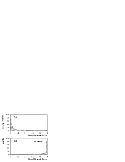
FIG. 24.: Initial training of the neural network (NN₀). The network output is shown for (a) data, and (b) herwig $t\bar{t}$ Monte Carlo for $m_{t}$=180 GeV/$c^{2}$.

Training of the two neural networks used in the final analysis proceeded as follows. The first neural network (NN₁) was trained on the ten kinematic variables using the training sets, as described above. The output of NN₁, and the remaining three variables were then used as inputs to the second neural network (NN₂). NN₂ was trained using tagged herwig $t\bar{t}$ Monte Carlo events and “fake” tagged data, also described in Sec. VII.D.

F Cross section using neural network fits

The $t\bar{t}$ cross section, integrated over all values of neural network output, is determined from the distributions in the output of the final neural network. Any excess of the tagged data over the modeled background distribution is attributed to $t\bar{t}$ production. This excess, integrated over all values of neural network output, is independent of the neural network, and depends only on the accuracy of the modeling of the background by the tag rate function. If the location of any excess appears in the region of $t\bar{t}$ signal (in neural network output) it would make these events likely $t\bar{t}$ candidates. The final neural network (NN₂) distributions for the data and the expected background are shown in Fig. 25(a), and for herwig $t\bar{t}$ events in Fig. 25(b). The normalization of the $t\bar{t}$ signal is described below. These distributions demonstrate a strong discrimination between signal and background.

FIG. 25.: The distributions in final neural network (NN₂) output for (a) data (diamonds) and expected background (histogram) and (b) herwig $t\bar{t}$ signal for $m_{t}$=180 GeV/$c^{2}$.

We extract the cross section from a fit to the data of the sum of the neural network output distributions expected for the $t\bar{t}$ signal and for QCD multijet background. Because the shapes of the $t\bar{t}$ and QCD network output distributions differ significantly, the relative amounts of each can be disentangled. The generated herwig $t\bar{t}$ events were arbitrarily normalized assuming $\sigma_{t\bar{t}}$ = 6.4 pb at each top quark mass. This value needs to be factored out in normalizing Fig. 25(b). The data of Fig. 25(a) are fitted using $\chi^{2}$ minimization to the hypothesis:

$$N_{\rm expected}={A_{\rm bkg}}~{}N^{i}_{\rm bkg}+\frac{\sigma_{t\bar{t}}}{6.4~{}{\rm pb}}~{}N^{i}_{t\bar{t}},$$ (25)

where $N^{i}_{\rm bkg}$ is the expected number of background events in the $i^{th}$ bin, and $N^{i}_{t\bar{t}}$ is the expected signal in this bin. Because the full Monte Carlo sample, scaled to the total number of events (given by 6.4 pb multiplied by the integrated luminosity), is subjected to exactly the same trigger and selection criteria as the data, $N^{i}_{t\bar{t}}$ accounts for the luminosity, branching ratio (BR), and $t\bar{t}$ efficiency of our selection criteria. Both $A_{\rm bkg}$, the background normalization factor, and $\sigma_{t\bar{t}}$, are obtained from the fit, along with their respective statistical errors. The results of this fit are shown in Fig. 26.

By allowing the signal and background normalization factors to be determined from the fit, this method simultaneously provides the $t\bar{t}$ cross section and a more sensitive measurement of the background normalization. It efficiently exploits all information about the $t\bar{t}$ cross section and background normalization from the entire range of neural network output, without choosing any particular cutoff on neural network output. The distributions for signal, background and data are shown separately in Fig. 26. The error bars are the square root of the number of data events in each bin.

Events at the lowest values of neural network output ($<0.02$) have been removed, leaving 2207 events, or slightly more than half of the tagged data sample. The resulting fits may be checked by varying the region of NN₂ used. (Fig. 26 uses events with NN${}_{2}>$ 0.02). Figure 27 shows results for $A_{\rm bkg}$ and $\sigma_{t\bar{t}}$ as a function of the lower limit in NN₂ employed in the fit. The results are seen to be quite stable to the change of this lower limit. We note that the jets in events with NN${}_{2}<$ 0.02 tend to have low $E_{T}$, where the tagging rate may not be as well determined due to the low tagging probability. Because the background modeling may be less accurate in the very low NN₂ region, where the background so strongly dominates the data distribution, we impose a cut of NN${}_{2}>$ 0.02 for our fits to $A_{\rm bkg}$ and $\sigma_{t\bar{t}}$. The stability of the results shown in Fig. 27 supports this choice.

FIG. 26.: The distribution in neural network (NN₂) output for data (diamonds) and the fits for expected signal and background. The signal was modeled with herwig for $m_{t}$=180 GeV/$c^{2}$. The errors shown are statistical.

A similar plot was produced and fitted for several top quark masses, and the values of the cross section obtained using the output distribution for herwig $t\bar{t}$ events generated at that mass. The results are shown in Table VI for several top quark masses. Interpolating to the value for the top quark mass as measured by DØ [5] ($m_{t}$ = 172.1 $\pm$ 7.1 GeV), we obtain $\sigma_{t\bar{t}}$ = 7.1 $\pm$ 2.8(stat) pb.

Fitting the data in Fig. 26 only to the background ($\sigma_{t\bar{t}}$ forced to zero), changes the normalization to 1.09 $\pm$ 0.03, and the total $\chi^{2}$ per degree-of-freedom to 23.1/18. We note that the change in $\chi^{2}$ comes predominantly from the last three bins of neural network output (in Fig. 26), and the probability for a change in $\chi^{2}$ of 6.2 (for $m_{t}$=180 GeV/$c^{2}$) for one additional degree-of-freedom is consistent with the significance of the extracted cross section, which is 2.5 standard deviations from zero.

FIG. 27.: Results of combined fits (as in Fig. 26) when data points are removed at small values of neural network output. The refitted (a) background normalization and (b) $t\bar{t}$ cross section are plotted as a function of the number of points eliminated. Error bars are statistical, but are correlated through the error matrix.

TABLE VI.: Results of the fits to neural network output.

Top Quark	$A_{\rm bkg}$	$\sigma_{t\bar{t}}$	$\chi^{2}$ / d.o.f.
Mass (GeV/$c^{2}$)		(pb)
140	1.05 $\pm$ 0.03	18.4 $\pm$ 7.8	17.6 / 17
160	1.06 $\pm$ 0.03	9.3 $\pm$ 3.8	17.2 / 17
170	1.07 $\pm$ 0.02	7.2 $\pm$ 3.0	17.1 / 17
180	1.07 $\pm$ 0.03	6.3 $\pm$ 2.5	16.9 / 17
200	1.07 $\pm$ 0.03	5.1 $\pm$ 2.0	16.8 / 17
220	1.07 $\pm$ 0.03	4.4 $\pm$ 1.7	16.7 / 17

G Cross section using counting method

The traditional method for extracting the $t\bar{t}$ cross section served as a useful check on the above procedure. We assumed an absolute normalization of the background as given by the tag rate function. Taking the excess in observed events (seen in Fig. 26) to be from $t\bar{t}$ production, we calculate the cross section for the process using the conventional relation:

$$\sigma_{t\bar{t}}=\frac{N_{\rm obs}-N_{\rm bkg}}{\epsilon\times BR\times{\cal{L}}}$$ (26)

where N_obs is the number of observed events with neural network output greater than some threshold, N_bkg is the corresponding number of expected background events, $\epsilon\times BR$ is the branching ratio (BR) times the efficiency ($\epsilon$) of the criteria used for selecting $t\bar{t}$ events, and ${\cal{L}}$ is the total integrated luminosity (110.3 $\pm$ 5.8 pb^-1). We use herwig as the model for calculating the value of $\epsilon\times BR$.

The number of events, as a function of the threshold placed on the output of the neural network, is shown in Fig. 28(a). The error bars are the square root of the number of events in each bin. The upper smooth curve in Fig. 28(a) represents the sum of the expected signal and background, and the lower curve is just the expected background. The statistical error in the cross section depends upon where the threshold is placed. A plot of the relative statistical error versus the threshold on the output of the neural network is shown in Fig. 28(b). The fractional error ${\cal E}$ is approximated by:

$${\cal E}=\frac{\sqrt{(N_{t\bar{t}}+N_{\rm bkg})}}{N_{t\bar{t}}},$$ (27)

where $N_{t\bar{t}}$ and $N_{\rm bkg}$ are the expected number of $t\bar{t}$ and background events above the neural network threshold. We wished to place the final threshold at or near the minimum error, and chose 0.85, as shown in Fig. 28(b). The number of events above this threshold, the expected background, and the expected signal are shown in Table VII.

FIG. 28.: (a) The number of events (data) above any threshold on the neural network, and (b) the expected fractional error on the $t\bar{t}$ cross section as a function of the threshold placed on the neural network output. The vertical line at 0.85 indicates the chosen threshold. The smooth curves in (a) represent the sum of the expected number of signal and background events (assuming $m_{t}$=180 GeV/$c^{2}$ and $\sigma_{t\bar{t}}$=6.4 pb) and the expected number of background events only.

TABLE VII.: Number of observed events, expected background, observed excess, and expected signal (assuming $m_{t}$=180 GeV/$c^{2}$ and $\sigma_{t\bar{t}}$=6.4 pb), for the threshold on the neural network output shown in Fig. 28.

Observed	Expected	Observed	Expected
Number	Background	Excess	herwig $t\bar{t}$
of Events	Events	of Events	Events
41	24.8$\pm$ 2.4	16.2	15.9 $\pm$ 2.6

Using Eq. 26, Table VIII lists the efficiency times branching ratios for two input top quark mass values, and the extracted $t\bar{t}$ cross sections. We note that the method in Sec. VII.F gave $t\bar{t}$ cross sections of 7.2 and 6.3 pb for $m_{t}$ of 170 and 180 GeV/$c^{2}$, respectively, in good agreement with the values in Table VIII. When interpolated to the measured top quark mass of 172.1 GeV/c², this determination yields a cross section of 7.3 $\pm$ 3.0 $\pm$ 1.6 pb. The results from the fit to the neural network are slightly lower, as one would expect, since the background normalization was 1.07 (instead of being fixed to 1 here). The changes in efficiencies as a function of top quark mass reflect the sensitivity of the selection criteria to the input mass $m_{t}$. The statistical and systematic uncertainties in the cross sections are discussed in Sec. VII.I.

TABLE VIII.: Cross sections for $t\bar{t}$ production, using the counting method, obtained from the $b$-tagged events for $m_{t}$ = 170 and 180 GeV/$c^{2}$.

$m_{t}$	Signal Efficiency	Cross Section
GeV/$c^{2}$	$\times$ BR	(pb)
170	0.019 $\pm$ 0.0032	7.5 $\pm$ 3.1 $\pm$ 1.6
180	0.022 $\pm$ 0.0037	6.5 $\pm$ 2.6 $\pm$ 1.4

H Double-tagged events

The requirement of a second $b$-tagged jet in the event further reduces the background, thereby increasing the signal-to-background ratio. Unfortunately, the additional requirement significantly reduces the expected yield. However, the search for these “double-tagged” events serves as a consistency check of the single-tag analysis, and also as a test of the model for the background. The number of events that contain two $b$-tagged jets is shown in Table IX for various NN₂ thresholds. The two $b$-tags are required to originate from separate jets; two tags within the same jet are counted as a single tag. The higher muon $p_{T}$ is used as the input to the neural network. The background is again calculated based on Eq. 21, where $P_{\rm tag}(E_{T},\eta,N_{\rm run})$, summed over all jets, represents the expected number of tags in the event. The double-tag probability is obtained via the Poisson distribution, and is the likelihood of observing at least two tagged jets, given the expected number. This follows since the tag rate function is a rate per jet, and, within our model, the two tagged jets are uncorrelated.

We make the assumption that the fraction of double-tagged events from correlated sources, such as direct heavy-quark pair production ($c\bar{c}$ or $b\bar{b}$), remains unchanged over the entire range of the neural network output variable. This assumption is motivated by the fact that the energy scales in such events are well above the energy thresholds for heavy-quark pair production, and therefore the fraction of these events should be independent of the neural network output. The good agreement between the background model and data in the single-tagged channel supports this assumption.

We determine the normalization of the background by fitting the neural network output distribution to the expected background and signal contributions as in Sec. VII.F. The 32 events were binned in neural network output, and the log-likelihood calculated. The minimum in negative log-likelihood occurs for a background normalization factor of 0.97${}^{+0.20}_{-0.18}$, where the errors correspond to a change in log-likelihood of 1/2. In determining this normalization, the expected $t\bar{t}$ signal was not varied, but the result is insensitive to this value. Allowing the data to determine the normalization through this fit accomodates the possibility that the tag rate function for the second muon in the event is different from that for the first muon. The two errors on the expected background in Table IX represent the uncertainties due to the tag rate function, $t\bar{t}$ subtraction and $E_{T}$ scale (see Sec. VII.I) and the normalization error, respectively.

We note that the fitted normalization is consistent with that for the single tagged sample indicating that the second muon tag probability is roughly the same as for the first. The total number of events for NN${}_{2}>0.02$ is in good agreement with the sum of expected background plus the small contribution from top. The small excess persists as the NN₂ threshold is increased, in agreement with expectations. The double tag analysis supports our conclusion that the singly-tagged sample is due to $t\bar{t}$ production.

TABLE IX.: Number of observed double-tagged events, expected background, observed excess, and expected signal (assuming $m_{t}$=180 GeV/$c^{2}$ and $\sigma_{t\bar{t}}$=6.4 pb), versus the threshold on the neural network output. The first error in the expected background is due to the errors in the tag rate function, $t\bar{t}$ correction, and the $E_{T}$ scale uncertainties. The second error is due to the uncertainty in the fitted background normalization factor, and is assumed to be fully correlated at different NN₂ values.

NN2	Observed	Expected	Observed	Expected
Threshold	Number	Background	Excess	herwig $t\bar{t}$
	of Events	Events	of Events	Events
0.02	32	28.7 $\pm$ 5.5 $\pm$ 5.7	3.3	2.7
0.1	22	16.6 $\pm$ 3.2 $\pm$ 3.3	5.4	2.7
0.2	17	11.8 $\pm$ 2.3 $\pm$ 2.3	5.2	2.7
0.4	12	6.8 $\pm$ 1.3 $\pm$ 1.4	5.2	2.5
0.6	7	3.5 $\pm$ 0.7 $\pm$ 0.7	3.5	2.1
0.8	3	1.1 $\pm$ 0.2 $\pm$ 0.2	1.9	1.4
0.85	2	0.7 $\pm$ 0.1 $\pm$ 0.1	1.3	1.2
0.9	1	0.4 $\pm$ 0.1 $\pm$ 0.1	0.6	1.0

I Corrections and uncertainties

In this subsection we discuss the major sources of systematic uncertainty that affect either the background estimate or signal efficiency. The statistical errors on the cross section and background normalization come directly from the fit (Eq. 25) shown in Fig. 26.

• The statistical error in the calculation of the background is estimated by the number of untagged events falling in the signal region. This estimate of 24.8 events, and an approximate mean tagging rate of 2%, implies of the order of 1240 untagged events for the background, and a consequent 3% statistical uncertainty in the background estimate. This contributes a 4% uncertainty in the cross section based on the counting method in Eq. 26.

• The error in the normalization of the tagging rate was taken from the combined fits to the output of the neural networks using Eq. 25. This error is shown in Fig. 27(a), and was taken to be 5%. It is used only in the calculation of the error on the background, as it is already included in the cross section. (The statistical error on the cross section was obtained from a simultaneous fit to the normalization of both background and signal, and accounts for the error on the background normalization.)

• The uncertainty in the parameterization of the tagging rate results in a 5% uncertainty in the predicted number of background events. This was estimated by comparing the predicted number of tags for two functional forms (Eq. 22 and Eq. 23) assumed for the tag rate. Unlike the normalization of the tagging rate, this error accounts for possible changes in the shape of the background as a function of neural network output. This results in a 7% uncertainty in the $t\bar{t}$ cross section.

• The presence of $t\bar{t}$ events in the data used for estimating background has been taken into account in all results presented thus far. The procedure used to estimate the correction to the background proceeds as follows. Calling $N_{t\bar{t}}^{\rm mistag}$ the number of untagged $t\bar{t}$ events wrongly assigned to the background estimate, we can estimate $N_{t\bar{t}}^{\rm mistag}$ as:

  $$N_{t\bar{t}}^{\rm mistag}=\frac{0.8}{0.2}(N_{\rm obs}-N_{\rm bkg})f_{\rm tag}$$ (28)

  where the $\frac{0.8}{0.2}$ corrects the $b$-tagged signal back to the untagged signal (recall that $t\bar{t}$ events are tagged roughly 20% of the time), $f_{\rm tag}$ is the average tag rate per event, and $N_{\rm obs}$ and $N_{\rm bkg}$ refer to events in the final tagged data sample. The corrected background estimation therefore becomes:

  $$N_{\rm bkg}(corr)=N_{\rm bkg}-N_{t\bar{t}}^{\rm mistag}$$ (29)

  This correction is applied bin by bin in Fig. 26, and is approximately 4% in the signal region. We therefore assign a systematic uncertainty of 4% to the background estimate and a corresponding 6% to the $t\bar{t}$ cross section.

• Because untagged events, when multiplied by the tag rate function, model the tagged background, the $E_{T}$ scale of both sets must be the same. Any mismatch between these can produce subtle differences in the scales of the kinematic variables. A useful measure of this scale is mean $H_{T}$. We observe that the difference in mean $H_{T}$ between our data and background model is 1.5 $\pm$ 1.4 GeV (see Fig. 23(a)), which is consistent with no mismatch. We take 1.4 GeV to be the uncertainty in the energy scale of the background model. This 1.4 GeV is added to one of the jets (we arbitrarily choose the jet with highest $E_{T}$), event-by-event, in the background calculation and the analysis is redone. The resultant change in the background is 4.2%, and 9.1% change in the cross section.

• The statistical error in the $t\bar{t}$ efficiency is 3.2%.

• Any difference in the turn-on of the trigger efficiency for data and for $t\bar{t}$ Monte Carlo events can affect the signal efficiency. The difference can originate, for example, from the modeling of electronic noise or from the simulation of the underlying event. Furthermore, this efficiency can depend upon the mass of the top quark. From our trigger simulations, we estimate $<$ 5% uncertainty in signal efficiency from such sources [12, 13].

• The uncertainty in the integrated luminosity was taken to be 5.3% [32]. This arises mainly from the uncertainty in the absolute luminosity, and affects all runs systematically.

• Any difference in the relative energy scale between data and Monte Carlo affects the efficiency for signal. This uncertainty was determined using the MPF method[17], as described in Sec. IV.C. Varying the energy scale in the $t\bar{t}$ Monte Carlo by $\pm$ (4% + 1 GeV) [6] changes the efficiency for signal by $\pm$ 5.7%.

• The $t\bar{t}$ tag rate is based on the $t\bar{t}$ Monte Carlo, but assumes that the performance of all detector components was stable during the run. The Monte Carlo acceptance was reduced by 7.0% to correct mainly for muon detection inefficiencies that were not modeled in our simulation. We estimate a 7.0% uncertainty in the $t\bar{t}$ efficiency from any such changes in the muon tag rate.

• Uncertainty in the model for $t\bar{t}$ production is estimated by comparing $t\bar{t}$ predictions from isajet and herwig generators. Figure 29 shows the fractional differences in efficiencies (($\epsilon_{\sc isajet}$ - $\epsilon_{\sc herwig}$)/$\epsilon_{\sc herwig}$) for different thresholds on $H_{T}$, $H_{T}^{3j}$, Aplanarity and $\cal{C}$ (again, for $m_{t}$ = 180 GeV/$c^{2}$). Although the two generators differ significantly in the tails of these distributions, on average they are in reasonable agreement. The systematic error was estimated by repeating the analysis using events generated with isajet. In order to remove the effects of the Fisher discriminant (${\cal F}$), which is not well modeled in isajet, ${\cal F}$ values were randomly chosen based on a parameterization of the herwig $t\bar{t}$ ${\cal F}$ distribution. To further remove the dependence on the tag rate, randomly generated values of muon $p_{T}$ were taken. The expected distributions for the two generators, normalized as before, are shown in Fig. 30. Identical thresholds were placed on the neural network output. The cross section changed by 6.2%, which we take as the uncertainty in the overall signal efficiency due to $t\bar{t}$ model dependence.

  

  FIG. 29.: Fractional differences in efficiencies between isajet and herwig ($\epsilon_{\sc isajet}$ - $\epsilon_{\sc herwig}$)/$\epsilon_{\sc herwig}$ for $m_{t}$ = 180 GeV/$c^{2}$ (a) as a function of threshold on $H_{T}$, (b) as a function of threshold on $H_{T}^{3j}$, (c) as a function of threshold on Aplanarity, and (d) as a function of threshold on $\cal{C}$.

  

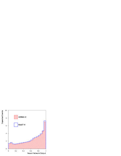
  FIG. 30.: Expected distributions in final neural network output (NN₂) for herwig $t\bar{t}$ signal and isajet $t\bar{t}$ signal for $m_{t}$=180 GeV/$c^{2}$.

• The 6% uncertainty in the $b\rightarrow\mu$ branching fraction [28] corresponds to an average over the produced $B$-mesons. This 6% enters directly into the acceptance error in the Monte Carlo.

• The $p_{T}$ of the tagged muon enters as an input to the neural network. The mean $p_{T}$ in herwig $t\bar{t}$ events was 14.7 GeV/$c$, while in isajet it was 15.9 GeV/$c$, an 8% difference. Rescaling the muon $p_{T}$ in herwig by 8% changes the cross section by 7.0%, which is taken as a systematic error.

• The uncertainty resulting from the modeling of the Fisher discriminant for the jet widths, ${\cal F}$, was estimated by comparing data to our herwig QCD Monte Carlo. The mean value of ${\cal F}$ in data was 0.0470 $\pm$ 0.0002 and in herwig QCD it was 0.0488 $\pm$ 0.0019. The difference of 0.0018 $\pm$ 0.0019 indicates that our modeling is reasonable. The uncertainty on this result, 0.0019, was systematically added to the value of ${\cal F}$, event-by-event, in the herwig $t\bar{t}$ generator, and the cross section recalculated. The observed change in the cross section of 2.0% is used as the systematic error from this variable.

  TABLE X.: Summary of statistical and systematic uncertainties for the background estimate.

  Background Source	Size of Uncertainty
  Statistical Error	3 %
  Normalization of the Muon Tag Rate	5 %
  Functional Form of the Muon Tag Rate	5 %
  Background Correction for $t\bar{t}$ Signal	4 %
  Background $E_{T}$ Scale	4 %

  TABLE XI.: Summary of statistical and systematic uncertainties for the cross section.

  Background Source	Size of Uncertainty
  Statistical error	4 %
  Functional Form of the Muon Tag Rate	7 %
  Background Correction for $t\bar{t}$ Signal	6 %
  Background $E_{T}$ scale	9 %
  Signal Source	Size of Uncertainty
  Statistical Error	3 %
  Trigger Turn-on	5 %
  Luminosity Error	5 %
  Jet Energy Scale	6 %
  $t\bar{t}$ Tag Rate	7 %
  Model Dependence	6 %
  $b\rightarrow\mu$ Branching Fraction	6 %
  $p_{T}^{\mu}$ Dependence	7 %
  ${\cal{F}}$ Dependence	2 %

The sizes of the above effects are summarized in Table X for the uncertainties in the background, and in Table XI for the cross section. Adding both statistical and systematic errors in quadrature, we estimate the background as 24.8 $\pm$ 2.4 events (see Table VII). Similarly, the uncertainty in the efficiency of the $t\bar{t}$ signal is calculated from the errors in Table XI.

J Measured cross section

By fitting the shape of the output in the neural network distribution, we obtain the $t\bar{t}$ production cross section as a function of the input mass of the top quark. The $t\bar{t}$ cross sections extracted for several values of the top quark mass, along with a function used to interpolate the $t\bar{t}$ cross section (drawn as a smooth curve), are shown in Fig. 31. Interpolating both the cross section and the statistical error, we find $\sigma_{t\bar{t}}$ = 7.1 $\pm$ 2.8 $\pm$ 1.5 pb for $m_{t}$=172.1 GeV/$c^{2}$ [5].

The all-jets cross section can be combined with previous DØ measurements of the $t\bar{t}$ production cross section, as extracted from channels where one or both of the $W$ bosons decay leptonically [6]. This cross section, averaged over all leptonic channels, was 5.6 $\pm$ 1.4 (stat) $\pm$ 1.2 (syst) pb at $m_{t}$=172.1 GeV/$c^{2}$, and is shown superimposed on Fig. 31. The statistical errors on the all-jets and leptonic cross section measurements are uncorrelated. The systematic uncertainties in the following categories were assumed to be correlated with a correlation coefficient of 1.0.

• Luminosity.

• Jet energy scale.

• Muon tagging efficiency.

• Non-leptonic trigger efficiency.

• Top quark generator.

• $b\rightarrow\mu$ branching ratio and muon $p_{T}$ spectrum.

• Background tag rate function.

The combined result for the DØ $t\bar{t}$ production cross section is 5.9 $\pm$ 1.2 (stat) $\pm$ 1.1 (syst) pb for $m_{t}$=172.1 GeV/$c^{2}$.

K Significance of signal

In this section, we estimate the significance of the excess of $t\bar{t}$ signal relative to expected background. We define the probability ($P$) of seeing at least the number of observed events ($N_{\rm obs}$), when only background is expected. The significance of a $t\bar{t}$ signal can be characterized by the likelihood of $P$ being due to a fluctuation. If the distribution for the expected number of background events, $\mu$, is assumed to be a Gaussian with mean $b$, and has a systematic uncertainty $\sigma_{b}$, then $P$ can be calculated as:

$$P = \sum_{n=N_{\rm obs}}^{\infty}\int^{\infty}_{0}d\mu\frac{e^{-\mu}\mu^{n}}{n!}\frac{1}{\sqrt{2\pi}\sigma_{b}}e^{-(\mu-b)^{2}/2\sigma_{b}^{2}}$$ (30)

$$= 1-\sum_{n=0}^{N_{\rm obs}-1}\int^{\infty}_{0}d\mu\frac{e^{-\mu}\mu^{n}}{n!}\frac{1}{\sqrt{2\pi}\sigma_{b}}e^{-(\mu-b)^{2}/2\sigma_{b}^{2}}$$ (31)

The optimal choice of selection criteria can be found by minimizing the expected value of $P$ and, thereby, maximizing the significance of the excess, assuming that $N_{\rm obs}$ is composed of $t\bar{t}$ signal and background. Both the expected value and measured value of the significance are shown, along with the cutoff for greatest significance, in Fig. 32. The result of the calculation, optimized for significance, with 18 observed events and an expected background of 6.9 $\pm$ 0.9, is $P$ = 0.0006, corresponding to a 3.2 standard deviation effect. This is sufficient to establish the existence of a $t\bar{t}$ signal in multijet final states.

FIG. 31.: The $t\bar{t}$ cross section extracted through fitting the shapes of the distributions in neural network output to data, shown as a function of top quark mass. Error bars are statistical only. For reference, the DØ $t\bar{t}$ cross section and top quark mass from leptonic channels [6] is shown in the figure (open square).

FIG. 32.: The expected (line) and observed (diamonds) values of significance of $t\bar{t}$ signal, plotted in terms of Gaussian equivalent standard deviations. The vertical line corresponds to the cutoff that is expected to yield the greatest significance.

We consequently observe an excess in the multijet final states which we attribute to $t\bar{t}$ production. The cross section measured is consistent with previous measurements in other modes of $t\bar{t}$ decay[6].

VIII Summary

We have performed a measurement of the $t\bar{t}$ production cross section in multijet final states. As described above, we observe an excess of events that can be attributed to $t\bar{t}$ production. The level of significance of the signal, as calculated from a possible upward fluctuation of the background to produce the observed excess, is sufficiently high to establish independently the existence of $t\bar{t}$ signal in the all-jets channel.

Using the DØ measured value of 172.1 GeV/$c^{2}$ for the mass of the top quark, we obtain a cross section of 7.1 $\pm$ 2.8 (stat) $\pm$ 1.5 (syst) pb, which agrees with the DØ cross section as measured in the leptonic channels. Combining this result with previous DØ measurements of the $t\bar{t}$ production cross section gives 5.9 $\pm$ 1.2 (stat) $\pm$ 1.1 (syst) pb.

REFERENCES

- [1] Visitor from Universidad San Francisco de Quito, Quito, Ecuador.
- [2] Visitor from IHEP, Beijing, China.
- [3] DØ Collaboration, S. Abachi et al., Phys. Rev. Lett. 74, 2632 (1995).
- [4] CDF Collaboration, F. Abe et al., Phys. Rev. Lett. 74, 2626 (1995).
- [5] DØ Collaboration, B. Abbott et al., to be published in Phys. Rev. D, FERMILAB-Pub-98/031-E, (1998).
- [6] DØ Collaboration, S. Abachi et al., Phys. Rev. Lett. 79, 1203 (1997).
- [7] CDF Collaboration, F. Abe et al., Phys. Rev. Lett. 80, 2767 (1998).
- [8] CDF Collaboration, F. Abe et al., Phys. Rev. Lett. 80, 2779 (1998).
- [9] CDF Collaboration, F. Abe et al., Phys. Rev. Lett. 79, 1992 (1997).
- [10] DØ Collaboration, S. Abachi et al., Nucl. Instr. Methods Phys. Res. A 338, 185 (1994).
- [11] DØ Collaboration, S. Abachi et al., Phys. Rev. D 52, 4877 (1995).
- [12] C. Cretsinger, Ph.D. thesis, University of Rochester, 1995, (unpublished), available from http://www-d0.fnal.gov/publications_talks/ thesis/cretsinger/thesis_final.ps.
- [13] E. Won, Ph.D. thesis, University of Rochester, 1996, (unpublished), available from http://www-d0.fnal.gov/publications_talks/ thesis/won/thesis.ps.
-
[14]
UA1 Collaboration, G. Arnison et al., Phys. Lett.
123B, 115 (1983).
B. Abbott et al., FERMILAB-Pub-97/242-E, unpublished. - [15] G. Marchesini et al., Comput. Phys. Commun. 67, 465 (1992).
-
[16]
DØ Collaboration, R. Kehoe, in Proceedings of the
Sixth International Conference on Calorimetry in High
Energy Physics, Frascati, Italy (World Scientific, River
Edge, NJ, 1996), FERMILAB-Conf-96/284-E.
DØ Collaboration, B. Abbott et al., submitted to Nucl. Instr. and Methods Res. A, FERMILAB-Pub-97/330-E, (1998). - [17] CDF Collaboration, F. Abe et al., Phys. Rev. Lett. 69, 2896 (1992).
- [18] F. Paige and S. Protopopescu, BNL Report no. BNL38034, 1986 (unpublished), release v6.49.
- [19] R. Raja, Proceedings of the Workshop on Detector Simulation for the SSC, Argonne, 1987, Fermilab-Conf-88/16-E.
- [20] The geant Manual, F. Carminati et al., CERN Geneva (1996), Unpublished.
- [21] DØ Collaboration, S. Abachi et al., Nucl. Instr. Methods Phys. Res. A 324, 53 (1993).
- [22] V.D. Barger and R.J.N. Phillips, Collider Physics (Addison-Wesley, Massachusetts, 1987).
- [23] AMY Collaboration, Y.K. Kim et al., Phys. Rev. Lett. 63, 1772 (1989).
-
[24]
OPAL Collaboration, G. Alexander et al.,
Phys. Lett. B 265, 462 (1991).
OPAL Collaboration, G. Alexander et al., Z.Phys. C68, 179 (1995). - [25] DØ Collaboration, S. Abachi et al., Phys. Lett. B 357, 500 (1995).
- [26] B. Abbott, Ph.D. thesis, Purdue University, 1994, (unpublished), available from http://www-d0.fnal.gov/publications_talks /thesis/abbott/ thesis_abbott.
- [27] P. R. Bevington, Data Reduction and Error Analysis for the Physical Sciences (McGraw-Hill, New York, 1969).
- [28] Particle Data Group, Phys. Rev. D 54, (1996).
- [29] H. Xu, Ph.D. thesis, Brown University, 1995, (unpublished), available from http://www-d0.fnal.gov/publications_talks /thesis/ Xu/thesis.ps.
-
[30]
P. Bhat, hep-ex/9507007 (1995), unpublished.
R. Beale and T. Jackson, Neural Computing: An Introduction (Adam Hilger, New York, 1991).
J. Hertz, A. Krogh, and R. G. Palmer, Introduction to the Theory of Neural Computation, (Addison-Wesley, Massachusetts, 1990). - [31] C. Peterson and T. Rgnvaldsson, JETNET 3.0 - A Versatile Artifical Neural Network Package, CERN-TH.7135/94 (1994).
- [32] J. Bantly et al., FERMILAB-TM-1995, (1997), unpublished.