Observation of $B^{+}\rightarrow\omega K^{+}$
and Search for Related $B$ Decay Modes.

Abstract

We have searched for two-body charmless decays of $B$ mesons to purely hadronic exclusive final states including $\omega$ or $\phi$ mesons using data collected with the CLEO II detector. With this sample of $6.6\times 10^{6}$ $B$ mesons we observe a signal for the $\omega K^{+}$ final state, and measure a branching fraction of ${\cal B}(B^{+}\rightarrow\omega K^{+})=(1.5^{+0.7}_{-0.6}\pm 0.2)\times 10^{-5}$. We also observe some evidence for the $\phi K^{*}$ final state, and upper limits are given for 22 other decay modes. These results provide the opportunity for studies of theoretical models and physical parameters.

T. Bergfeld,¹ B. I. Eisenstein,¹ J. Ernst,¹ G. E. Gladding,¹ G. D. Gollin,¹ R. M. Hans,¹ E. Johnson,¹ I. Karliner,¹ M. A. Marsh,¹ M. Palmer,¹ M. Selen,¹ J. J. Thaler,¹ K. W. Edwards,² A. Bellerive,³ R. Janicek,³ D. B. MacFarlane,³ P. M. Patel,³ A. J. Sadoff,⁴ R. Ammar,⁵ P. Baringer,⁵ A. Bean,⁵ D. Besson,⁵ D. Coppage,⁵ C. Darling,⁵ R. Davis,⁵ S. Kotov,⁵ I. Kravchenko,⁵ N. Kwak,⁵ L. Zhou,⁵ S. Anderson,⁶ Y. Kubota,⁶ S. J. Lee,⁶ J. J. O’Neill,⁶ R. Poling,⁶ T. Riehle,⁶ A. Smith,⁶ M. S. Alam,⁷ S. B. Athar,⁷ Z. Ling,⁷ A. H. Mahmood,⁷ S. Timm,⁷ F. Wappler,⁷ A. Anastassov,⁸ J. E. Duboscq,⁸ D. Fujino,^8, K. K. Gan,⁸ T. Hart,⁸ K. Honscheid,⁸ H. Kagan,⁸ R. Kass,⁸ J. Lee,⁸ M. B. Spencer,⁸ M. Sung,⁸ A. Undrus,^8, A. Wolf,⁸ M. M. Zoeller,⁸ B. Nemati,⁹ S. J. Richichi,⁹ W. R. Ross,⁹ H. Severini,⁹ P. Skubic,⁹ M. Bishai,¹⁰ J. Fast,¹⁰ J. W. Hinson,¹⁰ N. Menon,¹⁰ D. H. Miller,¹⁰ E. I. Shibata,¹⁰ I. P. J. Shipsey,¹⁰ M. Yurko,¹⁰ S. Glenn,¹¹ Y. Kwon,^11, A.L. Lyon,¹¹ S. Roberts,¹¹ E. H. Thorndike,¹¹ C. P. Jessop,¹² K. Lingel,¹² H. Marsiske,¹² M. L. Perl,¹² V. Savinov,¹² D. Ugolini,¹² X. Zhou,¹² T. E. Coan,¹³ V. Fadeyev,¹³ I. Korolkov,¹³ Y. Maravin,¹³ I. Narsky,¹³ V. Shelkov,¹³ J. Staeck,¹³ R. Stroynowski,¹³ I. Volobouev,¹³ J. Ye,¹³ M. Artuso,¹⁴ F. Azfar,¹⁴ A. Efimov,¹⁴ M. Goldberg,¹⁴ D. He,¹⁴ S. Kopp,¹⁴ G. C. Moneti,¹⁴ R. Mountain,¹⁴ S. Schuh,¹⁴ T. Skwarnicki,¹⁴ S. Stone,¹⁴ G. Viehhauser,¹⁴ J.C. Wang,¹⁴ X. Xing,¹⁴ J. Bartelt,¹⁵ S. E. Csorna,¹⁵ V. Jain,^15, K. W. McLean,¹⁵ S. Marka,¹⁵ R. Godang,¹⁶ K. Kinoshita,¹⁶ I. C. Lai,¹⁶ P. Pomianowski,¹⁶ S. Schrenk,¹⁶ G. Bonvicini,¹⁷ D. Cinabro,¹⁷ R. Greene,¹⁷ L. P. Perera,¹⁷ G. J. Zhou,¹⁷ M. Chadha,¹⁸ S. Chan,¹⁸ G. Eigen,¹⁸ J. S. Miller,¹⁸ M. Schmidtler,¹⁸ J. Urheim,¹⁸ A. J. Weinstein,¹⁸ F. Würthwein,¹⁸ D. W. Bliss,¹⁹ G. Masek,¹⁹ H. P. Paar,¹⁹ S. Prell,¹⁹ V. Sharma,¹⁹ D. M. Asner,²⁰ J. Gronberg,²⁰ T. S. Hill,²⁰ D. J. Lange,²⁰ R. J. Morrison,²⁰ H. N. Nelson,²⁰ T. K. Nelson,²⁰ D. Roberts,²⁰ B. H. Behrens,²¹ W. T. Ford,²¹ A. Gritsan,²¹ H. Krieg,²¹ J. Roy,²¹ J. G. Smith,²¹ J. P. Alexander,²² R. Baker,²² C. Bebek,²² B. E. Berger,²² K. Berkelman,²² K. Bloom,²² V. Boisvert,²² D. G. Cassel,²² D. S. Crowcroft,²² M. Dickson,²² S. von Dombrowski,²² P. S. Drell,²² K. M. Ecklund,²² R. Ehrlich,²² A. D. Foland,²² P. Gaidarev,²² L. Gibbons,²² B. Gittelman,²² S. W. Gray,²² D. L. Hartill,²² B. K. Heltsley,²² P. I. Hopman,²² J. Kandaswamy,²² P. C. Kim,²² D. L. Kreinick,²² T. Lee,²² Y. Liu,²² N. B. Mistry,²² C. R. Ng,²² E. Nordberg,²² M. Ogg,^22, J. R. Patterson,²² D. Peterson,²² D. Riley,²² A. Soffer,²² B. Valant-Spaight,²² C. Ward,²² M. Athanas,²³ P. Avery,²³ C. D. Jones,²³ M. Lohner,²³ S. Patton,²³ C. Prescott,²³ J. Yelton,²³ J. Zheng,²³ G. Brandenburg,²⁴ R. A. Briere,²⁴ A. Ershov,²⁴ Y. S. Gao,²⁴ D. Y.-J. Kim,²⁴ R. Wilson,²⁴ H. Yamamoto,²⁴ T. E. Browder,²⁵ Y. Li,²⁵ and J. L. Rodriguez²⁵

In the last several years, the study of charmless non-leptonic decays of $B$ mesons has attracted a lot of attention, primarily because of the importance of these processes in understanding the phenomenon of $CP$ violation. This interest is expected to continue as several new experimental facilities specifically built for $B$ meson studies begin operating within a few years. Purely hadronic decays of $B$ mesons are understood to proceed mainly through the weak decay of a $b$ quark to a lighter quark, while the light quark bound in the $B$ meson remains a spectator, as shown by the Feynman diagrams in Figure 1. The decay amplitude for “tree-level” $b\rightarrow u$ transitions (Figure 1(a) and (b)) is much smaller than the one for dominant $b\rightarrow c$ transitions due to the ratio of Cabibbo-Kobayashi-Maskawa [1] matrix elements $V_{ub}/V_{cb}\approx 0.1$. Transitions to $s$ and $d$ quarks are effective flavor-changing neutral currents proceeding mainly by one-loop “penguin” amplitudes, and are also suppressed. Examples are shown in Figure 1 (c) and (d).

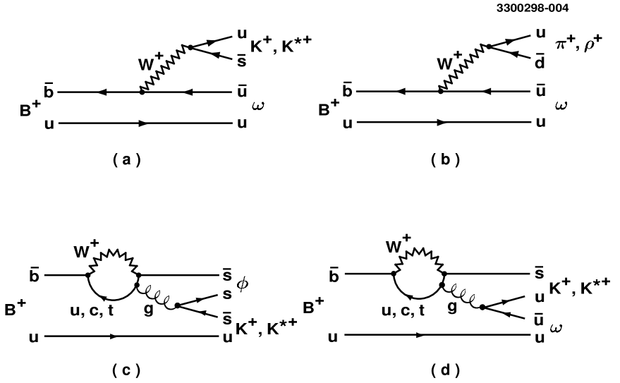
FIG. 1.: (a) and (b) tree-level spectator and (c) and (d) penguin diagrams for some of the decay modes investigated.

The strong interaction between particles in the final state makes theoretical predictions difficult. The use of effective hamiltonians, often with factorization assumptions [2, 3, 4, 5, 6, 7, 8, 9, 10], has led to a number of these predictions, and the experimental sensitivity has now become sufficient to allow us to begin to test the correctness of the underlying assumptions [11, 12, 13].

In this letter, we describe searches for $B$-meson decays to exclusive final states that include an $\omega$ or $\phi$ meson and one other low-mass charmless meson. Some decays to final states with a $\phi$ are of particular interest because they are dominated by penguin amplitudes, and receive no contribution from tree-level amplitudes (see Figure 1), while others, such as $B^{+}\rightarrow\phi\pi^{+}$, receive no contribution from penguin or tree amplitudes and only proceed through higher-order diagrams.

The results presented here are based on data collected with the CLEO II detector [14] at the Cornell Electron Storage Ring (CESR). The data sample corresponds to an integrated luminosity of 3.11 fb^-1 for the reaction $e^{+}e^{-}\rightarrow\Upsilon(4S)\rightarrow B\overline{B}$, which in turn corresponds to $3.3\times 10^{6}$ $B\overline{B}$ pairs. To study background from continuum processes, we also collected 1.61 fb^-1 of data at a center-of-mass energy below the threshold for $B\overline{B}$ production.

The final states of the decays under study are reconstructed by combining detected photons and charged pions and kaons. The $\omega$ and $\phi$ mesons are identified via the decay modes $\omega\rightarrow\pi^{+}\pi^{-}\pi^{0}$ and $\phi\rightarrow K^{+}K^{-}$, respectively. The detector elements most important for the analyses presented here are the tracking system, which consists of 67 concentric drift chamber layers, and the high-resolution electromagnetic calorimeter, made of 7800 CsI(Tl) crystals.

Reconstructed charged tracks are required to pass quality cuts based on their track fit residuals and impact parameter. The specific ionization ($dE/dx$) measured in the drift layers is used to distinguish kaons from pions. Expressed as the number of standard deviations from the expected value, $S_{i}$($i=\pi,K$), it is required to satisfy $|S_{i}|<3.0$. Photons are defined as isolated showers, not matched to any charged tracks, with a lateral shape consistent with that of photons, and with a measured energy of at least 30 (50) MeV in the calorimeter region $|\cos{\theta}|<0.71(\geq 0.71)$, where $\theta$ is the polar angle.

Pairs of photons (charged pions) are used to reconstruct $\pi^{0}$’s and $\eta$’s ($K^{0}$’s). The momentum of the pair is obtained with a kinematic fit of the decay particle momenta with the meson mass constrained to its nominal value. To reduce combinatoric background, we reject very asymmetric $\pi^{0}$ and $\eta$ decays by requiring that the rest frame angle $\theta^{*}$ between the direction of the meson and the direction of the photons satisfy $|\cos{\theta^{*}}|<0.97$, and require that the momentum of charged tracks and photon pairs be greater than 100 MeV/$c$.

The primary means of identification of $B$ meson candidates is through their measured mass and energy. The quantity $\Delta E$ is defined as $\Delta E\equiv E_{1}+E_{2}-E_{b}$, where $E_{1}$ and $E_{2}$ are the energies of the two daughter particles of the $B$ and $E_{b}$ is the beam energy. The beam-constrained mass of the candidate is defined as $M\equiv\sqrt{E_{b}^{2}-|{\bf p}|^{2}}$, where $\bf p$ is the measured momentum of the candidate. We use the beam energy instead of the measured energy of the $B$ candidate to improve the mass resolution by about one order of magnitude.

The large background from continuum quark–antiquark ($q\bar{q}$) production can be reduced with event shape cuts. Because $B$ mesons are produced almost at rest, the decay products of the $B\bar{B}$ pair tend to be isotropically distributed, while particles from $q\bar{q}$ production have a more jet-like distribution. The angle $\theta_{T}$ between the thrust axis of the charged particles and photons forming the candidate $B$ and the thrust axis of the remainder of the event is required to satisfy $|\cos{\theta_{T}}|<0.9$. Continuum background is strongly peaked near 1.0 and signal is approximately flat for this quantity. We also form a Fisher discriminant (${\cal F}$) [11] with the momentum scalar sum of charged particles and photons in nine cones of increasing polar angle around the thrust axis of the candidate and the angles of the thrust axis of the candidate and $\bf p$ with respect to the beam axis.

The specific final states investigated are identified via the reconstructed invariant masses of the $B$ daughter resonances. For final states with a pseudoscalar meson, and for the secondary decay $\eta^{\prime}\rightarrow\rho\gamma$, further separation of signal events from combinatoric background is obtained through the use of the defined angular helicity state of the $\phi$, $\omega$, or $\rho$. The observable $\cal H$ is the cosine of the angle between the flight direction of the vector meson and the daughter decay direction (normal to the decay plane for the $\omega$), boosted to the meson’s rest frame. For the final states $\omega K^{*+}$ and $\omega\rho^{+}$, the $\pi^{0}$ from $K^{*+}$ or $\rho^{+}$ decay defines the daughter direction. In this case we require ${\cal H}<0.5$ to reduce the large combinatoric background from soft $\pi^{0}$’s. Since the distribution of $\cal H$ is not known for these vector-vector final states we assume the worst case (${\cal H}^{2}$) when computing the efficiency.

Signal event yields for each mode are obtained with unbinned multi-variable maximum likelihood fits. We also performed event counting analyses that applied tight constraints on all variables described above. Results for the latter are consistent with the ones presented below.

For $N$ input events and $p$ input variables, the likelihood is defined as

$${\cal L} = e^{-(N_{S}+N_{B})}\prod_{i=1}^{N}\{N_{S}\prod_{j=1}^{p}{\cal P}_{S_{ij}}(f_{1j},...,f_{mj};x_{ij})+$$

$$N_{B}\prod_{j=1}^{p}{\cal P}_{B_{ij}}(g_{1j},...,g_{nj};x_{ij})\},$$

where ${\cal P}_{S_{ij}}$ and ${\cal P}_{B_{ij}}$ are the probabilities for event $i$ to be signal and continuum background for variable $x_{ij}$, respectively. The probabilities are also a function of the parameters $f$ and $g$ used to describe the signal and background shapes for each variable. The number of parameters required varies depending on the input variable. The variables used are $\Delta E$, $M$, ${\cal F}$, resonance masses, and ${\cal H}$ as appropriate. For pairs of final states differentiated only by the identity of a single charged pion or kaon, we also use $S_{i}$ for that track and fit both modes simultaneously. $N_{S}$ and $N_{B}$, the free parameters of the fit, are the number of signal and continuum background events in the fitted sample, respectively. We verified that background from other $B$ decay modes is small for all channels investigated and did not require inclusion in the fit. Correlations between input variables were found to be negligible, except between the invariant masses of a parent resonance and its daughter, which the likelihood function takes into account.

For each decay mode investigated, the signal probability distribution functions (PDFs) for the input variables are determined with fits to Monte Carlo event samples generated with a GEANT [15] based simulation of the CLEO detector response. The parameters of the background PDFs are determined with similar fits to a sideband region of data defined by $|\Delta E|<0.2$ GeV and $5.2<M<5.27$ GeV/c². The data samples collected on and below the $\Upsilon(4S)$ resonance are used. The signal shapes used are Gaussian, double Gaussian, and Breit-Wigner as appropriate for $\Delta E$ and mass peaks. For background, resonance masses are fit to the sum of a smooth polynomial and the signal shape, to account for the component of real resonance as well as the combinatoric background. For $\Delta E$ and $M$ background we use a first-degree polynomial and the empirical shape $f(z)\propto M\sqrt{1-z^{2}}\exp{(-\xi(1-z^{2}))}$, where $z\equiv M/E_{b}$ and $\xi$ is a parameter to be fit, respectively. Finally, for ${\cal F}$, $S_{K}$, and $S_{\pi}$, we use bifurcated Gaussians for both signal and background.

Sideband regions for each input variable are included in the likelihood fit. The number of events input to the fit varies from 70 to $\sim 12000$, depending on the final state. Table I [16] gives the results for each mode investigated. The final state $\omega h^{+}$ represents the sum of the $\omega K^{+}$ and $\omega\pi^{+}$ states ($h^{+}\equiv K^{+}$ or $\pi^{+}$). Shown are the signal event yield, the efficiency, the product of the efficiency and the relevant branching fractions of particles in the final state, and the branching fraction for each mode, given as a central value with statistical and systematic error, or as a 90% confidence level upper limit. The one standard deviation ($\sigma$) statistical error is determined by finding the values where the quantity $\chi^{2}=-2\ln({\cal L}/{\cal L}_{\rm max})$, where ${\cal L}_{\rm max}$ is the point of maximum likelihood, changes by one unit.

TABLE I.: Measurement results. Columns list the final states (with secondary decay modes as subscripts), event yield from the fit, reconstruction efficiency $\epsilon$, total efficiency including secondary branching fractions ${\cal B}_{s}$, and the resulting $B$ decay branching fraction ${\cal B}$.

Final state	Yield(events)	$\epsilon$(%)	$\epsilon\mbox{${\cal B}$}_{s}$(%)	${\cal B}$($10^{-5})$
$\omega K^{+}$	$12.2^{+5.5}_{-4.5}$	28	25.1	$1.5^{+0.7}_{-0.6}\pm 0.2$
$\omega K^{0}$	$2.3^{+2.4}_{-1.5}$	15	4.4	$<5.7$
$\omega\pi^{+}$	$9.2^{+5.3}_{-4.3}$	29	25.8	$<2.3$
$\omega h^{+}$	$21.4^{+6.5}_{-5.6}$	29	25.5	$2.5^{+0.8}_{-0.7}\pm 0.3$
$\omega\pi^{0}$	$2.4^{+2.9}_{-1.8}$	24	20.9	$<1.4$
$\omega{\eta^{\prime}}_{\eta\pi\pi}$	$0.1^{+1.9}_{-0.1}$	16	2.4	$<6.4$
$\omega{\eta^{\prime}}_{\rho\gamma}$	$5.1^{+3.6}_{-2.7}$	16	4.2	$<9.2$
$\omega\eta_{{\gamma\gamma}}$	$0.0^{+1.5}_{-0.0}$	24	8.5	$<2.0$
$\omega\eta_{3\pi}$	$0.0^{+0.5}_{-0.0}$	15	3.2	$<2.8$
$\omega K^{*+}_{K^{+}\pi^{0}}$	$1.1^{+2.6}_{-1.1}$	7	2.0	$<12.9$
$\omega K^{*+}_{K^{0}\pi^{+}}$	$4.5^{+3.6}_{-2.8}$	16	3.2	$<10.9$
$\omega K^{*0}_{K^{+}\pi^{-}}$	$2.1^{+3.6}_{-2.1}$	22	13.1	$<2.3$
$\omega\rho^{+}$	$2.5^{+4.4}_{-2.5}$	8	6.8	$<6.1$
$\omega\rho^{0}$	$0.0^{+1.7}_{-0.0}$	24	21.1	$<1.1$
$\omega\omega$	$0.3^{+2.6}_{-0.3}$	15	11.9	$<1.9$
$\phi K^{+}$	$0.0^{+0.8}_{-0.0}$	47	23.1	$<0.5$
$\phi K^{0}$	$1.9^{+2.0}_{-1.2}$	32	5.3	$<3.1$
$\phi\pi^{+}$	$0.0^{+0.9}_{-0.0}$	49	24.0	$<0.5$
$\phi\pi^{0}$	$0.0^{+0.6}_{-0.0}$	31	15.1	$<0.5$
$\phi{\eta^{\prime}}_{\eta\pi\pi}$	$0.0^{+0.5}_{-0.0}$	26	2.2	$<3.5$
$\phi{\eta^{\prime}}_{\rho\gamma}$	$2.7^{+3.1}_{-2.1}$	30	4.4	$<6.3$
$\phi\eta_{{\gamma\gamma}}$	$0.0^{+0.6}_{-0.0}$	39	7.5	$<1.3$
$\phi\eta_{3\pi}$	$0.0^{+0.5}_{-0.0}$	24	2.7	$<2.9$
$\phi K^{*+}_{K^{+}\pi^{0}}$	$2.6^{+3.3}_{-2.4}$	26	4.4	$<5.6$
$\phi K^{*+}_{K^{0}\pi^{+}}$	$1.7^{+2.0}_{-1.1}$	29	3.4	$<5.3$
$\phi K^{*0}_{K^{+}\pi^{-}}$	$3.2^{+3.2}_{-2.1}$	39	12.7	$<2.2$
$\phi K^{*0}_{K^{0}\pi^{0}}$	$0.0^{+1.9}_{-0.0}$	18	1.0	$<8.0$
$\phi\rho^{+}$	$0.0^{+2.3}_{-0.0}$	34	16.7	$<1.6$
$\phi\rho^{0}$	$0.8^{+4.4}_{-0.8}$	41	20.0	$<1.3$
$\phi\omega$	$0.8^{+2.5}_{-0.8}$	23	10.2	$<2.1$
$\phi\phi$	$0.4^{+1.4}_{-0.4}$	40	9.7	$<1.2$

Systematic errors are separated into two major components. The first is systematic errors in the PDFs, which are determined with a Monte Carlo variation of the PDF parameters within their Gaussian uncertainty, taking into account correlations between parameters. The final likelihood function is the average of the likelihood functions for all variations. The second component is systematic errors associated with event selection and efficiency factors. For cases where we determine a branching fraction central value, the final systematic error is the quadrature sum of the two components. For upper limits, the likelihood function including systematic variations of the PDFs is integrated to find the value that corresponds to 90% of the total area. The efficiency is reduced by one standard deviation of its systematic error when calculating the final upper limit.

For final states which we detect in multiple secondary channels, we sum the value of $\chi^{2}$ as a function of the branching fraction and extract the final branching fraction or upper limit from the combined distribution. Table II shows the final results, as well as previously published theoretical estimates.

TABLE II.: Combined results and expectations from theoretical models.

Decay mode	${\cal B}$($10^{-5})$	Theory ${\cal B}$ ($10^{-5}$)	References
$B^{+}\rightarrow\omega K^{+}$	$1.5^{+0.7}_{-0.6}\pm 0.2$	$0.1-0.7$	[3, 5, 9, 10]
$B^{0}\rightarrow\omega K^{0}$	$<5.7$	$0.1-0.4$	[3, 5, 10]
$B^{+}\rightarrow\omega\pi^{+}$	$<2.3$	$0.1-0.7$	[3, 5, 9, 10]
$B^{+}\rightarrow\omega h^{+}$	$2.5^{+0.8}_{-0.7}\pm 0.3$	-	-
$B^{0}\rightarrow\omega\pi^{0}$	$<1.4$	$0.01-1.2$	[3, 5, 10]
$B^{0}\rightarrow\omega{\eta^{\prime}}$	$<6.0$	$0.3-1.7$	[3, 10]
$B^{0}\rightarrow\omega\eta$	$<1.2$	$0.1-0.5$	[3, 10]
$B^{+}\rightarrow\omega K^{*+}$	$<8.7$	$0.04-1.5$	[3, 5, 8]
$B^{0}\rightarrow\omega K^{*0}$	$<2.3$	$0.2-0.8$	[3, 5]
$B^{+}\rightarrow\omega\rho^{+}$	$<6.1$	$1.0-2.5$	[3, 5, 8]
$B^{0}\rightarrow\omega\rho^{0}$	$<1.1$	$0.04$	[3]
$B^{0}\rightarrow\omega\omega$	$<1.9$	$0.04-0.3$	[3, 5]
$B^{+}\rightarrow\phi K^{+}$	$<0.5$	$0.07-1.6$	[2, 3, 5, 6, 7, 9, 10]
$B^{0}\rightarrow\phi K^{0}$	$<3.1$	$0.07-1.3$	[2, 3, 5, 6, 7, 10]
$B^{+}\rightarrow\phi\pi^{+}$	$<0.5$	$<<0.1$	[4, 5, 6, 9, 10]
$B^{0}\rightarrow\phi\pi^{0}$	$<0.5$	$<<0.1$	[4, 5, 6, 10]
$B^{0}\rightarrow\phi{\eta^{\prime}}$	$<3.1$	$<<0.1$	[4, 10]
$B^{0}\rightarrow\phi\eta$	$<0.9$	$<<0.1$	[4, 5, 10]
$B^{+}\rightarrow\phi K^{*+}$	$<4.1$	$0.02-3.1$	[2, 3, 5, 7, 8]
$B^{0}\rightarrow\phi K^{*0}$	$<2.1$	$0.02-3.1$	[2, 3, 5, 7]
$B\rightarrow\phi K^{*}$	$<2.2$	$0.02-3.1$	[2, 3, 5, 7]
$B^{+}\rightarrow\phi\rho^{+}$	$<1.6$	$<<0.1$	[4, 5, 8]
$B^{0}\rightarrow\phi\rho^{0}$	$<1.3$	$<<0.1$	[4, 5]
$B^{0}\rightarrow\phi\omega$	$<2.1$	$<<0.1$	[4, 5]
$B^{0}\rightarrow\phi\phi$	$<1.2$	none

We find a significant signal for $B^{+}\rightarrow\omega K^{+}$ and measure the branching fraction ${\cal B}(B^{+}\rightarrow\omega K^{+})=(1.5^{+0.7}_{-0.6}\pm 0.2)\times 10^{-5}$, where the first error is statistical and the second systematic. We also find a signal for $B^{+}\rightarrow\omega h^{+}$, with a branching fraction of ${\cal B}(B^{+}\rightarrow\omega h^{+})=(2.5^{+0.8}_{-0.7}\pm 0.3)\times 10^{-5}$. The significance for these signals is 3.9$\sigma$ for $B^{+}\rightarrow\omega K^{+}$ and 5.5$\sigma$ for $B^{+}\rightarrow\omega h^{+}$. We also find some evidence for the sum of the modes $B^{+}\rightarrow\phi K^{*+}$ and $B^{0}\rightarrow\phi K^{*0}$, with a significance of $2.9\sigma$. It is sensible to combine these modes since their decay rate is expected to be dominated by identical penguin amplitude contributions, except for different spectator quarks. The quoted significances include both statistical and systematic errors. If we interpret the observed $\phi K^{*}$ event yield as a signal, we obtain a branching fraction of ${\cal B}(B\rightarrow\phi K^{*})=(1.1^{+0.6}_{-0.5}\pm 0.2)\times 10^{-5}$. Figure 2 shows the likelihood functions for these modes. Figure 3 shows the projection along the $M$ axis, with clear peaks at the $B$ meson mass.

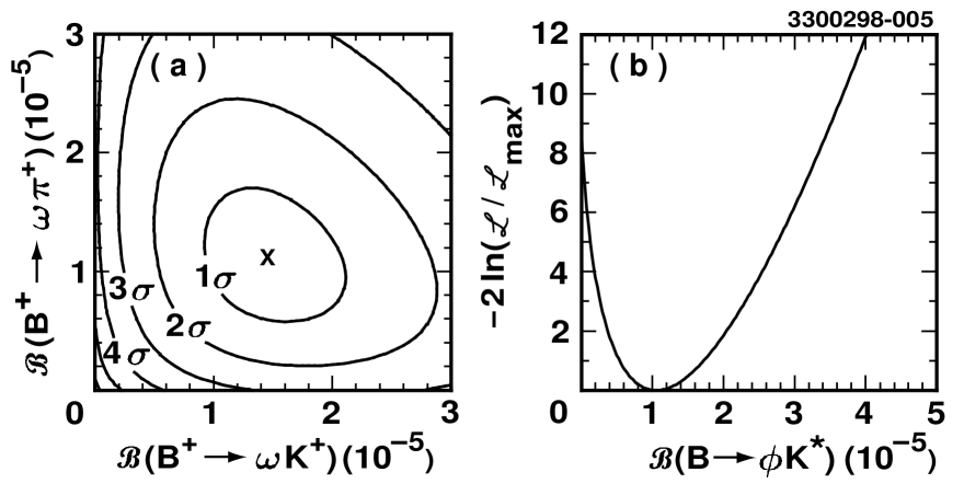
FIG. 2.: (a) Likelihood function contours for $B^{+}\rightarrow\omega h^{+}$; (b) The function $-2\ln{{\cal L}/{\cal L}_{\rm max}}=\chi^{2}-\chi^{2}_{\rm min}$ for $B\rightarrow\phi K^{*}$.

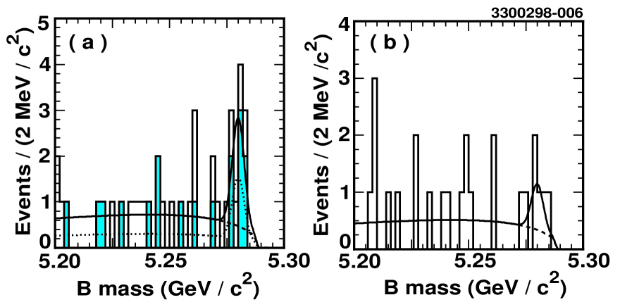
FIG. 3.: Projection onto the variable $M$ for (a) $B^{+}\rightarrow\omega K^{+}$(shaded) and $B^{+}\rightarrow\omega\pi^{+}$(open) and (b) $B\rightarrow\phi K^{*}$. The solid line shows the result of the likelihood fit, scaled to take into account the cuts applied to variables not shown. The dashed line shows the background component, and in (a) the dotted line shows the $B^{+}\rightarrow\omega K^{+}$ fit only.

We also set lower limits on the branching fractions for $B^{+}\rightarrow\omega K^{+}$ and $B^{+}\rightarrow\omega h^{+}$, which could have interesting theoretical implications [17, 18, 19, 20, 21]. We find ${\cal B}(B^{+}\rightarrow\omega K^{+})>8.4\times 10^{-6}$ and ${\cal B}(B^{+}\rightarrow\omega h^{+})>1.6\times 10^{-5}$ at the 90% confidence level. The latter limit would imply that the parameter $\xi$ used in references [19] and [21] is restricted to the region $\xi>0.62$ and $\xi>0.53$, respectively. However, based on reference [19] our measurement of ${\cal B}(B^{+}\rightarrow\phi K^{+})<0.5\times 10^{-5}$ implies that $\xi<0.27$ at the 90% confidence level. Although there is still considerable uncertainty in the theoretical model parameters, these limits illustrate the difficulty in accounting for all our current results with a single phenomenological parameter.

We thank A. Ali, H. Lipkin, J. Rosner, H.-Y. Cheng, and S. Oh for useful discussions. We gratefully acknowledge the effort of the CESR staff in providing us with excellent luminosity and running conditions. This work was supported by the National Science Foundation, the U.S. Department of Energy, Research Corporation, the Natural Sciences and Engineering Research Council of Canada, the A.P. Sloan Foundation, and the Swiss National Science Foundation.

REFERENCES

- [1] M Kobayashi and T. Maskawa, Prog. Theor. Phys. 49, 652 (1973).
- [2] N.G. Deshpande and J. Trampetic, Phys. Rev. D 41, 895 (1990).
- [3] L.-L. Chau et al., Phys. Rev. D 43, 2176 (1991).
- [4] D. Du and Z. Xing, Phys. Lett. B 312, 199 (1993).
- [5] A. Deandrea, N. Di Bartolomeo, R. Gatto, G. Nardulli, Phys. Lett. B 318, 549 (1993); A. Deandrea, N. Di Bartolomeo, R. Gatto, F. Feruglio, G. Nardulli, Phys. Lett. B 320, 170 (1994).
- [6] R. Fleischer, Z. Phys. C 58, 483 (1993).
- [7] A.J. Davies, T. Hayashi, M. Matsuda, and M. Tanimoto, Phys. Rev. D 49, 5882 (1994).
- [8] G. Kramer, W. F. Palmer, and H. Simma, Nucl. Phys. B 428 429 (1994).
- [9] G. Kramer, W. F. Palmer, and H. Simma, Zeit. Phys. C 66 429 (1995).
- [10] D. Du and L. Guo, Z. Phys. C 75, 9 (1997).
- [11] CLEO Collaboration, D.M. Asner et al., Phys. Rev. D 53, 1039 (1996).
- [12] CLEO Collaboration, R. Godang et al., Cornell preprint CLNS 97-1522 (1997, to be published).
- [13] CLEO Collaboration, B.H. Behrens et al., Cornell preprint CLNS 97-1536 (1997, to be published).
- [14] CLEO Collaboration, Y. Kubota et al., Nucl. Instrum. Methods Phys. Res., Sec. A 320, 66 (1992).
- [15] GEANT 3.15, R. Brun et al., CERN DD/EE/84-1.
- [16] Charge conjugate modes are implied throughout this paper.
- [17] H.-Y. Cheng and B. Tseng, preprint hep-ph/9708211, August, 1997.
- [18] M. Ciuchini et al., preprint hep-ph/9708222, November, 1997.
- [19] N.G. Deshpande, B. Dutta, and S. Oh, preprint COLO-HEP-394, December 1997.
- [20] A. S. Dighe, M. Gronau and J. L. Rosner, Phys. Rev. D 57, 1783 (1998).
- [21] A. Ali and C. Greub, Phys. Rev. D 57, 2996 (1998).