Limits on Anomalous $WW\gamma$ and $WWZ$ Couplings

Abstract

Limits on the anomalous $WW\gamma$ and $WWZ$ couplings are presented from a simultaneous fit to the data samples of three gauge boson pair final states in $p\bar{p}$ collisions at $\sqrt{s}=1.8$ TeV: $W\gamma$ production with the $W$ boson decaying to $e\nu$ or $\mu\nu$, $W$ boson pair production with both of the $W$ bosons decaying to $e\nu$ or $\mu\nu$, and $WW$ or $WZ$ production with one $W$ boson decaying to $e\nu$ and the other $W$ boson or the $Z$ boson decaying to two jets. Assuming identical $WW\gamma$ and $WWZ$ couplings, $95\%$ C.L. limits on the anomalous couplings of $-0.30<\Delta\kappa<0.43~{}(\lambda=0)$ and $-0.20<\lambda<0.20~{}(\Delta\kappa=0)$ are obtained using a form factor scale $\Lambda=2.0$ TeV. Limits found under other assumptions on the relationship between the $WW\gamma$ and $WWZ$ couplings are also presented.

Gauge boson self-interactions are a direct consequence of the non-Abelian $SU(2)\times U(1)$ gauge symmetry of the standard model (SM) and are a necessary element to construct unitary and renormalizable theories involving massive gauge bosons [3]. The values of trilinear gauge boson couplings are fully determined in the SM by the gauge structure. The precise determination of the couplings constitutes one of few remaining tests of the SM; any deviation from the SM values would indicate the presence of new physics. Phenomenological bounds on the trilinear gauge boson couplings have been obtained from the precisely measured quantities, such as $(g-2)_{\mu}$, the $b\rightarrow s\gamma$ decay rate, the $Z\rightarrow b{\bar{b}}$ rate and oblique corrections [4]. These bounds are obtained with many assumptions imposed on the couplings. The trilinear gauge boson couplings can be measured directly with fewer assumptions by studying gauge boson pair production processes. Direct measurements of the couplings have been reported by the UA2 [5], CDF [6, 7], DØ [8, 9, 10], and LEP [11] collaborations. Hadron collider experiments have established the electroweak coupling of the $W$ boson to the photon [8] and the existence of the coupling between the $W$ boson and the $Z$ boson [7, 10] by placing constraints on anomalous $WW\gamma$ and $WWZ$ couplings.

The $WW\gamma$ and $WWZ$ vertices are described by a general effective Lagrangian with two overall coupling constants, $g_{WW\gamma}=-e$ and $g_{WWZ}=-e\cdot\cot\theta_{W}$ (where $e$ is the $W^{+}$ charge and $\theta_{W}$ is the weak mixing angle), and six dimensionless coupling parameters, $g_{1}^{V}$, $\kappa_{V}$, and $\lambda_{V}$ ($V=\gamma$ or $Z$), after imposing C, P, and CP invariance [12]. Electromagnetic gauge invariance requires that $g_{1}^{\gamma}=1$, which we assume throughout this paper. The effective Lagrangian becomes that of the SM when $g_{1}^{\gamma}=g_{1}^{Z}=1$ $(\Delta g_{1}^{V}\equiv g_{1}^{V}-1=0)$, $\kappa_{V}=1$ $(\Delta\kappa_{V}\equiv\kappa_{V}-1=0)$, and $\lambda_{V}=0$. Limits on these couplings are usually obtained under the assumption that the $WW\gamma$ and $WWZ$ couplings are equal ($g_{1}^{\gamma}=g_{1}^{Z}=1$, $\Delta\kappa_{\gamma}=\Delta\kappa_{Z}$, and $\lambda_{\gamma}=\lambda_{Z}$).

A different set of parameters, motivated by $SU(2)\times U(1)$ gauge invariance, has been used by the LEP collaborations [13]. This set consists of three independent couplings $\alpha_{B\phi}$, $\alpha_{W\phi}$ and $\alpha_{W}$: $\alpha_{B\phi}\equiv\Delta\kappa_{\gamma}-\Delta g_{1}^{Z}\cos^{2}\theta_{W}$, $\alpha_{W\phi}\equiv\Delta g_{1}^{Z}\cos^{2}\theta_{W}$ and $\alpha_{W}\equiv\lambda_{\gamma}$. The remaining $WWZ$ coupling parameters $\lambda_{Z}$ and $\Delta\kappa_{Z}$ are determined by the relations $\lambda_{Z}=\lambda_{\gamma}$ and $\Delta\kappa_{Z}=-\Delta\kappa_{\gamma}\tan^{2}\theta_{W}+\Delta g_{1}^{Z}$. The HISZ relations [14] which have been used by the DØ and CDF collaborations are also based on this set with the additional constraint $\alpha_{B\phi}=\alpha_{W\phi}$.

Non-SM couplings give rise to a large increase in the cross section of gauge boson pair production processes at high energies. To avoid violation of unitarity, the anomalous couplings are modified by form factors with a scale $\Lambda$ (e.g. $\lambda_{V}(\hat{s})=\lambda_{V}/(1+\hat{s}/\Lambda^{2})^{2}$), which is related to the scale of new physics.

The DØ collaboration has previously reported limits on anomalous $WW\gamma$ and $WWZ$ couplings from the data samples of three gauge boson pair final states: $W\gamma$ production with the $W$ boson decaying to $e\nu$ or $\mu\nu$ [8], $W$ boson pair production with both of the $W$ bosons decaying to $e\nu$ or $\mu\nu$ [9], and $WW$ or $WZ$ production with one $W$ boson decaying to $e\nu$ and the other $W$ boson or the $Z$ boson decaying to two jets [10]. The data samples correspond to an integrated luminosity of approximately 100 pb^-1 collected with the DØ detector during the 1992–93 and 1993–1995 Tevatron collider runs at Fermilab. This report is a culmination of these studies and presents the most stringent limits available on anomalous $WW\gamma$ and $WWZ$ couplings by performing a simultaneous fit to the data samples of the above three final states. Limits are also set on the $\alpha$ parameters, enabling a direct comparison of our results with those of LEP experiments.

The DØ detector and data collection system are described elsewhere [15]. Limits on the anomalous couplings are obtained by a maximum likelihood fit to the transverse energy ($E_{T}$) spectrum of a final state gauge boson or to the $E_{T}$ spectra of the decay leptons from the gauge boson pair. Since the predicted relative increase in the gauge boson pair production cross section with anomalous couplings is greater at higher gauge boson $E_{T}$, fits to the $E_{T}$ spectra provide significantly tighter constraints on anomalous couplings than those from the measurement of the cross section alone. The individual analyses have been described in detail previously [16]. This paper reports only on the simultaneous fit to the three data sets.

In this analysis, as in the previous reports, a binned maximum likelihood fit is performed to the candidate events. The probability $P_{i}$ for observing $N_{i}$ events in a given bin of a kinematical variable is $P_{i}=e^{-(b_{i}+n_{i})}\frac{(b_{i}+n_{i})^{N_{i}}}{N_{i}!}$, where $b_{i}$ is the estimated background, $n_{i}(={\cal L}\epsilon\sigma_{i}(\lambda,\Delta\kappa))$ is the expected signal, ${\cal L}$ is the integrated luminosity, $\epsilon$ is the detection efficiency, and $\sigma_{i}$ is the theoretical cross section which is a function of anomalous couplings, $\lambda$ and $\Delta\kappa$. The joint probability $P$ for all the kinematical bins that are fitted is $P=\prod^{N_{bin}}_{i=1}P_{i}$. Since the variables $b_{i},{\cal L}$, $\epsilon$ and the normalization of the predicted theoretical cross section are estimated quantities with some uncertainty and do not depend on $\lambda$ and $\Delta\kappa$, we assign Gaussian prior distributions and integrate over the possible ranges; $P^{\prime}\propto\int{\cal G}_{f_{n}}df_{n}\int{\cal G}_{f_{b}}df_{b}\prod^{N_{bin}}_{i=1}\frac{e^{-(f_{n}n_{i}+f_{b}b_{i})}(f_{n}n_{i}+f_{b}b_{i})^{N_{i}}}{N_{i}!}$, where ${\cal G}_{f_{b}}$ and ${\cal G}_{f_{n}}$ are Gaussian functions with standard deviation $\sigma_{b}$ and $\sigma_{n}$ for the background and the signal, respectively. For convenience, the log-likelihood, $L=-\log P^{\prime}$, is used. When the simultaneous fit is performed on the three data sets, correlations between $\sigma_{b}$ and $\sigma_{n}$ for different final states are carefully taken into account.

In Table I, the $95\%$ C.L. limits on anomalous $WW\gamma$ couplings from the $W\gamma$ analysis are listed. The $W\gamma$ candidate events are selected by requiring an isolated high $E_{T}$ electron or muon, large missing transverse energy ($\hbox to0.0pt{\kern 2.5pt/\hss}E_{T}$) and an isolated high $E_{T}$ photon. The limits are obtained from a binned maximum likelihood fit to the $E_{T}$ spectrum of the photons. In this process, only $\lambda_{\gamma}$ and $\Delta\kappa_{\gamma}$ couplings are involved.

In Table II, the $95\%$ C.L. limits from the $WW\rightarrow$ dilepton analysis are listed. The $WW\rightarrow$ dilepton candidate events are selected by requiring two high $E_{T}$ leptons ($ee$, $e\mu$, or $\mu\mu$) and large $\hbox to0.0pt{\kern 2.5pt/\hss}E_{T}$. The limits are obtained from a maximum likelihood fit to the number of observed candidate events in two-dimensional $E_{T}$ bins of the decay leptons from the $W$ boson pair.

In Table III, the $95\%$ C.L. limits from the $WW/WZ\rightarrow e\nu jj$ analysis are listed. The $WW/WZ\rightarrow e\nu jj$ candidate events are selected by requiring an isolated high $E_{T}$ electron, large $\hbox to0.0pt{\kern 2.5pt/\hss}E_{T}$, and two high $E_{T}$ jets. The invariant mass of the two jet system must be consistent with that of the $W$ or $Z$ boson. Limits are obtained from a binned maximum likelihood fit to the $E_{T}$ spectrum of the $W$ boson calculated from the electron $E_{T}$ and $\hbox to0.0pt{\kern 2.5pt/\hss}E_{T}$, using four sets of relationships between the $WW\gamma$ and $WWZ$ couplings: (i) $\Delta\kappa\equiv\Delta\kappa_{\gamma}=\Delta\kappa_{Z},\lambda\equiv\lambda_{\gamma}=\lambda_{Z}$, (ii) HISZ relations, (iii) varying the $WWZ$ couplings while the $WW\gamma$ couplings are fixed to the SM values, and (iv) varying the $WW\gamma$ couplings while the $WWZ$ couplings are fixed to the SM values. Two values of $\Lambda$, 1.5 and 2.0 TeV, are used.

Tables I–III are reproduced from the previous reports. Figure 1 contains the $95\%$ C.L. one-degree of freedom exclusion contours [17] from the $W\gamma$, $WW\rightarrow$ dilepton, and $WW/WZ\rightarrow e\nu jj$ analyses. The contours that represent the unitarity constraint [18] for individual processes are omitted in Fig. 1.

In Table IV, the $95\%$ C.L. limits from a simultaneous fit to the three data sets are presented. The common uncertainties, those on the integrated luminosity ($5.3\%$) and the theoretical cross section of the gauge boson pair production ($7\%$), are factored out and included only once in the integration. Correlations in the uncertainties on the electron and muon selection efficiencies between the data sets of the 1992–1993 and 1993–1995 runs are properly taken into account for individual final states. Correlations in the uncertainties on the electron and muon selection efficiencies between different final states are ignored, since the uncertainties themselves are small and have practically no effect on the limits. Correlations in the uncertainties on the background estimates between the data sets of the 1992–1993 and 1993–1995 runs are properly taken into account for individual final states. The uncertainties on the background estimates between different final states are assumed to be uncorrelated, since the dominant sources of uncertainties are different for the three final states. Figure 2(a) shows the contour limits when the $WW\gamma$ and $WWZ$ couplings are assumed to be equal. Figure 2(b) shows the contour limits assuming HISZ relations. In Fig. 2(c), the contour limits on anomalous $WWZ$ couplings are shown assuming the SM $WW\gamma$ couplings. The $U(1)$ point ($\kappa_{Z}=0$, $\lambda_{Z}=0$ and $g_{1}^{Z}=0$) indicated in the figure, which implies that there is no coupling between the $W$ boson and the $Z$ boson, is excluded at the 99.99% C.L. In Fig. 2(d), the contour limits on anomalous $WW\gamma$ couplings are shown assuming the SM $WWZ$ couplings. The $U(1)$ point ($\kappa_{\gamma}=0$, and $\lambda_{\gamma}=0$) indicated in the figure, which implies that the $W$ boson couples to the photon with the electromagnetic interactions only, is excluded at the 99.7% C.L. The innermost and middle curves are $95\%$ C.L. one- and two-degree of freedom exclusion contours, respectively [17]. The outermost curve is the constraint from the unitarity condition with $\Lambda=1.5$ TeV.

In Table V, the $95\%$ C.L. limits on the $\alpha$ parameters from a simultaneous fit to the three data sets are presented. Limits on $\Delta g_{1}^{Z}$ are obtained, from the limits on $\alpha_{W\phi}$ for $\alpha_{B\phi}=\alpha_{W}=0$. For comparison, limits from the OPAL collaboration [11] are also listed in Table V. Limits from other LEP collaborations are similar to those from OPAL. Figure 3(a) shows the contour limits in the $\alpha_{W}$-$\alpha_{B\phi}$ plane, when $\alpha_{W\phi}=0$. Figure 3(b) shows the contour limits in the $\alpha_{W}$-$\alpha_{W\phi}$ plane, when $\alpha_{B\phi}=0$.

In summary, limits on the anomalous $WW\gamma$ and $WWZ$ couplings are obtained from a simultaneous fit to the data samples of three gauge boson pair final states. These limits are the tightest limits available on the anomalous $WW\gamma$ and $WWZ$ couplings.

We thank the staffs at Fermilab and collaborating institutions for their contributions to this work, and acknowledge support from the Department of Energy and National Science Foundation (U.S.A.), Commissariat à L’Energie Atomique (France), State Committee for Science and Technology and Ministry for Atomic Energy (Russia), CAPES and CNPq (Brazil), Departments of Atomic Energy and Science and Education (India), Colciencias (Colombia), CONACyT (Mexico), Ministry of Education and KOSEF (Korea), and CONICET and UBACyT (Argentina).

FIG. 1.: Contour limits on anomalous couplings for $\Lambda=1.5$ TeV. For the $WW\rightarrow$ dilepton and $WW/WZ\rightarrow e\nu jj$ contour limits, the $WW\gamma$ and $WWZ$ couplings are assumed to be equal. The contours plotted in Figs. 1–3 are accurate to $\pm 0.02$ due to MC statistics.

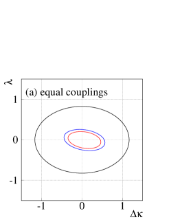
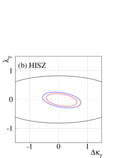
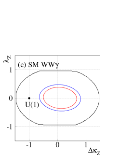
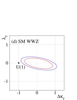
FIG. 2.: Contour limits on anomalous couplings from a simultaneous fit to the data sets of $W\gamma$, $WW\rightarrow$ dilepton, and $WW/WZ\rightarrow e\nu jj$ final states for $\Lambda=1.5$ TeV: (a) $\Delta\kappa\equiv\Delta\kappa_{\gamma}=\Delta\kappa_{Z},\lambda\equiv\lambda_{\gamma}=\lambda_{Z}$; (b) HISZ relations; (c) SM $WW\gamma$ couplings; and (d) SM $WWZ$ couplings. (a), (c), and (d) assume that $\Delta g_{1}^{Z}=0$. The innermost and middle curves are $95\%$ C.L. one- and two-degree of freedom exclusion contours, respectively. The outermost curve is the constraint from the unitarity condition. In (d), the unitarity contour is located outside of the boundary of the plot.

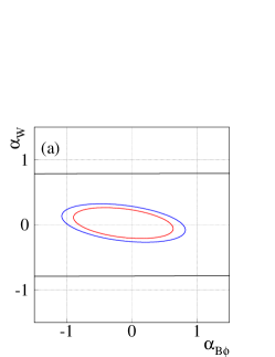
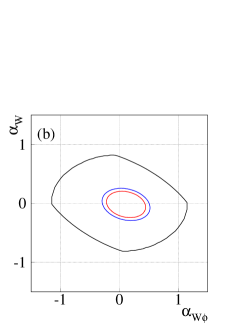
FIG. 3.: Contour limits on anomalous couplings from a simultaneous fit to the data sets of the $W\gamma$, $WW\rightarrow$ dilepton, and $WW/WZ\rightarrow e\nu jj$ final states for $\Lambda=1.5$ TeV: (a) $\alpha_{W}$ vs $\alpha_{B\phi}$ when $\alpha_{W\phi}=0$; and (b) $\alpha_{W}$ vs $\alpha_{W\phi}$ when $\alpha_{B\phi}=0$. The innermost and middle curves are $95\%$ C.L. one- and two-degree of freedom exclusion contours, respectively. The outermost curve is the constraint from the unitarity condition.

TABLE I.: Limits at 95% C.L. from the $W\gamma$ analysis.

	$\Lambda=1.5$ TeV
$\lambda_{\gamma}$ ($\Delta\kappa_{\gamma}=0$)	$-0.31,~{}0.29$
$\Delta\kappa_{\gamma}$ ($\lambda_{\gamma}=0$)	$-0.93,~{}0.94$

TABLE II.: Limits at 95% C.L. from the $WW\rightarrow$ dilepton analysis.

	$\Lambda=1.5$ TeV
$\lambda_{\gamma}=\lambda_{Z}$ ($\Delta\kappa_{\gamma}=\Delta\kappa_{Z}=0$)	$-0.53,~{}0.56$
$\Delta\kappa_{\gamma}=\Delta\kappa_{Z}$ ($\lambda_{\gamma}=\lambda_{Z}=0$)	$-0.62,~{}0.77$
$\lambda_{\gamma}$(HISZ) ($\Delta\kappa_{\gamma}=0$)	$-0.53,~{}0.56$
$\Delta\kappa_{\gamma}$(HISZ) ($\lambda_{\gamma}=0$)	$-0.92,~{}1.20$

TABLE III.: Limits at 95% C.L. from the $WW/WZ\rightarrow e\nu jj$ analysis.

$\Lambda$	$1.5$ TeV	$2.0$ TeV
$\lambda_{\gamma}=\lambda_{Z}$ ($\Delta\kappa_{\gamma}=\Delta\kappa_{Z}=0$)	$-0.36,~{}0.39$	$-0.34,~{}0.36$
$\Delta\kappa_{\gamma}=\Delta\kappa_{Z}$ ($\lambda_{\gamma}=\lambda_{Z}=0$)	$-0.47,~{}0.63$	$-0.43,~{}0.59$
$\lambda_{\gamma}$(HISZ) ($\Delta\kappa_{\gamma}=0$)	$-0.36,~{}0.39$	$-0.34,~{}0.36$
$\Delta\kappa_{\gamma}$(HISZ) ($\lambda_{\gamma}=0$)	$-0.56,~{}0.85$	$-0.53,~{}0.78$
$\lambda_{Z}$(SM $WW\gamma$) ($\Delta\kappa_{Z}=\Delta g^{Z}_{1}=0$)	$-0.40,~{}0.43$	$-0.37,~{}0.40$
$\Delta\kappa_{Z}$(SM $WW\gamma$) ($\lambda_{Z}=\Delta g^{Z}_{1}=0$)	$-0.60,~{}0.79$	$-0.54,~{}0.72$
$\Delta g^{Z}_{1}$(SM $WW\gamma$) ($\lambda_{Z}=\Delta\kappa_{Z}=0$)	$-0.64,~{}0.89$	$-0.60,~{}0.81$
$\lambda_{\gamma}$(SM $WWZ$) ($\Delta\kappa_{\gamma}=0$)	$-1.21,~{}1.25$	–
$\Delta\kappa_{\gamma}$(SM $WWZ$) ($\lambda_{\gamma}=0$)	$-1.38,~{}1.70$	–

TABLE IV.: Limits at 95% C.L. from a simultaneous fit to the $W\gamma$, $WW\rightarrow$ dilepton and $WW/WZ\rightarrow e\nu jj$ data samples. The four sets of limits apply the same assumptions as the four components (a), (b), (c) and (d), respectively, of Fig. 2.

$\Lambda$	$1.5$ TeV	$2.0$ TeV
$\lambda_{\gamma}=\lambda_{Z}$ ($\Delta\kappa_{\gamma}=\Delta\kappa_{Z}=0$)	$-0.21,~{}0.21$	$-0.20,~{}0.20$
$\Delta\kappa_{\gamma}=\Delta\kappa_{Z}$ ($\lambda_{\gamma}=\lambda_{Z}=0$)	$-0.33,~{}0.46$	$-0.30,~{}0.43$
$\lambda_{\gamma}$(HISZ) ($\Delta\kappa_{\gamma}=0$)	$-0.21,~{}0.21$	$-0.20,~{}0.20$
$\Delta\kappa_{\gamma}$(HISZ) ($\lambda_{\gamma}=0$)	$-0.39,~{}0.61$	$-0.37,~{}0.56$
$\lambda_{Z}$(SM $WW\gamma$) ($\Delta\kappa_{Z}=\Delta g^{Z}_{1}=0$)	$-0.33,~{}0.37$	$-0.31,~{}0.34$
$\Delta\kappa_{Z}$(SM $WW\gamma$) ($\lambda_{Z}=\Delta g^{Z}_{1}=0$)	$-0.46,~{}0.64$	$-0.42,~{}0.59$
$\Delta g^{Z}_{1}$(SM $WW\gamma$) ($\lambda_{Z}=\Delta\kappa_{Z}=0$)	$-0.56,~{}0.86$	$-0.52,~{}0.78$
$\lambda_{\gamma}$(SM $WWZ$) ($\Delta\kappa_{\gamma}=0$)	$-0.27,~{}0.25$	$-0.26,~{}0.24$
$\Delta\kappa_{\gamma}$(SM $WWZ$) ($\lambda_{\gamma}=0$)	$-0.63,~{}0.75$	$-0.59,~{}0.72$

TABLE V.: Limits at 95% C.L. on $\alpha$ parameters from a simultaneous fit to the $W\gamma$, $WW\rightarrow$ dilepton and $WW/WZ\rightarrow e\nu jj$ data samples. Limits from the OPAL collaboration are also listed for comparison.

$\Lambda$	$1.5$ TeV	$2.0$ TeV	OPAL
$\alpha_{B\phi}$ ($\alpha_{W\phi}=\alpha_{W}=0$)	$-0.81,~{}0.61$	$-0.77,~{}0.58$	$-1.6,~{}2.7$
$\alpha_{W\phi}$ ($\alpha_{B\phi}=\alpha_{W}=0$)	$-0.24,~{}0.46$	$-0.22,~{}0.44$	$-0.55,~{}0.64$
$\alpha_{W}$ ($\alpha_{B\phi}=\alpha_{W\phi}=0$)	$-0.21,~{}0.21$	$-0.20,~{}0.20$	$-0.78,~{}1.19$
$\Delta g^{Z}_{1}$ ($\alpha_{B\phi}=\alpha_{W}=0$)	$-0.31,~{}0.60$	$-0.29,~{}0.57$	$-0.75,~{}0.77$

REFERENCES

- [1] Visitor from Universidad San Francisco de Quito, Quito, Ecuador.
- [2] Visitor from IHEP, Beijing, China.
- [3] C. H. Llewellyn Smith, Phys. Lett. B 46, 233 (1973); J. M. Cornwall, D. N. Levin and G. Tiktopoulos, Phys. Rev. Lett. 30, 1268 (1973); Phys. Rev. D 10, 1145 (1973); S. D. Joglekar, Ann. Phys. 83, 427 (1974).
- [4] H. Aihara et al., in Electroweak Symmetry Breaking and New Physics at the TeV Scale edited by T. L. Barklow et al., World Scientific 1996, p.488; F. M. Renard, S. Spagnolo and C. Verzegnassi, Phys. Lett. B 409, 398 (1997);J. J. van der Bij and B. Kastening, Phys. Rev. D 57, 2903 (1998)
- [5] UA2 Collaboration, J. Alitti et al., Phys. Lett. B277, 194 (1992).
- [6] CDF Collaboration, F. Abe et al., Phys. Rev. Lett. 74, 1936 (1995); ibid. 78, 4536 (1997).
- [7] CDF Collaboration, F. Abe et al., Phys. Rev. Lett. 75, 1017 (1995);
- [8] DØ Collaboration, S. Abachi et al., Phys. Rev. Lett. 75, 1034 (1995); ibid. 78, 3634 (1997).
- [9] DØ Collaboration, S. Abachi et al., Phys. Rev. Lett. 75, 1023 (1995); DØ Collaboration, B. Abbott et al., hep-ex/9803004 and FERMILAB-Pub-98/076-E, submitted to Phys. Rev. D.
- [10] DØ Collaboration, S. Abachi et al., Phys. Rev. Lett. 77, 3303 (1996); DØ Collaboration, B. Abbott et al., ibid. 79, 1441 (1997).
- [11] OPAL Collaboration, K. Ackerstaff et al., Phys. Lett. B 397, 147 (1997); OPAL Collaboration, K. Ackerstaff et al., hep-ex/9709023 and CERN-PPE/97-125, submitted to Z. Phys. C, September 1997; DELPHI Collaboration, P. Abreu et al., Phys. Lett. B 397, 158 (1997); L3 Collaboration, M. Acciarri et al., ibid. 398, 223 (1997); ibid. 403, 168 (1997); ibid. 413, 176 (1997); ALEPH Collaboration, R. Barate et al., CERN-PPE/97-166, submitted to Phys. Lett. B, December 1997.
- [12] K. Hagiwara, R. D. Peccei, D. Zeppenfeld and K. Hikasa, Nucl. Phys. B282, 253 (1987). We use in our Monte Carlo program.
- [13] G. Gounaris et al., in Physics at LEP2 edited by G. Altarelli, T. Sjöstrand and F. Zwirner, CERN 96-01, 1996 (unpublished), p. 525.
- [14] K. Hagiwara, S. Ishihara, R. Szalapski, and D. Zeppenfeld, Phys. Rev. D 48, 2182 (1993); Phys. Lett. B 283, 353 (1992). The couplings are related to the couplings as follows: , and .
- [15] DØ Collaboration, S. Abachi et al., Nucl. Instrum. Methods in Phys. Res. A338, 185 (1994).
- [16] DØ Collaboration, S. Abachi et al., Phys. Rev. D 56, 6742 (1997); H. Johari, Ph.D. thesis, Northeastern University, 1995 (unpublished); M. L. Kelly, Ph.D. thesis, University of Notre Dame, 1996 (unpublished); T. Fahland, Ph.D. thesis, Brown University, 1996 (unpublished); A. Sánchez-Hernández, Ph.D. thesis, CINVESTAV, Mexico City, Mexico, 1997 (unpublished); P. Bloom, Ph.D. thesis, University of California, Davis, 1998 (unpublished). These theses are available from http://www-d0.fnal.gov/publications_talks/ thesis/thesis.html.
- [17] One- and two-degree of freedom exclusion contours are obtained by cutting the log likelihood surface at 1.92 and 3.0 below the maximum. These values correspond to the 95% confidence levels for the cases when only one free parameter is allowed (1.92) and two free parameters are allowed (3.00) in the fit.
- [18] U. Baur and D. Zeppenfeld, Phys. Lett. B 201, 383 (1988). U. Baur provided the programs to calculate the unitarity contours.