First Observation of the Cabibbo Suppressed Decay $B^{+}\rightarrow\bar{D}^{0}K^{+}$

Abstract

We have observed the decay $B^{+}\rightarrow\bar{D}^{0}K^{+}$, using 3.3 million $B\bar{B}$ pairs collected with the CLEO II detector at the Cornell Electron Storage Ring. We find the ratio of branching fractions $R\equiv{\cal B}(B^{+}\rightarrow\bar{D}^{0}K^{+})/{\cal B}(B^{+}\rightarrow\bar{D}^{0}\pi^{+})=0.055\pm 0.014\pm 0.005$.

Several authors [1] have devised methods for measuring the phase $\gamma\approx\arg(V^{*}_{ub})$ of the Cabibbo-Kobayashi-Maskawa (CKM) [2] unitarity triangle, using decays of the type $B\rightarrow DK$. Comparison between these measurements and results from other $B$ and $K$ decays may be used to test the CKM model of $CP$ violation. $CP$ violation could be manifested in $B\rightarrow DK$ in the interference between a $\bar{b}\rightarrow\bar{c}$ and a $\bar{b}\rightarrow\bar{u}$ amplitude (Figure 1), detected when the $D$ meson is observed in a final state accessible to both $D^{0}$ and $\bar{D}^{0}$.

The data used in this analysis were produced in $e^{+}e^{-}$ annihilations at the Cornell Electron Storage Ring (CESR), and collected with the CLEO II detector [3]. The data consist of $3.1~{}{\rm fb}^{-1}$ taken at the $\Upsilon$(4S) resonance, containing approximately 3.3 million $B\bar{B}$ pairs. To study the continuum $e^{+}e^{-}\rightarrow q\bar{q}$ background, we use $1.6~{}{\rm fb}^{-1}$ of off-resonance data, taken 60 MeV below the $\Upsilon$(4S) peak.

CLEO II is a general-purpose solenoidal magnet detector. The momenta of charged particles are measured in a tracking system, consisting of a 6-layer straw tube chamber, a 10-layer precision drift chamber, and a 51-layer main drift chamber, all operating inside a 1.5 T superconducting solenoid. The main drift chamber also provides measurements of the specific ionization, $dE/dx$, which we use for particle identification. Photons are detected in a 7800-CsI crystal electromagnetic calorimeter inside the magnet coil. Muons are identified using proportional counters placed at various depths in the magnet return iron.

We reconstruct $\bar{D}^{0}$ candidates in the decay modes $K^{+}\pi^{-}$, $K^{+}\pi^{-}\pi^{0}$, or $K^{+}\pi^{-}\pi^{+}\pi^{-}$ (reference to the charge-conjugate state is implied). Pion and kaon candidate tracks are required to originate from the interaction point and satisfy criteria designed to reject spurious tracks. Muons are rejected by requiring that the tracks stop in the first five interaction lengths of the muon chambers. Electrons are rejected using $dE/dx$ and the ratio of the track momentum to the associated calorimeter shower energy. The $\bar{D}^{0}$ daughter tracks are required to have $dE/dx$ consistent with their particle hypothesis to within three standard deviations ($\sigma$). Neutral pion candidates are reconstructed from pairs of isolated calorimeter showers with invariant mass within 15 MeV (approximately $2.5\sigma$) of the nominal $\pi^{0}$ mass. The lateral shapes of the showers are required to be consistent with those of photons. We require a minimum energy of 30 MeV for showers in the barrel part of the calorimeter, and 50 MeV for endcap showers. At least one of the two $\pi^{0}$ showers is required to be in the barrel. The $\pi^{0}$ candidates are kinematically fitted with the invariant mass constrained to be the $\pi^{0}$ mass.

The invariant mass of the $\bar{D}^{0}$ candidate, $M(D)$, is required to be within 60 MeV of the nominal $\bar{D}^{0}$ mass. The $M(D)$ resolution, $\sigma_{M(D)}$, is 9 MeV in the $K^{+}\pi^{-}$ mode, 13 MeV in the $K^{+}\pi^{-}\pi^{0}$ mode, and 7 MeV in the $K^{+}\pi^{-}\pi^{+}\pi^{-}$ mode. The loose $M(D)$ requirement leaves a broad sideband to assess the background.

$B^{+}$ candidates are formed by combining a $\bar{D}^{0}$ candidate with a “hard” kaon candidate track. For each $B^{+}$ candidate, we calculate the beam-constrained mass, $M_{bc}\equiv\sqrt{E_{\rm b}^{2}-p_{B}^{2}}$, where $p_{B}$ is the $B^{+}$ candidate momentum and $E_{\rm b}$ is the beam energy. $M_{bc}$ peaks at the nominal $B^{+}$ mass for signal, with a resolution of $\sigma_{M_{bc}}=2.6$ MeV, determined mostly by the beam energy spread. We accept candidates with $M_{bc}>5.230$ GeV. We define the energy difference, $\Delta E\equiv E_{D}+\sqrt{p_{K}^{2}+M_{K}^{2}}-E_{\rm b}$, where $E_{D}$ is the measured energy of the $\bar{D}^{0}$ candidate, $p_{K}$ is the momentum of the hard kaon candidate, and $M_{K}$ is the nominal kaon mass. Signal events peak around $\Delta E=0$, with a resolution of 24 MeV in the $K^{+}\pi^{-}$ mode, 27 MeV in the $K^{+}\pi^{-}\pi^{0}$ mode, and 20 MeV in the $K^{+}\pi^{-}\pi^{+}\pi^{-}$ mode. We require $-100<\Delta E<200$ MeV.

The largest source of background is the Cabibbo allowed decay $B^{+}\rightarrow\bar{D}^{0}\pi^{+}$, distributed around $\Delta E=48$ MeV. Taking into account correlations between $\Delta E$ and $M(D)$, the $\Delta E$ separation between signal and $B^{+}\rightarrow\bar{D}^{0}\pi^{+}$ is about $2.3\sigma$ in all three modes. The only additional variable which provides significant $K-\pi$ separation is $dE/dx$ of the hard kaon candidate. The $dE/dx$ separation between kaons and pions in the relevant momentum range of $2.1-2.5$ GeV is approximately $1.5\sigma$. Our $dE/dx$ variable is chosen such that pions are distributed approximately as a zero-centered, unit-r.m.s. Gaussian, and kaons are centered around $-1.4$, with a width of about 0.9.

Other sources of $B\bar{B}$ background are $B\rightarrow\bar{D}^{*}\pi^{+}$, $B^{+}\rightarrow\bar{D}^{0}\rho^{+}$, and events with a misreconstructed $\bar{D}^{0}$ which pass the selection criteria. Such $B\bar{B}$ events tend to have low $\Delta E$ and broad $M_{bc}$ distributions. Continuum $e^{+}e^{-}\rightarrow q\bar{q}$ events also contribute to the background. We reject 69% of the continuum and retain 87% of the signal by requiring $|\cos\theta_{s}|<0.9$, where $\theta_{s}$ is the angle between the sphericity axis of the $B^{+}$ candidate and that of the rest of the event. The sphericity axis, ${\boldmath\bf s}$, of a set of momentum vectors, $\{{\boldmath\bf p}_{i}\}$, is the axis for which $\sum_{i}|{\boldmath\bf p}_{i}\times{\boldmath\bf s}|^{2}$ is minimized.

In addition to the above variables, discrimination between signal and continuum background is obtained from $\cos\theta_{B}$, where $\theta_{B}$ is the angle between the $B^{+}$ candidate momentum and the beam axis, and by using a Fisher discriminant [4]. The Fisher discriminant is a linear combination, ${\cal F}\equiv\sum_{i=1}^{11}\alpha_{i}y_{i}$, where the coefficients $\alpha_{i}$ are chosen so as to maximize the separation between $B\bar{B}$ and continuum Monte Carlo samples. The eleven variables, $y_{i}$, are $|\cos\theta_{thr}|$ (the cosine of the angle between the $B^{+}$ candidate thrust axis and the beam axis), the ratio of the Fox-Wolfram moments $H_{2}/H_{0}$ [5], and nine variables measuring the scalar sum of the momenta of tracks and showers from the rest of the event in nine, $10^{\circ}$ angular bins centered about the candidate’s thrust axis. Signal events peak around ${\cal F}=0.4$, while continuum events peak at ${\cal F}=2$, both with approximately unit r.m.s.

18.8% of the events have more than one $B^{+}$ candidate, reconstructed in any of the three modes, which satisfies the selection criteria. In such events we select the best candidate, defined to have the smallest $\chi^{2}\equiv[(M_{bc}-M_{B})/\sigma_{M_{bc}}]^{2}+[(M(D)-M_{D})/\sigma_{M(D)}]^{2}$, where $M_{B}$ and $M_{D}$ are the nominal $B$ and $D$ masses, respectively. We verify that the distribution of the number of candidates per event in the Monte Carlo agrees well with the data.

The efficiency of signal events to pass all the requirements is $0.4412\pm 0.0029$ for the $K^{+}\pi^{-}$ mode, $0.1688\pm 0.0016$ for the $K^{+}\pi^{-}\pi^{0}$ mode, and $0.2186\pm 0.0024$ for the $K^{+}\pi^{-}\pi^{+}\pi^{-}$ mode. The efficiencies are determined using a detailed GEANT-based Monte Carlo simulation [8], and the errors quoted are due to Monte Carlo statistics.

The number of data events that satisfy the selection criteria, $N_{e}$, is 1221 in the $K^{+}\pi^{-}$ mode, 5249 in the $K^{+}\pi^{-}\pi^{0}$ mode , and 7353 in the $K^{+}\pi^{-}\pi^{+}\pi^{-}$ mode. The fraction of signal events in the data samples is found mode-by-mode using an unbinned maximum likelihood fit. We define the likelihood function

$${\cal L}=\prod_{e=1}^{N_{e}}\left[\sum_{t=1}^{7}{\cal P}_{t}(e)f_{t}\right],$$ (1)

where ${\cal P}_{t}(e)$ is the normalized probability density function (PDF) for events of type $t$, evaluated on event $e$, and $f_{t}$ is the fraction of such events in the data sample. The seven event types in the sum are 1) signal, 2) $B^{+}\rightarrow\bar{D}^{0}\pi^{+}$, 3) $B\rightarrow\bar{D}^{*}\pi^{+}+\bar{D}^{0}\rho^{+}$, 4) a hard kaon or 5) pion in combinatoric $B\bar{B}$ events with a misreconstructed $\bar{D}^{0}$, and 6) a hard kaon or 7) pion in continuum events. The fit maximizes ${\cal L}$ by varying the seven fractions, $f_{t}$, subject to the constraint $\sum_{t}f_{t}=1$.

The PDF’s are analytic, six-dimensional functions of the variables $\Delta E$, $dE/dx$ of the hard kaon candidate, $M(D)$, $M_{bc}$, ${\cal F}$, and $\cos\theta_{B}$. The PDF’s are mostly products of six one-dimensional functions, except for correlations between $\Delta E$, $M(D)$, and $M_{bc}$ in the $B^{+}\rightarrow\bar{D}^{0}K^{+}$ and $B^{+}\rightarrow\bar{D}^{0}\pi^{+}$ PDF’s.

The $dE/dx$ distributions of $K^{\pm},\pi^{\pm}$ are parameterized using a Gaussian distribution, whose parameters depend linearly on the track momentum. The parameterization is determined by studying pure samples of kaons and pions in data, tagged in the decay chain $D^{*+}\rightarrow D^{0}\pi^{+}$, $D^{0}\rightarrow K^{-}\pi^{+}$. The parameterization in the other variables is obtained from the off-resonance data for the continuum PDF’s and from Monte Carlo for the $B\bar{B}$ PDF’s.

The distribution of $B^{+}\rightarrow\bar{D}^{0}K^{+}$ and $B^{+}\rightarrow\bar{D}^{0}\pi^{+}$ events in $\Delta E-M(D)-M_{bc}$ space is parameterized using the sum of two three-dimensional Gaussians, which are rotated to account for correlations. For $B\rightarrow\bar{D}^{*}\pi^{+}+\bar{D}^{0}\rho^{+}$ events we use the sum of two Gaussians to parameterize the $M_{bc}$ and $\Delta E$ distributions, and a Gaussian plus a bifurcated Gaussian for the $M(D)$ distribution. These distributions are essentially uncorrelated due to the requirement $\Delta E>-100$ MeV. For $B\bar{B}$ events with a misreconstructed $\bar{D}^{0}$ we use a third-order polynomial to parameterize the $\Delta E$ distribution, and a first-order polynomial plus a Gaussian for the $M(D)$ distribution. The Gaussian is about three times broader than the $M(D)$ resolution, and models the peaking which arises due to the selection of the best candidate in the event. The $M_{bc}$ distribution is parameterized using the Argus function [6] $f(M_{bc})\propto M_{bc}\sqrt{1-(M_{bc}/E_{b})^{2}}\exp[-a(1-(M_{bc}/E_{b})^{2})]$, plus a Gaussian, which reflects mostly $B\rightarrow\bar{D}^{(*)}\pi^{+}$ or $B^{+}\rightarrow\bar{D}^{0}\rho^{+}$ events in which we misreconstruct a $\bar{D}^{0}$.

We use a first-order polynomial to parameterize the $\Delta E$ distribution of continuum events, and a first-order polynomial plus a Gaussian for their $M(D)$ distribution. The Gaussian peaking is due both to real $\bar{D}^{0}$’s and to the selection of the best candidate in the event. The $M_{bc}$ distribution is parameterized using an Argus function whose sharp edge is smeared by adding a bifurcated Gaussian to account for the beam energy spread. We use the function $1-\xi\cos^{2}\theta_{B}$ to parameterize the $\cos\theta_{B}$ distributions, and bifurcated Gaussians for the $\cal F$ distributions.

The results of the maximum likelihood fits are summarized in Table I. Averaging over the three modes, we find $R\equiv{\cal B}(B^{+}\rightarrow\bar{D}^{0}K^{+})/{\cal B}(B^{+}\rightarrow\bar{D}^{0}\pi^{+})=0.055\pm 0.014$ (statistical). This is consistent with the value $(f_{K}/f_{\pi})^{2}\tan^{2}\theta_{c}\approx 0.07$, expected from factorization, with $a_{2}\ll a_{1}$ [7]. The $\chi^{2}$ of the average is $1.2$ for two degrees of freedom, indicating the consistency among the results obtained with the three decay modes. To illustrate the significance of the signal yield, contour plots of $-2\ln{\cal L}$ vs. the number of $B^{+}\rightarrow\bar{D}^{0}K^{+}$ and $B^{+}\rightarrow\bar{D}^{0}\pi^{+}$ events are shown in Figure 2. The curves represent $n\sigma$ contours, corresponding to the increase in $-2\ln{\cal L}$ by $n^{2}$ over the minimum value.

TABLE I.: Results of the maximum likelihood fits. $N_{DK}$ and $N_{D\pi}$ are the numbers of $B^{+}\rightarrow\bar{D}^{0}K^{+}$ and $B^{+}\rightarrow\bar{D}^{0}\pi^{+}$ events found in the fit, respectively. Errors are statistical only. The statistical significance of the signal yield is determined from $-2\ln{\cal L}$ by fixing the number of signal events at zero and refitting the data.

Mode:	$K^{+}\pi^{-}$	$K^{+}\pi^{-}\pi^{0}$	$K^{+}\pi^{-}\pi^{+}\pi^{-}$
$N_{DK}$	$16.5\pm 5.9$	$13.5\pm 8.7$	$21.5\pm 7.8$
$N_{D\pi}$	$240\pm 15$	$379\pm 22$	$326\pm 20$
$N_{DK}$ significance	$4.2\sigma$	$1.8\sigma$	$3.8\sigma$
$N_{DK}/N_{D\pi}$	$0.069\pm 0.026$	$0.035\pm 0.023$	$0.066\pm 0.025$

The quality of the fit is illustrated in Figure 3a, showing projections of the data onto $dE/dx$ and $\Delta E$ for events in the $B^{+}\rightarrow\bar{D}^{0}K^{+}$ region, defined by ${\cal F}<1.6$, $|M_{bc}-5280\ {\rm MeV}|<5\ {\rm MeV}$, $|M(D)-1864.5\ {\rm MeV}|<20\ {\rm MeV}$, $-50<\Delta E<10\ {\rm MeV}$, $dE/dx<-0.75$. Requiring that events fall within this $B^{+}\rightarrow\bar{D}^{0}K^{+}$ region reduces the signal efficiency by about 50%, but strongly suppresses the background. Overlaid on the data are projections of the fit function. The fit function is the sum of the PDF’s, each weighted by the number of corresponding events found in the fit and multiplied by the efficiency of the corresponding event type to be in the $B^{+}\rightarrow\bar{D}^{0}K^{+}$ region. In Figure 3b we show projection plots for events in the $B^{+}\rightarrow\bar{D}^{0}\pi^{+}$ region, defined by $0<\Delta E<100\ {\rm MeV}$, $|dE/dx|<2.5$, and with the same requirements on $\cal F$, $M_{bc}$ and $M(D)$ as in the $B^{+}\rightarrow\bar{D}^{0}K^{+}$ region. These projections demonstrate that the fit function agrees well with the data in the regions most highly populated by signal and the most pernicious background, and provides confidence in our modelling of the tails of the $B^{+}\rightarrow\bar{D}^{0}\pi^{+}$ distributions.

Projections onto $M_{bc}$ for events in the signal region (Figure 4) illustrate the relative contributions and distributions of signal and background events. Only $B^{+}\rightarrow\bar{D}^{0}K^{+}$ and $B^{+}\rightarrow\bar{D}^{0}\pi^{+}$ events peak significantly around $M_{bc}=M_{B}$, despite the selection of the best candidate in the event.

We conduct several tests to verify the consistency of our result. The fit is run on off-resonance data and on Monte Carlo samples containing the expected distribution of background events with no signal. In both cases the signal yield is consistent with zero. We also fit the data without making use of $\cal F$ or $dE/dx$, and obtain results consistent with those of Table I, with increased errors. We find the branching fraction ${\cal B}(B^{+}\rightarrow\bar{D}^{0}\pi^{+})=(4.82\pm 0.19\pm 0.31)\times 10^{-3}$, in agreement with previous CLEO measurements [9]. The ratio between the $B\rightarrow\bar{D}^{*}\pi^{+}+\bar{D}^{0}\rho^{+}$ and $B^{+}\rightarrow\bar{D}^{0}\pi^{+}$ yields obtained from the fit is consistent with the measured branching fractions of these decays [10]. In addition, our $B^{+}\rightarrow\bar{D}^{0}K^{+}$ result is consistent with that of a simpler, though less sensitive method, used to analyze the same data [11].

Many systematic errors cancel in the ratio $R$. We assess systematic errors due to our limited knowledge of the PDF’s by varying all the PDF parameters by $\pm 1$ standard deviation in the basis in which they are uncorrelated, where the magnitude of a standard deviation is determined by the statistics in the data or Monte Carlo sample used to evaluate the PDF parameters. The systematic error in $R$ due to Monte Carlo statistics is 0.0033. The error due to statistics in the data sample used to parameterize the $dE/dx$ distributions is 0.0028, and the error due to statistics in the off-resonance data sample is 0.0017. We assign a systematic error of 0.0005 due to the uncertainty in the average beam energy, which we estimate to be $\pm 0.16$ MeV by using the peak of the $M_{bc}$ distribution of $B^{+}\rightarrow\bar{D}^{0}\pi^{+}$ events. The total systematic error is 0.0047.

In summary, we have observed the decay $B^{+}\rightarrow\bar{D}^{0}K^{+}$ and determined the ratio of branching fractions

$$R={{\cal B}(B^{+}\rightarrow\bar{D}^{0}K^{+})\over{\cal B}(B^{+}\rightarrow\bar{D}^{0}\pi^{+})}=0.055\pm 0.014\pm 0.005.$$ (2)

Combining this result with the CLEO II measurement [9] ${\cal B}(B^{+}\rightarrow\bar{D}^{0}\pi^{+})=(4.67\pm 0.22\pm 0.40)\times 10^{-3}$, we obtain ${\cal B}(B^{+}\rightarrow\bar{D}^{0}K^{+})=(0.257\pm 0.065\pm 0.032)\times 10^{-3}$.

We gratefully acknowledge the effort of the CESR staff in providing us with excellent luminosity and running conditions. This work was supported by the National Science Foundation, the U.S. Department of Energy, Research Corporation, the Natural Sciences and Engineering Research Council of Canada, the A.P. Sloan Foundation, and the Swiss National Science Foundation.

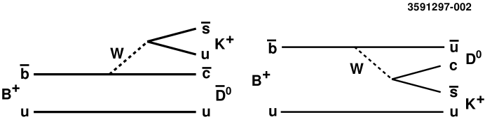
FIG. 1.: Dominant Feynman diagrams of $B^{+}\rightarrow\bar{D}^{0}K^{+}$ and $B^{+}\rightarrow D^{0}K^{+}$.

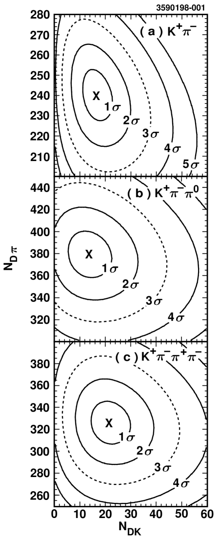
FIG. 2.: Contour plots of $-2\ln{\cal L}$ as a function of $N_{DK}$ and $N_{D\pi}$, the number of $B^{+}\rightarrow\bar{D}^{0}K^{+}$ and $B^{+}\rightarrow\bar{D}^{0}\pi^{+}$ events found in the fit, respectively. The dashed line marks the $3\sigma$ contour. (a) $\bar{D}^{0}\rightarrow K^{+}\pi^{-}$, (b) $\bar{D}^{0}\rightarrow K^{+}\pi^{-}\pi^{0}$, (c) $\bar{D}^{0}\rightarrow K^{+}\pi^{-}\pi^{+}\pi^{-}$. Note that the $N_{D\pi}$ axis has a suppressed zero.

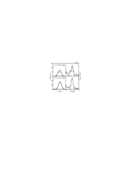
FIG. 3.: Projections onto the $dE/dx$ and $\Delta E$ axes of the data (points) and fit function (solid curves), summed over the three modes. The dashed and dotted curves are the $B^{+}\rightarrow\bar{D}^{0}K^{+}$ and $B^{+}\rightarrow\bar{D}^{0}\pi^{+}$ contributions to the fit functions, respectively. (a) $B^{+}\rightarrow\bar{D}^{0}K^{+}$ region. (b) $B^{+}\rightarrow\bar{D}^{0}\pi^{+}$ region.

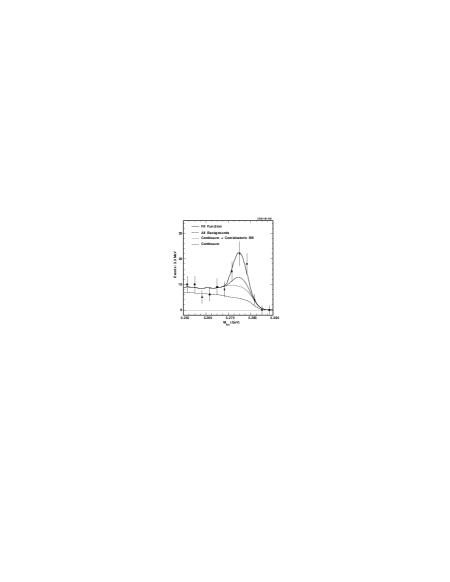
FIG. 4.: Projections onto the $M_{bc}$ axis of the data (points) and fit function (solid curve) in the $B^{+}\rightarrow\bar{D}^{0}K^{+}$ region, summed over the three modes. Also shown are separate background contribtions to the fit function: Continuum, continuum plus combinatoric $B\bar{B}$ events with a misreconstructed $\bar{D}^{0}$, and all backgrounds (including $B^{+}\rightarrow\bar{D}^{0}\pi^{+}$).

REFERENCES

- [1] M. Gronau and D. Wyler, Phys. Lett. B265, 172 (1991); I. Dunietz, Phys. Lett. B270, 75 (1991); D. Atwood, G. Eilam, M. Gronau and A. Soni, Phys. Lett. B341 372 (1995); D. Atwood, I. Dunietz and A. Soni, Phys. Rev. Lett. 78, 3257 (1997).
- [2] M. Kobayashi and K. Maskawa, Prog. Theor. Phys. 49, 652 (1973).
- [3] CLEO Collaboration, Y. Kubota et al., Nucl. Instrum. Methods Phys. Res., Sec. A320, 66 (1992).
- [4] CLEO Collaboration, D. M. Asner et al., Phys. Rev. D 53, 1039 (1996).
- [5] G. Fox and S. Wolfram, Phys. Rev. Lett. 41, 1581 (1978).
- [6] ARGUS Collaboration, H. Albrecht et al., Phys. Lett. B 254, 288 (1991).
- [7] M. Bauer, B. Stech and M. Wirbel, Z. Phys. C34, 103 (1987).
- [8] R. Brun et al., GEANT 3.15, CERN DD/EE/84-1.
- [9] CLEO Collaboration, B. Barish et al., CLEO CONF 97-01, EPS 339.
- [10] R.M. Barnett et al., (Particle Data Group), Phys. Rev. D54, 1 (1996).
- [11] CLEO Collaboration, J. P. Alexander et al., ICHEP-96 PA05-68, CLEO CONF 96-27.