Observation of Exclusive Two-body B Decays to Kaons and Pions

Abstract

We have studied two-body charmless hadronic decays of $B$ mesons into the final states $\pi\pi$, $K\pi$, and $KK$. Using 3.3 million $B\bar{B}$ pairs collected with the CLEO-II detector, we have made the first observation of the decays $B^{0}\to K^{+}\pi^{-}$, $B^{+}\to K^{0}\pi^{+}$, and the sum of $B^{+}\rightarrow\pi^{+}\pi^{0}$ and $B^{+}\rightarrow K^{+}\pi^{0}$ decays (an average over charge-conjugate states is always implied). We place upper limits on branching fractions for the remaining decay modes.

R. Godang,¹ K. Kinoshita,¹ I. C. Lai,¹ P. Pomianowski,¹ S. Schrenk,¹ G. Bonvicini,² D. Cinabro,² R. Greene,² L. P. Perera,² G. J. Zhou,² M. Chadha,³ S. Chan,³ G. Eigen,³ J. S. Miller,³ C. O’Grady,³ M. Schmidtler,³ J. Urheim,³ A. J. Weinstein,³ F. Würthwein,³ D. W. Bliss,⁴ G. Masek,⁴ H. P. Paar,⁴ S. Prell,⁴ V. Sharma,⁴ D. M. Asner,⁵ J. Gronberg,⁵ T. S. Hill,⁵ D. J. Lange,⁵ R. J. Morrison,⁵ H. N. Nelson,⁵ T. K. Nelson,⁵ D. Roberts,⁵ A. Ryd,⁵ R. Balest,⁶ B. H. Behrens,⁶ W. T. Ford,⁶ H. Park,⁶ J. Roy,⁶ J. G. Smith,⁶ J. P. Alexander,⁷ R. Baker,⁷ C. Bebek,⁷ B. E. Berger,⁷ K. Berkelman,⁷ K. Bloom,⁷ V. Boisvert,⁷ D. G. Cassel,⁷ D. S. Crowcroft,⁷ M. Dickson,⁷ S. von Dombrowski,⁷ P. S. Drell,⁷ K. M. Ecklund,⁷ R. Ehrlich,⁷ A. D. Foland,⁷ P. Gaidarev,⁷ R. S. Galik,⁷ L. Gibbons,⁷ B. Gittelman,⁷ S. W. Gray,⁷ D. L. Hartill,⁷ B. K. Heltsley,⁷ P. I. Hopman,⁷ J. Kandaswamy,⁷ P. C. Kim,⁷ D. L. Kreinick,⁷ T. Lee,⁷ Y. Liu,⁷ N. B. Mistry,⁷ C. R. Ng,⁷ E. Nordberg,⁷ M. Ogg,^7, J. R. Patterson,⁷ D. Peterson,⁷ D. Riley,⁷ A. Soffer,⁷ B. Valant-Spaight,⁷ C. Ward,⁷ M. Athanas,⁸ P. Avery,⁸ C. D. Jones,⁸ M. Lohner,⁸ S. Patton,⁸ C. Prescott,⁸ J. Yelton,⁸ J. Zheng,⁸ G. Brandenburg,⁹ R. A. Briere,⁹ A. Ershov,⁹ Y. S. Gao,⁹ D. Y.-J. Kim,⁹ R. Wilson,⁹ H. Yamamoto,⁹ T. E. Browder,¹⁰ Y. Li,¹⁰ J. L. Rodriguez,¹⁰ T. Bergfeld,¹¹ B. I. Eisenstein,¹¹ J. Ernst,¹¹ G. E. Gladding,¹¹ G. D. Gollin,¹¹ R. M. Hans,¹¹ E. Johnson,¹¹ I. Karliner,¹¹ M. A. Marsh,¹¹ M. Palmer,¹¹ M. Selen,¹¹ J. J. Thaler,¹¹ K. W. Edwards,¹² A. Bellerive,¹³ R. Janicek,¹³ D. B. MacFarlane,¹³ P. M. Patel,¹³ A. J. Sadoff,¹⁴ R. Ammar,¹⁵ P. Baringer,¹⁵ A. Bean,¹⁵ D. Besson,¹⁵ D. Coppage,¹⁵ C. Darling,¹⁵ R. Davis,¹⁵ S. Kotov,¹⁵ I. Kravchenko,¹⁵ N. Kwak,¹⁵ L. Zhou,¹⁵ S. Anderson,¹⁶ Y. Kubota,¹⁶ S. J. Lee,¹⁶ J. J. O’Neill,¹⁶ R. Poling,¹⁶ T. Riehle,¹⁶ A. Smith,¹⁶ M. S. Alam,¹⁷ S. B. Athar,¹⁷ Z. Ling,¹⁷ A. H. Mahmood,¹⁷ S. Timm,¹⁷ F. Wappler,¹⁷ A. Anastassov,¹⁸ J. E. Duboscq,¹⁸ D. Fujino,^18, K. K. Gan,¹⁸ T. Hart,¹⁸ K. Honscheid,¹⁸ H. Kagan,¹⁸ R. Kass,¹⁸ J. Lee,¹⁸ M. B. Spencer,¹⁸ M. Sung,¹⁸ A. Undrus,^18, R. Wanke,¹⁸ A. Wolf,¹⁸ M. M. Zoeller,¹⁸ B. Nemati,¹⁹ S. J. Richichi,¹⁹ W. R. Ross,¹⁹ H. Severini,¹⁹ P. Skubic,¹⁹ M. Bishai,²⁰ J. Fast,²⁰ J. W. Hinson,²⁰ N. Menon,²⁰ D. H. Miller,²⁰ E. I. Shibata,²⁰ I. P. J. Shipsey,²⁰ M. Yurko,²⁰ S. Glenn,²¹ S. D. Johnson,²¹ Y. Kwon,^21, S. Roberts,²¹ E. H. Thorndike,²¹ C. P. Jessop,²² K. Lingel,²² H. Marsiske,²² M. L. Perl,²² V. Savinov,²² D. Ugolini,²² R. Wang,²² X. Zhou,²² T. E. Coan,²³ V. Fadeyev,²³ I. Korolkov,²³ Y. Maravin,²³ I. Narsky,²³ V. Shelkov,²³ J. Staeck,²³ R. Stroynowski,²³ I. Volobouev,²³ J. Ye,²³ M. Artuso,²⁴ F. Azfar,²⁴ A. Efimov,²⁴ M. Goldberg,²⁴ D. He,²⁴ S. Kopp,²⁴ G. C. Moneti,²⁴ R. Mountain,²⁴ S. Schuh,²⁴ T. Skwarnicki,²⁴ S. Stone,²⁴ G. Viehhauser,²⁴ X. Xing,²⁴ J. Bartelt,²⁵ S. E. Csorna,²⁵ V. Jain,^25, K. W. McLean,²⁵ and S. Marka²⁵

The phenomenon of $CP$ violation, so far observed only in the neutral kaon system, can be accommodated by a complex phase in the Cabibbo-Kobayashi-Maskawa (CKM) quark-mixing matrix [1]. Whether this phase is the correct, or only, source of $CP$ violation awaits experimental confirmation. $B$ meson decays, in particular charmless $B$ meson decays, will play an important role in verifying this picture.

The decay $B^{0}\rightarrow\pi^{+}\pi^{-}$, dominated by the $b\rightarrow u$ tree diagram (Fig. 1(a)), can be used to measure $CP$ violation due to $B^{0}-\bar{B}^{0}$ mixing at both asymmetric $B$ factories and hadron colliders. However, theoretical uncertainties due to the presence of the $b\to dg$ penguin diagram (Fig. 1(b)) make it difficult to extract the angle $\alpha$ of the unitarity triangle from $B^{0}\rightarrow\pi^{+}\pi^{-}$ alone. Additional measurements of $B^{+}\rightarrow\pi^{+}\pi^{0}$, $B^{0}\rightarrow\pi^{0}\pi^{0}$, and the use of isospin symmetry may resolve these uncertainties [2].

$B\to K\pi$ decays are dominated by the $b\rightarrow sg$ gluonic penguin diagram, with additional contributions from $b\rightarrow u$ tree and color-allowed electroweak penguin (Fig. 1(d)) processes. Interference between the penguin and spectator amplitudes can lead to direct $CP$ violation, which would manifest itself as a rate asymmetry for decays of $B$ and $\bar{B}$ mesons. Recently, the ratio $R={\cal B}(B\to K^{\pm}\pi^{\mp})/{\cal B}(B^{\pm}\to K^{0}\pi^{\pm})$, was shown [3] to constrain $\gamma$, the phase of $V_{ub}$. Several methods of measuring $\gamma$ using only decay rates of $B\to K\pi,~{}\pi\pi$ processes were also proposed [4]. This is particularly important, as $\gamma$ is the least known parameter of the unitarity triangle and is likely to remain the most difficult to determine experimentally. This Letter describes the first measurement of exclusive charmless hadronic $B$ decays. Previous measurements existed only for the sum of several two-body final states [5, 6].

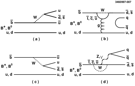
FIG. 1.: The dominant decay processes are expected to be (a) external W-emission, (b) gluonic penguin, (c) internal W-emission, (d) external electroweak penguin.

The data set used in this analysis was collected with the CLEO-II detector [7] at the Cornell Electron Storage Ring (CESR). It consists of $3.14~{}{\rm fb}^{-1}$ taken at the $\Upsilon$(4S) (on-resonance) and $1.62~{}{\rm fb}^{-1}$ taken below $B\bar{B}$ threshold. The on-resonance sample contains 3.3 million $B\bar{B}$ pairs. The below-threshold sample is used for continuum background studies.

Charged tracks are required to pass track quality cuts based on the average hit residual and the impact parameters in both the $r-\phi$ and $r-z$ planes. Pairs of tracks with vertices displaced by at least $3$ mm from the primary interaction point are taken as $K_{S}^{0}$ candidates. We require the $\pi^{+}\pi^{-}$ invariant mass to be within $10$ MeV, two standard deviations ($\sigma$), of the $K^{0}_{S}$ mass. Isolated showers with energies greater than $30$ MeV in the central region of the CsI calorimeter and greater than $50$ MeV elsewhere, are defined to be photons. Pairs of photons with an invariant mass within $20$ MeV ($\sim 2\sigma$) of the nominal $\pi^{0}$ mass are kinematically fitted with the mass constrained to the $\pi^{0}$ mass. To reduce combinatoric backgrounds we require the lateral shapes of the showers to be consistent with those from photons, and that $|\cos\theta^{*}|<0.97$, where $\theta^{*}$ is the angle between the direction of flight of the $\pi^{0}$ and the photons in the $\pi^{0}$ rest frame.

Charged particles are identified as kaons or pions using $dE/dx$. Electrons are rejected based on $dE/dx$ and the ratio of the track momentum to the associated shower energy in the CsI calorimeter. We reject muons by requiring that the tracks do not penetrate the steel absorber to a depth greater than five nuclear interaction lengths. We have studied the $dE/dx$ separation between kaons and pions for momenta $p\sim 2.6$ GeV$/c$ in data using $D^{*+}$-tagged $D^{0}\rightarrow K^{-}\pi^{+}$ decays; we find a separation of $(1.7\pm 0.1)\sigma$.

We calculate a beam-constrained $B$ mass $M=\sqrt{E_{\rm b}^{2}-p_{B}^{2}}$, where $p_{B}$ is the $B$ candidate momentum and $E_{\rm b}$ is the beam energy. The resolution in $M$ ranges from 2.5 to 3.0 ${\rm MeV}/{\it c}^{2}$, where the larger resolution corresponds to decay modes with $\pi^{0}$’s. We define $\Delta E=E_{1}+E_{2}-E_{\rm b}$, where $E_{1}$ and $E_{2}$ are the energies of the daughters of the $B$ meson candidate. The resolution on $\Delta E$ is mode-dependent and ranges from $\pm 26$ MeV for $K^{0}_{S}\pi^{+}$ to $+82/-162$ MeV for $\pi^{0}\pi^{0}$. The latter resolution is asymmetric because of energy loss out of the back of the CsI crystals. The energy constraint also helps to distinguish between modes of the same topology. For example, $\Delta E$ for $B^{0}\rightarrow K^{+}\pi^{-}$, calculated assuming $B^{0}\rightarrow\pi^{+}\pi^{-}$, has a distribution that is centered at $-42$ MeV, giving a separation of $1.6\sigma$ between $B^{0}\rightarrow K^{+}\pi^{-}$ and $B^{0}\rightarrow\pi^{+}\pi^{-}$. We accept events with $M$ within $5.2-5.3$ $\rm{GeV/c^{2}}$ and $|\Delta E|<200(300)$ MeV for decay modes without (with) a $\pi^{0}$ in the final state. This fiducial region includes the signal region, and a sideband for background determination.

We have studied backgrounds from $b\to c$ decays and other $b\to u$ and $b\to s$ decays and find that all are negligible for the analyses presented here. The main background arises from $e^{+}e^{-}\to q\bar{q}$ (where $q=u,d,s,c$). Such events typically exhibit a two-jet structure and can produce high momentum back-to-back tracks in the fiducial region. To reduce contamination from these events, we calculate the angle $\theta_{S}$ between the sphericity axis of the candidate tracks and showers and the sphericity axis of the rest of the event. The distribution of $\cos\theta_{S}$ is strongly peaked at $\pm 1$ for $q\bar{q}$ events and is nearly flat for $B\bar{B}$ events. We require $|\cos\theta_{S}|<0.8$ which eliminates $83\%$ of the background. Using a detailed GEANT-based Monte-Carlo simulation [8] we determine overall detection efficiencies (${\cal E}$) of $5-44\%$, as listed in Table I. Efficiencies contain branching fractions for $K^{0}\to K^{0}_{S}\to\pi^{+}\pi^{-}$ and $\pi^{0}\to\gamma\gamma$ where applicable. We estimate a systematic error on the efficiency using independent data samples.

Additional discrimination between signal and $q\bar{q}$ background is provided by a Fisher discriminant technique as described in detail in Ref. [5]. The Fisher discriminant is a linear combination ${\cal F}\equiv\sum_{i=1}^{N}\alpha_{i}y_{i}$ where the coefficients $\alpha_{i}$ are chosen to maximize the separation between the signal and background Monte-Carlo samples. The 11 inputs, $y_{i}$, are $|\cos\theta_{cand}|$ (the cosine of the angle between the candidate sphericity axis and beam axis), the ratio of Fox-Wolfram moments $H_{2}/H_{0}$ [9], and nine variables that measure the scalar sum of the momenta of tracks and showers from the rest of the event in nine angular bins, each of $10^{\circ}$, centered about the candidate’s sphericity axis.

TABLE I.: Experimental results and theoretical predictions [10]. Branching fractions (${\cal B}$) and 90% C.L. upper limits are given in $10^{-5}$ units. Quoted significance of the fit results is statistical only. The errors on ${\cal B}$ are statistical, fit systematics, and efficiency systematics respectively.

Mode	$N_{S}$	Sig.	${\cal E}(\%)$	${\cal B}$	Theory ${\cal B}$
$\pi^{+}\pi^{-}$	$9.9^{+6.0}_{-5.1}$	2.2$\sigma$	$44\pm 3$	$<~{}1.5$	0.8–2.6
$\pi^{+}\pi^{0}$	$11.3^{+6.3}_{-5.2}$	2.8$\sigma$	$37\pm 3$	$<~{}2.0$	0.4–2.0
$\pi^{0}\pi^{0}$	$2.7^{+2.7}_{-1.7}$	2.4$\sigma$	$29\pm 3$	$<0.93$	0.006–0.1
$K^{+}\pi^{-}$	$21.6^{+6.8}_{-6.0}$	5.6$\sigma$	$44\pm 3$	$1.5^{+0.5}_{-0.4}\pm 0.1\pm 0.1$	0.7–2.4
$K^{+}\pi^{0}$	$8.7^{+5.3}_{-4.2}$	2.7$\sigma$	$37\pm 3$	$<~{}1.6$	0.3–1.3
$K^{0}\pi^{+}$	$9.2^{+4.3}_{-3.8}$	3.2$\sigma$	$12\pm 1$	$2.3^{+1.1}_{-1.0}\pm 0.3\pm 0.2$	0.8–1.5
$K^{0}\pi^{0}$	$4.1^{+3.1}_{-2.4}$	2.2$\sigma$	$8\pm 1$	$<~{}4.1$	0.3–0.8
$K^{+}K^{-}$	$0.0^{+1.3}_{-0.0}$	0.0$\sigma$	$44\pm 3$	$<~{}0.43$	–
$K^{+}\bar{K}^{0}$	$0.6^{+3.8}_{-0.6}$	0.2$\sigma$	$12\pm 1$	$<~{}2.1$	0.07–0.13
$K^{0}\bar{K}^{0}$	0	–	$5\pm 1$	$<~{}1.7$	0.07–0.12
$h^{+}\pi^{0}$	$20.0^{+6.8}_{-5.9}$	5.5$\sigma$	$37\pm 3$	$1.6^{+0.6}_{-0.5}\pm 0.3\pm 0.2$	–

For all modes except $B^{0}\to K^{0}\bar{K}^{0}$ we perform unbinned maximum-likelihood (ML) fits using $\Delta E$, $M$, ${\cal F}$, $|\cos\theta_{B}|$ (the angle between the $B$ meson momentum and beam axis), and $dE/dx$ (where applicable) as input information for each candidate event to determine the signal yields. Five different fits are performed, one for each topology ($h^{+}h^{-}$, $h^{+}\pi^{0}$, $\pi^{0}\pi^{0}$, $h^{+}K^{0}_{S}$, and $K^{0}_{S}\pi^{0}$, $h^{\pm}$ referring to a charged kaon or pion). In each of these fits the likelihood of the event is parameterized by the sum of probabilities for all relevant signal and background hypotheses, with relative weights determined by maximizing likelihood function ($\cal L$). The probability of a particular hypothesis is calculated as a product of the probability density functions (PDF’s) for each of the input variables. The PDF’s of the input variables are parameterized by a Gaussian, a bifurcated Gaussian, or a sum of two bifurcated Gaussians, except for $|\cos\theta_{B}|$ ($1-|\cos\theta_{B}|^{2}$ for signal, constant for background), background $\Delta E$ (straight line), and background $M$ ($f(M)\propto M\sqrt{1-x^{2}}\exp[-\gamma(1-x^{2})]$; $x=M/E_{b}$)  [11].

The parameters for the PDF’s are determined from independent data and high-statistics Monte-Carlo samples. We estimate a systematic error on the fitted yield by varying the PDF’s used in the fit. The error is dominated by the limited statistics in the independent data samples we used to determine the PDF’s. Further details about the likelihood fit can be found in Ref. [5].

Figure 2 shows contour plots of $-2\ln{\cal L}$ for the ML fits to the signal yields ($N$). The curves represent the $n\sigma$ contours ($n=1-5$), which correspond to the increase in $-2\ln{\cal L}$ by $n^{2}$. The dashed curve marks the $3\sigma$ contour. The statistical significance of a given signal yield is determined by repeating the fit with the signal yield fixed to be zero and recording the change in $-2\ln{\cal L}$. To further illustrate the fits, Fig. 3 shows $M$ ($\Delta E$) projections for events in a signal region defined by $|\Delta E|<2\sigma_{\Delta E}$ ( $|M-5.28|<2\sigma_{M}$). We also make a cut on ${\cal F}$ which keeps $67\%$ of the signal and rejects $80\%$ of the background. For Fig. 3(a), events are sorted by $dE/dx$ according to the most likely hypothesis. For Fig. 3(c), $3\sigma$ consistency with the pion hypothesis is required. Overlaid on these plots are the projections of the PDF’s used in the fit, normalized according to the fit results multiplied by the efficiency of the additional cuts ($\sim 60-70\%$ for the signal and $\sim 2-10\%$ for the background). The central values of the signal yields from the fits ($N_{S}$) are given in Table I. We find statistically significant signals for the decays $B^{0}\to K^{+}\pi^{-}$

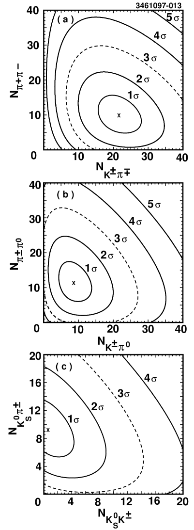
FIG. 2.: Contours of the $-2\ln{\cal L}$ for the ML fits to (a) $N_{K^{\pm}\pi^{\mp}}$ and $N_{\pi^{+}\pi^{-}}$ for $B^{0}\rightarrow K^{+}\pi^{-}$ and $B^{0}\rightarrow\pi^{+}\pi^{-}$; (b) $N_{K\pi^{0}}$ and $N_{\pi\pi^{0}}$ for $B^{+}\rightarrow K^{+}\pi^{0}$ and $B^{+}\rightarrow\pi^{+}\pi^{0}$; (c) $N_{K^{0}_{S}K}$ and $N_{K^{0}_{S}\pi}$ for $B^{+}\rightarrow\bar{K}^{0}K^{+}$ and $B^{+}\rightarrow K^{0}\pi^{+}$.

and $B^{+}\to K^{0}\pi^{+}$. The latter mode constitutes the first unambiguous observation of a gluonic penguin decay. The former mode may have a sizeable contribution from the color-allowed $b\rightarrow u$ tree-level spectator diagram in addition to the dominant gluonic penguin amplitude.

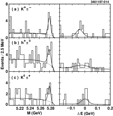
FIG. 3.: $M$ and $\Delta E$ plots for (a) $B^{0}\rightarrow K^{+}\pi^{-}$, (b) $B^{+}\rightarrow h^{+}\pi^{0}$, and (c) $B^{+}\rightarrow K^{0}\pi^{+}$. The scaled projection of the total likelihood fit (solid curve) and the continuum background component (dotted curve) are overlaid.

We also observe a significant signal in the sum of decays $B^{+}\to K^{+}\pi^{0}$ and $B^{+}\to\pi^{+}\pi^{0}$.

As a cross-check, we perform a counting analysis in the modes $B^{0}\rightarrow K^{+}\pi^{-},~{}B^{+}\to K^{0}\pi^{+}$, and $B^{+}\to h^{+}\pi^{0}$. We calculate the probability of the background fluctuation to produce the excess of events shown in Fig. 3 to be $2.0\times 10^{-7}$ for the $K^{+}\pi^{-}$ mode, $1.6\times 10^{-3}$ for the $h^{+}\pi^{0}$ mode, and $2.5\times 10^{-4}$ for the $K^{0}\pi^{+}$ mode.

The statistical significance of the fitted yields in the modes $\pi^{+}\pi^{-},\ \pi^{+}\pi^{0},\ \pi^{0}\pi^{0},\ K^{+}\pi^{0}$, and $K^{0}\pi^{0}$ ranges from $2.2\sigma$ to $2.8\sigma$. We consider these to be not statistically significant and calculate $90\%$ confidence level (C.L.) upper limit yields by integrating the likelihood function

$${\int_{0}^{N^{UL}}{\cal L}_{\rm max}(N)dN\over\int_{0}^{\infty}{\cal L}_{\rm max}(N)dN}=0.90$$ (1)

where ${\cal L}_{\rm max}(N)$ is the maximum $\cal L$ at fixed $N$ to conservatively account for possible correlations among the free parameters in the fit. We then increase upper limit yields by their systematic errors and reduce detection efficiencies by their systematic errors to calculate branching fraction upper limits given in Table I.

We search for the decay $B^{0}\to K^{0}\bar{K}^{0}$ via $K^{0},\bar{K}^{0}\to K^{0}_{S}\to\pi^{+}\pi^{-}$. Since the background for this decay is quite low, the complication of a ML fit is not necessary and a simple counting analysis is used. Event selection is as described above, except no Fisher discriminant is used and $|\cos\theta_{T}|<0.75$ cut is applied ($\cos\theta_{T}$ is defined similar to $\cos\theta_{S}$, but with thrust axis used instead of sphericity). We define the signal region by requiring $|\Delta E|<65$ MeV ($2.5\sigma$), and $|M-5.28|<0.005$ GeV$/c^{2}$ ($2.4\sigma$). We observe no events in the signal region and calculate a $90\%$ C.L. branching fraction upper limit of ${\cal B}(B^{0}\to K^{0}\bar{K^{0}})<1.7\times 10^{-5}$.

As a comparison, we relate $B\to\pi l\nu$ and $B\to\pi\pi$ processes within the factorization hypothesis. Using the ISGW II [12] form factors, the QCD factor $a_{1}=1.03\pm 0.07$ [13], and the CLEO measurement ${\cal B}(B^{0}\to\pi^{-}l^{+}\nu)=(1.8\pm 0.4\pm 0.3\pm 0.2)\times 10^{-4}$ [14], we predict ${\cal B}(B^{0}\to\pi^{+}\pi^{-})=(1.2\pm 0.4)\times 10^{-5}$ and ${\cal B}(B^{+}\to\pi^{+}\pi^{0})=(0.6\pm 0.2)\times 10^{-5}$ [15]. These predictions are consistent with our upper limits as well as central values from the fit: ${\cal B}(B^{0}\to\pi^{+}\pi^{-})=(0.7\pm 0.4)\times 10^{-5}$ and ${\cal B}(B^{+}\to\pi^{+}\pi^{0})=(0.9^{+0.6}_{-0.5})\times 10^{-5}$.

In summary, we have measured branching fractions for two of the four exclusive $B\to K\pi$ decays, while only upper limits could be established for the processes $B\to\pi\pi,KK$. Our results therefore indicate that the $b\to sg$ penguin amplitude dominates charmless hadronic $B$ decays.

We gratefully acknowledge the effort of the CESR staff in providing us with excellent luminosity and running conditions. This work was supported by the National Science Foundation, the U.S. Department of Energy, the Heisenberg Foundation, the Alexander von Humboldt Stiftung, Research Corporation, the Natural Sciences and Engineering Research Council of Canada, and the A.P. Sloan Foundation.

REFERENCES

- [1] M. Kobayashi and K. Maskawa, Prog. Theor. Phys. 49, 652 (1973).
- [2] M. Gronau and D. London, Phys. Rev. Lett. 65, 3381 (1990).
- [3] R. Fleischer and T. Mannel, Univ. of Karlsruhe preprint TTP 97-17, hep-ph/9704423 (unpublished).
- [4] M. Gronau, J. L. Rosner, and D. London, Phys. Rev. Lett. 73, 21 (1994); R. Fleischer, Phys. Lett. B 365, 399 (1996).
- [5] D. M. Asner et al. (CLEO Collaboration), Phys. Rev. D 53, 1039 (1996).
- [6] D. Buskulic et al. (ALEPH Collaboration), Phys. Lett. B 384, 471 (1996); W. Adam et al. (DELPHI Collaboration), Zeit. Phys. C 72, 207 (1996).
- [7] Y. Kubota et al. (CLEO Collaboration), Nucl. Instrum. Methods Phys. Res., Sec. A320, 66 (1992).
- [8] R. Brun et al., GEANT 3.15, CERN DD/EE/84-1.
- [9] G. Fox and S. Wolfram, Phys. Rev. Lett. 41, 1581 (1978).
- [10] N. G. Deshpande and J. Trampetic, Phys. Rev. D 41, 895 (1990); L.-L. Chau et al., Phys. Rev. D 43, 2176 (1991); A. Deandrea et al., Phys. Lett. B 318, 549 (1993); A. Deandrea et al., Phys. Lett. B 320, 170 (1994); G. Kramer and W. F. Palmer, Phys. Rev. D 52, 6411 (1995); D. Ebert, R. N. Faustov, and V. O. Galkin, Phys. Rev. D 56, 312 (1997); D. Du and L. Guo, Zeit. Phys. C 75, 9 (1997).
- [11] H. Albrecht et al. (ARGUS Collaboration), Phys. Lett. B 241, 278 (1990); H. Albrecht et al. (ARGUS Collaboration), Phys. Lett. B 254, 288 (1991).
- [12] N. Isgur and D. Scora, Phys. Rev. D52, 2783 (1995).
- [13] J. Rodriguez, in Proceedings of the Conference on Physics and Violation, Honolulu, 1997.
- [14] J. Alexander et al. (CLEO Collaboration), Phys. Rev. Lett. 77, 5000 (1996).
- [15] The errors quoted do not include theoretical uncertainties due to the factorization hypothesis or form factors.